Disentangling phase transitions and critical points in the proton-neutron interacting boson model by catastrophe theory

Abstract

We introduce the basic concepts of catastrophe theory needed to derive analytically the phase diagram of the proton-neutron interacting boson model (IBM-2). Previous studies [1, 2, 3] were based on numerical solutions. We here explain the whole IBM-2 phase diagram including the precise order of the phase transitions in terms of the cusp catastrophe.

1 Introduction

In the last twenty years quantum phase transitions (QPT’s) (phase transitions that happen at zero temperature as a function of a control parameter) has been a subject of great interest in different areas of quantum many-body systems. In particular, in Nuclear Physics the study of shape phase transitions is a topic of current interest both theoretical and experimentally [4, 5, 6]. Moreover, in Molecular Physics [7, 8], Quantum Optics [9, 10] and Solid State Physics [11] the interest on QPT’s has grown enormously in recent years.

Strictly speaking, QPT’s take place for large systems in the thermodynamic limit as a discontinuity or singularity in some derivative of the ground state energy. However, finite systems like the atomic nuclei could show the precursors of a phase transition when structural changes in the ground state are observed as a function of the neutron or proton numbers (N,Z) [12]. These transitional nuclei are characterized by specific patterns in the low lying spectrum which could be associated with a critical system. Recently, in the context of the Bohr Hamiltonian [13], F. Iachello has introduced the concept of critical point symmetry [14, 15, 16] that can be applied when the quantum system undergoes transitions between two different shape-phases.

A convenient model to study QPT’s in nuclei is the interacting boson model (IBM) [17]. It is a symmetry dictated model whose building blocks are ideal bosons representing nucleon pairs, with angular momentum zero, $s$ bosons, and two, $d$ bosons. In its simplest version, IBM-1, the dynamical algebra of the model is U(6) and the common symmetry algebra O(3). IBM-1 presents three dynamical symmetries (SU(5), O(6), and SU(3)) corresponding to well defined nuclear shapes (spherical, $\gamma$-unstable, and axially deformed, respectively). The presence of different dynamical symmetries in the model is a key ingredient to study QPT’s, since they appear when two different symmetries are mixed in the Hamiltonian through a control parameter: $H(\xi)=\xi\cdot H(\mbox{symmetry}_{1})+(1-\xi)\cdot H(\mbox{symmetry}_{2}).$ For a particular value of the control parameter, $\xi_{c}$, the system undergoes a structural QPT from symmetry 1 to symmetry 2.

The geometry and shape phase transitions of the IBM-1 were studied long ago [18, 19, 20] and also more recently the many facets of QPT’s in IBM have been analyzed [5]. A similar kind of study could be extended to the more realistic version of the IBM that includes the proton-neutron degree of freedom, known as IBM-2 [21]. Most of the studies [1, 2, 3] rely on the numerical diagonalization of the IBM-2 Hamiltonian which is restricted to systems with, as maximum, $10$ proton and $10$ neutron bosons, or in the numerical treatments of semiclassical approximations. These numerical studies, that provided a very accurate description of the phase diagrams, could not state in an unambiguous way the classification of phase transition orders. In this letter we present an analytic study of the IBM-2 phase diagram that is able to determine unambiguously the order of the phase transitions present in the two-fluid IBM-2 model making use of the catastrophe theory (CT) [22, 23, 24]. CT allows to analyze energy surfaces depending on various parameters, i.e., families of potentials, that contain several shape variables, providing information on the nature and numbers of minima (also maxima, if they exist), i.e., stability, depth, etc. This analysis leads to a partition of the parameter space into different regions where the energy surface has different qualitative properties (number and nature of maxima and minima) and, in particular, it serves to study and classify the existing QPT’s. Similar studies were carried out for IBM-1 [25], for IBM including configuration mixing [26, 27], for three-components thermodynamic systems [28, 29], and for elementary chemical reactions [30].

2 IBM-2 Hamiltonian

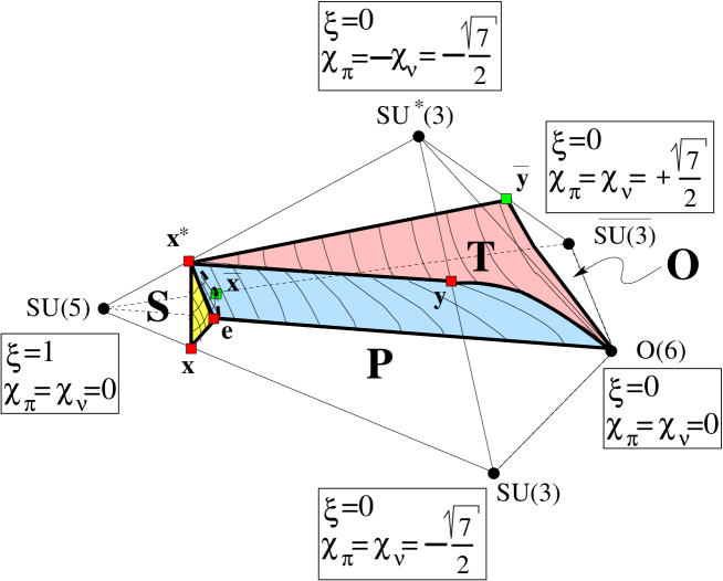
Figure 1: Schematic phase diagram for IBM-2 [1, 2], including the prolate and the oblate sides.

In this work we use a simplified form of the IBM-2 Hamiltonian, known as the Consistent-Q Hamiltonian [31], which retains all the main ingredients of the full Hamiltonian

$$H=\xi\left(n_{d_{\pi}}+n_{d_{\nu}}\right)-\frac{1-\xi}{N}Q^{(\chi_{\pi},\chi_{\nu})}\cdot Q^{(\chi_{\pi},\chi_{\nu})}~{},$$ (1)

where $n_{d_{\rho}}=\sum_{\mu}d_{\rho\mu}^{\dagger}d_{\rho\mu}$, $Q^{(\chi_{\pi},\chi_{\nu})}_{\mu}=\left(Q_{\pi}^{\chi_{\pi}}+Q_{\nu}^{\chi_{\nu}}\right)_{\mu}$ with $Q^{\chi_{\rho}}_{\mu}=\left[d^{\dagger}_{\rho}\widetilde{s}_{\rho}+s^{\dagger}_{\rho}\widetilde{d}_{\rho}\right]_{\mu}^{2}+\chi_{\rho}\left[d^{\dagger}_{\rho}\widetilde{d_{\rho}}\right]_{\mu}^{2}$ and $\rho=\pi,\nu$. $N=N_{\pi}+N_{\nu}$ is the total number of bosons representing the number of valence nucleon pairs.

We study the phase diagram of the IBM-2 in the semi-classical or mean field formalism. In this approach, which is exact in the thermodynamic limit, the ground state wavefunction is a product of a proton condensate times a neutron condensate [32, 33], $|g\rangle=|N_{\pi},N_{\nu},\beta_{\pi},\gamma_{\pi},\beta_{\nu},\gamma_{\nu}\rangle$

$$|g\rangle=\frac{1}{\sqrt{N_{\pi}!N_{\nu}!}}~{}\left(\Gamma^{\dagger}_{\pi}\right)^{N_{\pi}}\left(\Gamma^{\dagger}_{\nu}\right)^{N_{\nu}}|0\rangle~{},$$ (2)

where $|0\rangle$ is the boson vacuum and $\Gamma^{\dagger}_{\rho}$ is the creation operator for a coherent $\pi$ or $\nu$ boson, defined as,

$$\Gamma^{\dagger}_{\rho}=\frac{1}{\sqrt{1+\beta_{\rho}^{2}}}\left[s_{\rho}^{\dagger}+\beta_{\rho}\cos\gamma_{\rho}d^{\dagger}_{\rho 0}+{1\over\sqrt{2}}~{}\beta_{\rho}\sin\gamma_{\rho}(d^{\dagger}_{\rho 2}+d^{\dagger}_{\rho-2})\right]~{}.$$ (3)

The equilibrium values of the structure parameters ($\beta_{\pi},\gamma_{\pi},\beta_{\nu},\gamma_{\nu}$) and the energy of the system for given values of the control parameters ($\xi$, $\chi_{\pi}$, $\chi_{\nu}$) in the Hamiltonian (1) can be obtained by minimizing its expectation value in the intrinsic state (2): $\delta\langle g|H|g\rangle=0$. In the limit $N_{\pi},N_{\nu}\rightarrow\infty$ the energy per boson can be obtained in a straightforward way as

$$E(\beta_{\pi},\gamma_{\pi},\beta_{\nu},\gamma_{\nu};\chi_{\pi},\chi_{\nu},\xi)=\frac{\xi}{2}\sum_{\rho=\pi,\nu}\frac{\beta_{\rho}^{2}}{1+\beta_{\rho}^{2}}-\frac{1-\xi}{4}\sum_{\mu=0,\pm 2}\left[\sum_{\rho=\pi,\nu}\left(Q^{\chi_{\rho}}_{\mu}(\rho)\right)^{2}+2~{}\left(Q^{\chi_{\pi}}_{\mu}(\pi)\right)\left(Q^{\chi_{\nu}}_{-\mu}(\nu)\right)\right]$$ (4)

with

$$Q^{\chi_{\rho}}_{0}(\rho) = \frac{1}{1+\beta_{\rho}^{2}}{\left[2\beta_{\rho}\cos\gamma_{\rho}-\sqrt{\frac{2}{7}}\beta_{\rho}^{2}\chi_{\rho}\cos(2\gamma_{\rho})\right]}$$ (5)

$$Q^{\chi_{\rho}}_{2}(\rho)=Q^{\chi_{\rho}}_{-2}(\rho) = \frac{1}{1+\beta_{\rho}^{2}}\left[\sqrt{2}\beta_{\rho}\sin\gamma_{\rho}+\sqrt{\frac{1}{7}}\beta_{\rho}^{2}\chi_{\rho}\sin(2\gamma_{\rho})\right].$$ (6)

Notice that Hamiltonian (1) can only lead to energy surfaces where proton and neutron ellipsoids are axially symmetric with symmetry axis either parallel or perpendicular, or to triaxial shapes in both ellipsoids (see [34] for details). Therefore, it is not required to include explicitly the Euler angles.

In order to analyze the energy surface it is convenient to introduce new variables,

$$\chi=\frac{\chi_{\pi}+\chi_{\nu}}{2},\qquad\chi^{\prime}=\frac{\chi_{\pi}-\chi_{\nu}}{2}.$$ (7)

In Fig. 1 we depict the phase diagram of the model, which has been obtained numerically [1, 2, 3]. The different phases correspond to the spherical region $S$, the prolate axially deformed region $P$, the oblate axially deformed region $O$, and the region with triaxial shapes $T$. It is interesting to note that the IBM-1 phase diagram is recovered for $\chi^{\prime}=0$. The phase diagram could also be extended to positive values of $\chi^{\prime}$, by reflection in the horizontal plane.

The orders of the different phase transitions were inferred from the numerical calculations in [1, 2, 3]. All references coincide in the following classification:

• the $x-x^{*}-e-x$ surface: (equally the surface $\overline{x}-x^{*}-e-\overline{x}$ in the extended diagram to include oblate shapes) is first order, except for the $x^{*}-e$ line, which was proposed to be second order.

• the $x^{*}-e-O(6)-y-x^{*}$ surface: (equally the surface $x^{*}-e-O(6)-\overline{y}-x^{*}$ in the extended diagram to include oblate shapes) is second order.

• the line $e-x^{*}$: is second order.

• the line $e-O(6)$: is first order.

In what follows we will introduce the basic ingredients of CT to determine in an unambiguous way the properties of the QPTs along the critical lines/surfaces in the IBM-2 phase diagram.

3 Catastrophe theory program

Once the IBM-2 phase diagram is known through a numerical study [1, 2, 3], for the conclusive determination of the order of the phase transitions associated to the obtained critical lines/surfaces it is required an analytic study. CT is specially suited to carry out such analysis.

The basic goal of CT is the study of a potential or, more generically, a family of potentials. As we will see, these potentials comprise three types of points. To begin with, let us assume a system described by a real family of smooth potentials:

$$V(\vec{x},\vec{\lambda})\in\Re$$ (8)

where $\vec{x}\in\Re^{n}$ stand for the state (order) variables and $\vec{\lambda}\in\Re^{r}$ are the control parameters. The majority of points $\vec{x}$ have a nonzero gradient and are called regular points. The points where the gradient vanishes are called stationary or critical points and they can be classified in two groups: i) the points where the determinant of the Hessian matrix is different from zero, called isolated, non-degenerated or Morse points, and ii) the points where the determinant of the Hessian matrix is zero, called non-isolated, degenerated or non-Morse points. In summary, points of a family of smooth potentials can be classified according to their gradient and Hessian matrix ${\cal H}$ as:

• Regular points: $\nabla V\neq 0$.

• Morse points (isolated critical points): $\nabla V=0$ and $|{\cal H}|\neq 0$.

• Non-Morse points (degenerated critical points): $\nabla V=0$ and $|{\cal H}|=0$.

Morse theorem [23, 24] guarantees that around a Morse point, a smooth potential is equivalent to a quadratic form, thanks to a smooth non-linear change of variables. Therefore, the stability of the potential under small perturbation in the parameters is guaranteed in Morse points. At non-Morse points the potential cannot be written as a quadratic form because the Hessian matrix has at least one zero eigenvalue. It is at non-Morse points where CT shows all its power. Let us illustrate the CT program starting with the following expression (see Ref. [24] for a more detailed description),

$$h(\vec{x},\vec{\lambda})=V(\vec{x}+\vec{x}_{0},\vec{\lambda}+\vec{\lambda}_{0})-V(\vec{x}_{0},\vec{\lambda}_{0}),$$ (9)

where $\vec{x}_{0}$ is a degenerated critical point (non-Morse) for the control parameter $\vec{\lambda}_{0}$. We perform a Taylor expansion in the order parameters till k-order. The problem of determinacy consists in getting the Taylor series that can be truncated without loss of substantial information with respect to the original function. The issue of finding the most general family of functions with the smallest dimension, d, which contains the original function, is known as unfolding. The number of parameters appearing in this unfolding is called codimension or number of essential parameters. This number is connected with the number of lowest order terms in the Taylor expansion that can be canceled out. The so called catastrophe germ is obtained when all the unfolding terms go to zero, i.e., all possible terms in the Taylor expansion vanish,

$$g(x)=h(x,0).$$ (10)

The final concept to be introduced is transversality. One says that the original function, $V$ is k transversal when it is isomorphic to the canonical form of the unfolding [23].

Thom’s splitting lemma [22] guarantees that a smooth potential at non-Morse points can be written as the sum of a quadratic form, associated to the subspace with nonzero eigenvalues, plus a function containing the variables associated to the zero eigenvalues of the Hessian matrix. The non-Morse part of the latter is a canonical form called catastrophe function. This function is composed by the catastrophe germ, which only depends on the number of vanishing eigenvalues and on the number of control parameters, and by a universal perturbation that removes the degeneracy and makes the potential structurally stable. The catastrophe germs and the related universal perturbations were listed by Thom for potentials up to two variables and up to five parameters [23, 24]. The transformation into the canonical form only exists for a function which is k transversal. If this is not the case, the function cannot be treated with CT.

The first step in the CT program is to find out the critical points of the energy surface ($\nabla E=0$). Among them, the most important is the most degenerate one. This point is the fundamental root taking place at a definite value of the control parameters which we will call critical values. We next proceed making use of a Taylor expansion of the energy surface around the fundamental root. A Taylor expansion around such a point is also valid for the critical points that arise from the fundamental root when the degeneracy is broken. Depending on the degeneracy of the fundamental root the number of extremes that can be analyzed simultaneously will change.

It is important to note here that if the original function is k determined, then the k-order Taylor expansion can be transformed, under the appropriate non-linear change of variables, into a finite polynomial that is valid in the neighborhood of the critical point and critical control parameter,

$$x^{\prime}_{i}=A_{i}+\delta_{ij}x_{j}+A_{i,jk}x_{j}x_{k}+A_{i,jkl}x_{j}x_{k}x_{l}+\ldots,$$ (11)

where $x_{i}$ stand for the original and $x^{\prime}_{i}$ for the transformed variables. Finally, this polynomial can be written in a canonical form composed by the catastrophe germ plus a generic perturbation. Once the properties of the catastrophe function have been established, the stability of the potential is completely determined. In CT the set of non-Morse points is known as bifurcation set while the ensemble of critical points with equal energy are known as the Maxwell set. If the energy surface is in the neighborhood of a Maxwell set, it possesses a first order phase transition. Conversely, if the potential is close to a bifurcation set, it has a second order phase transition.

When the potential depends on several variables it is important to find out which are the variables involved in the phase transition, since they play the role of order parameters. These variables are associated to the subspace with vanishing Hessian eigenvalues, called bad or essential variables, while there is another set of variables related to the non-vanishing Hessian eigenvalues, called good or non-essential variables. The potential could be separated into a part depending on the essential variables and into another part depending on the non-essential ones by rewriting it in terms of the eigenvectors of the Hessian matrix. As a consequence of the splitting lemma the potential is separated into a function of the essential variables and a sum of quadratic terms associated to the non-essential variables [24]. Therefore, the appearance of critical phenomena is associated exclusively with the behavior of the essential variables.

In next section this program is applied to the two-fluid nuclear IBM-2. It will be shown that the relevant elementary catastrophe for this model is the cusp catastrophe ($A_{+3}$) which is characterized by one state variable ($z$) and two-control parameters ($a,b$). The germ of this catastrophe is $z^{4}$ and the perturbation $az+bz^{2}$.

4 Application of the catastrophe theory program to IBM-2

Even for the restricted Hamiltonian (1) it is not possible to carry out a general analysis of the whole phase diagram due to the large number of shape variables (four in the case of the IBM-2). Moreover, it is a nontrivial task the identification of the appropriate order parameters. In order to proceed with the analysis we will concentrate in the critical surfaces depicted in Fig. 1, which were already studied numerically in [1, 2, 3].

4.1 Spherical-axially deformed energy surface

This surface is marked with points $x-e-\overline{x}-x^{*}-x$ in Fig. 1. It corresponds to a situation in which $\gamma_{\pi,\nu}$ can be assumed to be zero, because in the spherical phase the energy does not depend on $\gamma$, and in the axially deformed phase $\gamma=0$ (or $\gamma=\pi/3$ in the oblate side). This assumption is not valid in the case of the line $e-x^{*}$ as it will be explained later on.

Following the procedure described above, we use the fundamental root corresponding to $\beta_{\pi}=\beta_{\nu}=0$ and $\gamma_{\pi}=\gamma_{\nu}=0$ for $\chi<0$ ($\gamma_{\pi}=\gamma_{\nu}=\pi/3$ for $\chi>0$), to construct the Hessian matrix associated to Eq. (4)

$$\cal{H}=\left(\begin{array}[]{cc}\partial^{2}E/\partial\beta_{\pi}^{2}&\partial^{2}E/\partial\beta_{\pi}\partial\beta_{\nu}\\ \partial^{2}E/\partial\beta_{\nu}\partial\beta_{\pi}&\partial^{2}E/\partial\beta_{\nu}^{2}\end{array}\right)=\left(\begin{array}[]{cc}3\xi-2&2\xi-2\\ 2\xi-2&3\xi-2\end{array}\right).$$ (12)

The two eigenvalues are $5\xi-4$ and $\xi$, and the corresponding eigenvectors eigenvectors are,

$$\beta_{1} = \frac{1}{2}~{}(\beta_{\pi}+\beta_{\nu}),$$ (13)

$$\beta_{2} = \frac{1}{2}~{}(-\beta_{\pi}+\beta_{\nu}).$$ (14)

The eigenvalue associated to $\beta_{1}$ vanishes for $\xi=4/5$ while the one associated to $\beta_{2}$ only vanishes for the trivial case $\xi=0$. Therefore the essential variable turns out to be $\beta_{1}$, while $\beta_{2}$ becomes the non-essential one. If we make an expansion of the energy in terms of $\beta_{1}$ and $\beta_{2}$ we get:

$$E = (5\xi-4)\beta_{1}^{2}+\frac{4\sqrt{2}(1-\xi)\chi}{\sqrt{7}}\beta_{1}^{3}+\Big{(}8-9\xi-\frac{2}{7}(1-\xi)\chi^{2}\Big{)}\beta_{1}^{4}$$ (15)

$$+ \Theta(\beta_{1}^{5})+\xi~{}\beta_{2}^{2}+\Theta(\beta_{1}\beta_{2}^{2},\beta_{2}\beta_{1}^{2}),$$

where the terms $\Theta(\beta_{1}^{5})$ and $\Theta(\beta_{1}\beta_{2}^{2},\beta_{2}\beta_{1}^{2})$ can be canceled through a nonlinear transformation (11) in the non-essential variable. Notice that the expansion (15) has no quadratic term proportional to $\beta_{1}\beta_{2}$ since $\beta_{1}$ and $\beta_{2}$ are eigenvectors of the Hessian matrix. Therefore, $E$ simplifies to

$$E=(5\xi-4){\beta_{1}}^{2}+\frac{4\sqrt{2}(1-\xi)\chi}{\sqrt{7}}{\beta_{1}}^{3}+\Big{(}8-9\xi-\frac{2}{7}(1-\xi)~{}\chi^{2}\Big{)}{\beta_{1}}^{4}+\xi~{}\beta_{2}^{2}.$$ (16)

In order to keep the notation simple we keep the variable $\beta_{2}$, although there, it corresponds to the transformed variable (see Eq. (11)). The most salient feature of equation (16) is the existence of a cubic term, which guarantees that the phase transition around $\xi=4/5$ will always be of first order if $\chi=\frac{\chi_{\pi}+\chi_{\nu}}{2}\neq 0$ [24]. Eq. (16) can be transformed into the cusp catastrophe for which a first order phase transition exists if the linear term is different from zero, which is indeed the case for $\chi\neq 0$.

Following Ref. [25], the critical value of the control parameter $\xi_{c}$ is the solution of the equation:

$$r_{1}=-\frac{1}{2}-\frac{1}{2}\sqrt{1+\frac{r_{2}^{2}}{2}},$$ (17)

where

$$r_{1}=\frac{35\xi_{c}-28}{28+4\chi^{2}(\xi_{c}-1)-21\xi_{c}}$$ (18)

and

$$r_{2}=\frac{8\sqrt{14}\chi(\xi_{c}-1)}{28+4\chi^{2}(\xi_{c}-1)-21\xi_{c}}.$$ (19)

Which leads to the solution:

$$\xi_{c}=\frac{28+2\chi^{2}}{35+2\chi^{2}}.$$ (20)

This expression gives the well known values $\xi_{c}=4/5$ for $\chi=0$ and $\xi_{c}=9/11$ for $\chi=\pm\sqrt{7}/2$, which are also valid for IBM-1. It is important to note that  (20) is independent on $\chi^{\prime}$ which implies that the first order IBM-1 critical line propagates vertically generating a first order critical surface separating spherical and axially deformed shapes in IBM-2, as was already established in [3] using different arguments.

4.2 The $e-x^{*}$ line

This line is a limiting case of the previous energy surface, defined by $\chi=0$ ($\chi_{\pi}=-\chi_{\nu}$). The line has some important differences, which deserve a particular analysis. Along this line $\beta_{\pi}=\beta_{\nu}=\beta$. Moreover, $\gamma_{\pi}=\pi/3-\gamma_{\nu}=\gamma$ cannot be zero because one of the phases is triaxial while the other is $\gamma$ independent. These conditions define the fundamental root be $\beta_{\pi}=\beta_{\nu}=\beta=0$, $\gamma_{\pi}=\gamma_{\nu}=\gamma=\pi/6$.

The Hessian matrix evaluated at the fundamental root can be written as,

$$\cal{H}=\left(\begin{array}[]{cc}\partial^{2}E/\partial\beta^{2}&\partial^{2}E/\partial\beta\partial\gamma\\ \partial^{2}E/\partial\gamma\partial\beta&\partial^{2}E/\partial\gamma^{2}\end{array}\right)=\left(\begin{array}[]{cc}5\xi-4&0\\ 0&0\end{array}\right).$$ (21)

The eigenvalue associated to the variable $\beta$ is $5\xi-4$ and it is canceled for $\xi=4/5$. All derivatives in $\gamma$ at the fundamental root vanish. Thus $\beta$ will be the essential variable and $\gamma$ the non-essential one.

The expansion around the fundamental root gives

$$E=(5\xi-4)\beta^{2}+(8-9\xi)\beta^{4}+\Theta(\beta^{6}),$$ (22)

where the odd powers vanish. Since Eq. (22) does not depend on $\chi$ and it has no cubic term, the whole line $e-x^{*}$ will be second order [24].

4.3 Axially deformed-triaxial surface

This surface is delimited by the points $e-O(6)-y-x^{*}-e$ ($e-O(6)-\overline{y}-\overline{x}^{*}-e$ in the oblate side) in Fig. 1. It represents the most complex situation because the four shape variables ($\beta_{\pi}$, $\gamma_{\pi}$, $\beta_{\nu}$, $\gamma_{\nu}$) have to be treated simultaneously. With the exception for the $y$ point, the $y-O(6)$ line, and the $e-O(6)$ line, which will be treated separately, no simplification is possible.

The fundamental root corresponds to $\gamma_{\pi}=\gamma_{\nu}=0$ ($\gamma_{\pi}=\gamma_{\nu}=\pi/3$ for $\chi>0$). The critical values of $\beta_{\pi}$ and $\beta_{\nu}$ depend on the value of the Hamiltonian parameters, therefore we will proceed to study the Hessian matrix for $\gamma_{\pi}=\gamma_{\nu}=0$. The main feature of this matrix is that

$$\frac{\partial^{2}E}{\partial\beta_{\rho}\partial\gamma_{\rho^{\prime}}}=0,$$ (23)

for $\gamma_{\pi}=\gamma_{\nu}=0$ ($\gamma_{\pi}=\gamma_{\nu}=\pi/3$ for $\chi>0$) where $\rho$ and $\rho^{\prime}$ stand for $\pi,\nu$. This equation implies that $\beta$’s are decoupled from the angular variables. As shown in Ref. [1] the behavior of $\beta$ variables when crossing the axially deformed-triaxial surface is smooth and they are related to the non vanishing eigenvalues of the Hessian matrix. Therefore, the $\beta$’s are non-essential variables. According to the splitting lemma the energy surface can be expanded as a quadratic form in $\beta$’s (except in the line $e-x^{*}$ already discussed) plus an expansion in the $\gamma$ variables. Note that the coefficients will depend on the equilibrium values of $\beta_{\pi}$ and $\beta_{\nu}$, i.e., $\beta_{\pi}^{0}$ and $\beta_{\nu}^{0}$,

$$E = f_{00}(\beta_{\pi}^{0},\beta_{\nu}^{0},\xi,\chi,\chi^{\prime})+f_{11}(\beta_{\pi}^{0},\beta_{\nu}^{0},\xi,\chi,\chi^{\prime})\gamma_{\pi}\gamma_{\nu}+f_{02}(\beta_{\pi}^{0},\beta_{\nu}^{0},\xi,\chi,\chi^{\prime})\gamma_{\nu}^{2}+f_{20}(\beta_{\pi}^{0},\beta_{\nu}^{0},\xi,\chi,\chi^{\prime})\gamma_{\pi}^{2}$$ (24)

$$+ f_{04}(\beta_{\pi}^{0},\beta_{\nu}^{0},\xi,\chi,\chi^{\prime})\gamma_{\nu}^{4}+f_{13}(\beta_{\pi}^{0},\beta_{\nu}^{0},\xi,\chi,\chi^{\prime})\gamma_{\pi}\gamma_{\nu}^{3}+f_{22}(\beta_{\pi}^{0},\beta_{\nu}^{0},\xi,\chi,\chi^{\prime})\gamma_{\pi}^{2}\gamma_{\nu}^{2}$$

$$+ f_{31}(\beta_{\pi}^{0},\beta_{\nu}^{0},\xi,\chi,\chi^{\prime})\gamma_{\pi}^{3}\gamma_{\nu}^{1}+f_{40}(\beta_{\pi}^{0},\beta_{\nu}^{0},\xi,\chi_{\pi},\chi_{\nu})\gamma_{\pi}^{4}+g_{20}(\beta_{\pi}^{0},\beta_{\nu}^{0},\xi,\chi,\chi^{\prime})(\beta_{\pi}-\beta_{\pi}^{0})^{2}$$

$$+ g_{02}(\beta_{\pi}^{0},\beta_{\nu}^{0},\xi,\chi,\chi^{\prime})(\beta_{\nu}-\beta_{\nu}^{0})^{2}+g_{11}(\beta_{\pi}^{0},\beta_{\nu}^{0},\xi,\chi,\chi^{\prime})(\beta_{\pi}-\beta_{\pi}^{0})(\beta_{\nu}-\beta_{\nu}^{0})+\Theta(\gamma^{5})+\Theta(\beta^{3}).$$

$\Theta(\gamma^{5})$ and $\Theta(\beta^{3})$ contain terms with powers in $\gamma$ and $\beta$ equal or higher than $5$ and $3$, respectively. The $f_{ij}$ matrix contains the coefficients multiplying the $\gamma$’s variables, while the $g_{ij}$ matrix those multiplying the $\beta$’s variables.

If we make the expansion in terms of the eigenvalues of the Hessian matrix, $\gamma_{1},\gamma_{2}$ ($\beta_{1},\beta_{2}$), the term $\gamma_{1}\gamma_{2}$ ($\beta_{1}\beta_{2}$) in Eq. (24) will vanish. In what follows we assume that $\gamma_{1}$ has a vanishing eigenvalue while $\gamma_{2}$ has a non-vanishing one. In the case of $\beta$ both eigenvalues are different from zero. Next we perform a nonlinear transformation (11) in $\gamma_{2}$, $\beta_{1}$ and $\beta_{2}$ in order to annihilate every cross term and higher order terms. Due to the structure of (24), after the transformation (11) the energy surface will result in

$$E = {f}_{00}(\beta_{\pi}^{0},\beta_{\nu}^{0},\xi,\chi,\chi^{\prime})+\tilde{f}_{20}(\beta_{\pi}^{0},\beta_{\nu}^{0},\xi,\chi,\chi^{\prime})\gamma_{1}^{2}+\tilde{f}_{40}(\beta_{\pi}^{0},\beta_{\nu}^{0},\xi,\chi,\chi^{\prime})\gamma_{1}^{4}$$ (25)

$$+ \tilde{f}_{02}(\beta_{\pi}^{0},\beta_{\nu}^{0},\xi,\chi,\chi)\gamma_{2}^{2}+\tilde{g}_{20}(\beta_{\pi}^{0},\beta_{\nu}^{0},\xi,\chi,\chi^{\prime})(\beta_{1}-\beta_{1}^{0})^{2}$$

$$+ \tilde{g}_{02}(\beta_{\pi}^{0},\beta_{\nu}^{0},\xi,\chi,\chi^{\prime})(\beta_{2}-\beta_{2}^{0})^{2},$$

where that $\gamma_{2}$, $\beta_{1}$, and $\beta_{2}$ stand for the transformed variables (see Eq. 11). The coefficients $\tilde{f}_{20}$ and $\tilde{f}_{02}$ are the eivenvalues of the matrix $((f_{20},f_{11}),(f_{11},f_{02}))$, while $\tilde{g}_{20}$ and $\tilde{g}_{02}$ are the eivenvalues of $((g_{20},g_{11}),(g_{11},g_{02}))$. The absence of cubic term in the later equation, identifies this critical surface as second order [24]. Eq. (25) is equivalent to the cusp catastrophe without linear term which leads to the existence of a unique second order phase transitions.

4.4 The $e-O(6)$ line

This line is a limiting case of the axially deformed-triaxial surface analyzed in the preceding subsection. However, due to the constraints that can be applied to the order parameters it deserves to be discussed separately. The energy can be written in terms of a Taylor expansion in $\beta$ for two reasons. On the one hand, we will stay in the plane with $\chi_{\pi}=\chi_{\nu}=\chi$, i.e., $\chi^{\prime}=0$. This leads to $\beta_{\pi}=\beta_{\nu}=\beta$ and $\gamma_{\pi}=\gamma_{\nu}=\gamma$. On the other hand, because either $\gamma=0$ (for $\chi<0$) or $\gamma=\pi/3$ (for $\chi>0$), its influence can be absorbed in the $\beta$ variable, in such a way that $\beta>0$ corresponds to $\gamma=0$ while $\beta<0$ to $\gamma=\pi/3$. Therefore, the expression for the energy reduces to

$$E=(5\xi-4)\beta^{2}+\frac{4\sqrt{2}(1-\xi)\chi}{\sqrt{7}}\beta^{3}+\Big{(}8-9\xi-\frac{2}{7}(1-\xi)\chi^{2}\Big{)}\beta^{4}+\Theta(\beta^{5}),$$

where $\Theta(\beta^{5})$ can be canceled through a nonlinear transformation in $\beta$ (11). In this case we are interested in $5\xi-4<0$ while $\chi$ vanishes. In this situation $\beta=0$ is a maximum while $\beta=\pm\sqrt{\frac{4-5\xi}{16-18\xi}}$ are two degenerated minima (note that $\beta$ corresponds to the transformed variable (see Eq. (11)). Therefore the $e-O(6)$ line will be first order as was already established in [35].

5 Summary and conclusions

In this work we introduce the key ingredients of catastrophe theory and we describe the basic program to analyze the stability and to classify the order of the phase transitions that can be developed in a given potential energy. We have applied the program to the case of the IBM-2 using a restricted Hamiltonian which is of great interest in Nuclear Physics. Following this procedure we have been able to determine analytically the order of the phase transitions. Our analytic results confirm previous numerical studies. In particular, we establish in an unambiguous way that the surface $x-e-\overline{x}-x^{*}-x$ (spherical-axially deformed surface) is first order except for the line $e-x^{*}$, which is second order. The surfaces $e-O(6)-y-x^{*}-e$ and $e-O(6)-\overline{y}-x^{*}-e$ (axially deformed-triaxial surfaces) are second order, except for the line $e-O(6)$ which is first order. The relevant catastrophe for the IBM-2 phase diagram is the cusp catastrophe.

The IBM-2 example that we have treated shows that the use of catastrophe theory combined with numerical calculations is able to determine unambiguously the different critical potential energy surfaces present in a phase diagram as well as the order of the phase transitions.

6 Acknowledgments

We thank fruitful discussions with J. Margalef-Roig and S. Miret-Artés. This work was partially supported by the Spanish Ministerio de Economía y Competitividad and the European regional development fund (FEDER) under Project Nos. FIS2011-28738-C02-01, FIS2011-28738-C02-02, FIS2012-34479, and by Junta de Andalucía under Project Nos. FQM160, P11-FQM-7632 and FQM318, as well as by Spanish Consolider-Ingenio 2010 (CPANCSD2007-00042).

References

- [1] J.M. Arias, J.E. García-Ramos, and J. Dukelsky, Phys. Rev. Lett. 93, 212501 (2004).
- [2] M.A. Caprio, F. Iachello, Phys. Rev. Lett. 93, 242502 (2004).
- [3] M.A. Caprio, F. Iachello, Ann. Phys. (N.Y.) 318, 454 (2005).
- [4] R.F. Casten and E.A. McCutchan, J. Phys. G 34, R285 (2007).
- [5] P. Cejnar and J. Jolie, Prog. Part. Nucl. Phys. 62, 210 (2009).
- [6] P. Cejnar, J. Jolie, and R.F. Casten, Rev. Mod. Phys. 82, 2155 (2010).
- [7] F. Iachello and F. Pérez-Bernal, Mol. Phys. 106, 223 (2008).
- [8] P. Pérez-Fernández, J.M. Arias, J.E. García-Ramos, and F. Pérez-Bernal, Phys. Rev. C 83, 062125 (2011).
- [9] C. Emary and T. Brandes, Phys. Rev. Lett. 90, 044101 (2003); Phys. Rev. E 67, 066203 (2003); N. Lambert, C. Emary, and T. Brandes, Phys. Rev. Lett. 92, 073602 (2004).
- [10] L. Amico, R. Fazio, A. Osterloh, and V. Vedral, Rev. Mod. Phys. 80, 517 (2008).
- [11] S. Sachdev, Quantum Phase Transitions (Cambridge University Press, Cambridge, UK, 2011)
- [12] F. Iachello, and N.V. Zamfir, Phys. Rev. Lett. 92, 212501 (2004).
- [13] A. Bohr and B. Mottelson, Nuclear Structure, vol II (Benjamin, Reading, Mass. 1975).
- [14] F. Iachello, Phys. Rev. Lett. 85, 3580 (2000).
- [15] F. Iachello, Phys. Rev. Lett. 87, 052502 (2001).
- [16] F. Iachello, Phys. Rev. Lett. 91, 132502 (2003).
- [17] F. Iachello and A. Arima The Interacting Boson Model (Cambridge University Press, Cambridge, UK, 1987)
- [18] A.E.L. Dieperink, O. Scholten, and F. Iachello, Phys. Rev. Lett. 44, 1747 (1980).
- [19] D.H. Feng, R. Gilmore, and S.R. Deans, Phys. Rev. C 23, 1254 (1981).
- [20] A. Frank, Phys. Rev. C 39, 652 (1989).
- [21] A. Arima, T. Otsuka, F. Iachello, and I. Talmi, Phys. Lett. B 66, 205 (1977).
- [22] R. Thom, Structural stability and morphogenesis (Benjamin, Reading, 1975).
- [23] T. Poston and I.N. Stewart, Catastrophe theory and its applications (Pitman, London, 1978).
- [24] R. Gilmore, Catastrophe theory for scientists and engineers (Wiley, New York, 1981).
- [25] E. López-Moreno and O. Castaños, Phys. Rev. C 54, 2374 (1996).
- [26] V. Hellemans, P. Van Isacker, K. Heyde, ad S. De Baerdemacker, Nucl. Phys. A 789, 164 (2007).
- [27] V. Hellemans, P. Van Isacker, K. Heyde, ad S. De Baerdemacker, Nucl. Phys. A 819, 11 (2009).
- [28] J. Gaite, J. Margalef-Roig, and S. Miret-Artés, Phys. Rev. B 57, 13527 (1998).
- [29] J. Gaite, J. Margalef-Roig, and S. Miret-Artés, Phys. Rev. B 59, 8593 (1999).
- [30] J. Margalef-Roig, S. Miret-Artés, A. Toro-Labbe, J. Phys. Chem. A 104, 11589 (2000).
- [31] R.F. Casten and D.D. Warner, Rev. Mod. Phys. 60, 389 (1988).
- [32] J.N. Ginocchio and M.W. Kirson, Nucl. Phys. A350, 31 (1980).
- [33] J. Dukelsky, G.G. Dussel, and H.M. Sofia, Nucl. Phys. A373, 267 (1980).
- [34] J. N. Ginocchio and A. Leviatan, Ann. Phys. (N.Y.) 216, 152 (1992).
- [35] J. Jolie, R.F. Casten, P. von Brentano, and V. Werner, Ohys. Rev. Lett. 87, 162501 (2001).