Electrical transport through a quantum dot side-coupled to a topological superconductor

Abstract

We propose to measure the differential conductance $G$ as a function of the bias $V$ for a quantum dot side-coupled to a topological superconductor to detect the existence of the chiral Majorana edge states. It turns out that $G$ for the spinless dot is an oscillatory (but not periodic) function of $eV$ due to the coupling to the chiral Majorana edge states, where $-e$ is the charge carried by the electron. The behavior of $G$ versus $eV$ is distinguished from the one for a multi-level dot in three respects. First of all, due to the coupling to the topological superconductor, the value of $G$ will shift upon adding or removing a vortex in the topological superconductor. Next, for an off-resonance dot, the conductance peak in the present case takes a universal value $e^{2}/(2h)$ when the two leads are symmetrically coupled to the dot. Finally, for a symmetric setup and an on-resonance dot, the conductance peak will approach the same universal value $e^{2}/(2h)$ at large bias.

I Introduction

Recently, to search for the topological phases and to study their properties become crucial issues in condensed matter physics. Among these topological matters, Majorana fermions, which were theoretically predicted to exist at the edge or the core of a vortex in a $p_{x}+ip_{y}$-wave superconductor and superfluid,Read-Green ; Gurarie ; MStone attract a lot of attentions. This is largely triggered by the fact that Majorana fermions are stable against local perturbationskitaev2 and obey the non-Abelian statistics,Ivanov so that they have great potential in the applications of fault-tolerant quantum computations.Kitave ; Nayak

Up to now, there are two main theoretical proposals to realize Majorana fermions. One way is to generate a localized Majorana mode at the end of a spin-orbit coupled nanowire subjected to a magnetic field and proximate to an $s$-wave superconductor,Lutchyn-Sau-DasSarma ; Oreg-Refael-Open which is motivated by a model proposed by Kitaev.kitaev2 Experimental evidence for such a Majorana edge mode was obtained in indium antimonide quantum wires.Mourik ; nano Majorana fermions can also be supported in the vortices of $s$-wave superconductors deposited on the surface of a three-dimensional topological insulator.Fu-Kane In particular, chiral Majorana edge states can be created at the interface between a superconductor and the area gapped by ferromagnetic materials.Fu-Kane

One of the challenges in the physics of Majorana fermions is to detect and to verify the existence of Majorana fermions. Several methods have been proposed, including the noise measurement,BD ; NAB resonant Andreev reflection,KTLaw and the $4\pi$-periodic Josephson effect.Lutchyn-Sau-DasSarma ; Oreg-Refael-Open ; Fu-Kane2 ; Law ; IF Recently, several groups proposed to measure the electric transport through a quantum dot (QD) coupled to the end of a one-dimensional ($1$D) topological superconductor (TSC) to detect the existence of Majorana modesLF ; LB ; Vernek as well as their dynamics.Cao Especially, in the case of a spinless QD side-coupled to the end of a TSC, the zero-bias conductance at zero temperature takes the value $e^{2}/(2h)$,LB ; Vernek instead of $e^{2}/h$. This fact has been identified as the evidence of the existence of Majorana end modes. In the present work, we propose to employ the similar idea to detect the chiral Majorana edge states in the TSC.

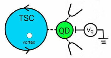
Figure 1: (Color online) A schematic setup of a QD side-coupled to a TSC and to two metallic leads. The dot level can be controlled by a capacitively coupled gate voltage $V_{g}$. The bias is applied between two leads. The TSC is formed by depositing a superconducting island on a three-dimensional topological insulator. The area outside the superconductor is gapped by ferromagnetic materials. At the interface between the superconductor and the ferromagnetic material, there is a branch of chiral Majorana fermions denoted by the arrow.

A schematic setup is shown in Fig. 1. The QD, which can be formed by using either graphenegrap or the carbon nanotube,cnt is side-coupled to a TSC and to two metallic leads. The dot level can be controlled by a capacitively coupled gate voltage $V_{g}$. The bias $V$ is applied between two leads. The TSC is formed by depositing a superconducting island on a three-dimensional ($3$D) topological insulator. (The possible candidates of $3$D topological insulators are Bi₂Se₃ or Bi₂Te₃.3DTI ) The area outside the superconductor is gapped by ferromagnetic materials. At the interface between the superconductor and the ferromagnetic material, there is a branch of chiral Majorana fermions. The presence of the ferromagnetic material removes spin degeneracy of the dot levels. Suppose that the Zeeman splitting is large enough. We may assume that the dot electrons are spinless.foot1 For such a case, we found that the differential conductance $G$ through the spinless dot is an oscillatory (but not periodic) function of $eV$ due to the coupling to the chiral Majorana edge states, where $-e$ is the charge carried by the electron. The behavior of $G$ versus $eV$ in the present case is distinguished from the one for a multi-level dot in three respects. First of all, the value of $G$ for the former will shift upon adding or removing a vortex in the TSC. Next, for an off-resonance dot, the conductance peak for the former takes a universal value $e^{2}/(2h)$ when the two leads are symmetrically coupled to the dot. Finally, for a symmetric setup and an on-resonance dot, the conductance peak in the present case will approach the same universal value $e^{2}/(2h)$ at large bias.

The rest of the paper is organized as follows. We first write down the Hamiltonian which models the setup in Fig. 1 and discuss the approximations we made in the calculations. Next, we present the relevant Green functions to calculate the current through the dot. Then, we give the spectral function of the dot electrons, the differential conductance, and the relevant stuffs. The final section is devoted to a summary of our results.

II The Model

We consider a setup shown in Fig. 1. The TSC is realized by depositing a superconducting island on the surface of a three-dimensional topological insulator. The region outside the superconductor is gapped by ferromagnetic materials. This system can be modeled by the Hamiltonian: $H=H_{C}+H_{D}+H_{T}$, where

$$H_{C}=\!\sum_{\alpha\in L,R}\!\sum_{\bm{k}}\epsilon_{\bm{k}\alpha}c^{\dagger}_{\bm{k}\alpha}c_{\bm{k}\alpha}\ ,$$ (1)

describes the leads, and

$$H_{T}=\!\sum_{\alpha\in L,R}\!\sum_{\bm{k}}\frac{V_{\bm{k}\alpha}}{\sqrt{\Omega}}c^{\dagger}_{\bm{k}\alpha}d+\mathrm{H.c.}\ ,$$ (2)

describes the tunneling between the leads and the dot. The presence of the ferromagnetic material will split the electronic levels of the dot with different spins. We shall focus on the case with large Zeeman splitting such that within the energy scale in which we are interested the dot electrons can be regarded as spinless fermions. We further assume that $eV$ and $k_{B}T$ are much smaller than the superconducting gap in the TSC and the average level spacing in the dot, where $T$ is the temperature. Within these approximations, the Hamiltonian $H_{D}$ can be written as

$$H_{D}=\epsilon_{d}d^{\dagger}d+\frac{v_{M}}{2}\!\!\int^{L/2}_{-L/2}\!dx\eta(-i\partial_{x}\eta)-i\bar{t}\eta(0)(\xi d+\mathrm{H.c.})\ ,$$ (3)

where $\bar{t}>0$ denotes the tunneling amplitude between the dot and the Majorana edge states, $\xi$ is a complex number with $|\xi|=1$, $|v_{M}|$ is the speed of Majorana fermions, and $L$ is the circumference of the island. In Eq. (3), we have taken $x=0$ as the contact point between the TSC and the dot. The dot level $\epsilon_{d}$ can be adjusted by a capacitively coupled gate voltage $V_{g}$.

The real field $\eta(x)$, which describes the chiral Majorana edge states, obeys the anticommutation relation

$$\{\eta(x),\eta(y)\}=\delta(x-y)\ .$$

The Fourier decomposition of $\eta(x)$ is given by

$$\eta(x)=\frac{1}{\sqrt{L}}\sum_{k}\psi_{k}e^{ikx}\ ,$$

where $\psi_{k}$ and $\psi_{k}^{\dagger}$ obey the canonical anticommutation relations. Since $\eta$ is a real field, we have $\psi_{-k}=\psi^{\dagger}_{k}$. The boundary condition of $\eta(x)$ depends on the number of vortices $N_{v}$ in the TSC:

$$\eta(L/2)=(-1)^{N_{v}+1}\eta(-L/2)\ ,$$

which leads to $k=\frac{(2n+N_{v}+1)\pi}{L}$ with $n=0,\pm 1,\pm 2,\cdots$.

For simplicity, we assume that $V_{\bm{k}\alpha}$ is independent of $\bm{k}$, leading to the level-width functions $\Gamma_{L(R)}(E)=2\pi|V_{L(R)}|^{2}N_{L(R)}(E)$, where $N_{L(R)}(E)$ is the density of states for electrons in the left (right) lead. We further ignore the energy dependence of $\Gamma_{L(R)}(E)$. Within these approximations, the current can be calculated by a Landauer-type formula:MW

$$I=-\frac{e\Gamma_{L}\Gamma_{R}}{2\pi\Gamma}\!\int^{+\infty}_{-\infty}\!dE[f_{L}(E)-f_{R}(E)]A(E)\ ,$$ (4)

where $\Gamma=\Gamma_{L}+\Gamma_{R}$ and $f_{L(R)}(E)=[e^{\beta(E-\mu_{L})}+1]^{-1}$ is the distribution function of electrons in the left (right) lead with $\mu_{L(R)}$ being the corresponding chemical potential and $\beta=(k_{B}T)^{-1}$. We shall take $\mu_{L}-\mu_{R}=-eV$. Moreover, we set $\mu_{L}=0=\mu_{R}$ in equilibrium. In Eq. (4), $A(E)=-2\mbox{Im}[D_{r}(E)]$ is the spectral function for dot electrons and $D_{r}(E)$ is the Fourier transform of the retarded Green function for dot electrons:

$$D_{r}(t_{1},t_{1})=-i\Theta(t_{1}-t_{2})\langle\{d(t_{1}),d^{\dagger}(t_{2})\}\rangle\ .$$

By taking $\mu_{L}=-eV/2$ and $\mu_{R}=eV/2$, we find that

$$G(V)=\frac{dI}{dV}=\frac{\Gamma_{L}\Gamma_{R}}{\Gamma}\!\left[\frac{A(eV/2)+A(-eV/2)}{2}\right]\!G_{0}\ ,$$ (5)

at $T=0$, where $G_{0}=e^{2}/(2\pi)$ is the conductance quantum for spinless electrons. Equation (5) indicates that $G(V)$ measures the symmetric part of $A(E)$. Hence, the rest of the task is to calculate $A(E)$.

III Electrical transport through a spinless dot

III.1 The local density of states for dot electrons

One way to calculate $D_{r}(E)$ is to employ the method of equations of motion (EOM). Within the approximation we have made, the set of EOM’s for two-point Green functions is closed and one may get an exact form of $D_{r}(E)$:

$$D_{r}(E)=\frac{E+\epsilon_{d}-M(E)+\frac{i}{2}\Gamma}{\left[E-M(E)+\frac{i}{2}\Gamma\right]^{2}\!-\epsilon_{d}^{2}-[M(E)]^{2}}\ ,$$ (6)

where

$$M(E)=-\frac{\bar{t}^{2}}{2v_{M}}\tan{\!\left(\frac{L}{2v_{M}}E-\frac{N_{v}\pi}{2}\right)},$$

arises from the propagator of Majorana fermions. In terms of Eq. (6), the spectral function of the dot electrons takes the form

$$A(E)\!=\!\frac{\Gamma\{[E+\epsilon_{d}-M(E)]^{2}+[M(E)]^{2}+\frac{\Gamma^{2}}{4}\}}{\left[E^{2}\!-\!2EM(E)\!-\epsilon_{d}^{2}\!+\!\frac{\Gamma^{2}}{4}\right]^{2}\!\!+\!\Gamma^{2}\!\left\{\epsilon_{d}^{2}\!+\![M(E)]^{2}\right\}}.$$ (7)

The behavior of the local density of states (LDOS) of the dot, $\rho(E)=A(E)/(2\pi)$, is shown in Figs. 2 and 3.

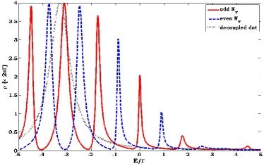
Figure 2: (Color online) LDOS’s for the dot. Solid (dashed) line represents the case with an odd (even) number of vortices in the superconductor. We take $\Gamma_{L}=\Gamma_{R}=\Gamma/2=0.5\pi v_{M}/L$, $\epsilon_{d}=-3.3\Gamma$, and $\bar{t}^{2}/v_{M}=2\Gamma$. The location of the peak will shift when a vortex is added or removed. For comparison, the dotted line corresponds to the case with $\bar{t}=0$.

A few remarks about $\rho(E)$ are in order. First of all, we notice that $\rho(-E,\epsilon_{d})=\rho(E,-\epsilon_{d})$. Consequently, $\rho(-E)=\rho(E)$ when $\epsilon_{d}=0$, as shown in the left diagram in Fig. 3. Next, $\rho(E)$ (or $A(E)$) is an oscillator function of $E$ on account of the coupling to the quantized energy levels of the chiral Majorana edge states. The location of the peak indicates the occurrence of a resonance, which depends on the number of vortices $N_{v}$ as well as the value of $\epsilon_{d}$. Variation of the value of $\bar{t}^{2}/v_{M}$ also slightly shifts the position of the resonance, but does not change the global feature significantly. For $\epsilon_{d}<0$ ($\epsilon_{d}>0$), most resonances have energies $E<0$ ($E>0$). Especially, a zero-energy resonance always exists when $N_{v}$ is odd, irrespective of the values of $\epsilon_{d}$ and $\bar{t}^{2}/v_{M}$. On the other hand, for an off-resonance dot, there is at least a resonance lying between $\epsilon_{d}$ and $0$ when $N_{v}$ is even.

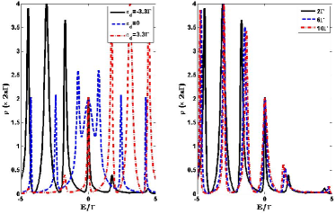
Figure 3: (Color online) LDOS’s for the dot with odd $N_{v}$. We take $\Gamma_{L}=\Gamma_{R}=\Gamma/2=0.5\pi v_{M}/L$. Left: $\rho(E)$ with $\bar{t}^{2}/v_{M}=2\Gamma$ for different values of $\epsilon_{d}$. The location of the resonance depends on the value of $\epsilon_{d}$ sensitively. Right: $\rho(E)$ with $\epsilon_{d}=-3.3\Gamma$ for different values of $\bar{t}^{2}/v_{M}$. The location of the resonance also slightly depends on the value of $\bar{t}^{2}/v_{M}$.

III.2 The differential conductance

Inserting Eq. (7) into Eq. (5), we obtain the differential conductance at zero temperature. The behavior of $G$ versus $eV$ is shown in Figs. 4 – 6. We see that $G$ depends on $N_{v}$. When $N_{v}$ is odd, a zero Majorana edge mode exists, which results in a zero-bias peak with the value $G/G_{0}=2\Gamma_{L}\Gamma_{R}/\Gamma^{2}$, even for an off-resonance dot. As noticed in the previous work on the topological superconducting nanowire,LB ; Vernek this is an indication of the existence of a zero-energy Majorana edge mode. For even $N_{v}$ such that no zero-energy edge modes exist in the TSC, the zero-bias conductance reaches the unitary value $G/G_{0}=4\Gamma_{L}\Gamma_{R}/\Gamma^{2}$ for an on-resonance dot. For an off-resonance dot, the conductance exhibits an oscillatory behavior as varying $eV$, and reaches half of the value in the unitary limit at the peak. Moreover, there is at least a conductance peak occurring at a value of $eV$ smaller than $2|\epsilon_{d}|$. These provide evidences for the coupling to quantized energy levels of chiral Majorana edge states. The positions of the conductance peaks shift by varying the gate voltage $V_{g}$, but are insensitive to the value of $\bar{t}^{2}/v_{M}$. For an on-resonance dot, i.e. $\epsilon_{d}=0$, a conductance peak with the value larger than $G/G_{0}=2\Gamma_{L}\Gamma_{R}/\Gamma^{2}$ occurs at a finite bias due to the enhanced side peaks in $\rho(E)$ (or $A(E)$) with odd $N_{v}$, as shown in the left diagram in Fig. 3. To sum up, the whole behavior of $G$ with varying $N_{v}$ and $eV$ as we have discussed is an indication of the existence of a chiral Majorana liquid at the edge of a TSC.

One may wonder how to distinguish the behavior of $G$ versus $eV$ for a dot side-coupled to a TSC from that for a multi-level dot. According to the above results, both are different in three respects. First of all, the conductance for a dot side-coupled to a TSC will shift upon adding or removing a vortex in the TSC, while the one for a dot decoupled to the TSC remains intact. Next, for an off-resonance dot, the value of the conductance peak in the present case is only half of the one in the unitary limit, whereas for a dot decoupled to the TSC, it will reach a non-universal value depending on the energy levels in the dot as long as $eV/2$ matches one level in the dot. Finally, for an on-resonance dot, the conductance peak in the present case will approach a universal value $G/G_{0}=2\Gamma_{L}\Gamma_{R}/\Gamma^{2}$ at large bias. In general, there is no such a behavior for a dot decoupled to the TSC.

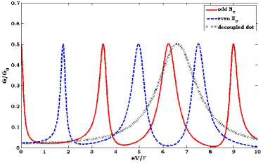
Figure 4: (Color online) The conductance (in units of $G_{0}$) versus $eV$ (in units of $\Gamma$). Solid (dashed) line represents the case with an odd (even) number of vortices in the superconductor. We take $\Gamma_{L}=\Gamma_{R}=\Gamma/2=0.5\pi v_{M}/L$, $\epsilon_{d}=-3.3\Gamma$, and $\bar{t}^{2}/v_{M}=2\Gamma$. For comparison, the dotted line corresponds to the case with $\bar{t}=0$.

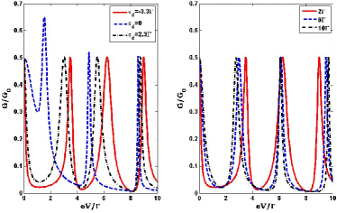
Figure 5: (Color online) The conductance (in units of $G_{0}$) versus $eV$ (in units of $\Gamma$) with odd $N_{v}$. We take $\Gamma_{L}=\Gamma_{R}=\Gamma/2=0.5\pi v_{M}/L$. Left: $G$ as a function of $eV$ with $\bar{t}^{2}/v_{M}=2\Gamma$ for different values of $\epsilon_{d}$. Right: $G$ as a function of $eV$ with $\epsilon_{d}=-3.3\Gamma$ for different values of $\bar{t}^{2}/v_{M}$.

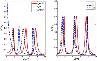
Figure 6: (Color online) The conductance (in units of $G_{0}$) versus $eV$ (in units of $\Gamma$) with even $N_{v}$. We take $\Gamma_{L}=\Gamma_{R}=\Gamma/2=0.5\pi v_{M}/L$. Left: $G$ as a function of $eV$ with $\bar{t}^{2}/v_{M}=2\Gamma$ for different values of $\epsilon_{d}$. Right: $G$ as a function of $eV$ with $\epsilon_{d}=-3.3\Gamma$ for different values of $\bar{t}^{2}/v_{M}$.

III.3 The Majorana-fermion representation

The above results can be understood by introducing the Majorana-fermion representation for the dot electrons:

$$\gamma_{1}=\frac{\xi d+\xi^{*}d^{\dagger}}{\sqrt{2}}\ ,~{}~{}\gamma_{2}=\frac{\xi d-\xi^{*}d^{\dagger}}{\sqrt{2}i}\ ,$$

where $\gamma_{i}$ satisfy the anticommutation relation

$$\{\gamma_{i},\gamma_{j}\}=\delta_{ij}\ ,$$

for $i,j=1,2$. We notice that only $\gamma_{1}$ couples to the chiral Majorana edge states directly. $\gamma_{2}$ couples the chiral Majorana edge states indirectly through the $\epsilon_{d}$ term, which represents the hopping between $\gamma_{1}$ and $\gamma_{2}$. The retarded Green functions for $\gamma_{i}$, which are defined as

$$iS_{j}^{r}(t_{1},t_{2})\equiv\Theta(t_{1}-t_{2})\langle\{\gamma_{j}(t_{1}),\gamma_{j}(t_{2})\}\rangle\ ,$$

are related to the two-point Green functions of the dot electrons through the following relations:

$$S_{1}^{r}(t_{1},t_{2}) = \frac{1}{2}\!\left[D_{r}(t_{1},t_{2})-D_{a}(t_{2},t_{1})\right]$$

$$+\frac{1}{2}\!\left[\xi^{2}F_{r}(t_{1},t_{2})+(\xi^{*})^{2}\tilde{F}_{r}(t_{1},t_{2})\right],$$

$$S_{2}^{r}(t_{1},t_{2}) = \frac{1}{2}\!\left[D_{r}(t_{1},t_{2})-D_{a}(t_{2},t_{1})\right]$$

$$-\frac{1}{2}\!\left[\xi^{2}F_{r}(t_{1},t_{2})+(\xi^{*})^{2}\tilde{F}_{r}(t_{1},t_{2})\right],$$

where

$$iF_{r}(t,t^{\prime}) \equiv \Theta(t-t^{\prime})\langle\{d(t),d(t^{\prime})\}\rangle\ ,$$

$$i\tilde{F}_{r}(t,t^{\prime}) \equiv \Theta(t-t^{\prime})\langle\{d^{\dagger}(t),d^{\dagger}(t^{\prime})\}\rangle\ ,$$

are anomalous Green functions for dot electrons. By taking the Fourier transform, we get

$$S_{1}^{r}(\omega)\!\!\! = \!\!\frac{1}{2}\!\left[D_{r}(\omega)-D_{a}(-\omega)+\xi^{2}F_{r}(\omega)+(\xi^{*})^{2}\tilde{F}_{r}(\omega)\right],$$

$$S_{2}^{r}(\omega)\!\!\! = \!\!\frac{1}{2}\!\left[D_{r}(\omega)-D_{a}(-\omega)-\xi^{2}F_{r}(\omega)-(\xi^{*})^{2}\tilde{F}_{r}(\omega)\right].~{}~{}~{}~{}$$ (8)

From Eq. (8), we find that

$$\frac{1}{2}[A(E)+A(-E)]=\pi[\rho_{1}(E)+\rho_{2}(E)]\ ,$$ (9)

where $\rho_{i}(E)=-\frac{1}{\pi}\mbox{Im}[S_{i}^{r}(E)]$ with $i=1,2$ are the LDOS’s for $\gamma_{1}$ and $\gamma_{2}$. That is, $G(V)$, in fact, measures the sum of the LDOS’s for $\gamma_{i}$.

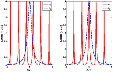
Figure 7: (Color online) LDOS’s for $\gamma_{1}$ and $\gamma_{2}$ with $\epsilon_{d}=0$. We take $\Gamma_{L}=\Gamma_{R}=\Gamma/2=0.5\pi v_{M}/L$ and $\bar{t}^{2}/v_{M}=2\Gamma$. Left: odd $N_{v}$. Right: even $N_{v}$.

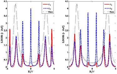
Figure 8: (Color online) LDOS’s for $\gamma_{1}$ and $\gamma_{2}$ with $\epsilon_{d}=-3.3\Gamma$. We take $\Gamma_{L}=\Gamma_{R}=\Gamma/2=0.5\pi v_{M}/L$ and $\bar{t}^{2}/v_{M}=2\Gamma$. Left: odd $N_{v}$. Right: even $N_{v}$. For comparison, the dotted line corresponds to the case with $\bar{t}=0$.

The anomalous Green functions for dot fermions can also be obtained by the method of EOM, yielding

$$F_{r}(\omega) = \frac{(\xi^{*})^{2}M(\omega)}{\left[\omega-M(\omega)+\frac{i}{2}\Gamma\right]^{2}\!-\epsilon_{d}^{2}-[M(\omega)]^{2}}\ ,$$

$$\tilde{F}_{r}(\omega) = \frac{\xi^{2}M(\omega)}{\left[\omega-M(\omega)+\frac{i}{2}\Gamma\right]^{2}\!-\epsilon_{d}^{2}-[M(\omega)]^{2}}\ .$$ (10)

Inserting Eqs. (6) and (10) into Eq. (8) gives

$$S_{1}^{r}(\omega) = \frac{\omega+\frac{i}{2}\Gamma}{\left[\omega-M(\omega)+\frac{i}{2}\Gamma\right]^{2}\!-\epsilon_{d}^{2}-[M(\omega)]^{2}}\ ,$$

$$S_{2}^{r}(\omega) = \frac{\omega-2M(\omega)+\frac{i}{2}\Gamma}{\left[\omega-M(\omega)+\frac{i}{2}\Gamma\right]^{2}\!-\epsilon_{d}^{2}-[M(\omega)]^{2}}\ .$$ (11)

Hence, the LDOS’s for $\gamma_{1}$ and $\gamma_{2}$ take the forms:

$$\rho_{1}(E)\!\!\! = \!\!\!\frac{\Gamma\!\left(E^{2}+\epsilon_{d}^{2}+\Gamma^{2}/4\right)/2\pi}{\left[E^{2}\!-\!2EM(E)\!-\!\epsilon_{d}^{2}\!+\!\frac{\Gamma^{2}}{4}\right]^{2}\!\!+\!\Gamma^{2}\!\!\left\{\epsilon_{d}^{2}\!+\![M(E)]^{2}\right\}},$$

$$\rho_{2}(E)\!\!\! = \!\!\!\frac{\Gamma\!\left\{[E-2M(E)]^{2}+\epsilon_{d}^{2}+\Gamma^{2}/4\right\}/2\pi}{\left[E^{2}\!-\!2EM(E)\!-\!\epsilon_{d}^{2}\!+\!\frac{\Gamma^{2}}{4}\right]^{2}\!\!+\!\Gamma^{2}\!\!\left\{\epsilon_{d}^{2}\!+\![M(E)]^{2}\right\}}.$$

We see that $\rho_{i}(E)$ with $i=1,2$ are even functions of $E$, i.e. $\rho_{i}(-E)=\rho_{i}(E)$, which arises from the fact that $\gamma_{i}$ are real fermions. The behaviors of $\rho_{i}(E)$ with $i=1,2$ are shown in Figs. 7 and 8.

For the on-resonance dot, i.e. $\epsilon_{d}=0$, we notice that $\gamma_{2}$ does not couple to the chiral Majorana edge states at all. Thus, its LDOS exhibits a Lorentzian form with a peak at zero energy and width determined by $\Gamma$, and is independent of the number of vortices in the TSC. On the other hand, due to the coupling to the chiral Majorana edge states, $\rho_{1}$ develops several peaks located at the values of $eV/\Gamma$ which are the real roots of the equation $x=2M(x)$, and the peak values are universal in the sense that $2\pi\Gamma(\rho_{1})_{\mbox{{\tiny max}}}=4$. Hence, the peak values of $G(V)/G_{0}$ (in units of $\Gamma_{L}\Gamma_{R}/\Gamma^{2}$) are nonuniversal, except that $G(0)/G_{0}=2\Gamma_{L}\Gamma_{R}/\Gamma^{2},4\Gamma_{L}\Gamma_{R}/\Gamma^{2}$ for odd and even $N_{v}$, respectively. Moreover, $G(V)/G_{0}$ approaches the value $2\Gamma_{L}\Gamma_{R}/\Gamma^{2}$ as $eV/\Gamma\gg 1$ since $\rho_{2}(E)\rightarrow 0$ when $E/\Gamma\gg 1/2$. On the other hand, $\rho_{1}$ becomes zero when $1/M(E)=0$ or $E=E_{l}$, where $E_{l}=\frac{2\pi v_{M}}{L}[l+(N_{v}+1)/2]$ with integer $l$ are the quantized energy levels of the chiral Majorana edge modes. This suggests that the coupling to the chiral Majorana edge states will suppress half of the degrees of freedom for the dot electrons for an on-resonance dot. One may view this as “Majorana-fermionization” of half of the degrees of freedom of dot electrons. In summary, on account of the oscillatory behavior of $\rho_{1}(E)$, which follows from the coupling to the chiral Majorana edge states, $G(V)$ for an on-resonance dot becomes an oscillating function of $eV$.

For an off-resonance dot, we notice that the suppression in $\rho_{1}$ also occurs whenever $E$ matches the quantized energy levels of the chiral Majorana edge modes. That is, $\rho_{1}(E)=0$ for $E=E_{l}$. This implies the robustness of “Majorana-fermionization” of dot electrons. Moreover, $\rho_{1}$ as well as $\rho_{2}$ are oscillatory functions of $E$ due to the coupling to the chiral Majorana edge states and $\epsilon_{d}\neq 0$. In fact, this oscillation is intimately related to the suppression in $\rho_{1}$ at $E=E_{l}$ since it must obey the sum rule:

$$\int^{+\infty}_{0}\!dE\rho_{1}(E)=\frac{1}{2}\ .$$

This results in the oscillatory behavior of $G(V)$ as varying $eV$. The peaks in $G(V)$ are located at the values of $eV/(2\Gamma)$ when they are the real roots of the equation $x^{2}-2M(x)x=(\epsilon_{d}/\Gamma)^{2}\pm 1/4$. Thus, $G(V)/G_{0}$ takes the universal value $2\Gamma_{L}\Gamma_{R}/\Gamma^{2}$ at these peaks.

IV Conclusion

To sum up, we study the electrical transport through a QD side-coupled to a TSC in the spinless regime. We pay attention to the behavior of the conductance $G$ as varying the bias $V$. We found that $G$ is an oscillatory function of $eV$ similar to the one for a multi-level dot. However, the function $G(V)$ in the present case is distinguished from that for a multi-level dot in three respects. First of all, the former will shift upon adding or removing a vortex in the TSC, while such an effect is not observed for the latter. Next, for an off-resonance dot, the value of the conductance peak in the former case is only half of the one in the unitary limit, whereas for the latter, it will reach a non-universal value depending on the energy levels in the dot as long as $eV/2$ matches one level in the dot. Finally, for an on-resonance dot, the conductance peak in the former case will approach a universal value $G/G_{0}=2\Gamma_{L}\Gamma_{R}/\Gamma^{2}$ at large bias. In general, there is no such a behavior for the latter. We consider these features the signatures of chiral Majorana edge states.

The oscillatory behavior of $G(V)$ can be understood by introducing the Majorana representation of dot electrons. The dot electron is composed of two Majorana fermions. Only one of them is coupled to the chiral Majorana edge states directly. We show that this coupling results in the suppression in the LDOS whenever the energy matches one of the quantized energy levels of the chiral Majorana edge states. This phenomenon is dubbed as Majorana fermionization because only the other Majorana fermion, which is not directly coupled to the chiral Majorana edge states, survives at these energies. It is interesting to explore similar phenomena in other situations.

Finally, we would like to emphasize that the above results are obtained assuming zero temperature and without other possible dissipations. Extension to the finite temperature can start with Eq. (4). Dissipations arising from the environment, however, involve the change of the model. Dissipation effects may suppress the tunneling rate or cause a nontrivial phase diagram such that the results obtained from the tunneling spectroscopy to identify the signature of the chiral Majorana liquid may be dubious. The effects of ohmic dissipations on the tunneling between the normal metallic lead and the end of a $1$D TSC has been studied,DL which shows distinct temperature behaviors for the zero-bias conductance peaks due to the Majorana fermion end mode and other effects. It deserves to include the dissipation effects into our analysis to see how the results we obtained are modified.

- (1) N. Read and D. Green, Phys. Rev. B 61, 10267 (2000).
- (2) V. Gurarie, L. Radzihovsky, and A.V. Andreev, Phys. Rev. Lett. 94, 230403 (2005).
- (3) M. Stone and S.B. Chung, Phys. Rev. B 73, 014505 (2006).
- (4) A.Y. Kitaev, Phys.-Usp. 44, 131 (2001).
- (5) D.A. Ivanov, Phys. Rev. Lett. 86, 268 (2001).
- (6) A.Y. Kitaev, Ann. Phys. (N.Y.) 303, 2 (2003).
- (7) C. Nayak, S.H. Simon, A. Stern, M. Freedman, and S. Das Sarma, Rev. Mod. Phys. 80, 1083 (2008).
- (8) R.M. Lutchyn, J.D. Sau, and S. Das Sarma, Phys. Rev. Lett. 105, 077001 (2010).
- (9) Y. Oreg, G. Refael, and F. von Oppen, Phys. Rev. Lett. 105, 177002 (2010).
- (10) V. Mourik, K. Zuo, S.M. Frolov, S.R. Plissard, E.P.A.M. Bakkers, and L.P. Kowenhoven, Science 336, 1003 (2012).
- (11) E.J.H. Lee, X.C. Jiang, M. Houzet, R. Aguado, C.M. Lieber, and S. De Franceschi, Nature Nano. 9, 79 (2014), which sheds some light on the controversy about the zero-bias anomaly and its relevancy on the signature of Majorana mode.
- (12) L. Fu and C.L. Kane, Phys. Rev. Lett. 100, 096407 (2008).
- (13) C.J. Bolech and E. Demler, Phys. Rev. Lett. 98, 237002 (2007).
- (14) J. Nilsson, A.R. Akhmerov, and C.W.J. Beenakker, Phys. Rev. Lett. 101, 120403 (2008).
- (15) K.T. Law, P.A. Lee, and T.K. Ng, Phys. Rev. Lett 103, 237001 (2009).
- (16) L. Fu and C.L. Kane, Phys. Rev. B 79, 161408(R) (2009).
- (17) K.T. Law and P.A. Lee, Phys. Rev. B 84, 081304(R) (2011).
- (18) P.A. Ioselevich and M.V. Feigelḿan, Phys. Rev. Lett. 106, 077003 (2011).
- (19) M. Leijnse and K. Flensberg, Phys. Rev. B 84, 140501(R) (2011).
- (20) D.E. Liu and H.U. Baranger, Phys. Rev. B 84, 201308(R) (2011).
- (21) E. Vernek, P.H. Penteado, A.C. Seridonio, and J.C. Egues, Phys. Rev. B 89, 165314 (2014).
- (22) Y. Cao, P. Wang, G. Xiong, M. Gong, and X.Q. Li, Phys. Rev. B 86, 115311 (2012).
- (23) L. Ponomarenko, F. Schedin, M.I. Katsnelson, R. Yang, E.W. Hill, K.S. Novoselov, and A.K. Geim, Science 320, 5874 (2008); J. Güttinger, C. Stampfer, F. Libisch, T. Frey, J. Burgdörfer, T. Ihn, and K. Ensslin, Phys. Rev. Lett. 103, 046810 (2009).
- (24) For a review, see, for example, S. Sapmaz, P. Jarillo-Herrero, L.P. Kouwenhoven, and H.S.J. van der Zant, Semicond. Sci. Technol. 21, S52 (2006).
- (25) J.G. Analytis, R.D. McDonald, S.C. Riggs, J.-H. Chu, G.S. Boebinger, and I.R. Fisher, Nature Phys. 6, 960 (2010); D.X. Qu, Y.S. Hor, J. Xiong, R.J. Cava, and N.P. Ong, Science 329, 821 (2010).
- (26) Within the context of our setup, the Kondo effect is not significant here. For the discussions on a magnetic impurity coupled to the helical Majorana liquid, i.e. the edge states of the time-reversal invariant TSC, see, for example, R. itko and P. Simon, Phys. Rev. B 84, 195310 (2011). For a discussion on the interplay between the Kondon effect and the Majorana-induced couplings in a QD coupled to the end of a D TSC, see, for example, Y. Avishai, Phys. Rev. Lett. 107, 176802 (2011) and M. Cheng, M. Becker, B. Bauer, and R.M. Lutchyn, arXiv: 1308.4156. See also H. Khim, R. Lpez, J.S. Lim, and M. Lee, arXiv: 1408.5053 for the study on the thermoelectric response of a Konod dot side-coupled to the Majorana fermion at the end of a D TSC.
- (27) Y. Meir and N.S. Wingreen, Phys. Rev. Lett. 68, 2512 (1992).
- (28) D.E. Liu, Phys. Rev. Lett. 111, 207003 (2013).