Preference Networks: Probabilistic Models for Recommendation Systems

Abstract

Recommender systems are important to help users select relevant and personalised information over massive amounts of data available. We propose an unified framework called Preference Network (PN) that jointly models various types of domain knowledge for the task of recommendation. The PN is a probabilistic model that systematically combines both content-based filtering and collaborative filtering into a single conditional Markov random field. Once estimated, it serves as a probabilistic database that supports various useful queries such as rating prediction and top-$N$ recommendation. To handle the challenging problem of learning large networks of users and items, we employ a simple but effective pseudo-likelihood with regularisation. Experiments on the movie rating data demonstrate the merits of the PN.

Keywords: Hybrid Recommender Systems, Collaborative Filtering, Preference Networks, Conditional Markov Networks, Movie Rating.

1 Introduction

With the explosive growth of the Internet, users are currently overloaded by massive amount of media, data and services. Thus selective delivery that matches personal needs is very critical. Automated recommender systems have been designed for this purpose, and they are deployed in major online stores such as Amazon [http://www.amazon.com], Netflix [http://www.netfix.com] and new services such as Google News [http://news.google.com].

Two most common tasks in recommender systems are predicting the score the user might give for a product (the rating prediction task), and recommending a ranked list of most relevant items (the top-$N$ recommendation task). The recommendations are made on the basis of the content of products and services (content-based), or based on collective preferences of the crowd (collaborative filtering), or both (hybrid methods). Typically, content-based methods work by matching product attributes to user-profiles using classification techniques. Collaborative filtering, on the other hand, relies on preferences over a set products that a given user and others have expressed. From the preferences, typically in term of numerical ratings, correlation-based methods measure similarities between users Resnick et al. (1994) (user-based methods) and products Sarwar et al. (2001) (item-based methods). As content and preferences are complementary, hybrid methods often work best when both types of information is available Balabanović and Shoham (1997); Basu et al. (1998); Pazzani (1999); Schein et al. (2002); Basilico and Hofmann (2004).

Probabilistic modeling Breese et al. (1998); Heckerman et al. (2001); Hofmann (2004); Marlin (2004) has been applied to the recommendation problem to some degree and their success has been mixed. Generally, they build probabilistic models that explain data. Earlier methods include Bayesian networks and dependency networks Breese et al. (1998); Heckerman et al. (2001) have yet to prove competitive against well-known correlation-based counterparts. The more recent work attempts to perform clustering. Some representative techniques are mixture models, probabilistic latent semantic analysis (pLSA) Hofmann (2004) and latent Dirichlet allocation (LDA) Marlin (2004). These methods are generative in the sense that it assumes some hidden process that generates observed data such as items, users and ratings. The generative assumption is often made for algorithmic convenience and but it does not necessarily reflect the true process of the real data.

Machine learning techniques Billsus and Pazzani (1998); Basu et al. (1998); Basilico and Hofmann (2004) address the rating prediction directly without making the generative assumption. Rather, they map the recommendation into a classification problem that existing classifiers can solve Basu et al. (1998); Zhang and Iyengar (2002). The map typically considers each user or each item as an independent problem, and ratings are training instances. However, the assumption that training instances are independently generated does not hold in collaborative filtering. Rather all the ratings are interconnected directly or indirectly through common users and items.

To sum up, it is desirable to build a recommendation system that can seamlessly integrate content and correlation information in a disciplined manner. At the same time, the system should address the prediction and recommendation tasks directly without replying on strong prior assumptions such as generative process and independence. To that end, we propose a probabilistic graphical formulation called Preference Network (PN) that has these desirable properties. The PN is a graph whose vertexes represent ratings (or preferences) and edges represent dependencies between ratings. The networked ratings are treated as random variables of conditional Markov random fields Lafferty et al. (2001). Thus the PN is a formal and expressive formulation that supports learning from existing data and various inference tasks to make future prediction and recommendation. The probabilistic dependencies between ratings capture the correlations between co-rating users (as used in Resnick et al. (1994)) and between co-rated items (as used in Sarwar et al. (2001)).

Different from previous probabilistic models, the PN does not make any generative assumption. Rather, prediction of preferences is addressed directly based on the content and prior ratings available in the database. It also avoids the independence assumption made in the standard machine learning approach by supporting collective classification of preferences. The nature of graphical modeling enables PN to support missing ratings and joint predictions for a set of items and users. It provides some measure of confidence in each prediction made, making it easy to assess the nature of recommendation and rank results. More importantly, our experiments show that the PNs are competitive against the well-known user-based method Resnick et al. (1994) and the item-based method Sarwar et al. (2001).

2 Recommender Systems

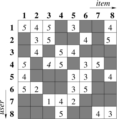
Figure 1: Preference matrix. Entries are numerical rating (or preference) and empty cells are to be filled by the recommender system.

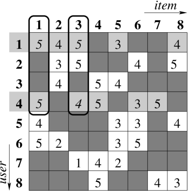
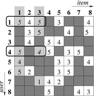
(a)	(b)

Figure 2: User-based correlation (a) and Item-based correlation (b).

This section provides some background on recommender systems and we refer readers to Adomavicius and Tuzhilin (2005) for a more comprehensive survey. Let us start with some notations. Let $\mathcal{U}=\{u_{1},\ldots,u_{M}\}$ be the set of $M$ users (e.g. service subscribers, movie viewers, Website visitors or product buyers), and $\mathcal{I}=\{i_{1},\ldots,i_{L}\}$ be the set of $L$ products or items (e.g. services, movies, Webpages or books) that the user can select from. Let us further denote $\mathcal{M}=\{r_{ui}\}$ the preference matrix where $u$ is the user index, $i$ is the item index, and $r_{ui}$ is the preference or the numerical rating of user $u$ over item $i$ (see Figure 1 for an illustration). In this paper, we assume that ratings have been appropriately transformed into integers, i.e. $r_{ui}\in\{1,2,...,S\}$.

Typically, a user usually rates only a small number of items and thus making the preference matrix $\mathcal{M}$ extremely sparse. For example, in the MovieLens dataset that we use in our experiments (Section 4), only about 6.3% entries in the $\mathcal{M}$ matrix are filled, and in large e-commerce sites, the sparsity can be as small as 0.001%. The rating prediction task in recommender systems can be considered as filling the empty cells in the preference matrix. Of course, due to the data sparsity, filling all the cells is impractical and often unnecessary because each user will be interested in a very small set of items. Rather, it is only appropriate for a limited set of entries in each row (corresponding to a user). Identifying the most relevant entries and ranking them are the goal of top-$N$ recommendation.

Recommender techniques often fall into three groups: content-based, collaborative filtering, and hybrid methods that combines the former two groups.

Content-based methods rely on the content of items that match a user’s profile to make recommendation using some classification techniques (e.g. see Mooney and Roy (2000)). The content of an item is often referred to the set of attributes that characterise it. For example, in movie recommendation, item attributes include movie genres, release date, leading actor/actress, director, ratings by critics, financial aspects, movie description and reviews. Similarly, user attributes include static information such as age, sex, location, language, occupation and marriage status and dynamic information such as watching time (day/night/late night), context of use (e.g. home/theater/family/dating/group/company), and in case of on-demand videos, what other TV channels are showing, what the person has been watching in the past hours, days or weeks.

Collaborative filtering takes a different approach in that recommendation is based not only on the usage history of the user but also on experience and wisdom of related people in the user-item network. Most existing algorithms taking some measure of correlation between co-rating users or co-rated items. One family, known as user-based (sometimes memory-based) methods Resnick et al. (1994), predicts a new rating of an item based on existing ratings on the same item by other users:

$$r_{ui}=\bar{r}_{u}+\frac{\sum_{v\in U(i)}s(u,v)(r_{ui}-\bar{r}_{v})}{\sum_{v\in U(i)}|s(u,v)|}$$

where $s(u,v)$ is the similarity between user $u$ and user $v$, $U(i)$ is the set of all users who rate item $i$, and $\bar{r}_{u}$ is the average rating by user $u$. The similarity $s(u,v)$ is typically measured using Pearson’s correlation:

$$\frac{\sum_{i\in I(u,v)}(r_{ui}-\bar{r}_{u})(r_{vi}-\bar{r}_{v})}{\left[\sum_{i\in I(u,v)}(r_{ui}-\bar{r}_{u})^{2}\right]^{\frac{1}{2}}\left[\sum_{j\in I(u,v)}(r_{vj}-\bar{r}_{v})^{2}\right]^{\frac{1}{2}}}$$

where $I(u,v)$ is the set of all items co-rated by users $u$ and $v$. See Figure 2a for illustration. This similarity is computed offline for every pair of users who co-rate at least one common item.

The main drawback of user-based methods is in its lack of efficiency at prediction time because each prediction require searching and summing over all users who rate the current item. The set of such users is often very large for popular items, sometimes including all users in the database. In contrast, each user typically rates only a very limited number of items. Item-based methods Sarwar et al. (2001) exploit that fact by simply exchanging the role of user and item in the user-based approach. Similarity between items $s(i,j)$ can be computed in several ways including the (adjusted) cosine between two item vectors, and the Pearson correlation. For example, the adjusted cosine similarity is computed as

$$\frac{\sum_{u\in U(i,j)}(r_{ui}-\bar{r}_{u})(r_{uj}-\bar{r}_{u})}{\left[{\sum_{u\in U(i,j)}(r_{ui}-\bar{r}_{u})^{2}}\right]^{\frac{1}{2}}\left[{\sum_{v\in U(i,j)}(r_{vj}-\bar{r}_{v})^{2}}\right]^{\frac{1}{2}}}$$

where $U(i,j)$ is the set of all users who co-rate both items $i$ and $j$. See Figure 2b for illustration. The new rating is predicted as

$$r_{ui}=\bar{r}_{i}+\frac{\sum_{j\in I(u)}s(i,j)(r_{uj}-\bar{r}_{j})}{\sum_{j\in I(u)}|s(i,j)|}$$

where $I(u)$ is the set of items rated by user $u$.

Many other methods attempt to build a model of training data that then use the model to perform prediction on unseen data. One class of methods employ probabilistic graphical models such as Bayesian networks Breese et al. (1998), dependency networks Heckerman et al. (2001), and restricted Boltzmann machines Salakhutdinov et al. (2007). Our proposed method using Markov networks fall under the category of undirected graphical models. It resembles dependency networks in the way that pseudo-likelihood Besag (1974) learning is employed, but dependency networks are generally inconsistent probabilistic models. In Salakhutdinov et al. (2007), the authors build a generative Boltzmann machine for each user with hidden variables, while our method constructs a single discriminative Markov network for the whole database of all ratings.

Much of other probabilistic work attempts to perform clustering. This is an important technique for reducing the dimensionality and noise, dealing with data sparsity and more significantly, discovering latent structures. Here the latent structures are either communities of users with similar tastes or categories of items with similar features. Some representative techniques are mixture models, probabilistic latent semantic analysis (pLSA) Hofmann (2004) and latent Dirichlet allocation (LDA) Marlin (2004). These methods try to uncover some hidden process which is assumed to generate items, users and ratings. In our approach, no such generation is assumed and ratings are modeled conditionally given items and users and prior knowledge.

Statistical machine learning techniques Billsus and Pazzani (1998); Basu et al. (1998); Zhang and Iyengar (2002); Basilico and Hofmann (2004); Zitnick and Kanade (2004) have also been used to some extent. One of the key observations made is that there is some similarity between text classification and rating prediction Zhang and Iyengar (2002). However, the main difficulty is that the features in collaborative filtering are not rich and the nature of prediction is different. There are two ways to convert collaborative filtering into a classification problem Billsus and Pazzani (1998). The first is to build a model for each item, and ratings by different users are treated as training instances. The other builds a model for each user, and ratings on different items by this user are considered as training instances Breese et al. (1998). These treatments, however, are complementary, and thus, there should be a better way to systematically unify them Basu et al. (1998); Basilico and Hofmann (2004). That is, the pairs (user,item) are now as independent training instances. Our approach, on the other hand, considers the pair as just a node in the network, thus relaxing the independence assumption.

Hybrid methods exploit the fact that content-based and collaborative filtering methods are complementary Balabanović and Shoham (1997); Basu et al. (1998); Pazzani (1999); Schein et al. (2002); Basilico and Hofmann (2004). For example, the content-based methods do not suffer from the so-called cold-start problem Schein et al. (2002) in standard collaborative filtering. The situation is when new user and new item are introduced to the database, as no previous ratings are available, purely correlation-based methods cannot work. On the other hand, content information available is sometimes very limited to basic attributes that are shared by many items or users. Prediction by pure content-based methods in that case cannot be personalised and may be inaccurate. Some work approaches the problem by making independent predictions separately using a content-based method and a collaborative filtering method and then combining the results Claypool et al. (1999). Others (e.g. Basilico and Hofmann (2004)) create joint representation of content and collaborative features. We follow the latter approach.

3 Preference Networks for Hybrid Recommendation

3.1 Model Description

Let us start with the preference matrix $\mathcal{M}=\{r_{ui}\}$ discussed previously (cf. Sec. 2), where we treat each entry $r_{ui}$ in $\mathcal{M}$ as a random variable, and thus ideally we would be interested in a single joint model over $KM$ variables for both the learning phase and the prediction/recommendation phase. However, in practice, $KM$ is extremely large (e.g., $10^{6}\times 10^{6}$) making computation intractable. In addition, such a modeling is unncessary, because, as we have mentioned earlier in Section 2, a user is often interested in a moderate number of items. As a result, we adopt a two-step strategy. During the learning phase, we limit to model the joint distribution over existing ratings. And then during the prediction/recommendation phase, we extend the model to incoporate to-be-predicted entries.

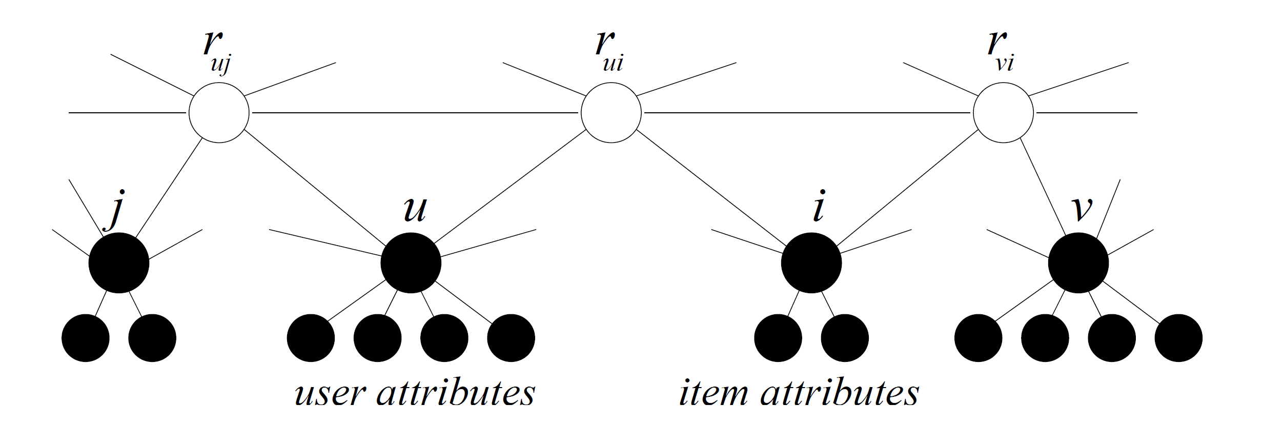
Figure 3: A fragment of the Preference Network.

We build the model by first representing the ratings and their relations using an undirected graph and then defining a joint distribution over the graph. Denote by $\mathcal{G}=(\mathcal{V},\mathcal{E})$ an undirected graph that has a set of vertexes $\mathcal{V}$ and a set of edges $\mathcal{E}$. Each vertex in $\mathcal{V}$ in this case represents a rating $r_{ui}$ of user $u$ over item $i$ and each edge in $\mathcal{E}$ capture a relation between two ratings. The set $\mathcal{E}$ defines a topological structure for the network, and specify how ratings are related.

We define the edges as follows. There is an edge between any two ratings by the same user, and an edge between two ratings on the same item. As a result, a vertex of $r_{ui}$ will be connected with $U(i)+I(u)-2$ other vertices. Thus, for each user, there is a fully connected subnetwork of all ratings she has made, plus connections to ratings by other users on these items. Likewise, for each item, there is a fully connected subnetwork of all ratings by different users on this item, plus connections to ratings on other items by these users. The resulting network $\mathcal{G}$ is typically very densely connected because $U(i)$ can be potentially very large (e.g. $10^{6}$).

Let us now specify the probabilistic modeling of the ratings and their relations that respect the graph $\mathcal{G}$. Denote $t=(u,i)$ and let $\mathcal{T}=\{t\}$ be the set of a pair index (user, item), which corresponds to entries used in each phase. For notation convenience let $X=\{r_{ui}\mid(u,i)\in\mathcal{T}\}$ denote the joint set of all variables, and the term ‘preference’ and ‘rating’ will be used exchangeably. When there is no confusion, we use $r_{u}$ to denote ratings related to user $u$ and $r_{i}$ denotes ratings related to item $i$.

In our approach to the hybrid recommendation task, we consider attributes of items $\{\mathbf{a}_{i}\}_{i=1}^{L}$, and attributes of users $\{\mathbf{a}_{u}\}_{i=u}^{M}$. Let $\mathbf{o}=\{\{\mathbf{a}_{i}\}_{i=1}^{L},\{\mathbf{a}_{u}\}_{i=u}^{M}\}$, we are interested in modeling the conditional distribution $P(X|\mathbf{o})$ of all user ratings $X$ given $\mathbf{o}$. We employ the conditional Markov random field Lafferty et al. (2001) as the underlying inference machinery. As $X$ collectively represents users’ preferences, we refer this model as Preference Network.

Preference Network (PN) is thus a conditional Markov random field that defines a distribution $P(X|\mathbf{o})$ over the graph $\mathcal{G}$:

$$P(X|\mathbf{o}) = \frac{1}{Z(\mathbf{o})}\Psi(X,\mathbf{o}),\quad\mbox{where}$$

$$\Psi(X,\mathbf{o}) = \prod_{t\in\mathcal{V}}\psi_{t}(r_{t},\mathbf{o})\prod_{(t,t^{\prime})\in\mathcal{E}}\psi_{t,t^{\prime}}(r_{t},r_{t^{\prime}},\mathbf{o})$$ (1)

where $Z(\mathbf{o})$ is the normalisation constant to ensure that $\sum_{X}P(X|\mathbf{o})=1$, and $\psi(.)$ is a positive function, often known as potential. More specifically, $\psi_{t}(r_{t},\mathbf{o})$ encodes the content information associated with the rating $r_{t}$ including the attributes of the user and the item. On the other hand, $\psi_{t,t^{\prime}}(r_{t},r_{t^{\prime}},\mathbf{o})$ captures the correlations between two ratings $r_{t}$ and $r_{t^{\prime}}$. Essentially, when there are no correlation potentials, the model is purely content-based, and when there are no content potentials, the model is purely collborative-filtering. Thus the PN integrates both types of recommendation in a seamlessly unified framework.

The contribution of content and correlation potentials to the joint distribution will be adjusted by weighting parameters associated with them. Specifically, the parameters are encoded in potentials as follows

$$\psi_{t}(r_{t},\mathbf{o}) = \exp\left\{\mathbf{w}_{v}^{\top}\mathbf{f}_{v}(r_{t},\mathbf{o})\right\}$$ (2)

$$\psi_{t,t^{\prime}}(r_{t},r_{t^{\prime}},\mathbf{o}) = \exp\left\{\mathbf{w}_{e}^{\top}\mathbf{f}_{e}(r_{t},r_{t^{\prime}},\mathbf{o})\right\}$$ (3)

where $\mathbf{f}(.)$ is the feature vector and $\mathbf{w}$ is the corresponding weight vector. Thus together with their weights, the features realise the contribution of the content and the strength of correlations between items and users. The design of features will be elaborated further in Section 3.2. Parameter estimation is described in Section 3.3.

3.2 Feature Design and Selection

Corresponding to the potentials in Equations 2 and 3, there are attribute-based features and correlation-based features. Attribute-based features include user/item identities and contents.

Identity Features. Assume that the ratings are integer, ranging from 1 to $S$. We know from the database the average rating $\bar{r}_{i}$ of item $i$ which roughly indicates the general quality of the item with respect to those who have rated it. Similarly, the average rating $\bar{r}_{u}$ by user $u$ over items she has rated roughly indicates the user-specific scale of the rating because the same rating of $4$ may mean ‘OK’ for a regular user, but may mean ‘excellent’ for a critic. We use two features item-specific $f_{i}(r_{ui},i)$ and user-specific $f_{u}(r_{ui},u)$:

$$f_{i}(r_{ui},i)=g(|r_{ui}-\bar{r}_{i}|),\quad f_{u}(r_{ui},u)=g(|r_{ui}-\bar{r}_{u}|)$$

where $g(\alpha)=1-\alpha/(S-1)$ is used to ensure that the feature values is normalized to $[0,1]$, and when $\alpha$ plays the role of rating deviation, $g(\alpha)=1$ for $\alpha=0$.

Content Features. For each rating by user $u$ on item $i$, we have a set of item attributes $\mathbf{a}_{i}$ and set of user attributes $\mathbf{a}_{u}$. Mapping from item attributes to user preference can be carried out through the following feature

$$\mathbf{f}_{u}(r_{ui})=\mathbf{a}_{i}g(|r_{ui}-\bar{r}_{u}|)$$

Similarly, we are also interested in seeing the classes of users who like a given item through the following mapping

$$\mathbf{f}_{i}(r_{ui})=\mathbf{a}_{u}g(|r_{ui}-\bar{r}_{i}|)$$

Correlation Features. We design two features to capture correlations between items or users. Specifically, the item-item $f_{i,j}(\cdot)$ features capture the fact that if a user rates two items then after offsetting the goodness of each item, the ratings may be similar

$$f_{i,j}(r_{ui},r_{uj}) = g(|(r_{ui}-\bar{r}_{i})-(r_{uj}-\bar{r}_{j})|)$$

Likewise, the user-user $f_{u,v}(\cdot)$ features capture the idea that if two users rate the same item then the ratings, after offset by user’s own scale, should be similar:

$$f_{u,v}(r_{ui},r_{vi}) = g(|(r_{ui}-\bar{r}_{u})-(r_{vi}-\bar{r}_{v})|)$$

Since the number of correlation features can be large, making model estimation less robust, we select only item-item features with positive correlation (given in Equation 2), and user-user features with positive correlations (given in Equation 2).

3.3 Parameter Estimation

Since the network is densely connected, learning methods based on the standard log-likelihood $\log P(X|\mathbf{o})$ are not applicable. This is because underlying inference for computing the log-likelihood and its gradient is only tractable for simple networks with simple chain or tree structures Pearl (1988). As a result, we resort to the simple but effective pseudo-likelihood learning method Besag (1974). Specifically, we replace the log likelihood by the regularised sum of log local likelihoods

$$\mathcal{L}(\mathbf{w})=\sum_{(u,i)\in\mathcal{T}}\log P(r_{ui}|\mathcal{N}(u,i),\mathbf{o})-\frac{1}{2}\bar{\mathbf{w}}^{\top}\bar{\mathbf{w}}$$ (4)

where, $\mathcal{N}(u,i)$ is the set of neighbour ratings that are connected to $r_{ui}$. As we mentioned earlier, the size of the neighbourhood is $|\mathcal{N}(u,i)|=U(i)+I(u)-2$. In the second term in the RHS, $\bar{\mathbf{w}}=\mathbf{w}/\boldsymbol{\sigma}$ (element-wise division, regularised by a prior diagonal Gaussian of mean $0$ and standard deviation vector $\boldsymbol{\sigma}$).

Finally, the parameters are estimated by maximising the pseudo-likelihood

$$\hat{\mathbf{w}}=\arg\max_{\mathbf{w}}\mathcal{L}(\mathbf{w})$$ (5)

Not only is this regularised pseudo-likelihood simple to implement, it makes sense since the local conditional distribution $P(r_{ui}|\mathcal{N}(u,i),\mathbf{o})$ is used in prediction (Equation 7). We limit ourselves to supervised learning in that all the ratings $\{r_{ui}\}$ in the training data are known. Thus, $\mathcal{L}(\mathbf{w})$ is a concave function of $\mathbf{w}$, and thus has a unique maximum.

To optimise the parameters, we use a simple stochastic gradient ascent procedure that updates the parameters after passing through a set of ratings by each user:

$$\mathbf{w}_{u}\leftarrow\mathbf{w}_{u}+\lambda\nabla\mathcal{L}(\mathbf{w}_{u})$$ (6)

where $\mathbf{w}_{u}$ is the subset of parameters that are associated with ratings by user $u$, and $\lambda>0$ is the learning rate. Typically, 2-3 passes through the entire data are often enough in our experiments. Further details of the computation are included in Appendix A.

3.4 Preference Prediction

Recall from Section 3.1 that we employ a two-step modeling. In the learning phase (Section 3.3), the model includes all previous ratings. Once the model has been estimated, we extend the graph structure to include new ratings that need to be predicted or recommended. Since the number of ratings newly added is typically small compared to the size of existing ratings, it can be assumed that the model parameters do not change.

The prediction of the rating $r_{ui}$ for user $u$ over item $i$ is given as

$$\hat{r}_{ui}=\arg\max_{r_{ui}}P(r_{ui}\mid\mathcal{N}(u,i),\mathbf{o})$$ (7)

The probability $P(\hat{r}_{ui}|\mathcal{N}(r_{ui}),\mathbf{o})$ is the measure of the confidence or ranking level in making this prediction. This can be useful in practical situations when we need high precision, that is, only ratings with the confidence above a certain threshold are presented to the users.

We can jointly infer the ratings $r_{u}$ of given user $u$ on a subset of items $\mathbf{i}=(i_{1},i_{2},..)$ as follows

$$\hat{r}_{u}=\arg\max_{r_{u}}P(r_{u}\mid\mathcal{N}(u),\mathbf{o})$$ (8)

where $\mathcal{N}(u)$ is the set of all existing ratings that share the common cliques with ratings by user $u$. In another scenario, we may want to recommend a relatively new item $i$ to a set of promising users, we can make joint predictions $r_{i}$ as follows

$$\hat{r}_{i}=\arg\max_{r_{i}}P(r_{i}\mid\mathcal{N}(i),\mathbf{o})$$ (9)

where $\mathcal{N}(i)$ is the set of all existing ratings that share the common cliques with ratings of item $i$. It may appear non-obvious that a prediction may depend on unknown ratings (other predictions to be made) but this is the advantage of the Markov networks. However, joint predictions for a user are only possible if the subset of items is small (e.g. less than 20) because we have a completely connected subnetwork for this user. This is even worse for joint prediction of an item because the target set of users is usually very large.

3.5 Top-$N$ recommendation

In order to provide a list of top-$N$ items to a given user, the first step is usually to identify a candidate set of $C$ promising items, where $C\geq N$. Then in the second step, we rank and choose the best $N$ items from this candidate set according to some measure of relevance.

Identifying the candicate set.
This step should be as efficient as possible and $C$ should be relatively small compared to the number of items in the database. There are two common techniques used in user-based and item-based methods, respectively. In the user-based technique, first we idenfify a set of $K$ most similar users, and then take the union of all items co-rated by these $K$ users. Then we remove items that the user has previously rated. In the item-based technique Deshpande and Karypis (2004), for each item the user has rated, we select the $K$ best similar items that the user has not rated. Then we take the union of all of these similar items.

Indeed, if $K\rightarrow\infty$, or equivalently, we use all similar users and items in the database, then the item sets returned by the item-based and user-based techniques are identical. To see why, we show that every candidate $j$ returned by the item-based technique is also the candidate by the user-based techqnique, and vice versa. Recall that a pair of items is said to be similar if they are jointly rated by the same user. Let $I(u)$ be the set of items rated by the current user $u$. So for each item $j\notin I(u)$ similar to item $i\in I(u)$, there must exist a user $v\neq u$ so that $i,j\in I(v)$. Since $u$ and $v$ jointly rate $i$, they are similar users, which mean that $j$ is also in the candidate set of the user-based method. Analogously, for each candidate $j$ rated by user $v$, who is similar to $u$, and $j\notin I(u)$, there must be an item $i\neq j$ jointly rated by both $u$ and $v$. Thus $i,j\in I(v)$, and therefore they are similar. This means that $j$ must be a candidate by the item-based technique.

In our Preference Networks, the similarity measure is replaced by the correlation between users or between items. The correlation is in turn captured by the corresponding correlation parameters. Thus, we can use either the user-user correlation or item-item correlation to identify the candicate set. Furthermore, we can also use both the correlation types and take the union of the two candidate sets.

Ranking the candidate set.
The second step in the top-$N$ recommendation is to rank these $C$ candicates according to some scoring methods. Ranking in the user-based methods is often based on item popularity, i.e. the number of users in the neighbourhood who have rated the item. Ranking in the item-based methods (Deshpande and Karypis, 2004) is computed by considering not only the number of raters but the similarity between the items being ranked and the set of items already rated by the user.

Under our Preference Networks formulation, we propose to compute the change in system energy and use it as ranking measure. Our PN can be thought as a stochastic physical system whose energy is related to the conditional distribution as follows

$$P(X|\mathbf{o})=\frac{1}{Z(\mathbf{o})}\exp(-E(X,\mathbf{o}))$$ (10)

where $E(X,\mathbf{o})=-\log\Psi(X,\mathbf{o})$ is the system energy. Thus the lower energy the system state $X$ has, the more probable the system is in that state. Let $t=(u,i)$, from Equations 2 and 3, we can see that the system energy is the sum of node-based energy and interaction energy

$$E(X,\mathbf{o}) = \sum_{t\in\mathcal{V}}E(r_{t},\mathbf{o})+\sum_{(t,t^{\prime})\in\mathcal{E}}E(r_{t},r_{t^{\prime}}\mathbf{o})$$

where

$$E(r_{t},\mathbf{o}) = -{\mathbf{w}}_{v}^{\top}{\mathbf{f}}_{v}(r_{t},\mathbf{o})$$ (11)

$$E(r_{t},r_{t^{\prime}},\mathbf{o}) = -{\mathbf{w}}_{e}^{\top}{\mathbf{f}}_{e}(r_{t},r_{t^{\prime}},\mathbf{o})$$ (12)

Recommending a new item $i$ to a given user $u$ is equivalent to extending the system by adding new rating node $r_{ui}$. The change in system energy is therefore the sum of node-based energy of the new node, and the interation energy between the node and its neighbours.

$$\Delta E({r}_{t},\mathbf{o})=E({r}_{t},\mathbf{o})+\sum_{t^{\prime}\in\mathcal{N}(t)}E({r}_{t},r_{t^{\prime}},\mathbf{o})$$

For simplicity, we assume that the state of the existing system does not change after node addition. Typically, we want the extended system to be in the most probable state, or equivalently the system state with lowest energy. This means that the node that causes the most reduction of system energy will be prefered. Since we do not know the correct state $r_{t}$ of the new node $t$, we may guess by predicting $\hat{r}_{t}$ using Equation 7. Let us call the energy reduction by this method the maximal energy change. Alternatively, we may compute the expected energy change to account for the uncertainty in the preference prediction

$$\mathbb{E}[\Delta E(r_{t},\mathbf{o})]=\sum_{r_{t}}P(r_{t}|\mathcal{N}(t),\mathbf{o})\Delta E(r_{t},\mathbf{o})$$ (13)

4 Experiments

In this section, we evaluate our Preference Network against well-established correlation methods on the movie recommendation tasks, which include rate prediction and top-$N$ item recommendation.

4.1 Data and Experimental Setup

We use the MovieLens data, collected by the GroupLens Research Project at the University of Minnesota from September 19th, 1997 through April 22nd, 1998. We use the dataset of 100,000 ratings in the 1-5 scale. This has 943 users and 1682 movies. The data is divided into a training set of 80,000 ratings, and the test set of 20,000 ratings. The training data accounts for 852,848 and 411,546 user-based item-based correlation features.

We transform the content attributes into a vector of binary indicators. Some attributes such as sex are categorical and thus are dimensions in the vector. Age requires some segmentation into intervals: under 18, 18-24, 25-34, 35-44, 45-49, 50-55, and 56+. We limit user attributes to age, sex and 20 job categories , and item attributes to 19 film genres . Much richer movie content can be obtained from the Internet Movie Database (IMDB).

4.2 Accuracy of Rating Prediction

In the training phrase, we set the learning rate $\lambda=0.001$ and the regularisation term $\sigma=1$. We compare our method with well-known user-based Resnick et al. (1994) and item-based Sarwar et al. (2001) techniques (see Section 2). Two metrics are used: the mean absolute error (MAE)

$$\sum_{(u,i)\in\mathcal{T}^{\prime}}|\hat{r}_{ui}-r_{ui}|/(|\mathcal{T}^{\prime}|)$$ (14)

where $\mathcal{T}^{\prime}$ is the set of rating indexes in the test data, and the mean 0/1 error

$$\sum_{(u,i)\in\mathcal{T}^{\prime}}\delta(\hat{r}_{ui}\neq r_{ui})/(|\mathcal{T}^{\prime}|)$$ (15)

In general, the MAE is more desirable than the 0/1 error because making exact prediction may not be required and making ‘closed enough’ predictions is still helpful. As item-based and user-used algorithms output real ratings, we round the numbers before computing the errors. Results shown in Figure 4 demonstrate that the PN outperforms both the item-based and user-based methods.

Sensitivity to Data Sparsity.
To evaluate methods against data sparsity, we randomly subsample the training set, but fix the test set. We report the performance of different methods using the MAE metric in Figure 5 and using the mean 0/1 errors in Figure 6. As expected, the purely content-based method deals with the sparsity in the user-item rating matrix very well, i.e. when the training data is limited. However, as the content we use here is limited to a basic set of attributes, more data does not help the content-based method further. The correlation-based method (purely collaborative filtering), on the other hand, suffers severely from the sparsity, but outperforms all other methods when the data is sufficient. Finally, the hybrid method, which combines all the content, identity and correlation features, improves the performance of all the component methods, both when data is sparse, and when it is sufficient.

Figure 4: The mean absolute error of recommendation methods (Item: item-based method, and Item-R: item-based method with rounding).

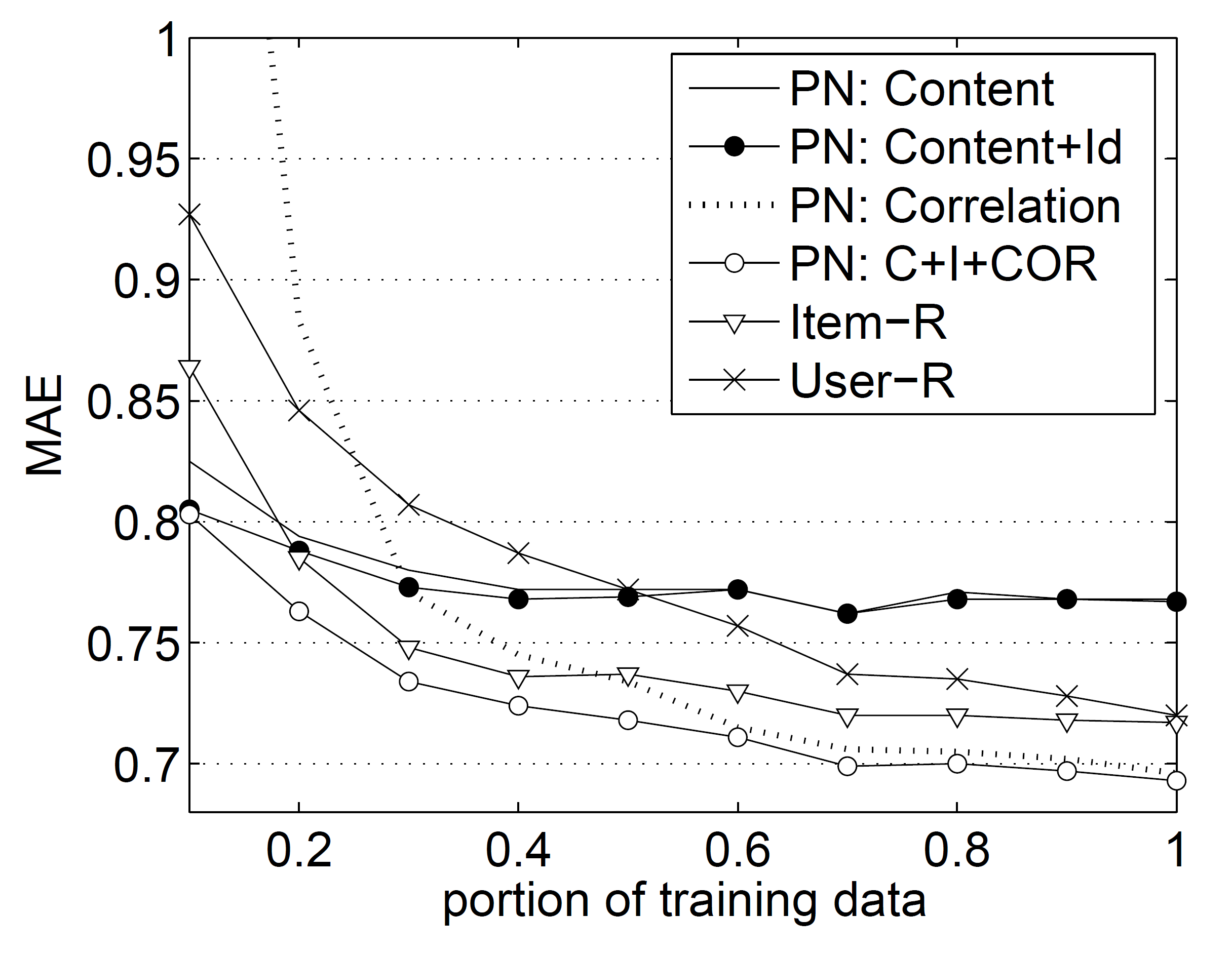
Figure 5: The mean absolute error (MAE) of recommendation methods with respect to training size of the MovieLens data. (Item: item-based method, and Item-R: item-based method with rounding, User: user-based method, User-R: user-based method with rounding, Content: PNs with content-based features, C+I+CORR: PNs with content, identity and correlation features).

Figure 6: The mean 0/1 error of recommendation methods with respect to training size of the MovieLens data. (Item: item-based method, and Item-R: item-based method with rounding, User: user-based method, User-R: user-based method with rounding, Content: PNs with content-based features, C+I+CORR: Ns with content, identity and correlation features).

4.3 Top-$N$ Recommendation

We produce a ranked list of items for each user in the test set so that these items do not appear in the training set. When a recommended item is in the test set of a user, we call it is a hit. For evaluation, we employ two measures. The first is the expected utility of the ranked list Breese et al. (1998), and the second is the MAE computed over the hits. The expected utility takes into account of the position $j$ of the hit in the list for each user $u$

$$R_{u}=\sum_{j}\frac{1}{2^{(j-1)/(\alpha-1)}}$$ (16)

where $\alpha$ is the viewing halflife. Following Breese et al. (1998), we set $\alpha=5$. Finally, the expected utility for all users in the test set is given as

$$R=100\frac{\sum_{u}R_{u}}{\sum_{u}R_{u}^{max}}$$ (17)

where $R_{u}^{max}$ is computed as

$$R_{u}^{max}=\sum_{j\in I^{\prime}(u)}\frac{1}{2^{(j-1)/(\alpha-1)}}$$ (18)

where $I^{\prime}(u)$ is the set of items of user $u$ in the test set.

For comparison, we implement a user-based recommendation in that for each user, we choose 100 best (positively) correlated users and then rank the item based on the number of times it is rated by them. Table 1 reports results of Preference Network with ranking measure of maximal energy change and expected energy change in producing the top 20 item recommendations.

Method	MAE	Expected Utility
User-based	0.669	46.61
PN (maximal energy)	0.603	47.43
PN (expected energy)	0.607	48.49

Table 1: Performance of top-20 recommendation. PN = Preference Network.

We vary the rate of recall by varying the value of $N$, i.e. the recall rate typically improves as $N$ increases. We are interested in how the expected utility and the MAE changes as a function of recall. The expected energy change is used as the ranking criteria for the Preference Network. Figure 7 shows that the utility increases as a function of recall rate and reaches a saturation level at some point. Figure 8 exhibits a similar trend. It supports the argument that when the recall rate is smaller (i.e. $N$ is small), we have more confidence on the recommendation. For both measures, it is evident that the Preference Network has an advantage over the user-based method.

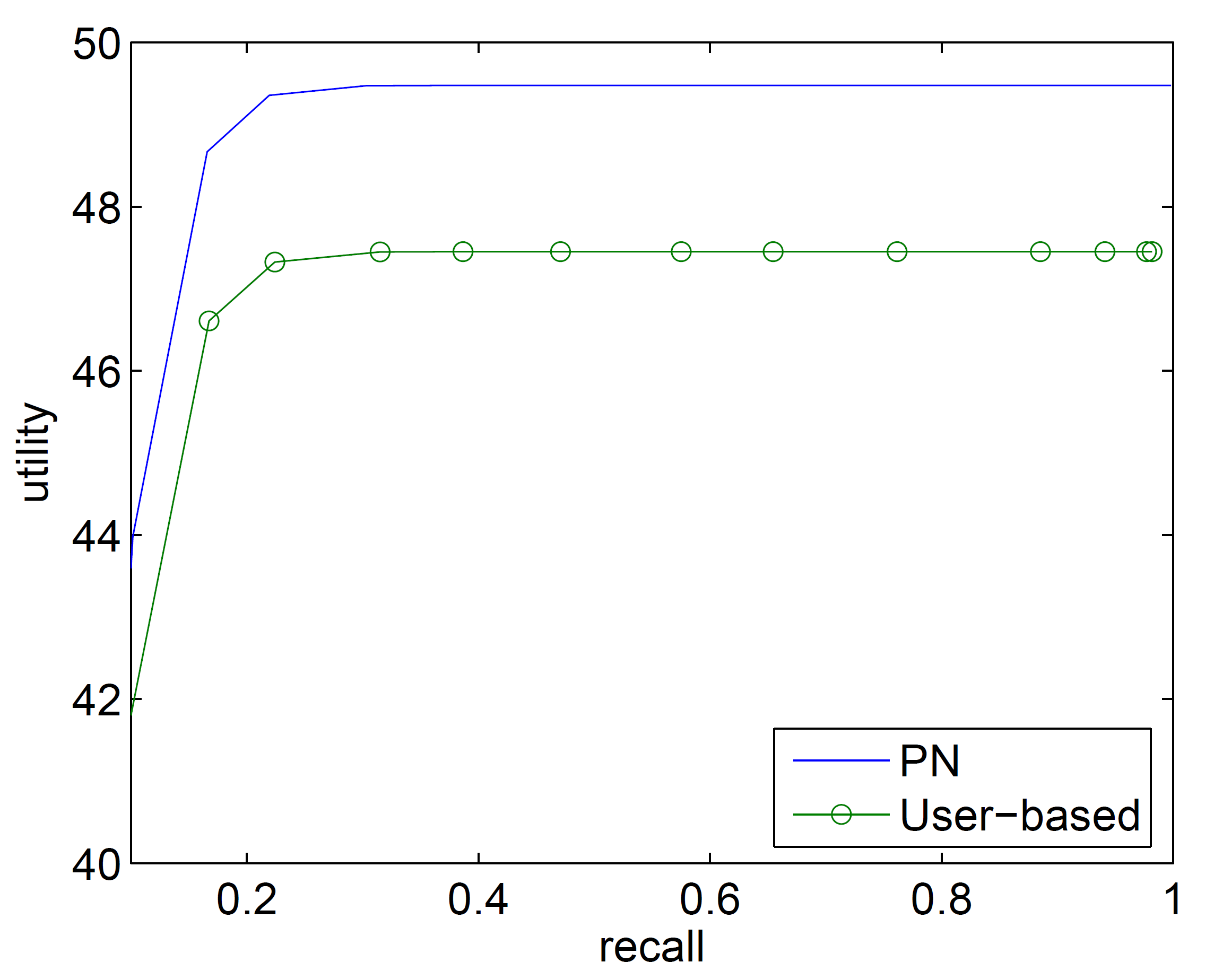
Figure 7: Expected utility as a function of recall. The larger utility, the better. PN = Preference Network.

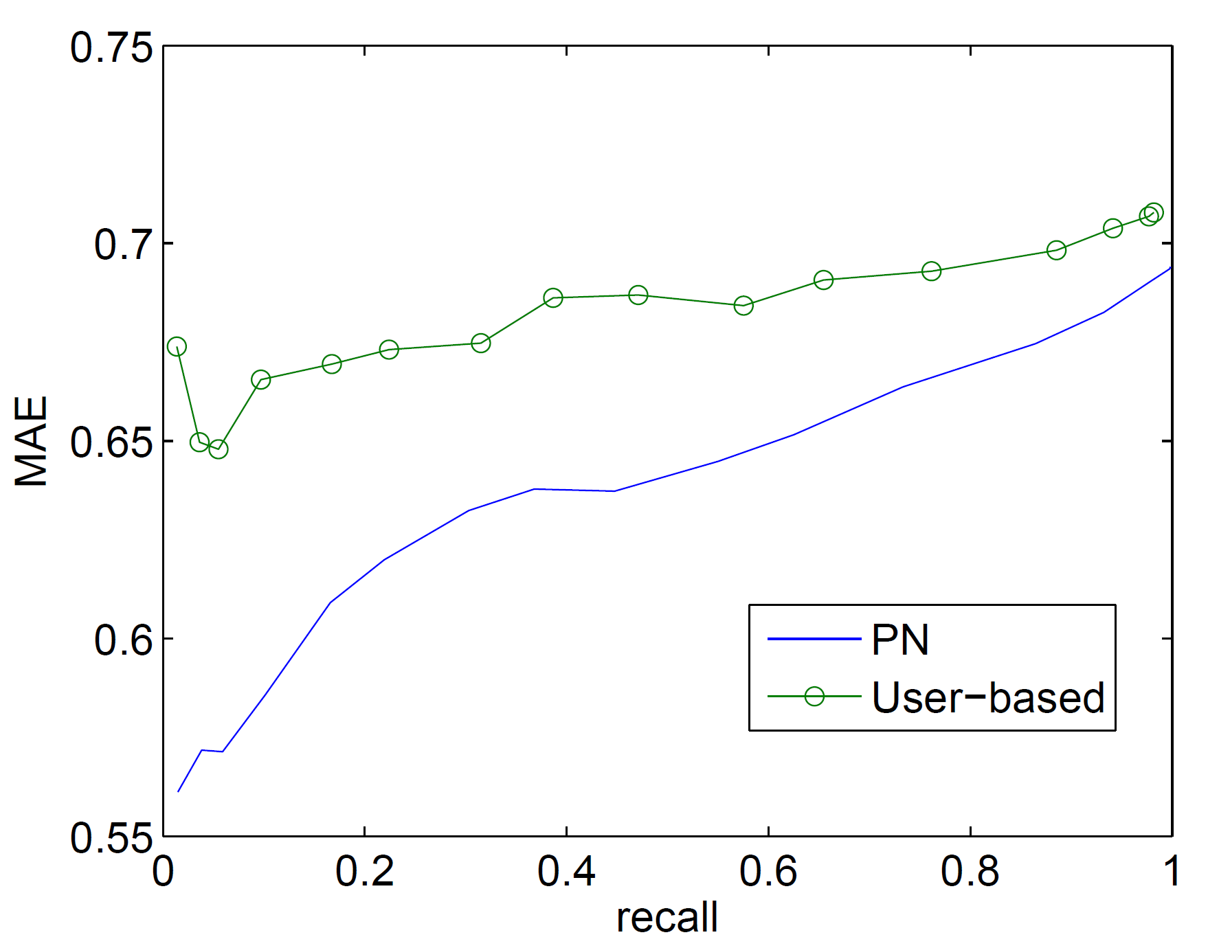
Figure 8: MAE as a function of recall. The smaller MAE, the better. PN = Preference Network.

5 Discussion and Conclusions

We have presented a novel hybrid recommendation framework called Preference Networks that integrates different sources of content (content-based filtering) and user’s preferences (collaborative filtering) into a single network, combining advantages of both approaches, whilst overcoming shortcomings of individual approaches such as the cold-start problem of the collaborative filtering. Our framework, based on the conditional Markov random fields, are formal to characterise and amenable to inference. Our experiments show that PNs are competitive against both the well-known item-based and user-based collaborative filtering methods in the rating prediction task, and against the user-based method in the top-$N$ recommendation task.

Once learned, the PN is a probabilistic database that allows interesting queries. For example, the set of most influential items for a particular demographic user group can be identified based on the corresponding energies. Moreover, the conditional nature of the PN supports fusion of varieties of information into the model through weighted feature functions. For example, the features can capture the assertion that if two people are friends, they are more likely to have similar tastes even though they have not explicitly provided any common preferences.

Finally, one main drawback the PNs inherit from the user-based methods is that it may be expensive at prediction time, because it takes into account all users who are related to the current one. On-going work will investigate clustering techniques to reduce the number of pair-wise connections between users.

Appendix A Markov Property and Learning Log-linear Models

This paper exploits an important aspect of Markov networks known as Markov property that greatly simplifies the computation. Basically, the property ensures the conditional independence of a variable $r_{t}$ with respect to other variables in the network given its neighbourhood

$$P(r_{t}|x\backslash r_{t},\mathbf{o})=P(r_{t}|\mathcal{N}(t),\mathbf{o})$$ (19)

where $\mathcal{N}(t)$ is the neighbourhood of $r_{t}$. This explains why we just need to include the neighbourhood in the Equation 7. This is important because $P(r_{t}|\mathcal{N}(t),\mathbf{o})$ can be easily evaluated

$$P(r_{t}|\mathcal{N}(t),\mathbf{o})=\frac{1}{Z_{t}}\psi_{t}(r_{t},\mathbf{o})\prod_{t^{\prime}\in\mathcal{N}(t)}\psi_{t,t^{\prime}}(r_{t},r_{t^{\prime}},\mathbf{o})$$

where $Z_{t}=\sum_{r_{t}}\psi_{t}(r_{t},\mathbf{o})\prod_{t^{\prime}\in\mathcal{N}(t)}\psi_{t,t^{\prime}}(r_{t},r_{t^{\prime}},\mathbf{o})$.

The parameter update rule in Equation 6 requires the computation of the gradient of the regularised log pseudo-likelihood in Equation 4, and thus, the gradient of the log pseudo-likelihood $L=\log P(r_{t}|\mathcal{N}(t),\mathbf{o})$. Given the log-linear parameterisation in Equations 2 and 3, we have

$$\frac{\partial\log L}{\partial{\mathbf{w}}_{v}} = {\mathbf{f}}_{v}(r_{t},\mathbf{o})-\sum_{r^{\prime}_{t}}P(r^{\prime}_{t}|\mathcal{N}(t),\mathbf{o}){\mathbf{f}}_{v}(r^{\prime}_{t},\mathbf{o})$$

$$\frac{\partial\log L}{\partial{\mathbf{w}}_{e}} = {\mathbf{f}}_{e}(r_{t},r^{\prime}_{t},\mathbf{o})-\sum_{r^{\prime}_{t}}P(r^{\prime}_{t}|\mathcal{N}(t),\mathbf{o}){\mathbf{f}}_{e}(r^{\prime}_{t},r_{t^{\prime}},\mathbf{o})$$

References

- (1)
- Adomavicius and Tuzhilin (2005) Adomavicius, G. and Tuzhilin, A. (2005), ‘Toward the next generation of recommender systems: a survey of the state-of-the-art and possible extensions’, Knowledge and Data Engineering, IEEE Transactions on 17(6), 734–749.
- Balabanović and Shoham (1997) Balabanović, M. and Shoham, Y. (1997), ‘Fab: content-based, collaborative recommendation’, Communications of the ACM 40(3), 66–72.
- Basilico and Hofmann (2004) Basilico, J. and Hofmann, T. (2004), ‘Unifying collaborative and content-based filtering’, Proceedings of the twenty-first international conference on Machine learning .
- Basu et al. (1998) Basu, C., Hirsh, H. and Cohen, W. (1998), ‘Recommendation as classification: Using social and content-based information in recommendation’, Proceedings of the Fifteenth National Conference on Artificial Intelligence .
- Besag (1974) Besag, J. (1974), ‘Spatial interaction and the statistical analysis of lattice systems (with discussions)’, Journal of the Royal Statistical Society Series B 36, 192–236.
- Billsus and Pazzani (1998) Billsus, D. and Pazzani, M. (1998), ‘Learning collaborative information filters’, Proceedings of the Fifteenth International Conference on Machine Learning pp. 46–54.
- Breese et al. (1998) Breese, J., Heckerman, D., Kadie, C. et al. (1998), ‘Empirical analysis of predictive algorithms for collaborative filtering’, Proceedings of the Fourteenth Conference on Uncertainty in Artificial Intelligence 461.
- Claypool et al. (1999) Claypool, M., Gokhale, A., Miranda, T., Murnikov, P., Netes, D. and Sartin, M. (1999), ‘Combining content-based and collaborative filters in an online newspaper’, ACM SIGIR Workshop on Recommender Systems .
- Deshpande and Karypis (2004) Deshpande, M. and Karypis, G. (2004), ‘Item-based top-N recommendation algorithms’, ACM Transactions on Information Systems (TOIS) 22(1), 143–177.
- Heckerman et al. (2001) Heckerman, D., Chickering, D., Meek, C., Rounthwaite, R. and Kadie, C. (2001), ‘Dependency networks for inference, collaborative filtering, and data visualization’, The Journal of Machine Learning Research 1, 49–75.
- Hofmann (2004) Hofmann, T. (2004), ‘Latent semantic models for collaborative filtering’, ACM Transactions on Information Systems (TOIS) 22(1), 89–115.
- Lafferty et al. (2001) Lafferty, J., McCallum, A. and Pereira, F. (2001), Conditional Random Fields: Probabilistic Models for Segmenting and Labeling Sequence Data, in ‘ICML’, pp. 282–289.
- Marlin (2004) Marlin, B. (2004), ‘Modeling user rating profiles for collaborative filtering’, Advances in Neural Information Processing Systems 16, 627–634.
- Mooney and Roy (2000) Mooney, R. and Roy, L. (2000), ‘Content-based book recommending using learning for text categorization’, Proceedings of the fifth ACM conference on Digital libraries pp. 195–204.
- Pazzani (1999) Pazzani, M. (1999), ‘A Framework for Collaborative, Content-Based and Demographic Filtering’, Artificial Intelligence Review 13(5), 393–408.
- Pearl (1988) Pearl, J. (1988), Probabilistic reasoning in intelligent systems: networks of plausible inference, Morgan Kaufmann, San Francisco, CA.
- Resnick et al. (1994) Resnick, P., Iacovou, N., Suchak, M., Bergstorm, P. and Riedl, J. (1994), GroupLens: An Open Architecture for Collaborative Filtering of Netnews, in ‘Proceedings of ACM 1994 Conference on Computer Supported Cooperative Work’, ACM, Chapel Hill, North Carolina, pp. 175–186.
- Salakhutdinov et al. (2007) Salakhutdinov, R., Mnih, A. and Hinton, G. (2007), Restricted Boltzmann machines for collaborative filtering, in ‘ICML’.
- Sarwar et al. (2001) Sarwar, B., Karypis, G., Konstan, J. and Reidl, J. (2001), ‘Item-based collaborative filtering recommendation algorithms’, Proceedings of the 10th international conference on World Wide Web pp. 285–295.
- Schein et al. (2002) Schein, A., Popescul, A., Ungar, L. and Pennock, D. (2002), ‘Methods and metrics for cold-start recommendations’, Proceedings of the 25th annual international ACM SIGIR conference on Research and development in information retrieval pp. 253–260.
- Zhang and Iyengar (2002) Zhang, T. and Iyengar, V. (2002), ‘Recommender systems using linear classifiers’, Journal of Machine Learning Research 2(3), 313–334.
- Zitnick and Kanade (2004) Zitnick, C. and Kanade, T. (2004), ‘Maximum entropy for collaborative filtering’, Proceedings of the 20th conference on Uncertainty in artificial intelligence pp. 636–643.