Imaging survey of subsystems in secondary components to nearby southern dwarfs

Abstract

To improve the statistics of hierarchical multiplicity, secondary components of wide nearby binaries with solar-type primaries were surveyed at the SOAR telescope for evaluating the frequency of subsystems. Images of 17 faint secondaries were obtained with the SOAR Adaptive Module that improved the seeing; one new 0$\farcs$2 binary was detected. For all targets, photometry in the $g^{\prime},i^{\prime},z^{\prime}$ bands is given. Another 46 secondaries were observed by speckle interferometry, resolving 7 close subsystems. Adding literature data, the binarity of 95 secondary components is evaluated. We found that the detection-corrected frequency of secondary subsystems with periods in the well-surveyed range from $10^{3}$ to $10^{5}$ days is 0.21$\pm$0.06 – same as the normal frequency of such binaries among solar-type stars, 0.18. This indicates that wide binaries are unlikely to be produced by dynamical evolution of $N$-body systems, but are rather formed by fragmentation.

1. Introduction

This paper complements multiplicity statistics in the solar neighborhood. Recently, multiplicity data on the F- and G-dwarfs within 67 pc of the Sun (the FG-67 sample) and their statistical analysis were published (Tokovinin, 2014a, b, hereafter FG67a and FG67b). This work revealed that the census of subsystems in the secondary components of nearby wide binaries is much less complete than for the main (primary) targets. To address this problem, a large survey of 212 secondary components on the northern sky has been undertaken with the Robo-AO instrument at Palomar (Riddle et al., 2014). On the southern sky, however, only a limited one-night survey of wide binaries was made with the NICI instrument (Tokovinin et al., 2010b) and a few secondaries were addressed individually by various authors.

Here we imaged 17 faint secondary components at the 4.1-m SOAR telescope using the laser-assisted adaptive optics (AO) system SAM (SOAR Adaptive Module) (Tokovinin et al., 2010c, 2012) to improve spatial resolution with respect to the seeing. Although the achieved resolution of about 0$\farcs$5 is inferior to the 0$\farcs$1 resolution of the Robo-AO, the wide corrected field of SAM allows comparison of the target image with other stars and enables binary detection down to a fraction of the Full-Width at Half Maximum (FWHM) resolution (see Terziev et al., 2013). The secondaries probed with SAM are fainter than those surveyed with Robo-AO, extending the subsystem census into the low-mass regime.

In addition to the AO-assisted classical imaging, we targeted 46 brighter secondary components with the speckle camera. Here, SOAR reaches the diffraction-limited resolution of 0$\farcs$04 in the $I$ band, surpassing Robo-AO. Thus, this survey complements the Robo-AO effort in different ways, while extending it to the southern sky. Joining new observations with data from the literature, we cover here 95 secondary components and give a statistically independent assessment of the frequency of the secondary subsystems.

The fraction of subsystems in the secondary components is a sensitive probe of formation mechanisms of binary stars. Chaotic dynamics of small $N$-body systems leads to preferential ejection of low-mass stars. Some ejected stars remain bound to their massive primaries, but they tend to be single and their wide orbits have high eccentricity (see however Fig. 3 in Reipurth & Mikkola, 2012). The alternative formation mechanism of multiple stars through fragmentation of rotating cores predicts that components on distant orbits inherit a large fraction of the total angular momentum of the core. Therefore their orbits should have moderate eccentricities, they never come very close to the main star, and no dynamical interplay takes place. In such case, the secondary components are as likely to contain subsystems as the primaries. This conclusion emerges from the study of the FG-67 sample; it is strengthened here by the new data.

In Section 2 we present observations of faint secondaries with SAM. The results of the speckle survey are given in Section 3. The complete sample of secondaries is given in Section 4, its statistical analysis is described in Section 5. Section 6 discusses the results.

2. Observations with SAM

2.1. Observing procedure

The night of March 4, 2014 was allocated for the survey with SAM through NOAO (proposal 2014A-0039). We selected from the FG-67 sample physical secondary components fainter than $V=15$ mag with separations larger than 20″  and no prior high-resolution data.

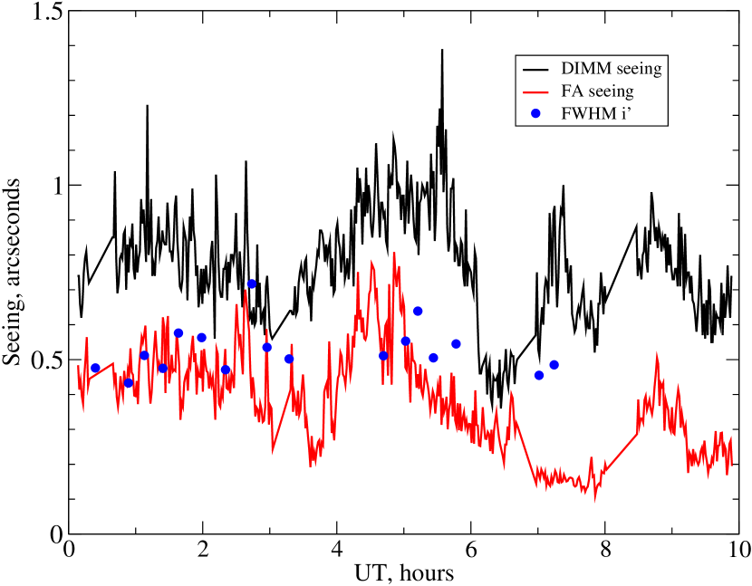
Figure 1.— Observing conditions on March 4/5, 2014. The black and red lines show the total seeing and the free-atmosphere seeing as measured, respectively, by the DIMM and MASS channels of the site monitor at Cerro Pachón. The dots show FWHM resolution of the images in closed loop in the SDSS $i^{\prime}$ filter.

The observing conditions on March 4/5, 2014 were typical for the Cerro Pachón site (Figure 1). The seeing fluctuated around its median value of 0$\farcs$7, while the seeing in the free atmosphere (produced by turbulence above 0.5 km) was mostly below 0$\farcs$5 (its median at Cerro Pachón is 0$\farcs$40, Tokovinin & Travouillon, 2008). There were light cirrus clouds at the beginning of the night which however did not prevent laser operation. The observations had to be stopped at UT 7:30 when the laser projection optics was damaged by a burned insect. In the following runs we installed a protective mesh in the laser launch telescope to prevent such incidents, without adverse effect on the SAM performance. A total of 21 targets (17 of those for this program) were pointed, with a median overhead time (from the start of the telescope slew to closing all loops) of 7 min. The SAM operated thus quite efficiently. It delivered a FWHM resolution limited mostly by the free-atmosphere seeing (Figure 1).

2.2. Data reduction

The images were acquired by the CCD of 4096$\times$4112 pixels binned 2$\times$2 to the effective pixel scale of 91 mas. It covers a square field of 186″. For each target, three images in the SDSS filters $g^{\prime}$, $i^{\prime}$, and $z^{\prime}$ (Fukugita et al., 1996) were taken with exposure times ranging from 10 s to 1 min. The data were processed in a standard way (bias subtraction and division by sky flats) using the pipeline PyRAF script of L. Fraga. Then three images in each filter were median-combined.

Figure 2 illustrates typical data. The wide binary HIP 50895AB with a separation of 42$\farcs$4 was identified by Tokovinin & Lépine (2012). The components share common proper motion and the colors of B match a dwarf of 0.2 solar mass located at the same distance as A, 54 pc. The $V$ magnitudes of A and B are 8.12 and 16.3, respectively, so the image of A is heavily saturated. The sky is not crowded, but several field stars are still available as point spread function (PSF) reference. For each secondary component, we selected at least two reference stars.

Figure 2.— Example of the SAM data and their processing. The image of HIP 50895 in the $i^{\prime}$ filter, in negative logarithmic intensity scale (North up, East to the right) is shown. The binary components A (heavily saturated) and B are marked, as well as the two reference stars (1) and (2). The lower-left insert shows the enlarged image of the component B (also in logarithmic intensity scale), the lower-right insert shows the residuals after subtracting the reference star (1) from the image of B (sub-frame of 21 pixels size, linear gray scale from $-0.04$ to $+0.073$ of the PSF maximum).

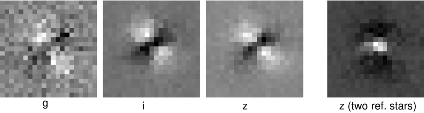
Figure 3.— Detection of the close binary HIP 53172 Ba,Bb. The images display residuals from fitting the target with the reference star (1) in three bands. The last image shows residuals from fitting reference star (1) with reference star (2).

2.3. Detection of binary companions

We developed several tools to detect and characterize potential subsystems (custom software in IDL). First, all targets and reference stars were fitted by the Moffat function. The FWHM resolution was determined from these fits, while residuals show any asymmetry of the PSF. The PSFs have a very faint “tail” on their lower-right side related to the deformable mirror in SAM. Otherwise, the PSFs are very symmetric, with ellipticity well under 0.1. The peak intensity and total flux were determined for all targets and reference stars in all three filters.

Each target was fitted by a scaled and shifted image of the reference star. This is the most sensitive test for binary companions. The fits were repeated with the second reference star, and the two reference stars were mutually cross-checked as well. We restricted the fits to the 10-pixel radius, looking for close companions (wider companions are evident anyway). The quality of the fit could be evaluated by the normalized $\chi^{2}$ metric if the residuals were dominated by the readout and shot noise. However, the major contribution to the residuals comes from slight differences between the PSFs, so the adequate metric of the fit quality is the rms residual difference normalized by the intensity. If $A_{i}$ and $B_{i}$ are intensities of the target and fitted PSF, respectively, in the subset of ${i}$ pixels, the fit quality metric $r$ is

$$r^{2}=\sum_{i}(A_{i}-B_{i})^{2}/\sum_{i}A_{i}^{2}.$$ (1)

The median value of $r$ in all filters is about 0.05, and it does not exceed 0.1. The lower-right insert in Figure 2 shows the residual pattern with $r=0.047$: a bright central zone and a dark halo. The AO correction was slightly better for the target star than for the reference (1) (FWHMs of 0$\farcs$72 and 0$\farcs$75, respectively), causing the residual mismatch. A similar pattern is seen when the target is fitted by the reference (2), $r=0.051$. On the other hand, the two reference stars (1) and (2) are located close to each other and match better, $r=0.021$.

Among the 17 observed targets, we detected only one new subsystem in HIP 53172B. This is a late-M dwarf with estimated mass of $0.1{\cal M}_{\odot}$ located at 279″  from the main component A (Tokovinin & Lépine, 2012). Its distance from the Sun is 47 pc, $V$-magnitudes of A and B are 7.76 and 19.8, respectively (A was outside the SAM field). The residuals to the PSF fits in all filters consistently show a “butterfly” pattern expected for an equal-component binary (Figure 3), while the two reference stars match each other better. The same asymmetry is seen when approximating the target by a Moffat function. This detection is not absolutely certain, but very likely.

The parameters of the binary pair HIP 53172 Ba,Bb were determined by a procedure similar to the PSF fit. Instead of adjusting only relative position and intensity ratio to the PSF star, the fitting routine now assumes that the target is a binary and adjusts three additional parameters (relative position of the binary components and their intensity ratio). In the case of HIP 53172 Ba,Bb, we found the separation of $\sim$2 pixels (0$\farcs$18) at a position angle of $\sim 320^{\circ}$, with equal intensity ($\Delta m=0$). Consistent binary parameters are found in all three filters and while using either of the two reference stars. The FWHM resolution is 0$\farcs$5 in both $i^{\prime}$ and $z^{\prime}$ filters. So, the binary separation is less than half of the FWHM, its measurement is quite uncertain and cannot be used in the future orbit calculation (the estimated orbital period is a few decades). The quality of the PSF fits in the $z^{\prime}$ filter using reference stars (1) and (2) is 0.063 and 0.095, respectively. By fitting the double-star model, the residuals improve to 0.033 and 0.027. Similar improvement of residuals is found in the $i^{\prime}$ filter when fitting a double star instead of the PSF.

Figure 4.— Sensitivity of the rms residual $r$ from the PSF fit (on vertical axis) to binary separation. The target HIP 43279B was used to simulate binaries with equal components and fit them by the reference star (1). The legend gives the FWHM resolution.

To determine the sensitivity to subsystems, we simulated binaries and fitted them by reference stars. By adopting a conservative detection threshold of $r>0.1$, we found that an equal-magnitude binarity is securely detected at a separation equal to half of the FWHM resolution (Figure 4), while at a separation equal to the FWHM the detectable intensity ratio is about 0.16, or $\Delta m<1.8$. We further adopt $\Delta m<3.2$ at 0$\farcs$7 and $\Delta m<5$ at 5″, independently of the FWHM. The deepest detection in terms of the mass ratio is in the band $z^{\prime}$, where the FWHM resolution is better and the low-mass companions are brighter. These detection limits are adopted in the statistical analysis presented below. They are obviously approximate and conservative (the new pair HIP 53172 Ba,Bb is just below the limit). To verify the absence of other detectable close companions, we ran the binary-fitting algorithm on all targets. It returned “binaries” with separations of less than 2 pixels. There was no agreement between binary parameters in different filters, while the residuals from fitting double stars were not substantially reduced in comparison to the PSF fits.

2.4. Photometry

For each field, we determined instrumental magnitudes of stars detected in all three filters by aperture photometry with the aperture radius of 10 pixels and the sky radius of 20 pixels. The zero point of the instrumental magnitudes corresponds to 25 mag for a flux of 1 count per second.

Four targets in the equatorial zone covered by the SDSS (HIP 43172, 43297, 56738, 60081) were used for photometric calibration. Stars in these fields were matched to the SDSS Data Release 9 (Ahn et al., 2012) using the TOPCAT tool. We calibrate instrumental magnitudes against the PSF magnitudes of SDSS. After rejecting a few outliers and stars fainter than $g^{\prime}=19$, we got 22 matches and fitted the instrumental magnitudes by linear relations like

$$g^{\prime}_{\rm inst}=g^{\prime}_{\rm SDSS}+a+b\;(g^{\prime}-i^{\prime})_{\rm SDSS}.$$ (2)

The $(g^{\prime}-i^{\prime})_{\rm SDSS}$ color term is used for all filters. The extinction was not considered explicitly, being included in the zero-points $a$, because the range of air mass was small (from 1.04 to 1.27) and we did not measure the extinction. Table 1 gives the zero points and color terms (of which the only significant one is in $i^{\prime}$) and the rms residuals to those linear fits. The linear equations were inverted to translate instrumental magnitudes into the standard SDSS system. Photometry is not the main goal of our program, just a by-product, and its accuracy is about $\pm$0.05 mag.

Table 1Reduction to the SDSS photometric system

Filter	$a$	$b$	rms
$g^{\prime}$	$-0.609\pm 0.025$	$0.008\pm 0.018$	0.066
$i^{\prime}$	$-0.292\pm 0.013$	$-0.054\pm 0.08$	0.029
$z^{\prime}$	$0.172\pm 0.019$	$0.009\pm 0.014$	0.052

Table 2Photometry of secondary components with SAM

Name	$g^{\prime}$	$i^{\prime}$	$z^{\prime}$	Air	FWHM
	(mag)	(mag)	(mag)	mass	(arcsec)
28267D	16.90	13.58	12.76	1.12	0.58
32650C	17.33	14.39	13.76	1.27	0.41
41211B	16.96	13.73	12.92	1.15	0.47
41211C	18.08	14.32	13.22	1.17	0.40
43172D	18.98	15.64	14.72	1.20	0.50
	18.91	15.62	14.70
43297B	15.93	13.00	12.16	1.23	0.42
	16.00	16.03?	12.21
49520C	17.74	14.83	14.09	1.11	0.52
50895B	17.04	14.18	13.46	1.13	0.66
53172B	18.88	15.62	14.77	1.13	0.54
54530B	17.62	17.09	17.17	1.09	0.44
55455B	16.72	13.62	12.90	1.26	0.59
56738B	17.03	13.79	12.92	1.15	0.42
	17.04	13.84	12.90
57443B	13.87	10.87	10.08	1.04	0.53
60081B	17.69	17.13	17.36	1.15	0.47
	17.69	17.29	17.37
60620C	16.63	13.97	13.29	1.06	0.47
64056B	16.29	13.59	12.91	1.04	0.42
66530B	15.71	13.03	12.39	1.01	0.43

Note. — The SDSS-DR9 photometry is given in italics.

Table 2 lists 17 secondary components observed with SAM (their equatorial coordinates are given in Table 3), their measured SDSS magnitudes $g^{\prime}$, $i^{\prime}$, and $z^{\prime}$, the air mass, and the FWHM resolution in the $z^{\prime}$ band. The SDSS magnitudes available for the 4 targets in common with this work are given in Table 3 in italics; they agree well, except the $i^{\prime}$ magnitude of HIP 43279B which appears to be corrupted in the SDSS. On the other hand, the $V$ magnitudes estimated from $g^{\prime}$ as $V_{g}=g^{\prime}+0.297-0.366(g^{\prime}-Ks)+0.025(g^{\prime}-Ks)^{2}$ differ substantially from the $V$ magnitudes listed in FG67a; the listed magnitudes are based on the photographic photometry of (Tokovinin & Lépine, 2012). For the resolved binary HIP 53172, we estimate $V_{g}=17.86$ instead of 19.8 quoted above.

Figure 5.— Color-magnitude diagram of secondary components (squares) in the SDSS $g^{\prime}$ and $i^{\prime}$ bands. The full line shows polynomial relations from FG67a with wavelengths of 520 nm and 770 nm, where asterisks mark masses of 0.3, 0.2, 0.15, and 0.1 ${\cal M}_{\odot}$. The dashed line is based on the Table 3 of Covey et al. (2007), pluses mark spectral types from M3V to M6V.

Our program included two white dwarf secondaries (HIP 54530B and 60081B) which differ from the remaining stars by their “blue” colors. We did not find any close companions to those white dwarfs. The statistical analysis in Section 5 considers only the remaining 15 red-dwarf secondaries.

Figure 5 presents the color-magnitude diagram (CMD) of low-mass secondary components, constructed using the known distance to their primary components. For low-mass stars, standard relations in the SDSS colors are not well established. The dashed line is the polynomial relation from FG67a where the effective wavelengths of $g^{\prime}$ and $i^{\prime}$ are chosen to be 520 nm and 770 nm, respectively, to roughly match the data. The main sequence based on the Table 3 of Covey et al. (2007) is plotted in dashed line. The luminosity of low-mass stars depends on their metallicity (which is not measured for most primary targets) and age as well as on mass, therefore the points in Figure 5 do not align along a single sequence. Equal-mass binaries are readily detected by their position in the CMDs of open clusters (see e.g. Figure 4 of Sarro et al., 2012), but this method does not work for this field sample.

3. Speckle observations

In January–March 2014, speckle interferometry was performed at SOAR to follow the orbital motion of close and “fast” visual binaries. During five allocated nights, we occasionally pointed secondary components in wide nearby binaries to complement the work done with SAM. Although the speckle camera was mounted on SAM, the laser guide star was not used in order to maintain high efficiency (150 stars per night on average). As the secondary components are red and mostly faint, they were observed in the $I$ filter with a field of view of 3″. A total of 46 secondary components with separations larger than 3″  were pointed. These observations had a low priority, being a “filler” in the main speckle program.

The speckle camera and data reduction are described by Tokovinin et al. (2010a). The speckle data pipeline evaluates maximum detectable magnitude difference $\Delta m$ at separations of 0$\farcs$15 and 1″. At the diffraction limit (0$\farcs$042 at 770 nm), a detectable binary is assumed to have $\Delta m<0.5$. Among the 46 observed secondaries, 7 were resolved for the first time, while three more contain previously known resolved subsystems. The measurements of resolved secondary components will be published later with the rest of the binary-star measurements. Here we give only the relevant information, namely the detection limits for all observed secondary components and the separation and magnitude difference of the newly resolved subsystems. Most of the new pairs were confirmed on other dates or in the $y$ filter; some of them were already known as spectroscopic and/or acceleration binaries.

4. Combined data

For the statistical analysis, we combine the secondary components surveyed here with data from the literature. We selected from the main FG-67 database secondary components for which high-resolution imaging is available, south of $+15^{\circ}$ declination, and with separations larger than 3″  from the primary targets. The components surveyed by Robo-AO were excluded to make this analysis statistically independent. Apart from this work, the next largest data set is furnished by the mini-survey with NICI (Tokovinin et al., 2010b).

Table 3 lists the complete sample of 95 secondary components discussed here. Its first columns contain the Hipparcos number of the main FG-67 target HIP1, component identification, its separation from the main target, and the approximate equatorial coordinates in degrees as given in FG67a. Then follow the wavelength of imaging data in nm and the detection limits (4 separations and 4 values of $\Delta m$). The last column contains the reference code, explained in the notes to the table. The code SAM refers to the data of Section 2, SOAR means speckle observations (Section 3).

The data on secondary subsystems in this sample are collected in Table 4. Its first column identifies the secondary component. The second column gives the discovery method(s) (’a’ – astrometric acceleration, ’s,S’ – spectroscopic, ’v,V’ – direct resolution). For resolved subsystems, we give in the columns (3) and (4) angular separation $\rho$ and magnitude difference $\Delta m$ together with the filter to which it refers. The orbital periods and component’s masses are estimated as explained in FG67a. Comments and references are provided in the last column and in the notes to the table. Known visual pairs are identified by their “discoverer codes” given in the WDS (Mason et al., 2001). For these pairs, the WDS detection limits in Table 4 are adopted from FG67a, e.g. $\Delta m=2.5$ at 0$\farcs$15.

Table 3List of secondary components with high-resolution imaging data (fragment)

HIP1		Sep.	RA(2000)	Dec(2000)	$\lambda$	$\rho_{1}$ to $\rho_{4}$				$\Delta m_{1}$ to $\Delta m_{4}$				Ref.
		(arcsec)	(deg)	(deg)	(nm)	(arcsec)				(mag)
9902	B	52.2	31.8843	$-$59.6726	1690	0.118	0.306	1.969	6.0	0.0	3.9	7.9	7.9	Cvn2010
10579	B	6.7	34.0369	$-$21.0076	2272	0.054	0.140	0.900	9.0	0.0	3.9	7.9	7.9	NICI
14954	B	6.8	48.1925	$-$1.1977	2200	0.060	1.000	2.000	5.0	1.0	6.3	8.6	9.9	Mug2009
15371	B	309.1	49.4423	$-$62.5753	540	0.042	0.150	1.000	1.50	0.5	3.7	6.1	6.1	SOAR
20552	B	5.5	66.0483	$-$57.0720	2272	0.054	0.140	0.900	9.0	0.0	3.9	7.9	7.9	NICI
20598	B	3.2	66.1747	$-$8.7524	770	0.029	0.150	1.000	1.50	0.5	3.2	3.7	3.7	SOAR
21963	B	8.2	70.8207	$-$9.6182	2272	0.054	0.140	0.900	9.0	0.0	3.9	7.9	7.9	NICI
22611	B	99.6	72.9498	$-$34.2214	770	0.042	0.150	1.000	1.50	0.5	3.4	3.9	3.9	SOAR

Note. — Bouy2008: Bouy et al. (2008); Burg2005: Burgasser et al. (2005); Clo2003: Close et al. (2003); Cvn2010: Chauvin et al. (2010); Jay2001: Jayawardhana & Brandeker (2001); Egg2007: Eggenberger et al. (2007); MH09: Metchev & Hillenbrand (2009); Mug2009: Mugrauer & Neuhaeuser (2009); NICI: Tokovinin et al. (2010b); SAM, SOAR: this work; Tok2006: Tokovinin et al. (2006); WDS: Visual micrometer resolution.

Table 4Secondary subsystems

Name	Type	$\rho$	$\Delta m$	$\log P$	${\cal M}_{1}$	${\cal M}_{2}$	Notes
		(arcsec)	(mag)	(days)	(${\cal M}_{\odot}$)	(${\cal M}_{\odot}$)
14954B	S1,V	0.064	…	2.87	0.52	0.06	Mugrauer & Neuhaeuser (2009), false exo-planet
34065C	S1,v,a	0.227	4.4 I	3.23	0.71	0.16	SOAR, HIP 34052, Sahlmann et al. (2011): $P=4.62$ yr
35554B	S1	…	…	2.09	1.22	1.12	HD 57853, Saar et al. (1990): triple, 122 d and $\sim$10 d
36165B	s	…	…	…	0.91	…	HIP 36160. Nordström et al. (2004): RV variable
36395C	v,S1	0.090	1.2 I	3.33	0.56	0.37	SOAR, NLTT 17952 (F – unresolved)
36485D	v,S1	0.114	2.5 I	3.43	1.05	0.61	SOAR, HIP 36497, Halbwachs et al. (2012): $P=7.41$ yr
38908BC	v	2.3	3.6 V	4.96	0.60	0.21	JSP 208BC
43557B	s2	…	…	1.0?	0.37	0.37	Fuhrmann et al. (2005): double-lined
45170E	v	0.53	0	4.61	0.05	0.05	GJ 337C, Burgasser et al. (2005): L8/T brown dwarfs
45734B	s2	…	…	…	0.93	0.74	Desidera et al. (2006): double-lined
46535A	v	0.70	3.1 V	4.62	1.21	0.76	HDS 1360, B=HIP 46253 is primary
49520B	v	0.213	3.6 K	4.16	0.99	0.26	Tokovinin et al. (2010b)
53172B	v	0.18	0	4.32	0.09	0.09	SAM
59021B	S2	…	…	2.17	0.84	0.67	double-lined (D. Latham, private communication)
66676BC	v	0.918	3.7 I	5.05	0.96	0.38	SOAR
72235B	v	0.412	4.1 I	4.44	0.70	0.17	SOAR
76435C	v	0.056	0.4 I	3.15	0.70	0.66	SOAR
79980B	v	0.040	1.4 I	2.70	1.16	1.00	SOAR, HIP 79979, Nordström et al. (2004): RV variable
85342B	v,s,a	1.01	2.4 I	5.09	0.93	0.63	SOAR
101806B	v	0.42	0.79 K	4.72	0.26	0.19	Eggenberger et al. (2007), A is exo-host
113579B	v	1.84	0.55 V	5.13	0.70	0.65	RST 1154, HIP 113597
114702B	v	0.053	1.2 K	2.91	0.90	0.66	Tokovinin et al. (2006), triple
116106BC	v	0.586	2.4 K	4.78	0.10	0.03	Bouy et al. (2008)

5. Statistical analysis

The methods of statistical analysis of secondary subsystems are identical to those used for the whole FG-67 sample (see FG67b). Separation and magnitude difference $(\rho,\Delta m)$ are converted to period $P$ (assuming that the separation equals semi-major axis) and mass ratio $q$ (standard relations for main sequence translate absolute magnitudes to mass). The detection limits in $(\rho,\Delta m)$ are translated to the $(P,q)$ space with the same assumptions. In the cases when other detection techniques such as radial velocity (RV) or Hipparcos acceleration are available, they are included as well. Upper limits on the periods of potential subsystem imposed by the dynamical stability are modeled statistically, as explained in FG67b.

Figure 6.— Period and mass ratio of secondary subsystems (squares). The contours show average detection probability. The estimated fraction of dynamically stable subsystems $F_{\rm dyn}(P)$ is plotted in thick line. The upper axis corresponds to angular separation at a distance of 50 pc.

Figure 6 shows the distribution of secondary subsystems in the $(P,q)$ plane and the detection limits for our sample of secondaries. Of the 23 secondary subsystems, 21 have estimates of $P$ and $q$, the remaining two are spectroscopic binaries with yet unknown periods. Subsystems with long periods and wide separations are not expected because they would be dynamically unstable in the wide outer binaries. The thick line in Figure 6 shows the fraction of dynamically stable subsystems $F_{\rm dyn}(P)$. All secondary subsystems have periods shorter than $10^{5.1}$ d and sub-arcsecond separations (the widest pair HIP 113579B = RST 1154 would have $\rho=1\farcs 15$ at a standard distance of 50 pc). Some of the surveyed binaries are quite wide and could contain subsystems with separations of a few arcseconds. Such subsystems exist around some primary targets, but none were found around the secondaries, despite the ease of their detection. However, as noted in FG67a, there is a bias against discovery of wide secondary components that are themselves partially resolved binaries.

Subsystems with periods from $10^{3}$ to $10^{5}$ days have a good detection probability and are not strongly affected by the dynamical stability. There are 12 secondary subsystems with such periods, or a raw subsystem frequency of $12/95=0.126$. We correct for incomplete detection by assuming that the mass ratio $q$ in the secondary subsystems is distributed as $q^{\beta}$ with $\beta=0$ or $\beta=1$. These two assumptions correspond to the detection probability of 0.60 and 0.74 and lead to the detection-corrected companion frequency of $0.21\pm 0.06$ and $0.17\pm 0.05$, respectively, in the selected range of periods. The uncertainty related to the choice of $\beta$ is less than the statistical errors.

Figure 7.— Cumulative distribution of periods in the secondary subsystems (dashed line) and its model (full line).

By looking at Figure 6, we note that the mass ratios of secondary subsystems do not show concentration to $q\sim 1$ but are distributed over the whole range. Fitting the data by the log-normal period distribution and the power-law $q$-distribution using the maximum likelihood method (see FG67b) leads to $\beta=0.09\pm 0.04$ for this sample, while $\beta\sim 1$ was derived for secondary subsystems in the full FG-67 sample. So, we retain the estimate of subsystem frequency of $0.21\pm 0.06$ as the most plausible.

Binaries with solar-type primaries are described by the log-normal period distribution with a median of $10^{4.54}$ days, logarithmic dispersion of 2.40, and companion fraction of 0.56 (FG67b). The companion fraction in the selected two decades of period is then 0.18, matching within errors the fraction of secondary subsystems found here.

We tried to evaluate whether the absence of relatively wide secondary subsystems is significant. The statistical model of independent multiplicity developed in FG67b describes the period distribution of subsystems by a product of the log-normal generating period distribution and the dynamical constraint $F_{\rm dyn}(P)$ imposed by the outer binaries. The full line in Figure 7 depicts this model for the sample of secondaries studied here. It predicts that about a quarter of secondary subsystems (5 out of 23) should have separations above 1 arcsec. The cumulative histogram of the actual secondary periods is plotted in dashed line. It is not corrected for the observational selection (e.g. detection probability $<0.3$ at $P<10^{3}$ d, see Figure 6). Addition of short undetected periods would move the dashed line further to the left. The emerging tentative conclusion is that the periods of secondary subsystems are indeed shorter than predicted by the dynamical stability constraint alone.

6. Discussion

This study confirms that the occurrence of subsystems in the secondary components of wide binaries is as likely as the binarity of their main solar-type primaries.

With SAM, we probed binarity of 15 very low mass (VLM) secondaries. Their median mass is only 0.16 ${\cal M}_{\odot}$, the most massive (HIP 64056B) has a mass of 0.28 ${\cal M}_{\odot}$ and the smallest (HIP 41211C) is only 0.11 ${\cal M}_{\odot}$. The new pair HIP 53172 Ba,Bb has components of 0.10 ${\cal M}_{\odot}$. One detected binary out of 15 means a 0.07 fraction of subsystems, which is less than $23/95=0.24$ for the whole sample. However, the resolution of SAM is inferior in comparison to speckle interferometry and full AO, so a lower detection rate is expected. VLM binaries tend to be closer than 15 AU, with a peak separation around 5 AU (Close et al., 2003). This translates to angular separations of 0$\farcs$3 and 0$\farcs$1, respectively, at 50 pc distance. Most VLM binaries within 67 pc are too close to be resolved by SAM. If low-mass components of wide binaries are similar to other VLM stars, the detection of just one subsystem here is normal.

The binarity of VLM stars is better studied at diffraction-limited resolution using large telescopes, AO, and infrared detectors. Among the 23 secondary subsystems in Table 4, two (HIP 45170 Ea,Eb and HIP 116106 BC) are such VLM pairs discovered by adequate techniques. Although another VLM binary was found here with SAM, we could not measure accurately its relative position.

On the other hand, bright secondary components of larger mass can be effectively surveyed by speckle interferometry which does reach the diffraction-limited resolution. Seven new pairs (one of them actually triple) are added by this work. Many secondaries are bright enough for RV monitoring. It is obvious from Figure 6 that the census of secondary subsystems is very poor at short periods, so their RV survey is needed.

The fraction of secondary subsystems with $x=\log P$ from 3 to 5 is found here to be $0.21\pm 0.06$ or $0.17\pm 0.05$, depending on the assumption about the mass-ratio distribution. Adopting $\beta=1$, Riddle et al. (2014) found the detection-corrected frequency of $0.13\pm 0.03$ in a smaller period range from 3.5 to 5; this translates to $0.17\pm 0.04$ when scaled to the 2-dex period interval. The two independent samples of wide secondary components studied by different instruments gave the same result, enhancing its confidence.

Riddle et al. (2014) found that the presence of secondary and primary subsystems is correlated. The southern sample of 95 secondaries studied here contains 36 primary subsystems, 8 of which also have secondary subsystems (i.e. are 2+2 quadruples). If the occurrence and discovery of primary and secondary subsystems are mutually independent, the expected number of coincidences is $95\times(23/95)\times(36/95)=8.7$. Therefore, this smaller sample shows no evidence of the correlation discovered by Riddle et al. (2014) and confirmed in FG67b.

By gathering data on hierarchical multiple systems, we advance the understanding of their origin. To first order, hierarchical multiples can be described by picking randomly inner and outer subsystems from the same generating distribution of periods and keeping only stable configurations. However, the reality deviates from this simplistic model of independent multiplicity in several ways. Here we noted the lack of relatively wide secondary subsystems (if present, they would have been readily detected).

Close et al. (2003) believe that short periods of VLM binaries cannot be explained by their ejection from young clusters. Similarly, the secondary subsystems are closer than allowed by the outer binaries, meaning that the dynamics alone is not a valid explanation for their short periods. Rather, this feature could be related to the correlation between mass and angular momentum in the epoch of mass accretion when the properties of nascent binaries and multiples are established.

References

- Ahn et al. (2012) Ahn, C. P., Alexandroff, R., Allende Prieto, C. et al. 2012, ApJS, 203, 21 (see http://www.sdss3.org/dr9/)
- Bouy et al. (2008) Bouy, H., Martín, E. L., Brandner, W. et al. 2008, A&A, 481, 757
- Burgasser et al. (2005) Burgasser, A. J., Kirkpatrick, J. D. & Lowrance, P. J. 2005, AJ, 129, 2849
- Chauvin et al. (2010) Chauvin, G., Lagrange, A.-M., Bonavita, M. et al. 2010, A&A, 509, 52
- Close et al. (2003) Close, L. M., Siegler, N., Freed, M., & Biller, B. 2003, ApJ, 587, 407
- Covey et al. (2007) Covey, K. R., Ivezić, Z., Schlegel, D. et al. 2007, AJ, 134, 2398
- Desidera et al. (2006) Desidera, S., Gratton, R. G., Lucatello, S. et al. 2006, A&A, 454, 553
- Eggenberger et al. (2007) Eggenberger, A., Udry, S., Chauvin, G. et al. 2007, A&A, 474, 273
- Fuhrmann et al. (2005) Fuhrmann, K., Guenther, E., König, B. & Bernkopf, J. 2005, MNRAS, 361, 803
- Fukugita et al. (1996) Fukugita, M., Ichikawa, T., Gunn, J. E. et al. 1996, AJ, 111, 1748
- Halbwachs et al. (2012) Halbwachs, J.-L., Mayor, M., & Udry, S. 2012, MNRAS, 422, 14
- Jayawardhana & Brandeker (2001) Jayawardhana, R. & Brandeker, A. 2001, ApJ, 561, L111
- Mason et al. (2001) Mason, B. D., Wycoff, G. L., Hartkopf, W. I., Douglass, G. G. & Worley, C. E. 2001, AJ, 122, 3466
- Metchev & Hillenbrand (2009) Metchev, S. A. & Hillenbrand, L. A. 2009, ApJS, 181, 62
- Mugrauer & Neuhaeuser (2009) Mugrauer, M. & Neuhaeuser, R. 2009, A&A, 494, 373
- Nordström et al. (2004) Nordström, B., Mayor, M., Andersen, J. et al. 2004, A&A, 418, 989
- Reipurth & Mikkola (2012) Reipurth, Bo & Mikkola, S. 2012, Nature, 492, 221
- Riddle et al. (2014) Riddle, R., Tokovinin, A., Mason, D. B. et al, 2014, ApJ, in preparation.
- Saar et al. (1990) Saar, S. H., Nordström, B., & Andersen, J. 1990, A&A, 235, 291
- Sahlmann et al. (2011) Sahlmann, J. Ségransan, D., Queloz, D. et al. 2011, A&A, 525, 91
- Sarro et al. (2012) Sarro, L. M., Bouy, H., Berihuete, A. et al. 2012, A&A, 563, 45
- Terziev et al. (2013) Terziev, E., Law, N. M., Arcavi, I. et al. 2013, ApJS, 206, 18
- Tokovinin et al. (2006) Tokovinin A., Thomas S., Sterzik M., & Udry S. 2006, A&A, 450, 681
- Tokovinin & Travouillon (2008) Tokovinin, A. & Travouillon, T. 2008, MNRAS, 365, 1235
- Tokovinin et al. (2010a) Tokovinin, A., Mason, B., & Hartkopf, W. 2010a, AJ, 139, 743
- Tokovinin et al. (2010b) Tokovinin, A., Hartung, M., & Hayward, Th. L. 2010b, AJ, 140, 510
- Tokovinin et al. (2010c) Tokovinin, A., Tighe, R., Schurter, P., et al. 2010c, Proc. SPIE, 7736, 132
- Tokovinin et al. (2012) Tokovinin, A., Tighe, R., Schurter, P., et al. 2012, Proc. SPIE, 8447, 166
- Tokovinin & Lépine (2012) Tokovinin, A. & Lépine, S. 2012, AJ, 144, 102
- Tokovinin (2014a) Tokovinin, A. 2014a, AJ, 147, 86 (FG67a)
- Tokovinin (2014b) Tokovinin, A. 2014b, AJ, 147, 87 (FG67b)