Dependence of fluid flows in an evaporating sessile droplet on the characteristics of the substrate

Abstract

Temperature distributions and the corresponding vortex structures in an evaporating sessile droplet are obtained by performing detailed numerical calculations. A Marangoni convection induced by thermal conduction in the drop and the substrate is demonstrated to be able to result not only in a single vortex, but also in two or three vortices, depending on the ratio of substrate to fluid thermal conductivities, on the substrate thickness and the contact angle. The “phase diagrams” containing information on the number, orientation and spatial location of the vortices for quasistationary fluid flows are presented and analysed. The results obtained demonstrate that the fluid flow structure in evaporating droplets can be influenced in a controlled manner by selecting substrates with appropriate properties.

I Introduction

It is known that the evaporating flux density along the surface of a drying sessile droplet is inhomogeneous and diverges on approach to the pinned contact line Deegan97 ; Deegan2000 . The evaporation can induce temperature variations in the vicinity of the substrate–liquid interface and along the drop surface. A temperature variation along the liquid–vapor interface can in turn generate a thermocapillary flow inside the drop which has been intensively studied (see, for example, the review articles Erbil ; Larson and references therein). Sessile drop evaporation processes and structures of the fluid flow are of interest for important applications in ink-jet printing Park2006 ; Calvert2001 , spraying of pesticides Zhu2009 , micro/nano fabrication Xia2008 ; Caroll2006 , thin film coatings Kimura2003 , biochemical assays Nguyen2002 , spray cooling Jia2003 , disease diagnosis Brutin2011 ; Trantum2012 , deposition of DNA/RNA micro-arrays Schena1995 ; Fang2006 ; McHale2007 , and manufacture of novel optical and electronic materials Kawase2001 .

The substrate temperature distribution under the drop can be measured using thermo-chromic liquid crystals Sodtke2007 and with IR thermography Tarozzi2007 . The substrate properties play an important role in the nanotechnology applications of the problem. One of the examples is self-assembly of superlattices of nanoparticles taking place during evaporation of colloidal solutions. It is known that substrate characteristics can strongly influence both the deposition patterns and the self-assembly process Voylov ; Wang ; Ge ; Cai ; Lin2 ; Bigioni .

Numerical calculations of Marangoni convection in an axially symmetrical evaporating droplet agree well with corresponding experimental data HuLarsonReverse ; SavinoFico . A sensitivity of Marangoni fluid flows to the droplet contact angle is known since Hu and Larson demonstrated that fluid circulation in the vortex can reverse its sign at a critical contact angle for a drop placed onto substrates with finite thicknesses HuLarsonMarangoni . It was originally observed and described by Ristenpart et al. that the circulation direction depends on the substrate to liquid ratio of the thermal conductivities Ristenpart . Specifically, the authors found that the ratio determines the sign of the tangential component of the temperature gradient at the surface close to the contact line, and, therefore, it determines a direction of the circulation in that region. Assuming the key role of a small vicinity of the contact line in forming the circulation direction in a single vortex, the shape of the liquid–vapor interface in that small region was approximated as a plane, which is actually inappropriate since the three-phase contact line has finite radius of curvature. However, the conditions for the circulation sign change have been found within such framework. While the approach and predictions of Ref. Ristenpart generally are qualitatively insightful and quite useful, the particular approximations made and the corresponding quantitative results obtained in Ristenpart have not been justified by more accurate numerical calculations. For example, it follows from the analytical results of Ristenpart that for $k_{R}<1.45$ and $k_{R}>2$ the circulation direction is insensitive to the contact angle. The results of more recent numerical calculations, as well as the results of the present study, do not confirm this statement.

An alternative approach suggested by Xu et al. Xu , focuses on a heat transfer in the immediate vicinity of the symmetry axis piercing the apex. The change of sign of the tangential gradient of the temperature near the apex and, hence, the corresponding transition between the opposite circulation directions, taking place with a variation of the relative substrate–liquid thermal conductivity, has been identified by the authors under different conditions as compared to the results of Ristenpart . Transition points at various contact angles obtained in Xu are much closer to the results of subsequent numerical calculations and are in agreement with the corresponding experimental data.

The above studies HuLarsonMarangoni ; Ristenpart ; Xu assumed a monotonic temperature profile along the droplet surface, and, hence, a single-vortex fluid flow. However, such an assumption only partially explains the phenomenon. The thermal conduction processes throughout the droplet can generally result in a nonmonotonic spatial dependence of the surface temperature and in more complicated convection patterns inside a drop. In particular, either a single vortex or several vortices are formed in the droplet depending on the thermal conductivity of the substrate CCP2011 . With varying the relative substrate–liquid thermal conductivity, transitions between regimes with different numbers of vortices and/or circulation directions take place. This has been described recently in more detail by Zhang et al. in Zhang , where the authors presented the “phase diagram” characterizing, for a fixed substrate thickness $h_{S}=0.1R$, the distribution of surface temperature in the $k_{R}$–$\theta$ plane, where the notations $k_{R}$, $R$ and $\theta$ are explained in Table 1.

The three regions in the $k_{R}$–$\theta$ plane have been demonstrated in Zhang . In region I the surface temperature monotonically increases from the center to the edge of the droplet. In region III the surface temperature decreases monotonically from the center to the edge of the droplet. Finally, in region II the temperature exhibits a nonmonotonic spatial dependence along the droplet surface. Naturally, regions I and III correspond to single-vortex states with opposite circulations of the fluid flows. In the present work we focus on the substructure of the region II. Specifying the number of the temperature extrema along the droplet surface, we find the subregions, which correspond to two or three vortices inside the droplet. We also identify the dependence of the borders between the subregions on the substrate thickness. The results obtained demonstrate that the vortex state structure in evaporating droplets of capillary size can be prepared in a controlled manner by selecting substrates with appropriate thermal conductivity and thickness.

Table 1: The notations and the parameter values used for obtaining the evaporation rates, temperature distribution and hydrodynamics in the drop. The tabular data are taken from Lide .

Drop	Initial temperature	$T_{0}=293.15$ K
parameters	Contact line radius	$R=10^{-3}$ m
	Contact angle	$\theta$
Substrate	Radius	$R_{S}=1.25\cdot 10^{-3}$ m
parameters	Thickness	$h_{S}$
	Ratio of substrate thickness to contact line radius	$h_{R}=h_{S}/R$
	Thermal conductivity	$k_{S}$
	Substrate to liquid ratio of thermal conductivities	$k_{R}=k_{S}/k_{L}$
Fluid	Density	$\rho=813.6$ kg/m3
characteristics	Molar mass	$\mu=0.10217$ kg/mole
(1-hexanol)	Thermal conductivity	$k_{L}=0.15$ W/(m$\cdot$ K)
	Thermal diffusivity	$\kappa=k_{L}/(\rho c_{p})=7.84\cdot 10^{-8}$ m2/s
	Dynamic viscosity	$\eta=4.578\cdot 10^{-3}$ kg/(m$\cdot$ s)
	Surface tension	$\sigma=0.02581$ kg/s2
	Temperature derivative of surface tension	$-\partial\sigma/\partial T=8.0\cdot 10^{-5}$ kg/(s${}^{2}\cdot$ K)
	Latent heat of evaporation	$L=6.03\cdot 10^{5}$ J/kg
1-hexanol vapor	Diffusion constant	$D=6.21\cdot 10^{-6}$ m2/s
characteristics	Saturated 1-hexanol vapor density	$u_{s}=6.55\cdot 10^{-3}$ kg/m3

II Basic equations and methods

The basic hydrodynamic equations inside the drop are the Navier–Stokes equations and the continuity equation for the incompressible fluid

$$\frac{\partial\mathbf{v}}{\partial t}+(\mathbf{v}\cdot\boldsymbol{\nabla})\mathbf{v}+\frac{1}{\rho}\,{\mathrm{grad}\,p} = \nu\,\Delta{\mathbf{v}},$$ (1)

$$\mathrm{div}\,\mathbf{v} = 0.$$ (2)

Here $\Delta=\partial^{2}/\partial r^{2}+\partial/r\partial r+\partial^{2}/\partial z^{2}$, $\nu=\eta/\rho$ is kinematic viscosity,

The calculation of thermal conduction inside the droplet and the substrate is carried out without taking into account the convective heat transfer, which is justified when the Péclet number $Pe=\overline{u}R/\kappa$ is much smaller than unity. The following equation is solved:

$$\frac{\partial T}{\partial t}=\kappa\Delta T,$$ (3)

where $\kappa=k/(\rho c_{p})$ is thermal diffusivity. The boundary conditions take the form $\partial T/\partial r=0$ for $r=0$; ${\partial T}/{\partial n}=-{Q_{0}(r)}/{k}$ at the drop surface. Here $Q_{0}(r)=LJ_{s}(r)$ is the rate of heat loss per unit area of the upper free surface, $\mathbf{n}$ is a normal vector to the drop surface, $J_{s}$ is the local evaporation rate determined by

$$J_{s}(r)=J_{0}(\theta)(1-r^{2}/R^{2})^{-\lambda(\theta)},$$ (4)

where $\lambda(\theta)=1/2-\theta/\pi$, fitting expression for $J_{0}(\theta)$ is taken from HuLarsonEvap , other notations are explained in Table 1.

The relation (4) fits well with the analytical solution for a stationary spatial distribution of the vapor concentration for a drop with the shape of a spherical cap (see Deegan2000 ; HuLarsonEvap ). The problem is mathematically equivalent to that solved by Lebedev Lebedev , who obtained the electrostatic potential of a charged conductor having the shape defined by two intersecting spheres. Nonstationary effects in vapor concentration and effects resulting from deviations of droplet shape from spherical cap are considered in detail in Barash2009 . Nonstationary effects in vapor concentration may only effectively result in a change of the constant $J_{0}(\theta)$ in (4) and become small for $t\gg R^{2}/D$, where $t$ is the duration of the evaporation process. Effects resulting from deviations of a droplet shape from spherical cap are very small provided that the Bond number $B_{o}=\rho ghR/(2\sigma\sin\theta)$ is much smaller than unity, which is true for the droplets considered. Evaporation rate measurements for such droplets agree well with the calculations based on the relation (4) Deegan2000 ; HuLarsonEvap ; Barash2009 .

The relation $Q_{0}(r)=LJ(r)$ implies that the heat flow from ambient air towards the drop surface is negligible. This is the case if the temperature difference between drop surface and the air far from the drop is less than $LDu_{s}/k$ Fuchs . This is well satisfied in the problem in question. The substrate radius is $5R/4$ (see also Table 1). At the substrate–fluid interface we have the matching condition $k_{S}\partial T_{S}/\partial z=k_{L}\partial T_{L}/\partial z$. At the substrate–gas interface we have $\partial T_{S}/\partial n=0$, where $\mathbf{n}$ is a normal vector to the substrate surface, since the thermal conductivity of the air is negligibly small. At the bottom of the substrate we have the boundary condition $T_{S}=T_{0}$.

Taking the curl of both sides of equation (1), one excludes the pressure $p$ and obtains

$$\frac{\partial}{\partial t}(\boldsymbol{\nabla\times}\,\mathbf{v})+(\mathbf{v}\cdot\boldsymbol{\nabla})(\boldsymbol{\nabla\times}\,\mathbf{v})-((\boldsymbol{\nabla\times}\,\mathbf{v})\cdot\boldsymbol{\nabla})\mathbf{v}=\nu\Delta(\boldsymbol{\nabla\times}\,\mathbf{v}).$$ (5)

Therefore,

$$\frac{\partial}{\partial t}\gamma(r,z)+(\mathbf{v}\cdot\boldsymbol{\nabla})\gamma(r,z)=\nu\left(\Delta\gamma(r,z)-\frac{\gamma(r,z)}{r^{2}}\right),$$ (6)

where the vorticity $\gamma$ is introduced by

$$\gamma(r,z)=\frac{\partial v_{r}}{\partial z}-\frac{\partial v_{z}}{\partial r};\qquad\boldsymbol{\nabla\times}\,\mathbf{v}=\gamma(r,z)\mathbf{i}_{\varphi}.$$ (7)

We define the stream function $\psi$, such that

$$\frac{\partial\psi}{\partial z}=rv_{r}\ ,\qquad\frac{\partial\psi}{\partial r}=-rv_{z}$$ (8)

One has $\partial^{2}\psi/(\partial r\partial z)=v_{r}+r(\partial v_{r}/\partial r)=-r(\partial v_{z}/\partial z)$, therefore $v_{r}/r+{\partial v_{r}}/{\partial r}+{\partial v_{z}}/{\partial z}=0$, i.e. the velocities obtained with Eqs.(8) will automatically satisfy the requirement (2).

Applying the Laplace operator to the stream function, one obtains $\Delta\psi=r\gamma-2v_{z}$, which can be transformed to a more convenient form $\tilde{\Delta}\psi=r\gamma$ with the modified operator $\tilde{\Delta}$ that differs from the Laplace operator by the sign of the term $\partial/(r\partial r)$:

$$\tilde{\Delta}\psi=\frac{\partial^{2}\psi}{\partial r^{2}}-\frac{1}{r}\frac{\partial\psi}{\partial r}+\frac{\partial^{2}\psi}{\partial z^{2}}=r\left(\frac{\partial v_{r}}{\partial z}-\frac{\partial v_{z}}{\partial r}\right)=r\gamma.$$ (9)

The method of the numerical solution is as follows: (1) we solve Eq. (3) and obtain the temperature distribution inside the droplet and the substrate, which, in particular, allows us to obtain the boundary conditions for Eq. (6); (2) we solve Eq. (6) with the proper boundary conditions and find $\gamma(r,z)$; (3) we solve Eq. (9) and find $\psi(r,z)$. Then we find velocities with Eqs.(8) and specify the boundary conditions for $\gamma(r,z)$. We repeat the steps 2 and 3 until the velocities become constant. The proper boundary conditions for quantities $\gamma$ and $\psi$, satisfying Eqs. (6) and (9), take the form $\gamma=0$ for $r=0$; $\gamma=\partial v_{r}/\partial z$ for $z=0$; $\gamma={d\sigma}/(\eta ds)+2v_{\tau}d\phi/ds$ on the surface of the drop; $\psi=0$ at all boundaries: at the surface of the drop, at the axis of symmetry of the drop, and at the bottom of the drop (see Appendix B in Barash2009 ). Here ${d\sigma}/{ds}=-\sigma^{\prime}\partial T/\partial s$ is the derivative of surface tension along the surface of the drop, where the distribution of temperatures, which is found with Eq. (3) is taken into account, and $\sigma(T)=\sigma_{0}-\sigma^{\prime}(T-T_{0})$ is the experimental dependence of surface tension $\sigma$ on temperature $T$.

In order to accurately take into account the vicinity of the three-phase contact line, which is a very important area of calculation, we have used implicit finite difference method and irregular mesh inside the droplet for the calculation of thermal conduction. We use the following mesh in the drop and the substrate: $r_{i}=R\left(1-(n-i)^{2}/n^{2}\right)$, $i=0,\dots,n$; $r_{i}=R\left(1+(i-n)^{2}/n^{2}\right)$, $i=n+1,\dots,3n/2$; $z_{j}=hj^{2}/n^{2}$, $j=0,\dots,n$, where $h$ is the droplet height and $n=200$. Inside the substrate, we use the following mesh: $r_{Si}\equiv r_{i}$, $i=0,\dots,n$; $z_{Sj}=jh_{S}/n$, $j=0,\dots,n$, where $h_{S}$ is the substrate thickness. Such irregular mesh allows to substantially increase the accuracy of the calculation in the vicinity of the contact line.

We denote the distances between the mesh point $(i,j)$ and its nearest neighbors as $a=r_{i}-r_{i-1}$, $b=r_{i+1}-r_{i}$, $c=z_{j+1}-z_{j}$ and $d=z_{j}-z_{j-1}$. Then the finite difference representations for the second derivatives are

$$\hat{\delta}_{r}^{2}T=\frac{2}{(a+b)ab}\left(aT_{i+1,j}^{n}-(a+b)T_{ij}^{n}+bT_{i-1,j}^{n}\right),$$ (10)

$$\hat{\delta}_{z}^{2}T=\frac{2}{(c+d)cd}\left(dT_{i,j+1}^{n}-(c+d)T_{ij}^{n}+cT_{i,j-1}^{n}\right),$$ (11)

where $T_{ij}^{n}$ is the temperature at mesh point $(i,j)$ for the $n$th time step.

We apply the alternating direction method to Eqn. (3) with the above notations. In the first part of the method one takes $r$-derivative implicitly. Then the finite difference representation of Eqn. (3) is

$$\frac{T_{ij}^{n+1/2}-T_{ij}^{n}}{\kappa h_{t}/2}=\hat{\delta}_{r}^{2}T_{ij}^{n+1/2}+\hat{\delta}_{z}^{2}T_{ij}^{n}+\frac{1}{r}\frac{T_{i+1,j}^{n+1/2}-T_{i-1,j}^{n+1/2}}{a+b}.$$ (12)

For given temperature at time step $n$ it is convenient to rewrite this expression as

$$c_{i}^{\prime}T_{i-1,j}^{n+1/2}+(d_{i}^{\prime}-2/(\kappa h_{t}))T_{ij}^{n+1/2}+e_{i}^{\prime}T_{i+1,j}^{n+1/2}=c_{j}^{\prime\prime}T_{i,j-1}^{n}+(d_{j}^{\prime\prime}-2/(\kappa h_{t}))T_{ij}^{n}+e_{j}^{\prime\prime}T_{i,j+1}^{n}.$$ (13)

Here

$$c_{i}^{\prime}=2/((a+b)a)-1/((a+b)r), d_{i}^{\prime}=-2/(ab), e_{i}^{\prime}=2/((a+b)b)+1/((a+b)r),$$ (14)

$$c_{j}^{\prime\prime}=-2/((c+d)d), d_{j}^{\prime\prime}=2/(cd), e_{j}^{\prime\prime}=-2/((c+d)c),$$ (15)

$$c_{0}^{\prime}=0, d_{0}^{\prime}=-4/a^{2}, e_{0}^{\prime}=4/a^{2},$$ (16)

For each $j\neq 0$ the tridiagonal matrix algorithm is used to solve the set of equations (13) for the temperature at the time step $n+1/2$. The boundary interpolation at the droplet surface (see below) and the boundary condition at the substrate–gas interface are solved together with the set of equations (13) by the tridiagonal matrix algorithm.

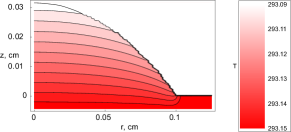
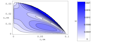
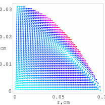
Figure 1: Temperature distribution, distribution of absolute value of velocity and vector field plot of velocity for a droplet of 1-hexanol in a single-vortex regime obtained for $\theta=35^{\circ}$, $k_{R}=1$, $h_{R}=h_{S}/R=0.05$.

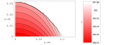
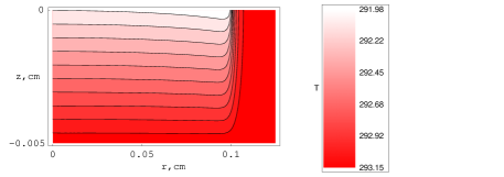
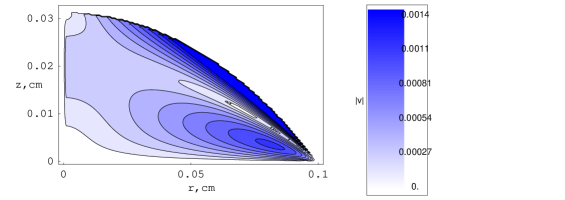
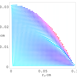
Figure 2: Temperature distribution inside the droplet and the substrate correspondingly, distribution of absolute value of velocity and vector field plot of velocity in a reversed single-vortex regime obtained for 1-hexanol, $\theta=35^{\circ}$, $k_{R}=0.01$, $h_{R}=h_{S}/R=0.05$.

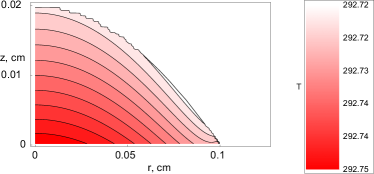
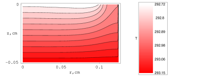
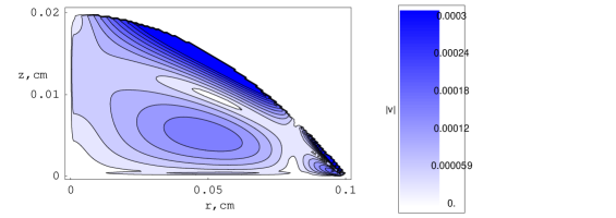
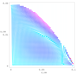
Figure 3: Temperature distribution inside the droplet and the substrate correspondingly, distribution of absolute value of velocity and vector field plot of velocity for a droplet of 1-hexanol in a two-vortex regime obtained for $\theta=22.44^{\circ}$, $k_{R}=0.2$, $h_{R}=h_{S}/R=0.5$.

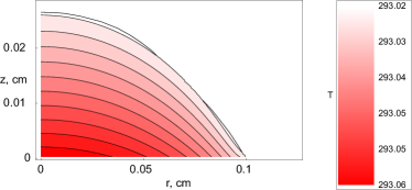
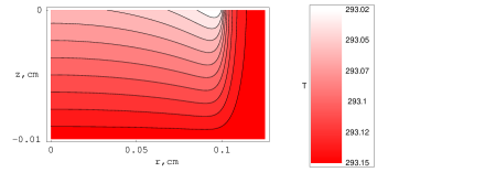
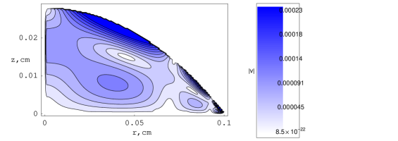
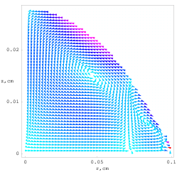
Figure 4: Temperature distribution inside the droplet and the substrate correspondingly, distribution of absolute value of velocity and vector field plot of velocity for a droplet of 1-hexanol in a three-vortex regime obtained for $\theta=31.22^{\circ}$, $k_{R}=0.2$, $h_{R}=h_{S}/R=0.1$.

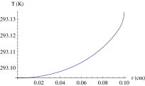
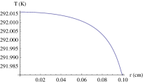
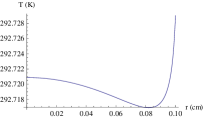
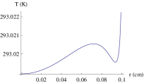
Figure 5: Surface temperature distribution for a single-vortex, reversed single-vortex, two-vortex and three-vortex regimes corresponding to the 1-hexanol droplets in Figs. 1-4.

In the second part of the method one takes $z$-derivative implicitly and represents Eqn. (3) as

$$\frac{T_{ij}^{n+1}-T_{ij}^{n+1/2}}{\kappa h_{t}/2}=\hat{\delta}_{r}^{2}T_{ij}^{n+1/2}+\hat{\delta}_{z}^{2}T_{ij}^{n+1}+\frac{1}{r}\frac{T_{i+1,j}^{n+1/2}-T_{i-1,j}^{n+1/2}}{a+b}.$$ (17)

For given temperature at time step $n+1/2$ this expression takes the form

$$c_{j}^{\prime\prime}T_{i,j-1}^{n+1}+(d_{j}^{\prime\prime}+2/(\kappa h_{t}))T_{ij}^{n+1}+e_{j}^{\prime\prime}T_{i,j+1}^{n+1}=c_{i}^{\prime}T_{i-1,j}^{n+1/2}+(d_{i}^{\prime}+2/(\kappa h_{t}))T_{ij}^{n+1/2}+e_{i}^{\prime}T_{i+1,j}^{n+1/2},$$ (18)

where the coefficients are given in (14)-(16). For each $i$ the tridiagonal matrix algorithm is used to solve the set of equations (18) for the temperature at time step $n+1$. The boundary condition $T^{n+1}_{S,i0}=T_{0}$, the boundary interpolation at the droplet surface (see below) and the matching condition $T_{i0}=c_{S}T_{i1}+c_{L}T_{S,i,n-1}$ are solved together with the set of equations (18) by the tridiagonal matrix algorithm, where $c_{S}=k_{L}h_{yS}/(k_{L}h_{yS}+k_{S}h_{yL})$, $c_{L}=1-c_{S}$. For $i>n$ the boundary condition at the substrate–gas interface is also used.

At the droplet surface we use the boundary interpolation. Consider a mesh point $D(i,j)$ close to the surface, where $j>1$. The point $D$ is inside the drop and at least one of its nearest neighbors is outside the drop. In linear approximation $T(r,z)=a+br+cz$ in a vicinity of the point $D(i,j)$. We denote the temperatures at points $D(i,j)$, $B(i-1,j)$ and $C(i,j-1)$ as $T_{D}$, $T_{B}$ and $T_{C}$ correspondingly; also let $G=\partial T/\partial n=-LJ(r)/k$ at a point $A$ of the drop surface near $D$. Then one has

$$b\sin\phi+c\cos\phi=G,\qquad a+b(i-1)h_{r}+cjh_{z}=T_{B},\qquad a+bih_{r}+c(j-1)h_{z}=T_{C}.$$ (19)

The solution of the set of equations is

$$a = \left(h_{r}\cos\phi(iT_{B}-(i-1)T_{C})+h_{z}\sin\phi(T_{B}+j(T_{C}-T_{B}))-h_{r}h_{z}G(j+i-1)\right)/R$$ (20)

$$b = (h_{z}G+(T_{C}-T_{B})\cos\phi)/R$$ (21)

$$c = (h_{r}G+(T_{B}-T_{C})\sin\phi)/R$$ (22)

$$R = h_{r}\cos\phi+h_{z}\sin\phi.$$ (23)

In the first part of the alternating direction method the calculations of rows proceed towards larger values of $j$. For this reason one should consider here $T_{C}$ and $G$ as given quantities, whereas $T_{B}$ and $T_{D}$ are unknown. It is convenient under these conditions to represent (20)-(23) as

$$a=a_{0}+a_{1}T_{B},\qquad b=b_{0}+b_{1}T_{B},\qquad c=c_{0}+c_{1}T_{B},$$ (24)

and obtain explicit expressions for $a_{0},a_{1},b_{0},b_{1},c_{0},c_{1}$. This results in linear relation between $T_{D}$ and $T_{B}$

$$T_{D}=a+br_{D}+cz_{D}=(a_{0}+b_{0}r_{D}+c_{0}z_{D})+(a_{1}+b_{1}r_{D}+c_{1}z_{D})T_{B},$$ (25)

which can be transformed to the form $d_{i-1}^{\prime}T_{i-1,j}^{n+1/2}+e_{i-1}^{\prime}T_{ij}^{n+1/2}=b_{i-1}^{\prime}$. This completes the set of equations (13) for the tridiagonal matrix algorithm. Here $d_{i-1}^{\prime}=-(a_{1}+b_{1}r_{D}+c_{1}z_{D})$, $e_{i-1}^{\prime}=1$, $b_{i-1}^{\prime}=a_{0}+b_{0}r_{D}+c_{0}z_{D}$.

To carry out the boundary interpolation in the second part of the alternating direction method, similar expressions can be derived to relate $T_{D}$ and $T_{C}$. A similar boundary interpolation method is also derived for $j\leq 1$.

III Results and discussions

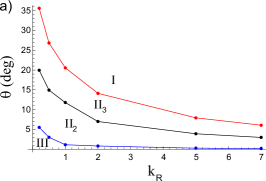
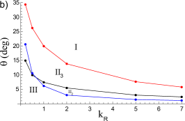
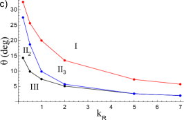
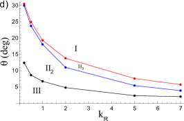
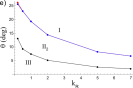
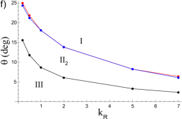
Figure 6: Results for $\theta$ vs $k_{R}=k_{S}/k_{L}$, where a) $h_{R}=0.01$, b) $h_{R}=0.05$, c) $h_{R}=0.1$, d) $h_{R}=0.2$, e) $h_{R}=0.5$, f) $h_{R}=1$.

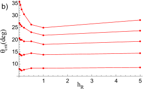
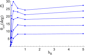
Figure 7: Dependence of $\theta_{crit}$ on $h_{R}=h_{S}/R$ for a) the transition corresponding to the change of sign of tangential component of the temperature gradient at the liquid–vapor interface near the contact line; b) the transition to a monotonically increasing surface temperature dependence on $r$; c) the transition corresponding to the change of sign of tangential component of the temperature gradient at the liquid–vapor interface near the droplet apex.

We have carried out the numerical simulation of the evaporation and fluid dynamics of droplets of capillary size and studied the dependence of the results on the characteristics of the substrate. The thermal conduction equation and the Navier–Stokes equations have been solved using the numerical method described in Section II, where the equations and the boundary conditions used are presented as well.

Figs. 1–5 show four different regimes of fluid flow structure in an evaporating sessile droplet. The parameter set used is taken for 1-hexanol and presented in Table 1, where the notations are also introduced. The single-vortex regime is shown in Fig. 1, the reversed single-vortex regime is shown in Fig. 2, the two-vortex regime is shown in Fig. 3, and the three-vortex regime is shown in Fig. 4. Figs. 1–4 demonstrate spatial temperature distributions both inside the droplet and the substrate, distributions of absolute value of the fluid velocity and vector field plots of the velocity. The temperature distributions inside the droplet and the substrate are shown separately in Figs. 2–4 because different temperature scales are used here for the fluid and for the substrate. Using both plot of the velocity absolute value and vector field plot of the velocity allow to give a thorough picture of the velocity distribution. The basic difference between the four regimes is summarized in Fig. 5, which shows the surface temperature distribution corresponding to the droplets in Figs. 1–4.

Since 1-hexanol is weakly volatile liquid, the evaporation process is comparatively slow, and the corresponding Péclet number $Pe=\overline{u}R/\kappa$ is much smaller than unity for the droplets of relatively small size considered (here $\overline{u}$ is a characteristic value of fluid velocity). The assumption $Pe\ll 1$ is justified by the numerical results for the velocity values shown in the absolute value plots in Figs. 1–4. Hence, the convective heat transfer is negligibly small. Also we consider the evaporation as a quasistationary process, which is realized when the transient time for heat transfer $t_{\text{heat}}=R(h_{0}+h_{S})/\kappa$, transient time for momentum transfer $t_{\text{mom}}=\rho Rh_{0}/\eta$ and transient time for vapor phase mass transfer $t_{\text{mass}}=\rho_{\text{vap}}/\rho\cdot t_{f}$ are much smaller than the total drying time $t_{\text{f}}\approx 0.2\rho Rh_{0}/(Du_{\text{s}})$. Here $h_{0}$ is the droplet height and $h_{S}$ is the substrate thickness. In addition, the droplet shape can be described with good accuracy within the spherical cap approximation when the capillary number $Ca=\eta\overline{u}/\sigma$ and the Bond number $Bo=\rho gh_{0}R/(2\sigma\sin\theta)$ are much smaller than unity Barash2009 .

Since driving forces for fluid convection are the Marangoni forces and $\partial\sigma/\partial T<0$, the fluid usually flows from a surface region with higher temperature to that with lower temperature. Therefore, the single-vortex flow corresponds to a surface temperature, which monotonically increases with increasing the axial coordinate $r$ (see Figs. 1,5). The reversed single-vortex flow (see Figs. 2,5) corresponds to a monotonically decreasing surface temperature dependence on $r$. The surface temperature, which induces a two-vortex or three-vortex flow, is found to be a nonmonotonic function of $r$ with a single extremum (in addition to extrema at the apex and at the contact line) in the two-vortex case and with both maximal and minimal values in the three-vortex case (see Figs. 3–5). Fig. 5 shows surface temperature distributions for the droplets in Figs. 1–4. We do not aim at listing all possible types of surface temperature distribution in Fig. 5. Also commonly observed is a two-vortex situation with a negative derivative at the edge, positive derivative at the apex, and a sign change in slope elsewhere, which is not shown in Fig. 5.

The parameter regions of different types of surface temperature distribution are shown in Fig. 6 in the form of the “phase diagram” in the $k_{R}$–$\theta$ plane, taken for various values of the substrate thickness. One can see that the region II of a nonmonotonic spatial dependence of the surface temperature consists of two regions. One of them, II₂, identifies surface temperature distributions with a single intermediate extremum, while another one, II₃, identifies surface temperature distributions with both maximal and minimal values. II₂ usually correspond to the two-vortex flows, while II₃ corresponds to the flows with three vortices. Black curve in Fig. 6 corresponds to the change of sign of the tangential component of temperature gradient at the liquid–vapor interface near the contact line. Blue curve in Fig. 6 corresponds to the change of sign of the tangential component of temperature gradient at the liquid–vapor interface at the droplet apex. Red curve in Fig. 6 corresponds to the transition between a nonmonotonic dependence of surface temperature on $r$ and a monotonically increasing surface temperature dependence on $r$.

The “phase diagram” shows that the regime of convection changes during the evaporation process when the contact angle diminishes. For example, when $k_{R}$ is large, three vortices can appear at relatively small contact angles (see also Barash2009 ).

The main features of a “phase diagram” can be qualitatively understood as a result of matching the heat transfer through the solid–liquid interface and the heat flowing through the liquid–vapor interface, which is associated with evaporative cooling. When $k_{R}$ is small, the evaporative cooling is much stronger than the heat flow from the substrate. Since an inhomogeneous evaporation rate $J_{s}(r)=J_{0}(\theta)(1-r^{2}/R^{2})^{-\lambda(\theta)}$ has its minimum at the apex, the surface region near the apex should be warmer than at the contact line. Thus, $k_{R}\ll 1$ results in a monotonic decrease of the surface temperature with $r$, which corresponds to the reversed single-vortex regime, i.e., to the region III of the “phase diagram”. If, on the contrary, $k_{R}\gg 1$, then the heat flowing through the solid–liquid interface is much stronger than the heat flow due to evaporative cooling. Therefore, the area of liquid–vapor interface close to the contact line is the warmest one due to adjacent highly conducting substrate. In this case the surface area close to the apex is colder as compared to other parts of the droplet. Thus, $k_{R}\gg 1$ results in a monotonic increase of the surface temperature with $r$, which corresponds to the single-vortex region I of the “phase diagram”. We also note that the increase of the nonuniform evaporation rate $J_{s}(r)=J_{0}(\theta)(1-r^{2}/R^{2})^{-\lambda(\theta)}$ near the contact line becomes more pronounced with decreasing the contact angle, since $\lambda(\theta)=1/2-\theta/\pi$. For this reason, at small contact angles the heat flow due to evaporative cooling usually dominates near the contact line and results in the reversed single-vortex region III of the “phase diagram”. At large contact angles, the heat flow from the substrate has much more chances to dominate, and this results in the region I of the “phase diagram”.

We also study the dependence of the fluid flows on the thickness of the substrate. Fig. 6 shows the “phase diagram” obtained for different values of $h_{R}=h_{S}/R$. As seen in Fig. 6, with an increase of the substrate thickness, the subregion II₂ becomes dominating in the region II. Further increase of the substrate thickness results in shifting the regions I and II to larger contact angles. The blue curve in Fig. 6 is situated below the black curve at small values of $h_{R}$, while at larger values of $h_{R}$ it is above the black curve. Therefore, the transition between the regions III and II₂ corresponds to the change of sign of the tangential component of the temperature gradient at the liquid–vapor interface either at the droplet apex (for small substrate thickness) or near the contact line (for larger substrate thickness). The transition between the regions II₂ and II₃ corresponds to the change of sign of the tangential component of the temperature gradient at the liquid–vapor interface either near the contact line (for small substrate thickness) or at the droplet apex (for larger substrate thickness). Fig. 7 shows the dependence of $\theta_{crit}$ on $h_{R}$ for the transitions between the regions I, II₂, II₃ and III. A behavior of critical angles as a function of $h_{R}$ shown in Fig. 7 is, naturally, different in the region $h_{R}\lesssim 0.1$, where the blue curve is below the black curve in Fig. 6, and in the region $h_{R}\gtrsim 0.1$, where it is above the black curve.

IV Conclusions

The fluid flow structure in an evaporating sessile droplet of capillary size has been considered in disregarding the convective heat transfer, i.e., for relatively small and slowly evaporating droplets (when $Pe=\overline{u}R/\kappa\ll 1$). It is shown that the region II of the “phase diagram” introduced in Zhang consists of the two subregions II₂ and II₃, where II₂ corresponds to the flows with two vortices and II₃ corresponds to the flows with three vortices. The transition between the regions III and II₂ corresponds to the change of sign of the tangential component of the temperature gradient at the liquid–vapor interface either at the droplet apex (for small substrate thickness) or near the contact line (for larger substrate thickness). The transition between the regions II₂ and II₃ corresponds to the change of sign of the tangential component of the temperature gradient at the liquid–vapor interface either near the contact line (for small substrate thickness) or at the droplet apex (for larger substrate thickness). Further increase of the substrate thickness makes subregion II₂ dominating in region II, and results in a shift of the regions I and II to larger contact angles.

Temperature distribution, fluid flow structure in the droplet and general form of a “phase diagram” can be qualitatively understood as a result of matching the heat transfer through the solid–liquid interface and the heat flow due to evaporative cooling.

The results may provide a better understanding of the Marangoni effect of drying droplets and allow one to influence the fluid flow structure in evaporating droplets. The results may potentially be useful to better understand numerous experimental results on evaporative deposition patterns and self-assembly of colloids and other materials.

References

- (1)
- (2) R. D. Deegan, O. Bakajin, T. F. Dupont, G. Huber, S. R. Nagel, T. A. Witten, Nature 389, 827 (1997).
- (3) R. D. Deegan, O. Bakajin, T. F. Dupont, G. Huber, S. R. Nagel, T. A. Witten, Contact line deposits in an evaporating drop, Phys. Rev. E 62, 756 (2000).
- (4) H.Y. Erbil, Evaporation of pure liquid sessile and spherical suspended drops: A review, Adv. Colloid Int. Sci. 170, 67 (2012).
- (5) R.G. Larson, Transport and deposition patterns in drying sessile droplets, AIChE Journal 60(5), 1538 (2014).
- (6) J. Park, J. Moon, Control of Colloidal Particle Deposit Patterns within Picoliter Droplets Ejected by Ink-Jet Printing Langmuir 22, 3506 (2006).
- (7) P. Calvert, Inkjet Printing for Materials and Devices, Chem. Mater. 13, 3299 (2001).
- (8) Y. Yu, H. Zhu, J.M. Frantz, M.E. Reding, K.C. Chan, H.E. Ozkan, Evaporation and coverage area of pesticide droplets on hairy and waxy leaves, Biosystems. Eng. 104, 324 (2009).
- (9) D. Xia, S.R.J. Brueck, Strongly Anisotropic Wetting on One-Dimensional Nanopatterned Surfaces, Nano Lett 8, 2819 (2008).
- (10) G.T. Carroll, D. Wang, N.J. Turro, J.T. Koberstein, Photochemical Micropatterning of Carbohydrates on a Surface, Langmuir 22, 2899 (2006).
- (11) M. Kimura, M.J. Misner, T. Xu, S.H. Kim, T.P. Russell, Long-Range Ordering of Diblock Copolymers Induced by Droplet Pinning, Langmuir 19, 9910 (2003).
- (12) V.X. Nguyen, K.J. Stebe, Patterning of Small Particles by a Surfactant-Enhanced Marangoni-Bénard Instability, Phys Rev Lett 88, 164501 (2002).
- (13) W. Jia, H.-H. Qiu, Experimental investigation of droplet dynamics and heat transfer in spray cooling, Exp. Therm. Fluid. Sci. 27, 829 (2003).
- (14) D. Brutin, B. Sobac, B. Loquet, J. Sampol, Pattern formation in drying drops of blood, J. Fluid Mech. 667 85 (2011).
- (15) Trantum JR, Wright DW, Haselton FR. Biomarker-mediated disruption of coffee-ring formation as a low resource diagnostic indicator, Langmuir 28, 2187 (2012).
- (16) M. Schena, D. Shalon, R.W. Davis, P.O. Brown, Quantitative Monitoring of Gene Expression Patterns with a Complementary DNA Microarray, Science 270, 467 (1995).
- (17) X. Fang, B. Li, E. Petersen, Y.S. Seo, V.A. Samuilov, Y. Chen et al., Drying of DNA Droplets, Langmuir 22, 6308 (2006).
- (18) G. McHale, Surface free energy and microarray deposition technology, Analyst 132, 192 (2007).
- (19) T. Kawase, H. Sirringhaus, R.H. Friend, T. Shimoda, Inkjet Printed Via-Hole Interconnections and Resistors for All-Polymer Transistor Circuits, Adv. Mater. 13, 1601 (2001).
- (20) C. Sodtke, V.S. Ajaev, P. Stephan, Evaporation of thin liquid droplets on heated surfaces, Heat and Mass Transfer 43, 649 (2007).
- (21) L. Tarozzi, A. Muscio, P. Tartarini, Experimental tests of dropwise cooling in infrared-transparent media, Exp. Therm. and Fluid Sci., 31, 857 (2007).
- (22) D. N. Voylov, L. M. Nikolenko, D. Yu. Nikolenko, N. A. Voylova, E. M. Olsen, V. F. Razumov, Self-Assembly of charged CdTe nanoparticles, JETP Letters 95(12), 656 (2012).
- (23) Z. L. Wang, Structural analysis of self-assembling nanocrystal superlattices, Adv. Mater. 10, 13 (1998).
- (24) G. Ge, L. Brus, Evidence for spinodal phase separation in two-dimensional nanocrystal self-assembly, J. Phys. Chem. B 104, 9573 (2000).
- (25) Y. Cai, B. Z. Newby, Marangoni flow-induced self-assembly of hexagonal and stripelike nanoparticle patterns, J. Am. Chem. Soc. 130, 6076 (2008).
- (26) S. Narayanan, J. Wang, X. M. Lin, Dynamical self-assembly of nanocrystal superlattices during colloidal droplet evaporation by in situ small angle x-ray scattering, Phys. Rev. Lett. 93, 135503 (2004).
- (27) T. P. Bigioni, X. M. Lin, T. T. Nguyen, E. I. Corwin, T. A. Witten, H. M. Jaeger, Kinetically driven self assembly of highly ordered nanoparticle monolayers, Nature Materials 5, 265 (2006).
- (28) H. Hu, R.G. Larson, Marangoni effect reverses coffee-ring depositions, J Phys Chem B. 110, 7090 (2006).
- (29) R. Savino, S. Fico, Transient Marangoni convection in hanging evaporating drops, Phys. Fluids 16, 3738 (2004).
- (30) H. Hu, R. G. Larson, Analysis of the Effects of Marangoni Stresses on the Microflow in an Evaporating Sessile Droplet, Langmuir 21, 3972 (2005).
- (31) W. D. Ristenpart, P. G. Kim, C. Domingues, J. Wan, H. A. Stone, Influence of substrate conductivity on circulation reversal in evaporating drops, Phys. Rev. Lett. 99, 234502 (2007).
- (32) X. Xu, J. Luo, D. Guo, Criterion for Reversal of Thermal Marangoni Flow in Drying Drops, Langmuir 26(3), 1918 (2010).
-
(33)
L.Yu. Barash,
Dependence of the fluid convection in an evaporating sessile droplet on the thermal
conductivity of the substrate,
XXIII IUPAP Conference on Computational Physics (2011),
http://ccp2011.ornl.gov/pdf/Abstracts/Barash_Lev_9.1b_8.pdf - (34) K. Zhang, L. Ma, X. Xu, J. Luo, D. Guo, Temperature distribution along the surface of evaporating droplets, Phys. Rev. E 89, 032404 (2014).
- (35) L.Yu. Barash, T.P. Bigioni, V.M. Vinokur, L.N. Shchur, Evaporation and fluid dynamics of a sessile drop of capillary size, Phys. Rev. E 79, 046301 (2009).
- (36) H. Hu, R. G. Larson, Evaporation of a Sessile Droplet on a Substrate, J. Phys. Chem. B 106, 1334 (2002).
- (37) N. N. Lebedev, Special Functions and Their Applications (Prentice-Hall, Englewood Cliffs, NJ, 1965).
- (38) D. R. Lide, CRC Handbook of Chemistry and Physics (CRC Press, 2004).
- (39) N. A. Fuchs, Evaporation and droplet growth in gaseous media (Pergamon Press, Oxford, 1959).
- (40) Voevodin Vl.V., Zhumatiy S.A., Sobolev S.I., Antonov A.S., Bryzgalov P.A., Nikitenko D.A., Stefanov K.S., Voevodin Vad.V., Practice of ”Lomonosov” Supercomputer, Open Systems J., Moscow: Open Systems Publ., 2012, no.7. (In Russian)