Abstract

The U-curve optimization problem is characterized by a decomposable in U-shaped curves cost function over the chains of a Boolean lattice. This problem can be applied to model the classical feature selection problem in Machine Learning. Recently, the U-Curve algorithm was proposed to give optimal solutions to the U-curve problem. In this article, we point out that the U-Curve algorithm is in fact suboptimal, and introduce the U-Curve-Search (UCS) algorithm, which is actually optimal. We also present the results of optimal and suboptimal experiments, in which UCS is compared with the UBB optimal branch-and-bound algorithm and the SFFS heuristic, respectively. We show that, in both experiments, UCS had a better performance than its competitor. Finally, we analyze the obtained results and point out improvements on UCS that might enhance the performance of this algorithm.

Keywords: combinatorial optimization, branch and bound, feature selection, U-curve problem, machine learning, Boolean lattice

1 Introduction

The feature selection problem is a problem in Machine Learning that has been studied for many years (Theodoridis & Koutroumbas, 2006). It is a combinatorial optimization problem that consists in finding a subset $X$ of a finite set of features $S$ that minimizes a cost function $c$, defined from $\mathcal{P}(S)$, the power set of $S$, to $\mathbb{R}+$. If $X$ is a subset of $S$ and $c(X)$ is a minimum (i.e., there does not exist another subset $Y$ of $S$ such that $c(Y)<c(X)$), then $X$ is an optimal set of features or a set of features of minimum cost. The model of the feature selection problem is defined by a cost function that has impact in the complexity of the corresponding search algorithms. In realistic models, the cost function depends on the estimation of the joint probability distribution. The feature selection problem is NP-hard (Meiri & Zahavi, 2006), which implies that the search for a subset $X$ of $S$ of minimum cost maybe unfeasible (i.e., it may require a computing time that is exponential in the cardinality of $S$). However, for some families of cost functions, there is a guarantee that the problem is not NP-hard and, consequently, the search problem is feasible; for instance, when the cost function is submodular (Schrijver, 2000). Moreover, depending on the definition of the cost function, different search algorithms may be employed to solve the problem. Therefore, a feature selection problem relies on two important steps:

• the choice of an appropriate cost function, also known as feature selection subset criterion, which may lead to either a feasible or an unfeasible search problem;

• the choice of an appropriate feature subset selection search algorithm for the defined search problem. The chosen search algorithm may be either optimal (i.e., it always finds a subset of minimum cost) or suboptimal (i.e., it may not find a subset of minimum cost).

The central problem in Machine Learning is the design of classifiers from a given joint distribution of a vector of features and the corresponding labels. Usually, such joint distribution is estimated from a limited number of samples and the estimation error depends on the choice of the feature selection vector. A feature subset selection criterion is a measure of the estimated joint distribution that intends to identify the availability of small error classifiers. Some noteworthy feature subset selection criteria are the Kullback-Leibler distance, the Chernoff bound (Narendra & Fukunaga, 1977), the divergence distance, the Bhattacharyya distance (Piramuthu, 2004), and the mean conditional entropy (Lin, 1991). All those criteria are measures of the estimation of joint distribution of a feature subset (Barrera et al., 2007; Ris et al., 2010), therefore they are susceptible to the U-curve phenomenon; that is, for a fixed number of samples, the increase in the number of considered features may have two consequences: if the available sample is enough to a good estimation, then it should occur a reduction of the estimation error, otherwise, the lack of data induces an increase of the estimation error. In practice, the available data are not enough for good estimations. A criterion that is susceptible to the U-curve phenomenon has U-shaped graphs when the function domain is restricted to a chain of the Boolean lattice $(\mathcal{P}(S),\subseteq)$. Such criterion may be used as the cost function of a U-curve problem, which models a feature selection problem.

A feature subset selection algorithm is a search algorithm on the space $\mathcal{P}(S)$ under the cost function $c$. Some mechanisms of a general search algorithm are: an order to visit the elements of $\mathcal{P}(S)$; visit and measure an element $X$ of $\mathcal{P}(S)$; compare $c(X)$ with the current minimum and update the minimum if necessary; prune every known element $Y$ of $\mathcal{P}(S)$ such that $c(Y)>c(X)$; stop when the current minimum satisfies a given condition. Once it is unknown a polynomial-time optimal algorithm for the feature subset selection problem, some heuristics that produce suboptimal solutions are applied (Pudil et al., 1994; Meiri & Zahavi, 2006; Unler & Murat, 2010). One of the first introduced heuristics was the sequential selection: Marill & Green (1963) presented a feature selection algorithm for instances whose cost functions were determined by a divergence distance. This greedy algorithm, named Sequential Backward Selection (SBS), is feasible, though it has the so called “nesting effect” (Pudil et al., 1994). Whitney (1971) introduced the dual of the SBS, the Sequential Forward Selection (SFS) algorithm, which also has the nesting effect. Some heuristics were proposed in order to deal with the nesting effect (Kittler, 1978), among them the Sequential Forward Floating Selection (SFFS) introduced by Pudil et al. (1994). In the following years, several works were published suggesting improvements on the SFFS algorithm (Somol et al., 1999; Nakariyakul & Casasent, 2009). Nevertheless, the probability that a sequential selection based algorithm gives an optimal solution decreases with the increase of the number of features of the problem (Kudo & Sklansky, 2000), which encourages the investigation of algorithms that give an optimal solution, a much less explored family of feature selection algorithms  (Jain & Mao, 2000). Narendra & Fukunaga (1977) presented a branch-and-bound algorithm for the feature selection problem with cost functions that are increasing. As in the exhaustive search, the algorithm always gives an optimal solution, although it may be unfeasible for a big number of features (Pudil et al., 1994; Ris et al., 2010). Ris et al. (2010) proposed a search algorithm to solve the U-curve problem, the U-Curve algorithm.

The remainder of this article is organized as follows: in Section 2, we formalize the U-curve problem, point out an error in the U-Curve algorithm introduced by Ris et al, and present a modification to fix it. This correction implies in the creation of a new optimal-search algorithm for the U-curve problem, the U-Curve-Search (UCS) algorithm. In Section 3, we show some experimental results with UCS, the UBB optimal branch-and-bound algorithm, and the SFFS heuristic, and make a comparative analysis under optimal and suboptimal conditions. In Section 4, we present some analyses on the theoretical and experimental results. Finally, in Section 5, we point out the contributions of this paper and suggest some future works for this research.

2 The U-Curve and the U-Curve-Search algorithms

Let $S$ be a finite non-empty set. The power set $\mathcal{P}(S)$ is the collection of all subsets of $S$, including the empty set and $S$ itself. A chain is a collection $\{X_{1},X_{2},\ldots,X_{k}\}\subseteq\mathcal{P}(S)$, such that $X_{1}\subseteq X_{2}\subseteq\ldots\subseteq X_{k}$. A chain of $\mathcal{P}(S)$ is maximal if it is not properly included by any other chain of $\mathcal{P}(S)$. Let $\mathcal{X}\subseteq\mathcal{P}(S)$ be a chain and $f$ be a function that takes values from $\mathcal{X}$ to $\mathbb{R}+$. $f$ describes a U-shaped curve if, for any $X_{1},X_{2},X_{3}\in\mathcal{X}$, then $X_{1}\subseteq X_{2}\subseteq X_{3}$ implies that $f(X_{2})\leq max\{f(X_{1}),f(X_{3})\}$. A cost function $c$ is a function defined from $\mathcal{P}(S)$ to $\mathbb{R}+$. $c$ is decomposable in U-shaped curves if, for each chain $\mathcal{X}\subseteq\mathcal{P}(S)$, the restriction of $c$ to $\mathcal{X}$ describes a U-shaped curve. Let $X$ be an element of $\mathcal{X}\subseteq\mathcal{P}(S)$. If there does not exist another element $Y$ of $\mathcal{X}$ such that $c(Y)<c(X)$, then $X$ is of minimum cost in $\mathcal{X}$. If $\mathcal{X}=\mathcal{P}(S)$, then we just say that $X$ is of minimum cost.

Now let us define the central problem that is studied in this article.

Problem 2.1.

(U-curve problem) Given a non-empty set $S$ and a decomposable in U-shaped curves cost function $c$, find an element of $\mathcal{P}(S)$ of minimum cost.

2.1 The U-Curve algorithm

Let $S$ be a finite non-empty set. An interval $[A,B]$ of $\mathcal{P}(S)$ is defined as $[A,B]:=\{X\in\mathcal{P}(S):A\subseteq X\subseteq B\}$. Let $[\emptyset,L]$ be an interval with the leftmost term being the empty set. $L$ is a lower restriction. In the same way, let $[U,S]$ be an interval with the rightmost term being the complete set. $U$ is an upper restriction. An element of $\mathcal{P}(S)$ may be represented by the characteristic vector in $\{0,1\}^{|S|}$. In the figures of this article, every Boolean lattice has its elements described through their characteristic vectors.

Aiming to solve the U-curve optimization problem (problem 2.1), Ris et al. (2010) presented the U-Curve algorithm. The U-Curve is an optimal algorithm that has the following properties:

1. it works on a search space (the collection of subsets of a finite, non-empty set) that is a Boolean lattice;

2. and optimizes cost functions that are decomposable in U-shaped curves.

The way the U-Curve algorithm visits the search space takes into account the properties (i) and (ii): at each iteration, the algorithm explores a maximal chain, either in bottom-up or top-down way, until it reaches an element $M$ of minimum cost. Then, it executes a procedure, called “minimum exhausting”, that performs a depth-first search for elements of cost less or equal to $c(M)$. At the end of the iteration, a list of elements of minimum cost visited so far is updated and the search space is reduced through the update of two collections of elements, called “upper restrictions” and “lower restrictions”. Each element $U$ of the “upper restrictions” removes from the search space the elements in the interval $[U,S]$, while each element $L$ of the “lower restrictions” removes from the search space the elements in the interval $[\emptyset,L]$. The algorithm performs a succession of iterations until the search space is empty. For a detailed explanation of the algorithm dynamics, refer to Ris et al. (2010), particularly to Figure 4.

The U-Curve algorithm showed a better performance than the SFFS heuristic, that is, for a given instance of the U-curve problem, U-Curve finds subsets of cost less or equal to the best subset found by SFFS, generally with fewer access to the cost function  (Ris et al., 2010). To avoid unnecessary access to cost function usually is important in feature selection problems, since often one access is expensive and the search space is very large.

2.2 Problem with the U-Curve algorithm

Although the U-Curve algorithm was designed to be optimal, an analysis of its correctness resulted in the discovery of a problem that leads to suboptimal results in some kinds of instances. This problem is located in the Minimum-Exhausting subroutine, which is described in Ris et al. (2010), Algorithm 3. Minimum-Exhausting performs a depth-first search (DFS) on the Boolean lattice. The subroutine begins by adding into a stack an element that has minimum cost in a given chain of $\mathcal{P}(S)$. Let us call $T$ the top of this stack. At the beginning of each iteration, all elements adjacent to $T$ in the graph defined by the Hasse diagram of the lattice are evaluated, that is, all elements that have Hamming distance one to $T$. Then, from those elements adjacent to $T$, we push into the stack every element $Y$ that satisfies the conditions: (i) $Y$ was not removed from the search space by the collections of restrictions; (ii) $Y$ has a cost less or equal than $T$; (iii) $Y$ is not in the stack. If no adjacent element of $T$ was added into the stack, then $T$ is considered a “minimum exhausted”, which implies that it is popped from the stack and added to the collections of lower and upper restrictions, ending this iteration. The subroutine iterates until the stack is empty.

We will show now that Minimum-Exhausting has an error that may lead to suboptimal results. In Figure 1, we show an example of an instance $\langle S,c\rangle$ of the U-curve problem, in which the element of the Boolean lattice with minimum cost may be lost during the execution of the Minimum-Exhausting subroutine. This subroutine is called in Figure 1, in which the DFS procedure starts pushing $11100$ into the stack. The search branches until the element $01110$ is pushed into the stack; once $01110$ has no adjacent element out of the stack, the subroutine backtracks to the element $01111$ (Figure 1). The element $01111$ also has no element out of the stack, therefore it is popped from the stack and included in the collections of restrictions – this operation removes from the search space the unique global minimum, $00001$, which was not visited yet, thus losing it (Figure 1).

2.3 The principles of the proposed correction

We will now present the principles of the proposed correction by providing sufficient conditions to remove unvisited elements from the search space without losing global minima. In the following, we show four sufficient conditions for removing elements from the search space.

Proposition 2.2.

Let $\langle S,c\rangle$ be an instance of the U-curve problem, $\mathcal{X}\subseteq\mathcal{P}(S)$ be a current search space, and $X$ be an element of $\mathcal{X}$. If there exists an element $Y\in\mathcal{X}$ such that $Y\subseteq X$ and $c(Y)>c(X)$, then all elements in $[\emptyset,Y]$ have cost greater than $c(X)$.

Proof.

Let us consider $X,Y\in\mathcal{P}(S)$ and $Z\in[\emptyset,Y]$ such that $Y\subseteq X$ and $c(Y)>c(X)$. By the definition of a decomposable in U-shaped curves cost function, it holds that $c(Y)\leq max\{c(Z),c(X)\}$. Thus, $c(Y)\leq c(Z)$ or $c(Y)\leq c(X)$, and $c(Y)>c(X)$. Therefore, we have $c(Z)\geq c(Y)>c(X)$, then that all elements in $[\emptyset,Y]$ have cost greater than $c(X)$. ∎

The result of Proposition 2.2 also holds for the Boolean lattice $(\mathcal{P}(S),\supseteq)$.

Proposition 2.3.

Let $\langle S,c\rangle$ be an instance of the U-curve problem, $\mathcal{X}\subseteq\mathcal{P}(S)$ be a current search space, and $X$ be an element of $\mathcal{X}$. If there exists an element $Y\in\mathcal{X}$ such that $X\supseteq Y$ and $c(X)>c(Y)$, then all elements in $[Y,S]$ have cost greater than $c(X)$.

Proof.

Applying the principle of duality, the result of Proposition 2.2 also holds for the Boolean lattice $(\mathcal{P}(S),\supseteq)$. ∎

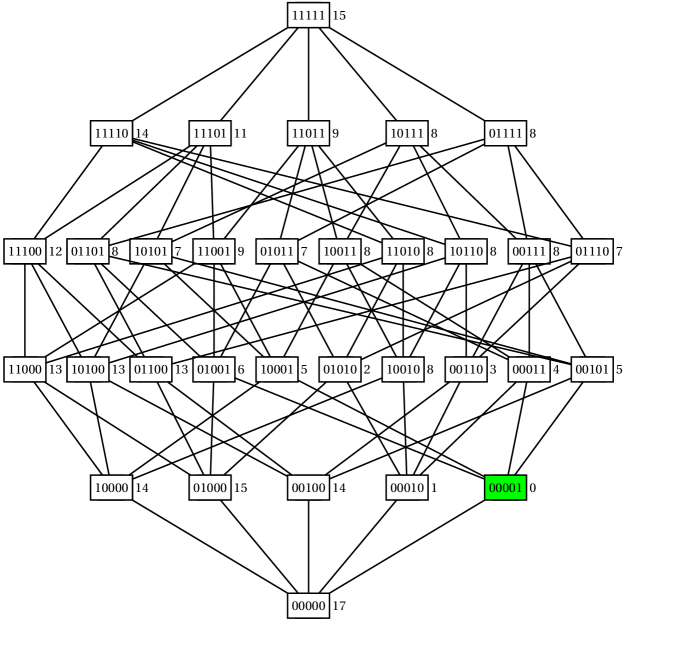
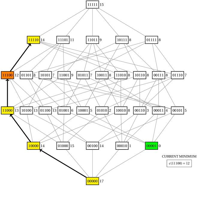
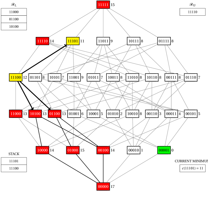
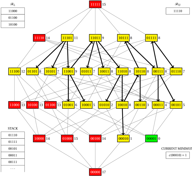
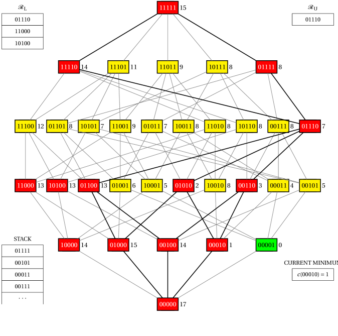
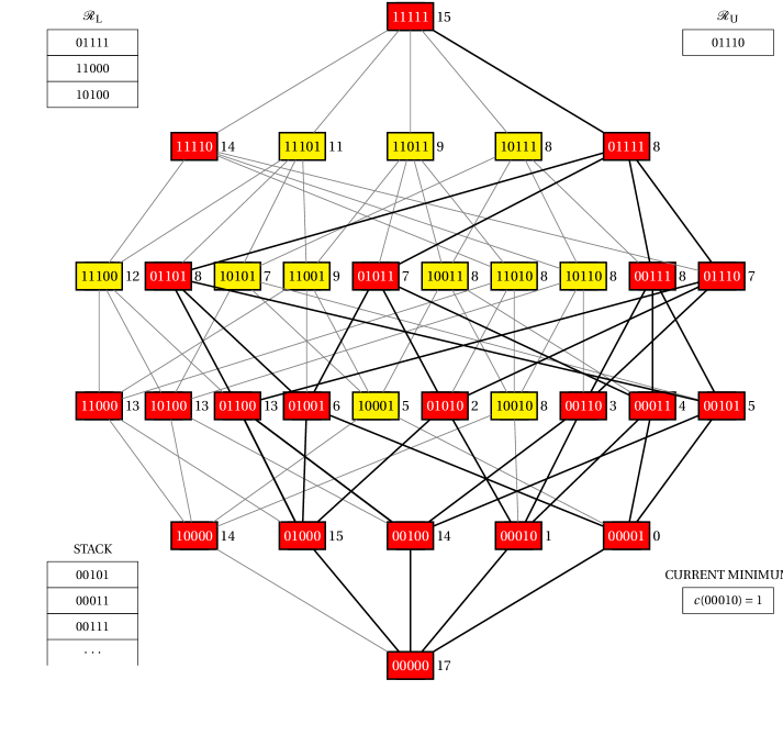
Figure 1: a counter-example of the correctness of Minimum-Exhausted subroutine. In this simulation of the subroutine, visited elements are in yellow, while elements that were removed from the search space are in red. In Fig. 1, a pruning removes from the search space the global minimum, thus losing it.

Let $A$ and $B$ be elements of $\mathcal{P}(S)$. $A$ is lower adjacent to $B$ (and $B$ is upper adjacent to $A$) if $A\subseteq B$ and there is no element $X\in\mathcal{P}(S)$ such that $A\subset X\subset B$. There is a basic result in Boolean algebra that also guarantees the removal of one element from the search space without the risk of losing global minima.

Proposition 2.4.

Let $S$ be a non-empty set, $\mathcal{X}\subseteq\mathcal{P}(S)$ be a current search space, and $X$ be an element of $\mathcal{X}$. If for each element $Y\in\mathcal{P}(S)$ such that $Y$ is lower adjacent to $X$, $[\emptyset,Y]\cap\mathcal{X}=\emptyset$, then $[\emptyset,X]-\{X\}$ does not contain an element of $\mathcal{X}$.

Proof.

Let us consider an element $X\in\mathcal{X}$ and that, for each element $Y\in\mathcal{P}(S)$ such that $Y$ is lower adjacent to $X$, $[\emptyset,Y]\cap\mathcal{X}=\emptyset$. Due to the fact that $X$ is the least upper bound of its lower adjacent elements, $\cup\{[\emptyset,Y]:Y\mbox{ is lower adjacent to }X\}=[\emptyset,X]-X$. Therefore, $[\emptyset,X]-\{X\}$ does not contain an element of $\mathcal{X}$. ∎

The result of Proposition 2.4 also holds for the Boolean lattice $(\mathcal{P}(S),\supseteq)$.

Proposition 2.5.

Let $S$ be a non-empty set, $\mathcal{X}\subseteq\mathcal{P}(S)$ be a current search space, and $X$ be an element of $\mathcal{X}$. If for each element $Y\in\mathcal{P}(S)$ such that $Y$ is upper adjacent to $X$, $[Y,S]\cap\mathcal{X}=\emptyset$, then $[X,S]-\{X\}$ does not contain an element of $\mathcal{X}$.

Proof.

Applying the principle of duality, the result of Proposition 2.4 also holds for the Boolean lattice $(\mathcal{P}(S),\supseteq)$. ∎

To fix the error in the Minimum-Exhausting subroutine, we developed a new optimal search algorithm for the U-curve problem. This new algorithm stores an element that is visited during a search in a structure called node. A node contains an element of $\mathcal{P}(S)$ and two Boolean flags: “lower restriction flag” and “upper restriction flag”, which assign whether the element of the node was removed from the search space, respectively, by the collection of lower restrictions or by the collection of upper restrictions. The algorithm also takes into account Propositions 2.2, 2.3, 2.4 and 2.5 to remove elements from the search space. There are two types of removal of elements from the search space:

• let $X$ and $Y$ be elements in $\mathcal{X}\subseteq\mathcal{P}(S)$, such that $Y$ is lower (in the dual case, upper) adjacent to $X$. If $c(Y)>c(X)$, then by Proposition 2.2 (2.3) the interval $[\emptyset,Y]$ ($[Y,S]$) should be removed from the search space. Therefore, $Y$ is included in the collection of lower (upper) restrictions and its node is marked with the lower (upper) restriction flag.

• let $X$ be an element in $\mathcal{X}\subseteq\mathcal{P}(S)$. If there is no element lower (in the dual case, upper) adjacent to $X$ in $\mathcal{X}$, then by Proposition 2.4 (2.5) the interval $[\emptyset,X]$ ($[X,S]$) should be removed from the search space. Therefore, $X$ is handled as the element $Y$ of the previous item.

In Figure 2, we show the first steps of a simulation of this new algorithm; the complete simulation is provided in the Supplementary Material.

2.4 The U-Curve-Search algorithm

In this section, we will present the U-Curve-Search (UCS) algorithm, which implements the proposed correction presented in the previous section. We will also give the time complexity of the main algorithm. The description of this algorithm will be done following a logical decomposition of the algorithm in a bottom-up way, that is, the subroutines will be presented and studied in the inverse order of the subroutine order call tree. The presentation of each subroutine will be given through its description and pseudo-code; the descriptions of dual subroutines will be omitted, as well as the pseudo-codes of very simple subroutines.

From now on, the cardinality of a non-empty set $S$ will be denoted as $n:=|S|$. It is assumed that any element $X\in\mathcal{P}(S)$ demands $n$ bits to represent it, and that any collection $\mathcal{R}\subseteq\mathcal{P}(S)$ is implemented using a doubly linked list. Therefore, the time complexity of a search is $O(n|\mathcal{R}|)$, of an insertion is $O(1)$, and of a deletion is $O(1)$. Finally, we assume that any call of the cost function $c$ demands $O(f(n))$, in which $f(n)$ depends on the chosen cost function.

2.4.1 Update of upper and lower restrictions

Let $X$ be an element in $\mathcal{P}(S)$. $X$ is covered by a collection of lower (in the dual form, upper) restrictions $\mathcal{R}_{L}$ ($\mathcal{R}_{U}$) if there exists an element $R\in\mathcal{R}_{L}$ ($R\in\mathcal{R}_{U}$) such that $X\subseteq R$ ($R\subseteq X$).

Subroutine description

Update-Lower-Restriction receives an element $X\in\mathcal{P}(S)$ and a collection of lower restrictions $\mathcal{R}_{L}$. If $X$ is not covered by $\mathcal{R}_{L}$, then the algorithm adds $X$ into $\mathcal{R}_{L}$ and removes all the elements of $\mathcal{R}_{L}$ that are properly contained in $X$. Finally, the subroutine returns the updated collection $\mathcal{R}_{L}$.

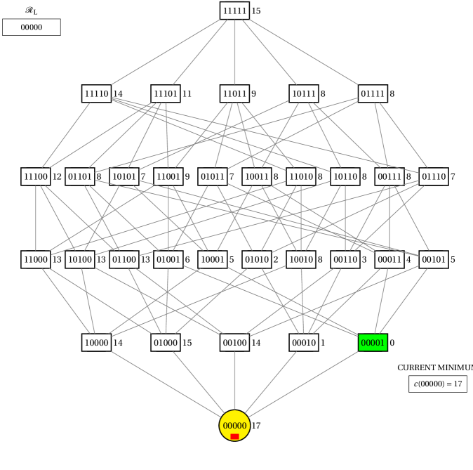
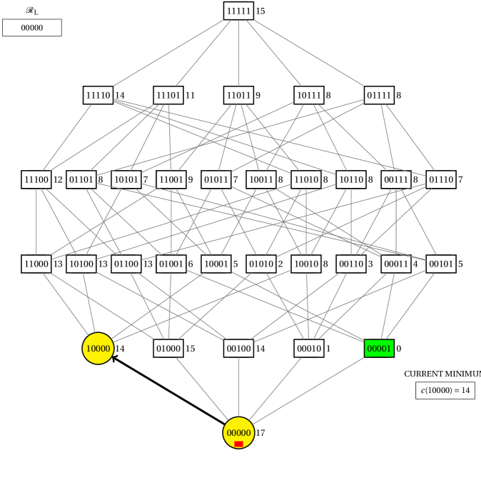
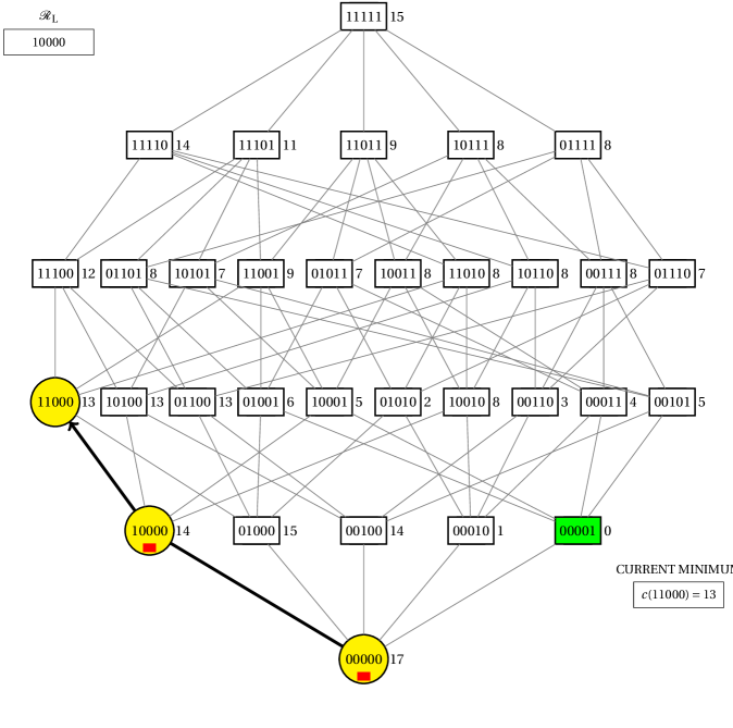
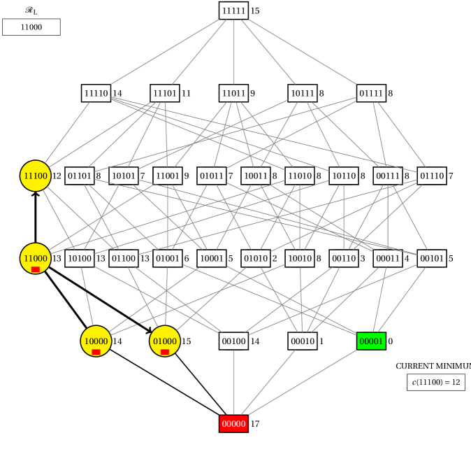
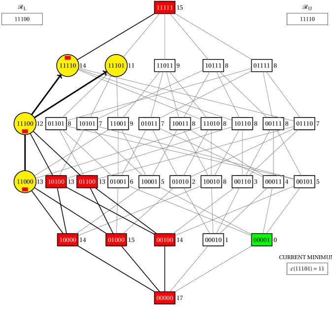
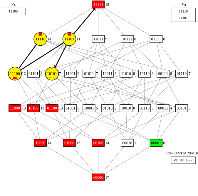
Figure 2: a simulation of the UCS algorithm. 2: the selection of a minimal element in the search space; 2– 2: first five iterations of the DFS subroutine; at each iteration, a visited element is either included in the collection of nodes (yellow circles) or is used for pruning. A lower (upper) red bar inside a yellow circle assigns that the node’s element is in the collection of lower (upper) restrictions $\mathcal{R}_{L}$ ($\mathcal{R}_{U}$).

2.4.2 Minimal and maximal elements

Let $X$ be an element of $\mathcal{A}\subseteq\mathcal{P}(S)$. $X$ is minimal (in the dual form, maximal) in $\mathcal{A}$ if for any $Y\in\mathcal{A}$, $Y\subseteq X$ ($X\subseteq Y$) implies that $X=Y$.

Now let $\mathcal{X}$ be a function that takes values from $\mathcal{P}(S)\times\mathcal{P}(S)$ to $\mathcal{P}(S)$, defined as

$\mathcal{X}(\mathcal{R}_{L},\mathcal{R}_{U})=\mathcal{P}(S)-\bigcup\{[\emptyset,R]:R\in\mathcal{R}_{L}\}-\bigcup\{[R,S]:R\in\mathcal{R}_{U}\}$.

We say that $\mathcal{X}(\mathcal{R}_{L},\mathcal{R}_{U})$ is a current search space of the search space $\mathcal{P}(S)$.

Subroutine description

Minimal-Element receives a set $S$ and a collection of lower restrictions $\mathcal{R}_{L}$. If the current search space $\mathcal{X}(\mathcal{R}_{L},\emptyset)$ is not empty, then the subroutine returns an element $X$ that is minimal in $\mathcal{X}(\mathcal{R}_{L},\emptyset)$; otherwise, it returns $NIL$.

Ris et al. (2010) provided an implementation of this subroutine (Algorithm $4$).

2.4.3 Depth-first search

Now, we will describe the depth-first search procedure that is called at each iteration of the UCS algorithm. We will start describing a data structure to store elements of $\mathcal{P}(S)$ and the flags described in Section 2.3. A node is a structure with four variables, of which all of them map to an element of $\mathcal{P}(S)$:

• “element” represents an element of $\mathcal{P}(S)$;

• “unverified” is used by the search algorithm to keep track of which element adjacent to “element” in the Boolean lattice was verified or not;

• “lower_adjacent” and “upper_adjacent” represent the topology of the current search space. If they are empty, then they are equivalent to, respectively, the “lower restriction flag” and “upper restriction flag” presented in Section 2.3;

Let $\mathcal{G}$ be a collection of nodes, $\mathbf{Y}$ be a node in $\mathcal{G}$, and $\mathcal{X}(\mathcal{R}_{L},\mathcal{R}_{U})$ be a current search space. Now, we will define three rules of the kernel of this subroutine dynamics:

1. Criterion to stop a search. If there is an element $X\in\mathcal{X}(\mathcal{R}_{L},\mathcal{R}_{U})$ adjacent to $\mathbf{Y}[element]$ such that $\mathbf{X}[element]\neq X$ for all node $\mathbf{X}$ in $\mathcal{G}$, then $X$ is an unvisited adjacent element to $\mathbf{Y}[element]$;

2. Management of the restriction flags. Given a $X$ in $\mathcal{P}(S)$ such that $X$ is lower (upper) adjacent to $\mathbf{Y}[element]$, if the unique element in $\mathbf{Y}[element]-X$ ($X-\mathbf{Y}[element]$) is not in $\mathbf{Y}[lower\_adjacent]$ ($\mathbf{Y}[upper\_adjacent]$), then $\mathcal{R}_{L}$ ($\mathcal{R}_{U}$) covers $X$.

   This rule describes an implementation of the “upper restriction flag” and “lower restriction flag” presented in Section 2.3, in a way that they also store information for the verification of the conditions of Propositions 2.4 and 2.5;

3. Management of visited adjacent elements. If $X$ is an unvisited adjacent element to $\mathbf{Y}$, then $\mathbf{Y}[unverified]$ has an element $y$ such that either $X=\mathbf{Y}[element]\cup\{y\}$ or $X=\mathbf{Y}[element]-\{y\}$ holds.

   This rule defines a way to avoid that, for each time it is verified if $\mathbf{Y}$ has an unvisited adjacent element, one must inspect all adjacent elements to $\mathbf{Y}[element]$ in $\mathcal{P}(S)$;

We will present now three subroutines that are used by the main DFS algorithm: the first one provides selection of an unvisited adjacent element; the second one provides lower pruning; the third one provides a pruning that takes into account the conditions of Propositions 2.2 and 2.3.

Subroutine description

Select-Unvisited-Adjacent receives a node $\mathbf{Y}$, a collection of nodes $\mathcal{G}$, a set $S$, a collection of lower restrictions $\mathcal{R}_{L}$, and a collection of upper restrictions $\mathcal{R}_{U}$. This subroutine searches for an unvisited adjacent element to $\mathbf{Y}[element]$. It verifies the condition of rule (i): if an unvisited adjacent $X$ is found, then this subroutine returns a node containing it; otherwise, it returns $NIL$. During the search procedure, the flags of $\mathbf{Y}$ are updated following the rules (ii) and (iii); hence, this subroutine also returns $\mathbf{Y}$.

• $\textnormal{Select-Unvisited-Adjacent}(\mathbf{Y},\mathcal{G},S,\mathcal{R}_{L},\mathcal{R}_{U})$
      1while $\mathbf{Y}[unverified]\neq\emptyset$ 2 doremove an element $y$ from $\mathbf{Y}[unverified]$ 3 if $y$ is in $\mathbf{Y}[element]$ 4 then $X\leftarrow\mathbf{Y}[element]-\{y\}$ 5 else $X\leftarrow\mathbf{Y}[element]\cup\{y\}$ 6 if $X$ is an unvisited adjacent to $\mathbf{Y}[element]$           $\rhd$ $\mathcal{G}$ is used in this test 7 then $\mathbf{X}[element]\leftarrow\mathbf{X}[lower\_adjacent]\leftarrow X$ 8 $\mathbf{X}[upper\_adjacent]\leftarrow S-X$ 9 $\mathbf{X}[unverified]\leftarrow S$ 10 return $\langle\mathbf{X},\mathbf{Y}\rangle$ 11 else if $X$ is lower adjacent to $\mathbf{Y}[element]$ and $X$ is covered by $\mathcal{R}_{L}$ 12 then $\mathbf{Y}[lower\_adjacent]\leftarrow\mathbf{Y}[lower\_adjacent]-(\mathbf{Y}[element]-X)$ 13 if $X$ is upper adjacent to $\mathbf{Y}[element]$ and $X$ is covered by $\mathcal{R}_{U}$ 14 then $\mathbf{Y}[upper\_adjacent]\leftarrow\mathbf{Y}[upper\_adjacent]-(X-\mathbf{Y}[element])$ 15return $\langle NIL,\mathbf{Y}\rangle$

Subroutine description

Lower-Pruning receives a node $\mathbf{Y}$, a collection of nodes $\mathcal{G}$, and a collection of lower restrictions $\mathcal{R}_{L}$. This subroutine includes $\mathbf{Y}[element]$ in $\mathcal{R}_{L}$ using the Update-Lower-Restriction subroutine. It also removes from $\mathcal{G}$ every node $\mathbf{X}$ such that $\mathbf{X}[element]$ is properly contained in $\mathbf{Y}[element]$. Finally, this subroutine returns the updated collections $\mathcal{G}$ and $\mathcal{R}_{L}$.

Subroutine description

Node-Pruning receives a pair of nodes $\mathbf{X}$ and $\mathbf{Y}$, a collection of nodes $\mathcal{G}$, a collection of lower restriction $\mathcal{R}_{L}$, a collection of upper restrictions $\mathcal{R}_{U}$, and a decomposable in U-shaped curves cost function $c$. It verifies the conditions of Propositions 2.2 and 2.3, pruning the collection of nodes and updating the collections of restrictions accordingly. Finally, it returns the updated collections $\mathcal{G}$, $\mathcal{R}_{L}$, and $\mathcal{R}_{U}$.

• $\textnormal{Node-Pruning}(\mathbf{X},\mathbf{Y},\mathcal{G},\mathcal{R}_{L},\mathcal{R}_{U},c)$
      1$X\leftarrow\mathbf{X}[element]\phantom{abcde}Y\leftarrow\mathbf{Y}[element]$ 2if $X$ is upper adjacent to $Y$ and $c(X)<c(Y)$ 3 then $\langle\mathcal{G},\mathcal{R}_{L}\rangle\leftarrow\textnormal{Lower-Pruning}(\mathbf{Y},\mathcal{G},\mathcal{R}_{L})$ 4 $\mathbf{X}[lower\_adjacent]\leftarrow\mathbf{X}[lower\_adjacent]-(X-Y)$ 5 $\mathbf{Y}[lower\_adjacent]\leftarrow\emptyset$ 6elseif $X$ is lower adjacent to $Y$ and $c(X)<c(Y)$ 7 then $\langle\mathcal{G},\mathcal{R}_{U}\rangle\leftarrow\textnormal{Upper-Pruning}(\mathbf{Y},\mathcal{G},\mathcal{R}_{U})$ 8 $\mathbf{X}[upper\_adjacent]\leftarrow\mathbf{X}[upper\_adjacent]-(Y-X)$ 9 $\mathbf{Y}[upper\_adjacent]\leftarrow\emptyset$ 10elseif $Y$ is upper adjacent to $X$ and $c(X)>c(Y)$ 11 then $\langle\mathcal{G},\mathcal{R}_{L}\rangle\leftarrow\textnormal{Lower-Pruning}(\mathbf{X},\mathcal{G},\mathcal{R}_{L})$ 12 $\mathbf{Y}[lower\_adjacent]\leftarrow\mathbf{Y}[lower\_adjacent]-(Y-X)$ 13 $\mathbf{X}[lower\_adjacent]\leftarrow\emptyset$ 14elseif $Y$ is lower adjacent to $X$ and $c(X)>c(Y)$ 15 then $\langle\mathcal{G},\mathcal{R}_{U}\rangle\leftarrow\textnormal{Upper-Pruning}(\mathbf{X},\mathcal{G},\mathcal{R}_{U})$ 16 $\mathbf{Y}[upper\_adjacent]\leftarrow\mathbf{Y}[upper\_adjacent]-(X-Y)$ 17 $\mathbf{X}[upper\_adjacent]\leftarrow\emptyset$ 18return $\langle\mathcal{G},\mathcal{R}_{L},\mathcal{R}_{U}\rangle$

The DFS main subroutine

Let $X$ be an element of $\mathcal{P}(S)$ and $c$ be a cost function decomposable in U-shaped curves. We want to perform a depth-first search in $\mathcal{X}(\mathcal{R}_{L},\mathcal{R}_{U})$ that starts with an element $Y$ and has as the depth-first criterion to expand the first element $X$ adjacent to $Y$ such that $X\in\mathcal{X}(\mathcal{R}_{L},\mathcal{R}_{U})$ and $c(X)\leq c(Y)$.

Subroutine description

DFS receives a non-empty set $S$, a node $\mathbf{M}$, a collection of lower restrictions $\mathcal{R}_{L}$, a collection of upper restrictions $\mathcal{R}_{U}$, and a decomposable in U-shaped curves cost function $c$. This subroutine performs a depth-first search using the criteria described above. The algorithm inspects a subset of the current search space $\mathcal{X}(\mathcal{R}_{L},\mathcal{R}_{U})$, update the current minima, and update the current search space to $\mathcal{X}(\mathcal{R^{\prime}}_{L},\mathcal{R^{\prime}}_{U})\subseteq\mathcal{X}(\mathcal{R}_{L},\mathcal{R}_{U})$. Therefore, the algorithm returns $\mathcal{R^{\prime}}_{L}$, $\mathcal{R^{\prime}}_{U}$, and a collection $\mathcal{M}$ containing every element $X$ in $\mathcal{X}(\mathcal{R}_{L},\mathcal{R}_{U})-\mathcal{X}(\mathcal{R^{\prime}}_{L},\mathcal{R^{\prime}}_{U})$ such that $X$ is a minimum in $\mathcal{X}(\mathcal{R}_{L},\mathcal{R}_{U})-\mathcal{X}(\mathcal{R^{\prime}}_{L},\mathcal{R^{\prime}}_{U})$.

• $\textnormal{DFS}(\mathbf{M},S,\mathcal{R}_{L},\mathcal{R}_{U},c)$
      1$\mathcal{M}\leftarrow\emptyset\phantom{abcde}\mathcal{G}\leftarrow\mathcal{S}\leftarrow\{\mathbf{M}\}$                 $\rhd$ $\mathcal{S}$ is a linked list 2while $\mathcal{S}\neq\emptyset$ 3 doselect the head element $\mathbf{Y}$ of $\mathcal{S}$ 4 repeat 5 $\langle\mathbf{X},\mathbf{Y}\rangle\leftarrow\textnormal{Select-Unvisited-Adjacent}(\mathbf{Y},\mathcal{G},S,\mathcal{R}_{L},\mathcal{R}_{U})$ 6 if $\mathbf{X}=NIL$ 7 then remove $\mathbf{Y}$ from $\mathcal{S}$ 8 else insert $\mathbf{X}$ into $\mathcal{S}$ as the head 9 insert $\mathbf{X}$ into $\mathcal{G}$ 10 insert $\mathbf{X}[element]$ into $\mathcal{M}$ 11 $\langle\mathcal{G},\mathcal{R}_{L},\mathcal{R}_{U}\rangle\leftarrow\textnormal{Node-Pruning}(\mathbf{X},\mathbf{Y},\mathcal{G},\mathcal{R}_{L},\mathcal{R}_{U},c)$ 12 until$\mathbf{X}=NIL$ or $c(\mathbf{X}[element])\leq c(\mathbf{Y}[element]$) 13 if $\mathbf{Y}[lower\_adjacent]=\emptyset$ and $\mathbf{Y}[element]$ is not covered by $\mathcal{R}_{L}$ 14 then $\langle\mathcal{G},\mathcal{R}_{L}\rangle\leftarrow\textnormal{Lower-Pruning}(\mathbf{Y},\mathcal{G},\mathcal{R}_{L})$ 15 if $\mathbf{Y}[upper\_adjacent]=\emptyset$ and $\mathbf{Y}[element]$ is not covered by $\mathcal{R}_{U}$ 16 then $\langle\mathcal{G},\mathcal{R}_{U}\rangle\leftarrow\textnormal{Upper-Pruning}(\mathbf{Y},\mathcal{G},\mathcal{R}_{U})$ 17 if $\mathbf{Y}[lower\_adjacent]=\emptyset$ and $\mathbf{Y}[upper\_adjacent]=\emptyset$ 18 then remove $\mathbf{Y}$ from $\mathcal{G}$ 19 $\mathcal{S}\leftarrow\mathcal{S}\cap\mathcal{G}$                 $\rhd$ removes nodes that were pruned 20for each $\mathbf{X}$ in $\mathcal{G}$ 21 doif $\mathbf{X}[lower\_adjacent]=\emptyset$ 22 then $\mathcal{R}_{L}\leftarrow\textnormal{Update-Lower-Restriction}(\mathbf{X}[element],\mathcal{R}_{L})$ 23 if $\mathbf{X}[upper\_adjacent]=\emptyset$ 24 then $\mathcal{R}_{U}\leftarrow\textnormal{Update-Upper-Restriction}(\mathbf{X}[element],\mathcal{R}_{U})$ 25return $\langle\mathcal{M},\mathcal{R}_{L},\mathcal{R}_{U}\rangle$

2.4.4 The main algorithm

Finally, we present the main algorithm.

Subroutine description

UCS receives a non-empty set $S$, a decomposable in U-shaped curves cost function $c$, and returns a collection of all elements in $\mathcal{P}(S)$ of minimum cost.

• $\textnormal{UCS}(S,c)$
      1$\mathcal{M}\leftarrow\mathcal{R}_{L}\leftarrow\mathcal{R}_{U}\leftarrow\emptyset$ 2repeat 3 if $\textnormal{Select-Direction}=\mbox{\tt UP }$ 4 then $A\leftarrow\textnormal{Minimal-Element}(S,\mathcal{R}_{L})$ 5 if $A\neq NIL$ 6 then $\mathcal{R}_{L}\leftarrow\textnormal{Update-Lower-Restriction}(A,\mathcal{R}_{L})$ 7 if $A$ is not covered by $\mathcal{R}_{U}$ 8 then $\mathbf{A}[element]\leftarrow A$ 9 $\mathbf{A}[upper\_adjacent]\leftarrow\mathbf{A}[unverified]\leftarrow S-A$ 10 $\mathbf{A}[lower\_adjacent]\leftarrow\emptyset$ 11 $\langle\mathcal{N},\mathcal{R}_{L},\mathcal{R}_{U}\rangle\leftarrow\textnormal{DFS}(\mathbf{A},S,\mathcal{R}_{L},\mathcal{R}_{U},c)$ 12 $\mathcal{M}\leftarrow\mathcal{M}\cup\{A\}\cup\mathcal{N}$ 13 else $A\leftarrow\textnormal{Maximal-Element}(S,\mathcal{R}_{U})$ 14 if $A\neq NIL$ 15 then $\mathcal{R}_{U}\leftarrow\textnormal{Update-Upper-Restriction}(A,\mathcal{R}_{U})$ 16 if $A$ is not covered by $\mathcal{R}_{L}$ 17 then $\mathbf{A}[element]\leftarrow A$ 18 $\mathbf{A}[lower\_adjacent]\leftarrow\mathbf{A}[unverified]\leftarrow A$ 19 $\mathbf{A}[upper\_adjacent]\leftarrow\emptyset$ 20 $\langle\mathcal{N},\mathcal{R}_{L},\mathcal{R}_{U}\rangle\leftarrow\textnormal{DFS}(\mathbf{A},S,\mathcal{R}_{L},\mathcal{R}_{U},c)$ 21 $\mathcal{M}\leftarrow\mathcal{M}\cup\{A\}\cup\mathcal{N}$ 22 until$A=NIL$ 23return $\{M\in\mathcal{M}:c(M)\mbox{ is minimum}\}$

The function Select-Direction returns either UP or DOWN, according to an arbitrary probability distribution.

Time complexity analysis

Let $u$ be an integer proportional to the number of iterations of the loop in the lines 2.4.4–2.4.4 until the condition $A=NIL$ is satisfied. The UCS algorithm demands $O(f(n)u+n^{2}u^{2})$ computational time  (Reis, 2012). Once an execution of this algorithm may explore a fraction of the search space that is proportional to the size of a Boolean lattice of degree $n$, the actual upper bound for the asymptotic computational time of UCS is $O(f(n)2^{n}+n^{2}2^{n})=O((f(n)+n^{2})2^{n})$.

3 Experimental Results

In this section, we present some experimental evaluation of the UCS algorithm, including a comparison with other optimal and suboptimal algorithms. To compare UCS with an optimal search algorithm, the branch-and-bound algorithm presented by Narendra & Fukunaga (1977) was not a suitable benchmark, since it works with the hypothesis that the cost function is monotonic. Moreover, it solves a different problem, since it explores only subsets of $S$ that have an arbitrary cardinality (Narendra & Fukunaga, 1977). Therefore, to provide a better comparison basis other than the exhaustive search, we employed an optimal branch-and-bound algorithm to tackle the U-curve problem, the U-Curve-Branch-and-Bound (UBB) algorithm, which generalizes the kinds of instances solved by the algorithm proposed by Narendra and Fukunaga. The UBB algorithm is presented in Reis (2012). To compare UCS with a suboptimal search algorithm, we used the SFFS heuristic.

To carry out the experimental evaluation of the UCS algorithm, we also developed featsel, an object-oriented framework coded in C++ that allows implementation of solvers and cost functions over a Boolean lattice search space  (Reis, 2012). For the experiments showed in this article, we implemented the UCS algorithm, the SFFS heuristic, and the UBB algorithm. The experiments were done using a $32$-bit PC with clock of $2.8$ GHz and memory of $8$ GB.

Each experiment employed either simulated instances or real data from W-operator design. We will now describe the cost functions that were used in the experiments.

Simulated instances

In this type of experiment, the performance of the algorithms were evaluated using “hard” instances. For each instance size, it was generated random synthetic U-curve instances through the methodology presented by Reis (2012). For each instance size, one hundred instances were produced, with the number of features ranging from seven to eighteen. For each single instance, we carried out on it the three algorithms. Finally, for each size of instance, we executed the UCS, UBB and SFFS algorithms, taking the average required time of the execution, the average number of computed nodes (i.e., the number of times the cost function was computed), and counting, for each algorithm, the number of times it found a best solution.

Design of W-operators

A W-operator is an image transformation that is locally defined inside a window $W$ (i.e., a subset of the integer plane) and translation invariant  (Barrera et al., 2000). An image transformation is characterized by a classifier. One step in the design of the classifier is the feature selection (i.e., the choice of the subsets of W that optimizes some quality criterion). The minimization of mean conditional entropy is a quality criterion that was showed effective in W-operator window design  (Martins-Jr et al., 2006).

Let $X$ be a subset of a window $W$ and $\bf X$ be a random variable in $\mathcal{P}(X)$. The conditional entropy of a binary random variable $Y$ given ${\bf X}={\bf x}$ is given by

$$H(Y|{\bf X}={\bf x})=-\sum_{y\in Y}{P(Y=y|{\bf X}={\bf x})\log{P(Y=y|{\bf X}={\bf x})}},$$

in which $P(.)$ is the probability distribution function. By definition, $log0=0$. The mean conditional entropy of $Y$ given $\bf X$ is expressed by

$$E[H(Y|{\bf X})]=\sum_{{\bf x}\in{\bf X}}{H(Y|{\bf X}={\bf x})P({\bf X}={\bf x})}.$$

In practice, the values of the conditional probability distributions are estimated, thus a high error estimation may be caused by the lack of sufficient sample data (i.e., rarely observed pairs $\langle y,{\bf x}\rangle$ may be underrepresented). In order to try to circumvent the insufficient number of samples, it is adopted the penalty for pairs of values that have a unique observation: it is considered a uniform distribution, thus leading to the highest entropy. Therefore, adopting the penalization, the estimation of the mean conditional entropy is given by

$$\hat{E}[H(Y|{\bf X})]=\frac{N}{t}+\sum_{{\bf x}\in{\bf X}:\hat{P}({\bf x})>\frac{1}{t}}{\hat{H}(Y|{\bf X}={\bf x})\hat{P}({\bf X}={\bf x})},$$ (1)

in which $N$ is the number of values of $\bf X$ with a single occurrence in the samples and $t$ is the total number of samples.

The penalized mean conditional entropy (Equation 1) was used in this experiment as the cost function. The training samples were obtained from fourteen pairs of binary images presented in Martins-Jr et al. (2006), running a window of size $16$ over each of observed image and obtaining the corresponding value of the transformed image. The result was fourteen sets with $1152$ samples each. For each set, we executed the UCS, UBB and SFFS algorithms, taking the required time of the execution, the number of computed nodes (i.e., the number of times the cost function was computed), and verified, for each algorithm, if it found a best solution.

Types of experiments

For each type of cost function, we performed two types of experiments: first, we evaluated the UCS algorithm as an optimal search algorithm; second, we used the UCS algorithm as an heuristic, in which the stop criterion is to reach a maximum number of times that the cost function may be computed; such threshold is obtained through pre-processing steps that will be explained later. The results of simulated data experiments were also employed to perform an analysis of some aspects of the UCS algorithm dynamics; such analysis will be presented in Discussion section.

3.1 Optimal-search experiments

In Table 1, we summarize the results of the optimal search experiment with simulated instances. In the semantic point of view, SFFS had a poor performance in this experiment: first, on the smallest instances ($2^{7}$) it found the best solution only in $44$ out of $100$; second, as the size of the instance increases, it was less likely that SFFS provided an optimal solution. UBB and UCS are equivalent, since both give an optimal solution. In the computational performance point of view, for instances from size $2^{7}$ to $2^{12}$, SFFS and UCS computed the cost function a similar number of times. UCS always gave an optimal solution with a better ratio between number of size of instance / number of computed nodes than UBB; for example, for instances of size $18$, the ratios of UCS and UBB were, respectively, $11.7$ and $1.87$. On the other hand, UBB always gave an optimal solution with a better ratio between size of instance / computational time than UCS; for example, for instances of size $18$, the ratios of UCS and UBB were, respectively, $741$ and $17476$.

Table 1: comparison between UCS, SFFS and UBB, using simulated data. Although the computational time UCS increases faster than the branch and bound one, the former demands less computation of the cost function (“computed nodes”) than the latter.

Instance size			Time (sec)				# Computed nodes				# The best solution
$|S|$	$2^{|S|}$		UCS	UBB	SFFS		UCS	UBB	SFFS		UCS	UBB	SFFS
7	128		0.03	0.01	0.02		63	89	114		100	100	44
8	256		0.10	0.05	0.05		104	173	172		100	100	29
9	512		0.11	0.06	0.03		157	328	281		100	100	30
10	1 024		0.19	0.09	0.04		242	679	465		100	100	25
11	2 048		0.36	0.17	0.04		494	1 422	469		100	100	15
12	4 096		0.69	0.27	0.06		788	2 451	539		100	100	17
13	8 192		1.49	0.60	0.08		1 335	5 327	822		100	100	10
14	16 384		2.90	0.95	0.08		1 922	9 374	892		100	100	17
15	32 768		8.75	2.08	0.11		4 127	19 686	1 069		100	100	6
16	65 536		27.38	4.79	0.15		7 607	45 353	1 479		100	100	4
17	131 072		74.80	8.83	0.14		12 526	80 462	1 688		100	100	10
18	262 144		354.22	15.70	0.16		22 461	139 977	1 555		100	100	5

In Table 2, we show the results of the optimal search experiment on the design of W-operators, in which each set was used once for the feature selection procedure. Only in one of the W-operator feature selection SFFS provided an optimal solution. UCS and UBB always gave an optimal solution. Moreover, UCS gave an optimal solution in less computational time more frequently than UBB, since the computation of the cost function is much more expensive than in the cost function employed in the simulated data experiments.

Table 2: comparison between UCS, SFFS and UBB, using as the cost function a penalized mean conditional entropy, during a W-operator design with a window of size $16$ (i.e., with a search space of size $2^{16}$).

Test		Time (sec)				# Computed nodes				# The best solution
		UCS	UBB	SFFS		UCS	UBB	SFFS		UCS	UBB	SFFS
1		296.2	404.4	3.2		19 023	63 779	1 325		1	1	0
2		146.9	425.8	4.5		9 114	64 406	1 309		1	1	0
3		217.3	395.1	10.0		12 401	62 718	3 077		1	1	0
4		421.5	312.6	1.8		25 622	60 265	940		1	1	0
5		378.0	346.5	4.3		24 690	62 484	1 680		1	1	0
6		139.5	442.7	17.6		7 682	65 197	3 248		1	1	0
7		232.7	522.0	5.2		13 464	64 755	1 566		1	1	1
8		382.8	252.5	0.9		24 553	58 652	615		1	1	0
9		345.6	457.0	5.2		18 461	63 461	1 736		1	1	0
10		382.0	485.3	8.0		19 152	63 966	2 357		1	1	0
11		398.7	354.3	3.9		22 752	61 183	1 851		1	1	0
12		235.8	414.4	4.5		14 017	64 395	1 720		1	1	0
13		220.6	478.8	6.8		12 118	64 700	2 077		1	1	0
14		179.7	483.6	12.6		9 291	65 469	2 695		1	1	0
Average		284.1	412.5	6.4		16 595	63 245	1 871		1	1	0.07

3.2 Suboptimal-search experiments

The suboptimal-search experiments were performed in three steps: the first two steps were a pre-processing, used to produce a criterion to stop the search; the third step was the actual suboptimal search. In the following, we describe how these steps were executed for each size of instance in the simulated data and for each instance in the real data.

• first, the SFFS heuristic was executed over the instances. For the simulated data, we produced an average of the minimum cost obtained from each of the hundred instances. For the real data, we kept the minimum cost obtained from a given instance;

• second, UCS and UBB were executed over the instances, this time using as a stop criterion the threshold obtained in the first step. For the simulated data, we produced, for each algorithm, an average of the number of computed nodes from each of the hundred instances, keeping the greatest value. For the real data, for each algorithm, we took the number of computed nodes, keeping the greatest value;

• third, SFFS, UCS, and UBB were executed over the instances again, this time using as a stop criterion the threshold obtained in the second step.

Finally, the results were organized in the same way presented in the tables of the optimal-search experiments. The only difference is that in the column “# The best solution” (i.e., the number of times an algorithm achieved a minimum), the counting might not necessarily involve global minima.

In Table 4, we summarize the results of the suboptimal-search experiment over simulated instances, while in Table we summarize the results of its third step. As the size of instance is constant in each line of the table, UCS has a better semantic than SFFS and UBB, and UBB is better than SFFS.

Table 3: pre-processing that generates thresholds for a suboptimal search in simulated instances.

Size of instance			# Computed nodes				Threshold
$|S|$	$2^{|S|}$		UCS	UBB	SFFS
7	128		25.88	41.84	133.13		134
8	256		30.79	72.54	178.17		179
9	512		47.62	134.38	276.11		277
10	1 024		65.97	274.75	441.95		442
11	2 048		73.48	399.60	520.39		521
12	4 096		105.58	814.07	588.28		815
13	8 192		138.89	1 760.80	1 023.65		1761
14	16 384		161.51	2 191.74	805.04		2192
15	32 768		167.45	6 334.63	1 234.98		6335
16	65 536		196.45	8 803.55	1 396.27		8804
17	131 072		275.00	18 286.13	1 805.41		18287
18	262 144		299.02	25 890.91	1 795.37		25891

Table 4: suboptimal search in simulated instances; the thresholds for each test were obtained through a pre-processing whose results are showed in Table 3.

Instance size			Time (sec)				# Computed nodes				# The best solution
$|S|$	$2^{|S|}$		UCS	UBB	SFFS		UCS	UBB	SFFS		UCS	UBB	SFFS
7	128		0.03	0.02	0.02		57	87	65		100	100	31
8	256		0.07	0.03	0.02		93	134	91		100	75	28
9	512		0.11	0.05	0.02		163	230	139		98	62	14
10	1 024		0.19	0.08	0.03		271	386	228		99	43	10
11	2 048		0.29	0.08	0.04		354	446	256		93	47	10
12	4 096		0.50	0.09	0.05		512	655	348		93	47	12
13	8 192		0.90	0.20	0.09		981	1 518	824		92	42	11
14	16 384		1.21	0.24	0.07		1 432	1 826	731		97	37	9
15	32 768		3.65	0.60	0.16		3 050	5 174	1 234		97	45	15
16	65 536		6.38	0.91	0.12		4 957	7 615	1 396		97	39	5
17	131 072		21.02	1.83	0.21		9 834	15 825	1 805		96	28	4
18	262 144		30.52	2.63	0.20		14 381	22 224	1 795		95	31	4

In Table 6, we summarize the results of the suboptimal-search experiment over W-operator design data. UCS found the best solution in all instances, UBB found the best solution twice (Tests $7$ and $10$), and SFFS found a best solution only once (Tests $7$). UCS found an optimal solution in $65\%$ of the instances, while UBB found an optimal solution in $14\%$ of the instances and SFFS found an optimal solution in $7\%$ of the instances. Moreover, UCS gave an optimal solution in less computational time more frequently than UBB, since the computation of the cost function is much more expensive than in the cost function employed in the simulated data experiments.

Table 5: pre-processing that generates thresholds for a suboptimal search in W-operator design.

Test number		# Computed nodes				Threshold
		UCS	UBB	SFFS
1		58	26 616	1 325		26 616
2		22	7 776	1 309		7 776
3		6 853	46 289	3 077		46 289
4		215	3 846	940		3 846
5		50	15 270	1 680		15 270
6		143	44 655	3 248		44 655
7		8 782	64 755	1 566		64 755
8		175	14 019	615		14 019
9		287	31 517	1 736		31 517
10		106	60 739	2 357		60 739
11		91	7 480	1 851		7 480
12		98	43 591	1 720		43 591
13		440	46 005	2 077		46 005
14		481	43 706	2 695		43 706
Average		1 271.50	32 590.29	1 871.14		32 590.29

Table 6: suboptimal search in W-operator design; the thresholds for each test were obtained through a pre-processing whose results are showed in Table 5.

Test		Time (sec)				# Computed nodes				# The best solution
		UCS	UBB	SFFS		UCS	UBB	SFFS		UCS	UBB	SFFS
1		307.3	132.4	3.2		18 866	26 616	1 325		1	0	0
2		104.5	27.4	4.5		7 776	7 776	1 309		1	0	0
3		210.6	262.7	10.0		12 299	46 289	3 077		1	0	0
4		20.1	10.7	1.8		3 846	3 846	940		1	0	0
5		155.7	61.0	4.5		15 270	15 270	1 680		1	0	0
6		162.5	254.7	16.6		8 937	44 655	3 248		1	0	0
7		226.7	421.4	4.9		13 304	64 755	1 566		1	1	1
8		81.9	46.2	0.9		14 019	14 019	615		1	0	0
9		332.8	187.1	5.3		18 738	31 517	1 736		1	0	0
10		351.2	440.1	8.1		18 996	60 739	2 357		1	1	0
11		65.3	26.5	4.0		7 480	7 480	1851		1	0	0
12		265.6	246.3	4.5		15 778	43 591	1 720		1	0	0
13		240.2	295.7	6.9		11 508	46 005	2 077		1	0	0
14		184.3	270.0	12.7		8 928	43 706	2 695		1	0	0
Average		193.5	191.6	6.3		12 553	32 590	1 871		1	0.14	0.07

4 Discussion

In this section, we will discuss the theoretical and experimental results presented in this article, through analyses of some aspects of the UCS algorithm dynamics and performance. We present these analyses in the following order: first, the UCS dynamics, which is analyzed on simulated data; second, a comparison of performance between UCS and UBB, which is performed on the results obtained from the optimal experiments on real data.

To compare the performance between UCS and UBB in the simulated experiments, we executed these algorithms on one hundred different simulated instances of the same size. For each instance, we stored the required time to compute all calls of the cost function and the required time of a whole execution of the algorithm. Finally, we calculated the averages for the hundred instances of the required time of the cost function and of the required time of a whole execution. In Figures 3 and 3, we show histograms of the computing time (in seconds) demanded by, respectively, UCS and UBB on the $12$ simulated experiments showed in Table 1. The red bars represent time spent on computation of the cost function, while the green bars are the time spent in the remaining actions of each algorithm. On the one hand, UCS expends much more computational time in tasks that do not involve computing the cost function. On the other hand, UBB expends approximately the same amount of time for computing the cost function and to perform other tasks. UCS demands more time for a whole execution than UBB, but it spends less time computing the cost function. To evaluate the performance of UCS and UBB in the W-operator design experiments, we executed the algorithms on the $14$ instances of real data and stored, for each instance and for each algorithm, the required time to compute all calls of the cost function and the required time of a whole execution of the algorithm. In Figures 4 and 4, we show histograms of the computing time (in seconds) demanded by, respectively, UCS and UBB on the estimation of $14$ W-operators showed in Table 2. The red bars represent time spent on computation of the cost function, while the green bars are the time spent in the remaining actions of each algorithm. UCS demands a smaller computational time for the whole feature selection procedure of each W-operator, but it expends more computational time in tasks that do not involve computing the cost function.

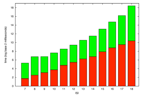
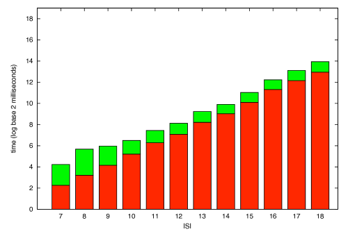
Figure 3: comparison of the computing time (in log base 2 seconds) demanded by the UCS (3) and UBB (3) on the simulated data showed in Table 1. The red bars represent time spent on computation of the cost function, while the green bars are the time spent in the remaining actions of each algorithm. The UCS algorithm always expends more computational time in tasks that does not involve calculating the cost function; on the other hand, the opposite phenomenon occurs with the UBB.

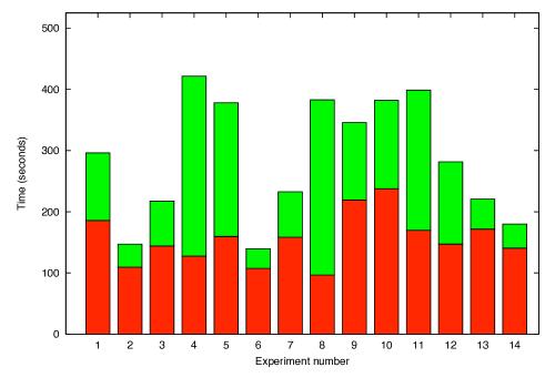
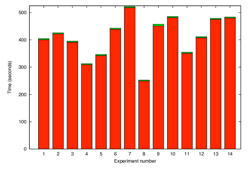
Figure 4: comparison of the computing time (in seconds) demanded by the UCS (4) and UBB (4) on W-operator design showed in Table 2. The red bars represent time spent on computation of the cost function, while the green bars are the time spent in the remaining actions of each algorithm. The UCS algorithm often demands a smaller computational time for the whole feature selection procedure of each W-operator, but it always expends more computational time that does not involve calculating the cost function.

To investigate the facts showed in Figures 3 and 4, we did an analysis of the UCS algorithm dynamics. We executed the UCS on one hundred different instances of the same size. For each instance, we stored the number of times an execution calls the DFS subroutine (i.e., a new depth-first search on the current search space) and the number of times an execution calls either Minimal-Element or Maximal-Element (i.e., returns a new element that might belong to the current search space). Finally, we calculated the averages of calls of DFS and calls of Minimal-Element or Maximal-Element for the hundred instances. In Figures 5 and 5, we present graphics of this ratio in function of the experiment label in, respectively, the optimal and suboptimal-search experiments. These graphics show how many times UCS calls either Minimal-Element or Maximal-Element subroutines until it receives a new element of the current search space, which is a necessary condition to call the DFS subroutine. As the size of the instance increases, UCS needed to perform more calls of the Minimal-Element or Maximal-Element subroutines until it received a new element of the search space. In both graphics, as the size of instance increases, the distance between the green line (calls of Minimal-Element or Maximal-Element) and the orange line (calls of DFS) also increases. For instance, in Figure 5, for instances of size $5$, on the average more than $18\%$ of the iterations find a new element of the current search space; on the other hand, for instances of size $18$, on the average less than $2\%$ of the iterations find a new element of current search space. These graphics show that the search for a new element of the search space is a process that contributes to the high percentage of the green bars on the histogram showed in Figure 4.

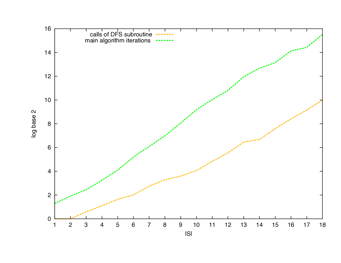
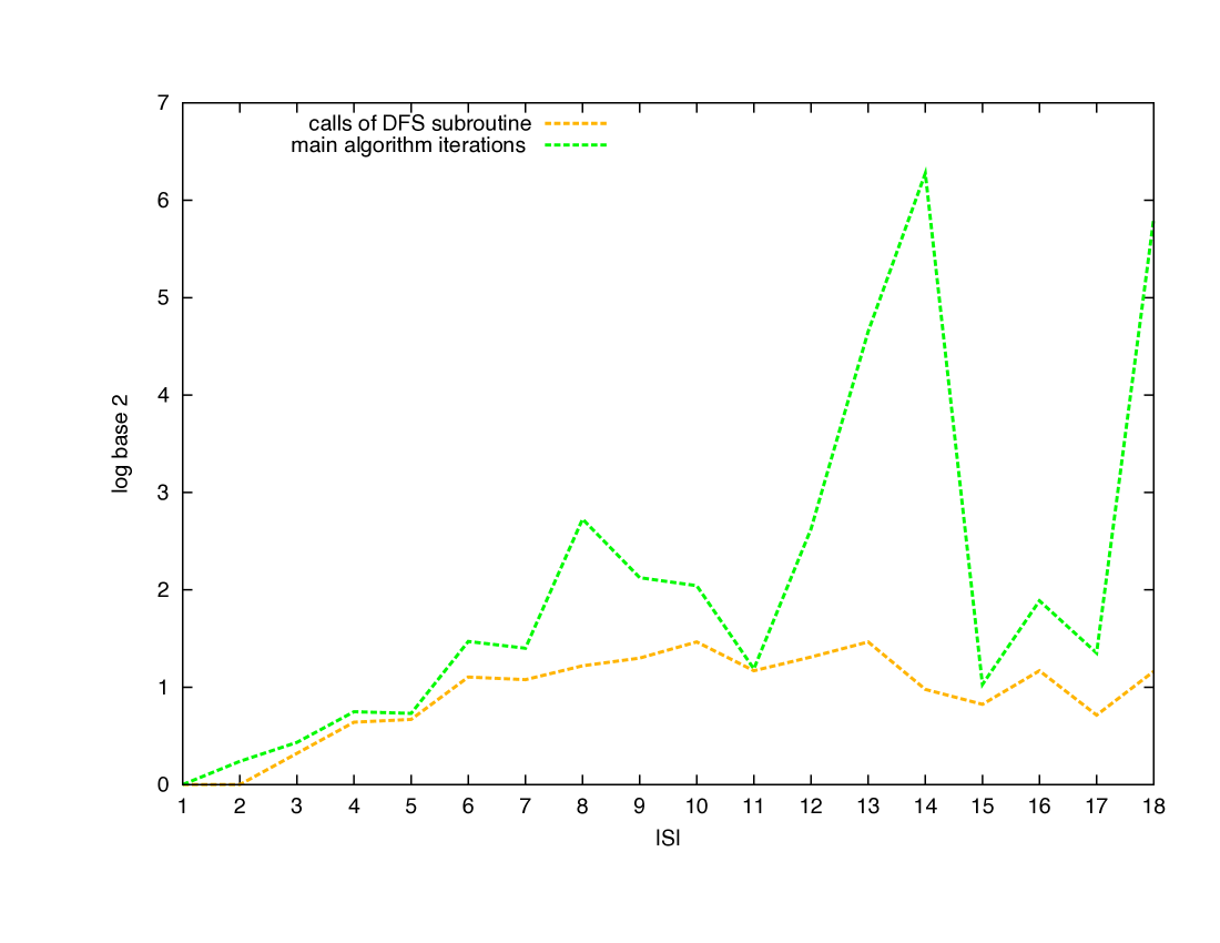
Figure 5: comparison between the number of times the DFS subroutine is called (orange line) and the number of iterations of the main algorithm (green line), during the execution of the UCS algorithm on instances of different sizes. Figures 5 and 5 were produced with the same output used to produce, respectively, Tables 1 (i.e., optimal search on simulated data) and 4 (i.e., heuristic search on simulated data).

One property that was empirically observed in Tables 4 and 6 is that the velocity of convergence of the UCS is much greater than the ones of UBB and SFFS. This property has potential for the design of better optimal-search algorithms, though it has no impact on the complexity analysis of the UCS algorithm.

5 Conclusion

Aiming to solve the U-curve problem, Ris et al. (2010) introduced the U-Curve algorithm. U-Curve is based in the Boolean lattice structure of the search space. The principles of the algorithm are: (i) if the current search space is not empty, then it pushes in a stack an element $M$; otherwise, it stops; (ii) it selects the top of the stack $M$; if there is an element $N$ adjacent to $M$ such that $c(N)\leq c(M)$, then $N$ is pushed in the stack; otherwise, it pops $M$ and uses it to prune the current search space; (iii) if the stack is not empty, then it returns to step (ii); otherwise, it returns to step (i). We demonstrated that this algorithm has a pruning error that leads to suboptimal solutions; the error was pointed out in Figure 1, through a simulation of the algorithm.

This article introduced a new algorithm, the U-Curve-Search (UCS), which is actually optimal to solve the U-curve problem. UCS keeps the general structure of U-Curve, but changes the step (ii): it stores in the head of a linked list elements adjacent to $M$ in the current search space, until it either finds an element $N$ such that $c(N)\leq c(M)$ (i.e., it reaches the depth-first search criterion) or explores all adjacent elements. Moreover, it uses $M$ to prune the current search space only if it is achieved some sufficient conditions to do so without the risk of losing global minima. UCS brings some important improvements: (1) the depth-first search criterion avoids to keep in the memory too many elements, thus providing a better control of the algorithm memory usage; (2) once it achieves a deepest element, it performs less pruning, but very effective ones. The general idea of UCS was showed through a simulation presented in Figure 2.

It was performed a diagnosis of the quality of the UCS algorithm through experiments on simulated and real data. On the one hand, UCS expends too much computational time looking for a new element in the search space, which contributes to the computational time expend in a whole execution of the algorithm. This fact was showed in Figures 5 and 5. On the other hand, the UCS pruning procedures are effective. This fact was suggested by Table 4, which shows that UCS converges relatively fast, and by Figures 3 and 4, which show that UCS computes few nodes while it covers a large subset of the search space.

A comparison between UCS, UBB and SFFS was also made through experiments on simulated and real data. UCS had a better performance in the exploration of the search space than UBB, generally demanding much less computation of the cost function to find an optimal solution. Besides, it often demanded less computational time to find optimal solutions in real data experiments. These facts were showed in Tables 1 and 2 and discussed in Section 4. In the suboptimal-search experiments, UCS had a better performance than the other algorithms, finding more frequently a best solution. Moreover, the velocity of convergence of the UCS is much greater than the ones of UBB and SFFS. These facts were empirically observed by Tables 4 and 6. UBB demanded less computational time than UCS in simulated data experiments, in which the computation of the cost function is inexpensive. This fact was showed in Figure 3. However, Figures 5 and 5 suggest that the difference between algorithms is explained by the UCS inefficient search for an element of the search space.

Future improvements of the UCS algorithm might include: implementation of a more efficient way to find an element of the search space; the development of a new DFS, in which it is processed multiple DFS procedures, which might permit a more homogenous exploration of the search space and thus increasing of the pruning efficiency; build of parallelized versions of the algorithm. Finally, another line of future works would be the definition of subspaces of large Boolean lattices, for instance, delimiting the search space by a collection of intervals, or defining parametrized constraints.

6 Acknowledgments

This work was supported by CNPq scholarship $142039/2007-1$ and FAPESP project $08/51273-9$ (Marcelo da Silva Reis), by CNPq grant $306442/2011-6$ and FAPESP Pronex $2011/50761-2$ (Junior Barrera), and by CNPq grant $302736/2010-7$ (Carlos Eduardo Ferreira).

References

- Barrera et al. (2007) Barrera, J., Cesar-Jr, R., Martins-Jr, D., Vêncio, R., Merino, E., Yamamoto, M., Leonardi, F., Pereira, C., & Portillo, H. (2007). Constructing probabilistic genetic networks of Plasmodium falciparum from dynamical expression signals of the intraerythrocytic development cycle. Methods of Microarray Data Analysis V, (pp. 11–26).
- Barrera et al. (2000) Barrera, J., Terada, R., Hirata-Jr., R., & Hirata, N. (2000). Automatic programming of morphological machines by PAC learning. Fundamenta Informaticae, (pp. 229–258).
- Cormen et al. (2001) Cormen, T., Leiserson, C., Rivest, R., & Stein, C. (2001). Introduction to Algorithms. Cambridge, MA, USA: MIT Press.
- Jain & Mao (2000) Jain, A., & Mao, R. (2000). Statistical pattern recognition: a review. IEEE Transactions on Pattern Analysis and Machine Intelligence, 22, 4–37.
- Kittler (1978) Kittler, J. (1978). Feature set search algorithms. Pattern Recognition and Signal Processing, (pp. 41–60).
- Kudo & Sklansky (2000) Kudo, M., & Sklansky, J. (2000). Comparison of algorithms that select features for pattern classifiers. Pattern Recognition, 33, 25–41.
- Lin (1991) Lin, J. (1991). Divergence measures based on the Shannon entropy. IEEE Transactions on Information Theory, 37, 145–151.
- Marill & Green (1963) Marill, T., & Green, D. (1963). On the effectiveness of receptors in recognition systems. IEEE Transactions on Information Theory, 9, 11–17.
- Martins-Jr et al. (2006) Martins-Jr, D., Cesar-Jr, R., & Barrera, J. (2006). W-operator window design by minimization of mean conditional entropy. Pattern Analysis and Applications, 9, 139–153.
- Meiri & Zahavi (2006) Meiri, R., & Zahavi, J. (2006). Using simulated annealing to optimize the feature selection problem in marketing applications. European Journal of Operational Research, 171, 842–858.
- Nakariyakul & Casasent (2009) Nakariyakul, S., & Casasent, D. (2009). An improvement on floating search algorithms for feature subset selection. Pattern Recognition, 42, 1932–1940.
- Narendra & Fukunaga (1977) Narendra, P., & Fukunaga, K. (1977). A branch and bound algorithm for feature subset selection. IEEE Transactions on Computers, 100, 917–922.
- Piramuthu (2004) Piramuthu, S. (2004). Evaluating feature selection methods for learning in data mining applications. European Journal of Operational Research, 156, 483–494.
- Pudil et al. (1994) Pudil, P., Novovicová, J., & Kittler, J. (1994). Floating search methods in feature selection. Pattern Recognition Letters, 15, 1119–1125.
- Reis (2012) Reis, M. (2012). Minimization of decomposable in U-shaped curves functions defined on poset chains – algorithms and applications. Ph.D. thesis Institute of Mathematics and Statistics, University of São Paulo, Brazil. (in Portuguese).
- Ris et al. (2010) Ris, M., Barrera, J., & Martins-Jr, D. (2010). U-curve: A branch-and-bound optimization algorithm for U-shaped cost functions on Boolean lattices applied to the feature selection problem. Pattern Recognition, 43, 557–568.
- Schrijver (2000) Schrijver, A. (2000). A combinatorial algorithm minimizing submodular functions in strongly polynomial time. Journal of Combinatorial Theory, Series B, 80, 346–355.
- Somol et al. (1999) Somol, P., Pudil, P., Novovicová, J. et al. (1999). Adaptive floating search methods in feature selection. Pattern Recognition Letters, 20, 1157–1163.
- Theodoridis & Koutroumbas (2006) Theodoridis, S., & Koutroumbas, K. (2006). Pattern Recognition. Elsevier, Academic Press, Amsterdam, New York.
- Unler & Murat (2010) Unler, A., & Murat, A. (2010). A discrete particle swarm optimization method for feature selection in binary classification problems. European Journal of Operational Research, 206, 528–539.
- Whitney (1971) Whitney, A. W. (1971). A direct method of nonparametric measurement selection. IEEE Transactions on Computers, 20, 1100–1103.