Rapid Change of Field Line Connectivity and Reconnection in Stochastic Magnetic Fields

Abstract

Magnetic fields without a direction of continuous symmetry have the generic feature that neighboring field lines exponentiate away from each other and become stochastic, hence the ideal constraint of preserving magnetic field line connectivity becomes exponentially sensitive to small deviations from ideal Ohm’s law. The idea of breaking field line connectivity by stochasticity as a mechanism for fast reconnection is tested with numerical simulations based on reduced magnetohydrodynamics equations with a strong guide field line-tied to two perfectly conducting end plates. Starting from an ideally stable force-free equilibrium, the system is allowed to undergo resistive relaxation. Two distinct phases are found in the process of resistive relaxation. During the quasi-static phase, rapid change of field line connectivity and strong induced flow are found in regions of high field line exponentiation. However, although the field line connectivity of individual field lines can change rapidly, the overall pattern of field line mapping appears to deform gradually. From this perspective, field line exponentiation appears to cause enhanced diffusion rather than reconnection. In some cases, resistive quasi-static evolution can cause the ideally stable initial equilibrium to cross a stability threshold, leading to formation of intense current filaments and rapid change of field line mapping into a qualitatively different pattern. It is in this onset phase that the change of field line connectivity is more appropriately designated as magnetic reconnection. Our results show that rapid change of field line connectivity appears to be a necessary, but not a sufficient condition for fast reconnection.

1 Introduction

Magnetic reconnection is a fundamental process in astrophysical, space, and laboratory plasmas, which can change the topology of magnetic field lines, release magnetic energy, and accelerate electrons and ions (Biskamp, 2000; Priest & Forbes, 2000; Zweibel & Yamada, 2009; Yamada et al., 2010). It is generally believed that magnetic reconnection is the underlying mechanism that powers explosive events such as solar flares, coronal mass ejections, geomagnetic substorms, and sawtooth crashes in fusion devices.

Much of the literature on magnetic reconnection focuses on two-dimensional (2D) problems, i.e. when the whole reconnection process only depends on two spatial coordinates under a proper coordinate system, for reasons of analytic and numerical simplicity. At this time, theories of 2D magnetic reconnection are highly developed and fairly well-understood. Magnetic reconnection in 2D is known to take place at an X-point (or X-line), where magnetic field line separatrices intersect; across separatrices the field line mapping is discontinuous. As a magnetic field line is carried across a separatrix by plasma flow, the velocity field that preserves magnetic field line connectivity (i.e. the velocity field carries a field line at one time to another field line at a later time) diverges at the X-point (Priest et al., 2003); that is, the field line is cut and rejoined with another field line at the X-point.

Real world magnetic reconnection of course takes place in three dimensions (3D). Compared with 2D problems, magnetic reconnection in 3D is much less well-understood [see, e.g. Pontin (2011) for a recent review, and the references therein.] Even the concept of magnetic reconnection can sometimes become ambiguous, especially in the absence of magnetic null points or closed magnetic field lines. In these situations, all magnetic field lines are topologically equivalent, and a continuous velocity field that preserves magnetic field line connectivity can always be defined (Greene, 1993). Where, then, does magnetic reconnection take place? Quasi-separatrix layers (QSLs), defined as regions where the field line mapping has large gradient (Priest & Démoulin, 1995; Démoulin et al., 1996; Titov, 2007), have been suggested as likely locations for reconnection to take place. Although field line velocity can always be defined in a 3D magnetic field without null points or closed field lines, the field line velocity can differ significantly from the plasma velocity around QSLs. The concept of QSLs have been widely employed in analyzing 3D magnetic reconnection in recent numerical simulations and laboratory experiments (Lawrence & Gekelman, 2009; Richardson & Finn, 2012; Gekelman et al., 2014; Finn et al., 2014).

In a magnetic field with no ignorable coordinates, magnetic field lines generically exponentiate apart from each other and become stochastic. Such a generic condition usually occurs in space and astrophysical plasmas as well as in a number of contexts in laboratory plasmas (including toroidal fusion plasmas) in the presence of multiple tearing modes. Also, global simulation codes for space weather studies often exhibit magnetic turbulence (at fluid as well as kinetic levels) which produces field-line exponentiation. That means that if we follow two field lines initially separated by an infinitesimal distance $\delta r(0)$, in most cases the separation grows exponentially as $\delta r(\ell)=e^{\sigma(\ell)}\delta r(0)$, where $\ell$ is the distance along the field line, and $\sigma(\ell)$ is an overall (but in general not monotonically) increasing function over distance. This fact is analogous to the well-known butterfly effect in the theory of deterministic dynamical systems as a sensitive dependence on initial conditions. Boozer (2012a, b, 2013) has recently argued that under the condition of large field line exponentiation, an exponentially small non-ideal effect will completely scramble the field line mapping, and potentially lead to fast reconnection. Although the notion of large field line exponentiation shares common ground with the concept of QSLs, an important difference is that the condition for neighboring field line exponentiation is valid essentially for all field lines, therefore regions of large field line exponentiation do not necessarily concentrate in layers and can even be volume filling.

The motivation of this study is to test this scenario proposed by Boozer with numerical experiments as clean as possible. To this end we consider relaxation of force-free equilibria in a region bounded by two conducting plates under the effect of a finite but small resistivity. Without resistivity, the field line mapping from one end to another is preserved. With a finite resistivity, the field line mapping evolves as time proceeds. We find that in general the field line connectivity changes rapidly in regions with large neighboring field line exponentiation. However, not all rapid changes of field line connectivity are associated with what is usually regarded as reconnection. We find two distinct phases of evolution — one is the quasi-static phase and the other the onset phase. The onset phase is triggered by some magnetohydrodynamic (MHD) instability. We find that change of field line connectivity during the quasi-static phase is more properly attributed to enhanced magnetic diffusion, whereas typical hallmarks of reconnection are found during the onset phase.

This paper is organized as follows. In Section 2 we introduce the reduced magnetohydrodynamics (RMHD) model and simulation setup. In Section 3, we introduce the details of diagnostics used to analyze the simulations. Section 4 presents two sets of simulations. The first set is governed by resistive quasi-static evolution, and the second set features the onset phase. Section 5 discusses important issues that arise from the simulation results, including the governing equations for resistive quasi-static evolution, the cause of the onset phase, and some measures to quantify the distinction between the two phases. Finally, we summarize the key findings and conclude in Section 6. In Appendix A, we explain the procedure of constructing the initial RMHD force-free equilibrium in detail, and make comparison with the corresponding problem in full MHD.

2 Model and Simulation Setup

We employ the standard reduced magnetohydrodynamics (RMHD) model (Kadomtsev & Pogutse, 1974; Strauss, 1976; van Ballegooijen, 1985), which is valid in the presence of a strong uniform guide field, under the assumption that spatial length scales are much longer along the direction of the guide field than in directions perpendicular to the guide field. The governing equations can be written as:

$$\partial_{t}\Omega+[\phi,\Omega]=\partial_{z}J+[A,J]+\nu\nabla_{\perp}^{2}\Omega-\lambda\Omega,$$ (1)

$$\partial_{t}A+[\phi,A]=\partial_{z}\phi+\eta\nabla_{\perp}^{2}A.$$ (2)

Here we assume the guide field to be along the $z$ direction, with the strength normalized to unity. The magnetic field $\mathbf{B}$ and the plasma velocity $\mathbf{u}$ are expressed in terms of the flux function $A$ and the stream function $\phi$ through the relations $\mathbf{B}=\mathbf{\hat{z}}+\nabla_{\perp}A\times\mathbf{\hat{z}}$ and $\mathbf{u}=\nabla_{\perp}\phi\times\mathbf{\hat{z}}$; and $\Omega\equiv-\nabla_{\perp}^{2}\phi$ and $J\equiv-\nabla_{\perp}^{2}A$ are vorticity and electric current along the $z$ direction, respectively. The Poisson bracket is defined as $\left[f,g\right]=\partial_{y}f\partial_{x}g-\partial_{x}f\partial_{y}g$. Dissipations are introduced by including resistivity $\eta$, viscosity $\nu$, and a friction coefficient $\lambda$. We assume that the system is bounded in the $z$ direction by two conducting end plates at $z=0$ and $z=L$, and is a $1\times 1$ box with doubly periodic boundary condition in the $x-y$ plane. RMHD models are often used in analytic and numerical studies of Parker’s coronal heating model (van Ballegooijen, 1985; Strauss & Otani, 1988; Longcope & Strauss, 1994a; Longcope & Sudan, 1994; Ng & Bhattacharjee, 1998; Dmitruk & Gómez, 1999; Dmitruk et al., 2003; Rappazzo et al., 2007, 2008; Ng & Bhattacharjee, 2008; Ng et al., 2012; Rappazzo & Parker, 2013). However, unlike simulations of Parker’s model, here we impose no boundary flow, i.e. the boundary conditions are $\phi=0$ at $z=0$ and $z=L$. The governing equations are solved with a reduced version of the compressible MHD code DEBS (Schnack et al., 1986). The $x-y$ plane is discretized with a pseudospectral method, and the $z$ direction is discretized with a finite difference method, where $\phi$ and $A$ reside on staggered grids. The timestepping is carried out with a semi-implicit, predictor-corrector leapfrog method, where $\phi$ and $A$ are staggered in time as well.

In this model, resistivity provides the mechanism that breaks the ideal constraint of frozen field lines, whereas viscosity and friction are introduced to damp Alfvén waves that will be generated when the system is not in force equilibrium, e.g. due to reconnection. Undamped Alfvén waves bouncing back and forth between the two conducting end plates may lead to fine structures through distortion of wave packets and phase mixing, especially in regions where the magnetic field is highly sheared (Similon & Sudan, 1989). Although this phenomenon can be very important in wave dissipation and heating, it further complicates the problem and may lead to numerical difficulties. For these reasons, we opt for damping out Alfvén waves in order to to make the simulations as clean as possible.

A force-free equilibrium in RMHD satisfies the condition $\partial_{z}J+\left[A,J\right]=\mathbf{B}\cdot\nabla J=0.$ Formally, this equation is isomorphic to the 2D Euler’s equation of incompressible fluid, if we identify $z$ with a time variable, and $A$ with the stream function. Therefore, if $A$ is specified on a $x-y$ plane, we can construct the corresponding force-free equilibrium by integrating $\mathbf{B}\cdot\nabla J=0$ along $z$ (see Appendix A for details of numerical implementation). In our simulations, we construct the initial conditions by specifying the flux function at the mid-plane $A|_{z=L/2}$ as a superposition of Fourier harmonics

$$A|_{z=L/2}=\sum_{m,n}a_{mn}\exp(i\pi(mx+ny)),$$ (3)

where the coefficients $a_{mn}$ are complex random numbers whose magnitudes $\left|a_{mn}\right|$ on average scale as $\left|a_{mn}\right|\sim\left(m^{2}+n^{2}\right)^{-2}$. Only mode numbers $m$, $n$ within the range $2\leq\sqrt{m^{2}+n^{2}}\leq 5$ are used. In addition, the coefficients $a_{mn}$ must satisfy the reality condition $a_{mn}=a_{-m-n}^{*}$. Because Euler’s equation conserves energy, the equilibrium satisfies

$$\frac{d}{dz}\int\frac{1}{2}B_{\perp}^{2}dxdy=0,$$ (4)

where $\mathbf{B}_{\perp}=\nabla_{\perp}A\times\mathbf{\hat{z}}$ is the magnetic field component on the $x-y$ plane.

In this study, first a set of Fourier coefficients $a_{mn}$ are randomly chosen. Subsequently, they are rescaled to a given $E_{\perp}\equiv\int\frac{1}{2}B_{\perp}^{2}dxdy$, which is used as a free parameter to prescribe the initial equilibrium. We set the system length to a fixed value $L=10$. This value of system length is arbitrary and does not affect the results, because the RMHD model is scale-invariant. That is, if $\phi(\mathbf{x_{\perp}},z,t)$ and $A(\mathbf{x_{\perp}},z,t)$ form a solution of RMHD with dissipation coefficients $\nu$, $\eta$, and $\lambda$, then for an arbitrary rescale factor $\zeta$, the rescaled solutions $\phi\to\zeta\phi(\mathbf{x_{\perp}},\zeta z,\zeta t)$ and $A\to\zeta A(\mathbf{x_{\perp}},\zeta z,\zeta t)$ satisfy RMHD with dissipation coefficients $\nu\to\zeta\nu$, $\eta\to\zeta\eta$, and $\lambda\to\zeta\lambda$. Therefore, a solution with respect to a given system length $L$ can always be rescaled to another solution with a system length $L^{\prime}=\zeta L$.

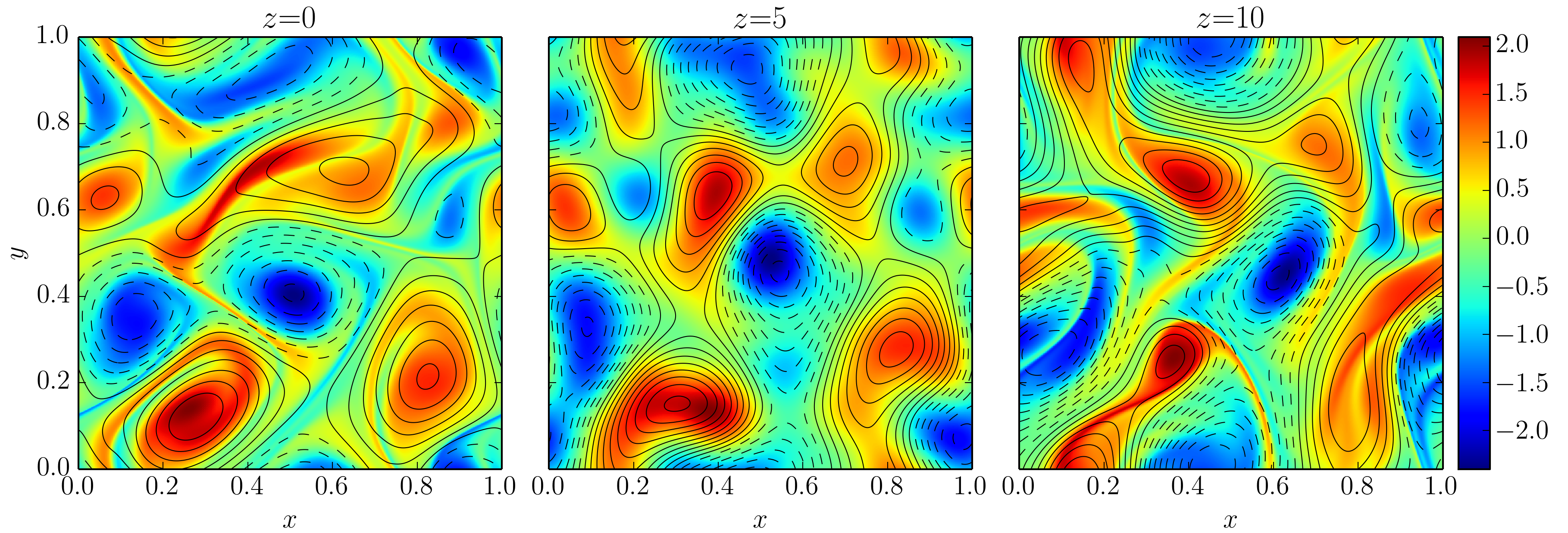
Figure 1: Slices of initial current density $J$ profile, overlaid with contours of the flux function $A$, on $x-y$ planes at $z=0$, $z=5$, and $z=10$, for the case $E_{\perp}=1.4\times 10^{-3}$.

Figure 1 show slices of initial current density profile, overlaid with contours of the flux function $A$, on $x-y$ planes at $z=0$, $z=5$, and $z=10$, for the case $E_{\perp}=1.4\times 10^{-3}$. Because Equation (3) only contains long wavelength Fourier harmonics, the current density $J$ is smooth at $z=5$. However, as we integrate $\mathbf{B}\cdot\nabla J=0$ along both $\pm z$ directions, constant-$J$ contours become increasingly stretched and develop fine structures due to field line exponentiation. If the neighboring field lines exponentiate by a factor of $e^{\sigma}$, $\left|\nabla J\right|$ can be amplified by a factor up to $e^{\sigma}$. In the present case, although $J$ is of the order unity in the whole domain, $\left|\nabla J\right|$ clearly becomes large at $z=0$ and $z=10$.

Once the initial equilibrium is constructed, we study resistive relaxation under different values of resistivity $\eta$. We fix the viscosity $\nu=10^{-6}$ and the friction coefficient $\lambda=0.1$. Through numerical experiments, we find that these values are sufficient to effectively damp out Alfvén wave in a few Alfvén transit times.

3 Diagnostics

Neighboring field line exponentiation is characterized by the exponent $\sigma$, which can be calculated by simultaneously integrating the equation for field line

$$\frac{d\mathbf{x}_{\perp}}{dz}=\mathbf{B_{\perp}}$$ (5)

and the equation for infinitesimal separation $\delta\mathbf{x}_{\perp}$ between neighboring field lines:

$$\frac{d\delta\mathbf{x}_{\perp}}{dz}=\delta\mathbf{x}_{\perp}\cdot\nabla_{\perp}\mathbf{B}_{\perp}.$$ (6)

In terms of the flux function $A$, Equation (5) can be written as

$$\frac{d}{dz}\left[\begin{array}[]{c}x\\ y\end{array}\right]=\left[\begin{array}[]{c}\partial_{y}A\\ -\partial_{x}A\end{array}\right].$$ (7)

Hence, the flux function $A$ is the Hamiltonian for field lines, if we identify $z$ with a time variable. Equation (6) can be written in matrix form as:

$$\frac{d}{dz}\left[\begin{array}[]{c}\delta x\\ \delta y\end{array}\right]=\left[\begin{array}[]{cc}\partial_{x}B_{x}&\partial_{y}B_{x}\\ \partial_{x}B_{y}&\partial_{y}B_{y}\end{array}\right]\left[\begin{array}[]{c}\delta x\\ \delta y\end{array}\right]\equiv M(z)\left[\begin{array}[]{c}\delta x\\ \delta y\end{array}\right],$$ (8)

which can be formally solved as

$$\left[\begin{array}[]{c}\delta x\\ \delta y\end{array}\right]=\exp\left(\int_{0}^{z}M(z^{\prime})dz^{\prime}\right)\left[\begin{array}[]{c}\delta x\\ \delta y\end{array}\right]_{z=0}\equiv N(z)\left[\begin{array}[]{c}\delta x\\ \delta y\end{array}\right]_{z=0},$$ (9)

where the integration is carried out along the field line. However, direct numerical calculation of $\exp\left(\int_{0}^{z}M(z^{\prime})dz^{\prime}\right)$ is prone to numerical instability. Therefore, in practice the matrix $N(z)$ is calculated by integrating the equation

$$\frac{dN}{dz}=MN,$$ (10)

with the initial condition

$$N|_{z=0}=\left[\begin{array}[]{cc}1&0\\ 0&1\end{array}\right].$$ (11)

Because the field line mapping in RMHD preserves area, the singular value decomposition (SVD) (Trefethen & Bau, 1997) of $N(z)$ is of the form

$$N(z)=U(z)\left[\begin{array}[]{cc}e^{\sigma(z)}&0\\ 0&e^{-\sigma(z)}\end{array}\right]V^{T}(z),$$ (12)

where both $U(z)$ and $V(z)$ are unitary matrices. The factor $e^{\sigma(z)}$ gives the maximum exponentiation we could have for two neighboring field lines. A geometrical interpretation of the exponent $\sigma(z)$ is that, if we follow a thin flux tube starting with a circular cross section of radius $\delta r$ at $z=0$, the cross section becomes an ellipse at $z>0$, with $\delta r_{max}=e^{\sigma(z)}\delta r$ and $\delta r_{min}=e^{-\sigma(z)}\delta r$ as the major and minor radii, respectively. This interpretation bears resemblance to the squashing factor $Q$ often employed in the definition of QSLs (Titov, 2007), which is defined as

$$Q=\frac{\delta r_{max}}{\delta r_{min}}+\frac{\delta r_{min}}{\delta r_{max}}$$ (13)

measured at the top plate. In the limit $\sigma(L)\gg 1$, the exponent $\sigma(L)$ is related to the squashing factor $Q$ by the relation $Q\simeq e^{2\sigma(L)}$. However, note that neighboring field line exponentiation is a more general concept, in the sense that the squashing factor $Q$ depends only on the field line mapping from one end plate to another, but not on the field line separation that occurs in the region between the two plates.

In this study, individual field lines are treated as fundamental entities, labeled by their footpoints at the bottom plate. Along each field line, we calculate the following quantities:

1. The maximum value of the exponent $\sigma_{max}\equiv\underset{0\leq z\leq L}{\max}\sigma(z)$. This provides information of the locations where the neighboring field lines strongly exponentiate apart.

2. Drift of footpoints of magnetic field lines at the top plate between two consecutive snapshots separated by one Alfvén transit time ($=10$ in the simulation) when the footpoints at the bottom plate is held fixed. Without non-ideal effects, the footpoint drift should be identically zero.

3. Kinetic energy density $\int_{0}^{L}\frac{1}{2}\left|\nabla_{\perp}\phi\right|^{2}dz$. This provides information of where the energy conversion from magnetic field to kinetic energy occurs.

4. Parallel electric voltage $\int\mathbf{E}\cdot d\mathbf{l}=\int_{0}^{L}\eta Jdz$. This is often employed as a proxy for reconnection rate in 3D (Schindler et al., 1988; Hesse & Schindler, 1988; Hesse et al., 2005).

By using field lines as the fundamental entities, we effectively reduce the 3D information to 2D. We typically trace $400\times 400$ field lines arranged in a uniform array at the bottom plate in each snapshot.

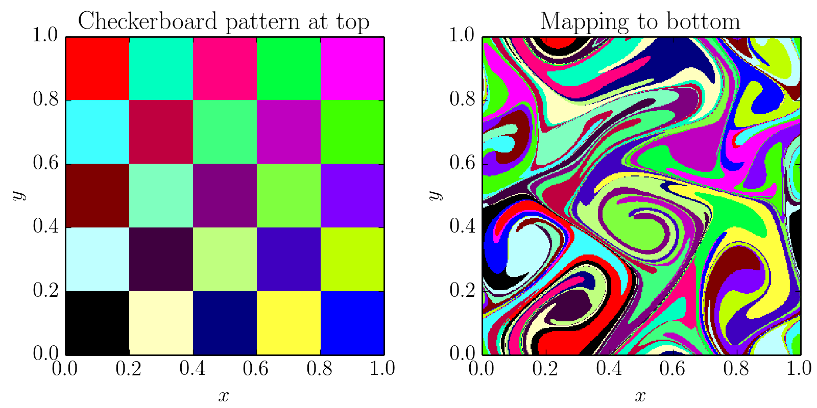
Figure 2: Visualization of footpoint mapping between two end plates, for the initial condition with $E_{\perp}=1.4\times 10^{-3}$. Left panel shows a $5\times 5$ checkerboard pattern at the top plate; the right panel shows the pattern at the bottom plate, when the checkerboard pattern is pulled back by the footpoint mapping.

We visualize the field line mapping between two plates as follows. First a checkerboard pattern is laid out at the top plate, which is then pulled back to the bottom plate by the field line mapping. The resulting pattern at the bottom plate gives a visualization of the field line mapping. Figure 2 shows an example of such visualization for the initial condition with $E_{\perp}=1.4\times 10^{-3}$. Here we have made use of the doubly periodic boundary condition in defining field line mapping between the two plates, such that the top plate of the simulation box is exactly mapped to the bottom plate. As a result of neighboring field line exponentiation, the checkerboard pattern becomes highly distorted when pulled back to the bottom plate.

4 Simulation Results

Two sets of simulations have been carried out for this study, with $E_{\perp}=1.25\times 10^{-3}$ and $E_{\perp}=1.4\times 10^{-3}$, respectively. Both initial conditions are ideally stable; i.e. they remain unchanged for a long time when $\eta$ is set to zero. The two initial conditions are subjected to resistive relaxation with different $\eta$. Parameters of the reported simulations in this paper are listed in Table 1. Convergence test has been carried out for selected runs. Specifically, Run B2 and Run B3 have been tested with a lower resolution $512^{3}$, and the results are essentially the same as the higher resolution runs presented in the paper.

Run	$E_{\perp}$	$\eta$	Resolution
A1	$1.25\times 10^{-3}$	$10^{-5}$	$512^{3}$
A2	$1.25\times 10^{-3}$	$5\times 10^{-6}$	$512^{3}$
A3	$1.25\times 10^{-3}$	$2.5\times 10^{-6}$	$512^{3}$
A4	$1.25\times 10^{-3}$	$10^{-6}$	$512^{3}$
B1	$1.4\times 10^{-3}$	$10^{-5}$	$512^{3}$
B2	$1.4\times 10^{-3}$	$5\times 10^{-6}$	$768^{3}$
B3	$1.4\times 10^{-3}$	$2.5\times 10^{-6}$	$768^{3}$

Table 1: Simulation parameters of the Runs reported in this paper. The viscosity $\nu$ and friction coefficient $\lambda$ are kept constant with $\nu=10^{-6}$ and $\lambda=0.1$.

4.1 Case A: $E_{\perp}=1.25\times 10^{-3}$

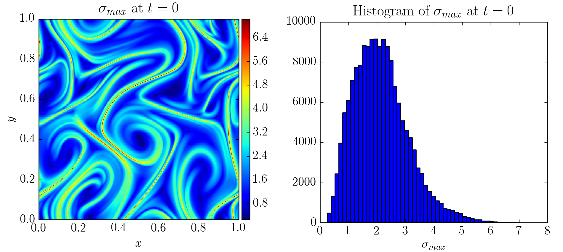
Figure 3: Left panel shows the initial $\sigma_{max}$ profile for Case A with $E_{\perp}=1.25\times 10^{-3}$, labeled by the footpoints of field lines at the bottom plate. Right panel shows the histogram of $\sigma_{max}$.

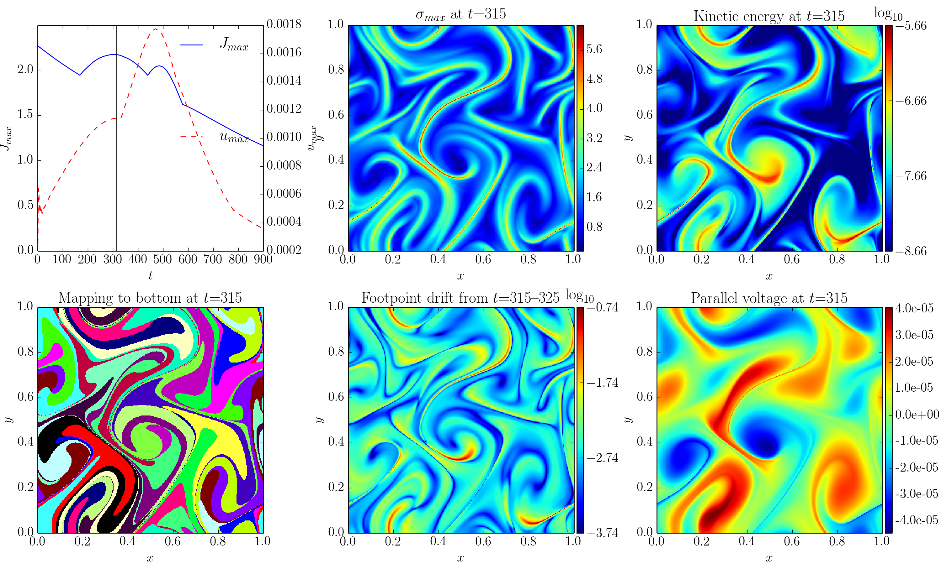
Figure 4: A snapshot at $t=315$ from Run A3. Top left panel shows the time histories of maximum current $J_{max}$ and flow velocity $u_{max}$ of the whole domain, where the vertical line indicates the time the snapshot is taken. The remaining five panels show key diagnostics: field line mapping, and profiles of $\sigma_{max}$, footpoint drift, kinetic energy density, and parallel voltage (movie available online). Note that the kinetic energy density and footpoint drift are colored in logarithmic scales.

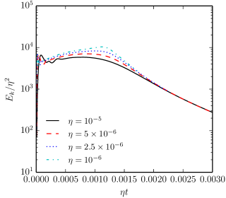
Figure 5: The rescaled total kinetic energy $E_{k}/\eta^{2}$ against the rescaled time $\eta t$ for four different $\eta$ in Case A. The four curves approximately collapse to the same curve, except that there are slight deviations in the middle, when $0.0005\lesssim\eta t\lesssim 0.0015$.

The first set of simulations A1 – A4 start with the initial condition set by $E_{\perp}=1.25\times 10^{-3}$. The initial profile and histogram of $\sigma_{max}$ are shown in Figure 3. As shown in the left panel, regions with high $\sigma_{max}$ typically form layers. The histogram in the right panel shows that for the majority of field lines, $\sigma_{max}$ is around 2. The maximum $\sigma_{max}$ in the whole domain is approximately 7.1.

When the simulation is run with $\eta\neq 0$, the magnetic field decays resistively. Figure 4 shows a snapshot of diagnostics at $t=315$ from Run A3. The top left panel shows the time history of maximum current $J_{max}$ and flow velocity $u_{max}$ within the whole domain, where the vertical line indicates the time the snapshot is taken. The remaining five panels show key diagnostics: field line mapping, and profiles of $\sigma_{max}$, footpoint drift, kinetic energy density, and parallel voltage. All the snapshots from this Run are available online as a movie. From the time histories, we can see that overall $J_{max}$ decays over time, whereas $u_{max}$ gradually increases in the beginning and reaches a peak at $t\simeq 500$, then gradually decays. We also observe that the $\sigma_{max}$ profile is highly correlated with the kinetic energy density and footpoint drift. Usually the kinetic energy density and footpoint drift tend to be high at regions where $\sigma_{max}$ is high. The parallel voltage remains low ($<5\times 10^{-5}$) throughout the simulation and no thin current sheets have formed.

The footpoints of individual field lines in high-$\sigma_{max}$ regions can drift significantly (up to $\simeq 0.3$) within one Alfvén transit time ($=10$ in the simulation unit), assuming that the footpoints at the bottom plate are held fixed. That gives a footpoint drift speed up to $\simeq 0.03$. In comparison, the plasma flow speed only reaches a maximum $\simeq 0.0018$, which is significantly lower than the footpoint speed. The large deviation between plasma flow speed and field line speed suggests possible occurrence of magnetic reconnection. However, at the lower left panel of the movie associated with Figure 4, we do not observe any sudden change in the overall pattern of footpoint mapping, as one would expect from magnetic reconnection. Rather, the initial convoluted field line mapping gradually untwists and becomes simpler, and the dynamics is quiescent and uneventful. Therefore, the rapid footpoint speed here appears to be an artifact caused by magnetic diffusion in the presence of large gradients in the field line mapping, rather than a manifestation of qualitative change in the mapping itself.

Resistive relaxation of this initial condition has been carried out for four different $\eta$. If the dynamics is solely governed by resistive diffusion, we expect that the evolution time scale $\sim 1/\eta$ and flow speed $\sim\eta$. Therefore, if we plot the rescaled total kinetic energy $E_{k}/\eta^{2}$ against the rescaled time $\eta t$, the curves from different runs should collapse to the same curve. Figure 5 shows the rescaled curves for four different $\eta$. And indeed the four curves approximately collapse to the same curve, except that there are slight deviations in the middle, when $0.0005\lesssim\eta t\lesssim 0.0015$. Therefore, we conclude that in this case the dynamics is largely governed by resistive diffusion, rather than reconnection, even if the footpoints of individual field lines can drift rapidly. Because the overall time scale $\sim 1/\eta$, the apparent “drift velocity” of footpoint is expected to scale as $\sim\eta$.

4.2 Case B: $E_{\perp}=1.4\times 10^{-3}$

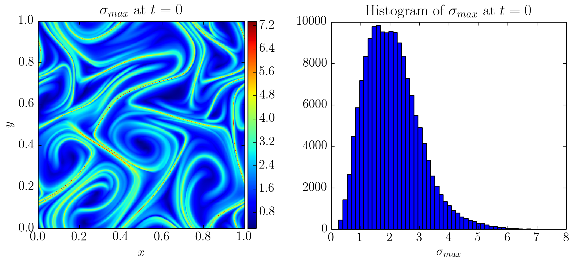
Figure 6: Left panel shows the initial $\sigma_{max}$ profile for Case B with $E_{\perp}=1.4\times 10^{-3}$, labeled by the footpoints of field lines at the bottom plate. Right panel shows the histogram of $\sigma_{max}$.

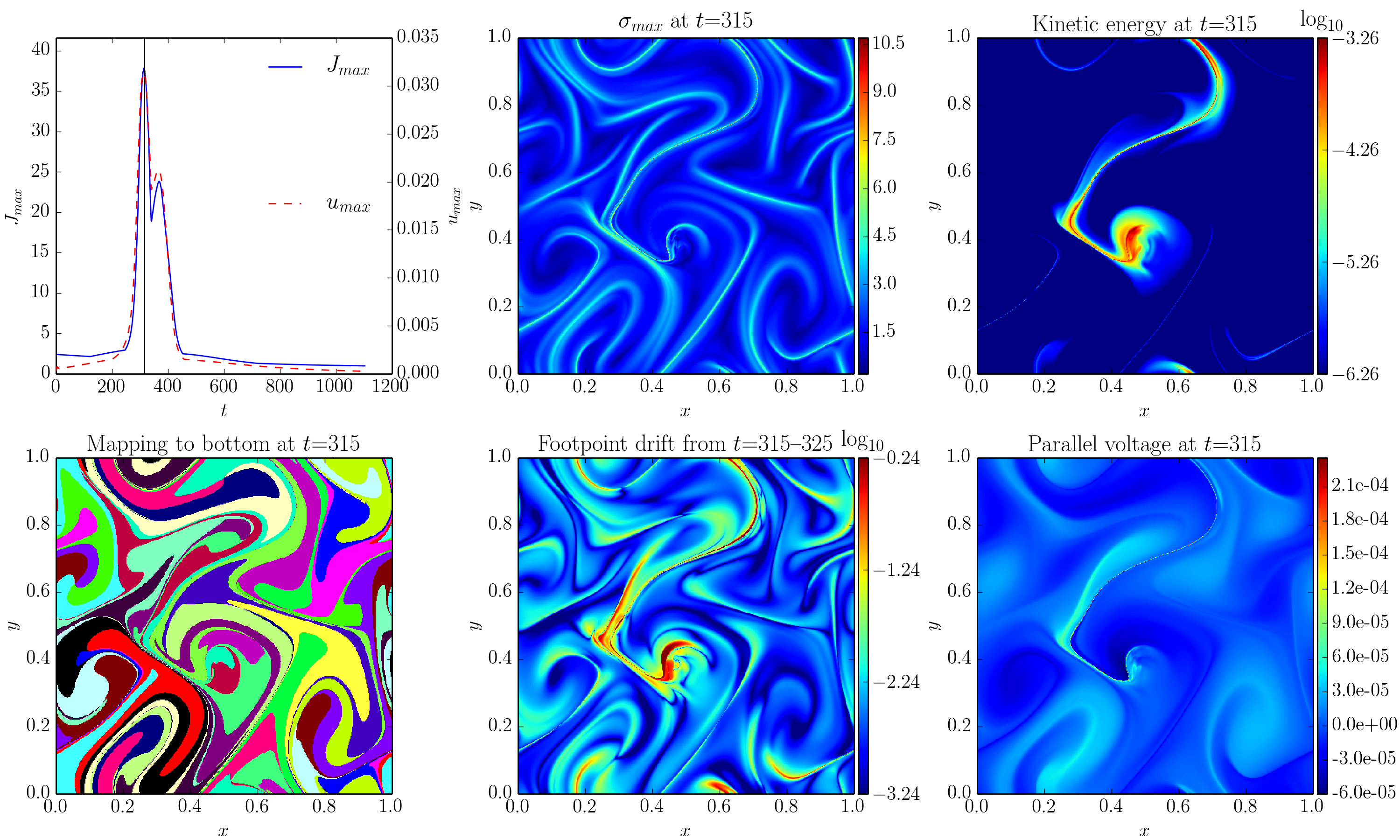
Figure 7: A snapshot at $t=315$ from Run B3. Top left panel shows the time history of maximum current $J_{max}$ and flow velocity $u_{max}$ of the whole domain, where the vertical line indicates the time the snapshot is taken. The remaining five panels show key diagnostics: field line mapping, and profiles of $\sigma_{max}$, footpoint drift, kinetic energy density, and parallel voltage (movie available online). Note that the kinetic energy density and footpoint drift are colored in logarithmic scales.

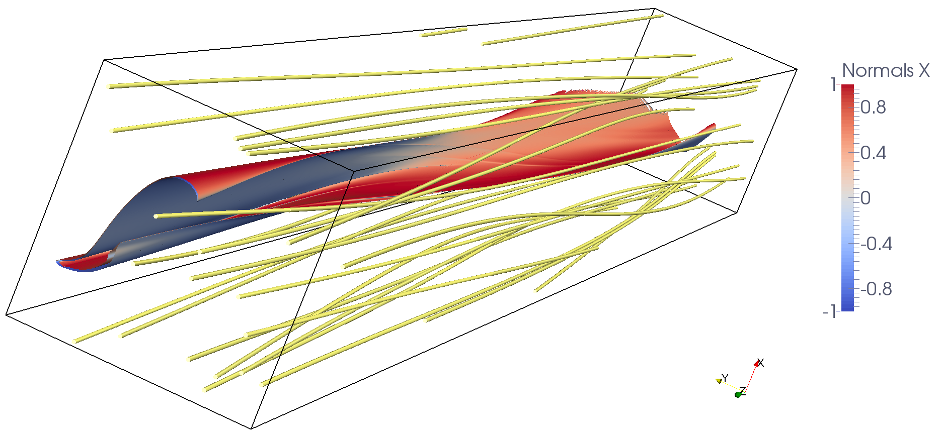
Figure 8: Isosurface of the current density with $J=2$, at $t=315$ when the current intensity peaks. The isosurface is colored according to the $x$-component of the unit normal vector for better visualization. Yellow lines are samples of magnetic field lines.

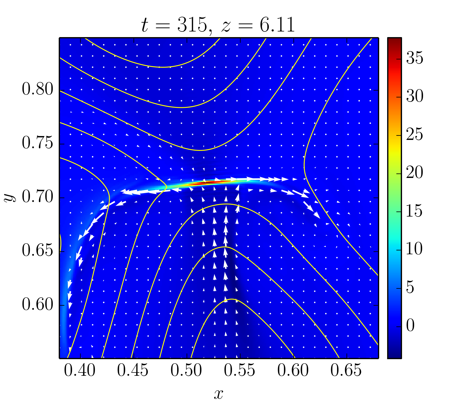
Figure 9: 2D slice of current density (color gradient), plasma flow (white arrows), and contours of flux function $A$ (yellow solid lines) along $z=6.11$, where the current density peaks at $t=315$.

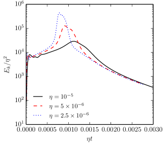
Figure 10: The rescaled total kinetic energy $E_{k}/\eta^{2}$ against the rescaled time $\eta t$ for three different $\eta$ in Case B. The thee curves approximately collapse to the same curve during the early and late quiescent phases. However, they strongly deviate from each other during the “onset” phase in the middle.

The second set of simulations B1 – B3 start with the initial condition set by $E_{\perp}=1.4\times 10^{-3}$. The initial profile and histogram of $\sigma_{max}$ are shown in Figure 6. The $\sigma_{max}$ profile and histogram are qualitatively similar to that of Case A. The maximum $\sigma_{max}$ in the whole domain is approximately 7.4, slightly higher than that of Case A. As we will see, although Case A and Case B do not differ significantly in the initial $\sigma_{max}$ profiles, they lead to very different dynamical behavior at later times.

Figure 7 shows a snapshot at $t=315$ from Run B3, with an accompanying movie available online. From the time histories of $J_{max}$ and $u_{max}$ shown in the upper left panel, we can see that the system relaxes quiescently in the beginning (similar to Case A) until $t\simeq 260$. After that, both $J_{max}$ and $u_{max}$ increase rapidly by an order of magnitude and reach their peak magnitudes at $t\simeq 315$. As can be seen from the kinetic energy density, footpoint drift and parallel voltage profiles in the snapshot at $t=315$, the “onset” occurs in one sigmoid region where $\sigma_{max}$ is large. In this region, the footpoint drift speed reaches a peak value $\simeq 0.06$, the kinetic energy density increases by two orders of magnitude compared to the quiescent phase. The maximum exponent $\sigma_{max}$ increases to a peak value $\simeq 10$ and the parallel voltage increases by a factor of $\simeq 5$ compared to the background voltage before the onset, due to the formation of current filaments in the onset region. After the system has released its magnetic free energy, the evolution becomes quiescent again after $t\simeq 450$. We also note from the accompanying movie that during this “onset” phase the pattern of footpoint mapping undergoes a rapid qualitative change, rather than a gradual deformation as during the quiescent phases.

During the onset phase, a ribbon-like thin current sheet forms, as shown by the $J=2$ isosurface in Figure 8. We also find signatures of magnetic reconnection near the current sheet. Figure 9 shows a 2D slice of current density (color gradient), plasma flow (white arrows), and contours of flux function $A$ (yellow solid lines) at the vicinity of the peak current density. The flux function contours form a X-type geometry near the current sheet, and the plasma flow exhibits the typical inflow and outflow pattern of magnetic reconnection. The reconnection is asymmetric, where the inflow from below is significantly stronger than that from above. When the first current sheet starts to decay, a second current sheet develops in the neighborhood (not shown).

Resistive relaxation of this initial condition has been carried out for three different $\eta$. We again plot the rescaled kinetic energy $E_{k}/\eta^{2}$ against the rescaled time $\eta t$, shown in Figure 10, as we did in case A. The three curves approximately coincide with each other during the early and late quiescent phases. However, they strongly deviate from each other during the onset phase in the middle. Apparently, the early and late quiescent phases are governed by resistive diffusion, with time scales $\sim 1/\eta$. On the other hand, the onset phase becomes narrower for smaller $\eta$ in the rescaled time $\eta t$, indicating that the time scale of the onset phase is faster than $\sim 1/\eta$.

The peaks of total kinetic energy for Run B1 – B3 are $2.9\times 10^{-6}$, $3.2\times 10^{-6}$, and $2.7\times 10^{-6}$, respectively. As such, the kinetic energy at the onset phase does not strongly depend on $\eta$. On the other hand, the current sheet that forms after the onset becomes more intense the smaller the $\eta$ is. The peaks of current density for Run B1 – B3 are $7.3$, $18.4$, and $37.8$, which approximately follow a $J_{peak}\sim 1/\eta$ scaling. Because we are not able to vary $\eta$ over a wide range due to the limitation of resolution, these scaling relations should be considered as tentative rather than definitive.

5 Discussion

5.1 Resistive Quasi-Static Evolution

As we have observed from the simulation data, kinetic energy tends to be high in regions where neighboring field lines strongly exponentiate apart during the quiescent phase governed by resistive diffusion. To gain a deeper understanding of this observation, here we consider the analytic governing equations for resistive quasi-static evolution. Suppose we start from a stable force-free equilibrium with a small but nonzero $\eta$, the magnetic field will slowly diffuse, disturbing exact force balance. In response, plasma flow will be induced. If $\eta$ is sufficiently small, the plasma inertia and other terms such as friction and viscosity are negligible, and the system will evolve quasi-statically and remain close to a force-free equilibrium. Therefore, the quasi-static evolution is governed by the condition that the force-free condition is satisfied for all time, together with the resistive induction equation, namely:

$$\mathbf{B}\cdot\nabla J=0,$$ (14)

$$\partial_{t}A=\mathbf{B}\cdot\nabla\phi-\eta J.$$ (15)

By taking the time derivative of Equation (14) and using Equation (15) to eliminate the time derivatives, we obtain the following equation for $\phi$:

$$\mathcal{L}\phi\equiv-\mathbf{B}\cdot\nabla\left(\nabla_{\perp}^{2}(\mathbf{B}\cdot\nabla\phi)\right)+\left[\mathbf{B}\cdot\nabla\phi,J\right]=-\eta\mathbf{B}\cdot\nabla\left(\nabla_{\perp}^{2}J\right).$$ (16)

If the operator $\mathcal{L}$ is invertible subject to the boundary condition $\phi|_{z=0}=\phi|_{z=L}=0$, we can in principle obtain the stream function $\phi$ (and the flow $\mathbf{u}=\nabla_{\perp}\phi\times\mathbf{\hat{z}}$) at each instant that will carry the system to another force-free equilibrium at the next instant.

It can be shown that the operator $\mathcal{L}$ is self-adjoint, and is exactly the operator for the linear stability problem of the system, which can be written as

$$\mathcal{L}\phi=\omega^{2}\nabla_{\perp}^{2}\phi.$$ (17)

Here a $\phi\sim e^{i\omega t}$ time dependence is assumed, and viscosity and friction are neglected. Because the eigenfunctions of a self-adjoint operator form a complete set, if the full set of eigenfunctions and eigenvalues $\{\phi_{n},\omega_{n}^{2}\}$ is known, we can expand the right hand side of Equation (16) with eigenfunctions as $-\eta\mathbf{B}\cdot\nabla\left(\nabla_{\perp}^{2}J\right)=\sum_{n}a_{n}\nabla_{\perp}^{2}\phi_{n}$, and the solution can formally be written as

$$\phi=\sum_{n}\frac{a_{n}}{\omega_{n}^{2}}\phi_{n}.$$ (18)

As we have noted earlier, $\nabla_{\perp}J$ tends to be large in high-$\sigma$ regions even if $J$ itself may not be large, simply because $J$ has to remain constant along a field line when the system is in equilibrium. Roughly speaking, we may estimate $\nabla_{\perp}J\sim e^{\sigma}$ and $\nabla_{\perp}^{2}J\sim e^{2\sigma}$. Therefore, the right hand side of Equation (16) in general will be large in high-$\sigma$ regions. When the operator $\mathcal{L}$ in Equation (16) is inverted to obtain the induced plasma flow, the flow is likely to be large in high-$\sigma$ region as well. As a general rule, the resistively induced flow is large in a high-$\sigma$ equilibrium, which can be considered as enhanced resistive diffusion due to field line exponentiation. As an example, the induced flow in Run A3 reach a maximum $u_{max}\simeq 1.8\times 10^{-3}$, which is more than an order of magnitude larger than a naive estimate from balancing characteristic values of $\eta J$ and $uB$, which yields $u\simeq 10^{-4}$.

Another factor that affects the induced plasma flow is how close the system is with respect to an ideal stability threshold. The formal solution (18) diverges as the system approaches an ideal stability threshold, i.e. when $\omega_{n}^{2}\to 0^{+}$ for at least one eigenmode. If the system is close to an ideal stability threshold, i.e. some $\omega_{n}^{2}$ are small, the induced flow may become so large such that plasma inertia, friction, and viscosity are no longer negligible, and the evolution will deviate from being quasi-static. This may explain why the rescaled curves of four different Runs in Case A as shown in Figure 5 deviate from each other in the middle range of the plot, while they agree well with each other in the early and late stages. As an overall trend $\sigma_{max}$ tends to decrease as the system evolves due to resistive decay of the magnetic field (see the movie of Case A), therefore the induced flow energy should tend to decrease as well. However, the resistive quasi-static evolution may actually bring the system closer to a marginal stability threshold during the middle range. The fact that both the maximum flow $u_{max}$ and the total kinetic energy $E_{k}$ increase initially, even though $\sigma_{max}$ is decreasing, lends support to this hypothesis.

The formulation of quasi-static evolution here is similar to the one derived by van Ballegooijen (1985)[see also (Ng & Bhattacharjee, 1998)], except that in his case the evolution is driven by footpoint motion, instead of resistive diffusion. It is easy to generalize the formulation to incorporate footpoint motion and resistive diffusion at the same time. In the presence of footpoint motion prescribed by $\phi_{b}(\mathbf{x}_{\perp})$ and $\phi_{t}(\mathbf{x}_{\perp})$ at the bottom and top plates, we have to solve Equation (16) subject to the boundary conditions $\phi|_{z=0}=\phi_{b}$ and $\phi|_{z=L}=\phi_{t}$. Formally this can be done by writing $\phi=\phi_{1}+\phi_{2}$, where $\phi_{2}$ is an arbitrary function that satisfies the boundary conditions. By moving the contribution from $\phi_{2}$ to the right hand side of Equation (16), we obtain the equation

$$\mathcal{L}\phi_{1}=-\eta\mathbf{B}\cdot\nabla\left(\nabla_{\perp}^{2}J\right)-\mathcal{L}\phi_{2},$$ (19)

which can then be solved in the same way with the boundary condition $\phi_{1}|_{z=0}=\phi_{1}|_{z=L}=0$ as before.

5.2 Nature of the Onset in Case B

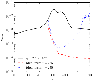
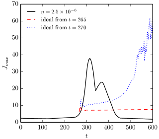
Figure 11: Time histories of $u_{max}$ and $J_{max}$ from two restart runs with $\eta$ set to zero. The black sold lines correspond to the original Run B3; red dashed lines and blue dotted lines represent restart runs from $t=265$ and $t=270$, respectively.

We now address the important question of what causes the onset in Case B. In previous discussion we suggest that resistive quasi-static evolution may actually bring the system (as in Case A) closer to an ideal stability threshold. Since Case B has a slightly higher initial magnetic energy than Case A, it is possible that resistive quasi-static evolution may eventually cause the system to pass through an ideal stability threshold. To further examine this possibility, we take the simulation B3 and restart at different times with $\eta$ set to zero. Figure 11 shows the time histories of $u_{max}$ and $J_{max}$ from two runs, restarted from $t=265$ and $t=270$, respectively. For the restart run from $t=265$, the plasma flow is quickly damped away by friction and viscosity, and the system relaxes to a new equilibrium and stays there. On the contrary, for the restart run from $t=270$, the plasma flow first decays and appears to be settling down initially but eventually starts to increase at $t\simeq 350$. That leads to the formation of intense current sheets, sufficiently intense that they eventually become under-resolved. These results suggest that the system is still within an ideal stability threshold at $t=265$, but has passed through the stability threshold at $t=270$. The current sheets formed after the onset of the instability bear similarity with the ones caused by ideal coalescence and kink instabilities (Longcope & Strauss, 1994b, a; Lionello et al., 1998a, b; Hood et al., 2009). However, due to the lack of ignorable coordinates in the equilibrium, analyzing the nature of the instability is a rather difficult task.

Although these results suggest that the onset may be caused by crossing an ideal MHD stability threshold, it is also possible that the system becomes resistively unstable before it reaches the ideal stability threshold. Formally we can analyze the resistive instability by assuming that the background is not evolving, and linearizing Equations (1) and (2), which yields the following eigenvalue problem:

$$i\omega\Omega=\mathbf{B}\cdot\nabla\tilde{J}+[\tilde{A},J],$$ (20)

$$i\omega\tilde{A}=\mathbf{B}\cdot\nabla\phi+\eta\nabla_{\perp}^{2}\tilde{A}.$$ (21)

Here $\tilde{A}$ and $\tilde{J}$ denote the linear perturbations of the flux function and current density, respectively; and we have again neglected viscosity and friction. It has been previously found that as the system just crosses the resistive stability threshold in line-tied systems, the linear growth rate scales linearly with $\eta$ (Delzanno & Finn, 2008; Huang & Zweibel, 2009). The reason is that near the stability threshold, the unstable mode is so slowly growing such that the inertia term $i\omega\Omega$ in Equation (20) is negligible. In this regime, the resistive instability is virtually indistinguishable from resistive quasi-static diffusion. However, as the system evolves further away from the stability threshold, the growth rate is expected to scale as $\sim\eta^{\alpha}$, with $0<\alpha<1$, and becomes distinguishable from resistive diffusion. To further examine this possibility requires a clear separation between the resistive diffusion time scale $\sim 1/\eta$ and the resistive instability time scale $\sim\eta^{-\alpha}$, which is beyond the parameter regimes we are able to probe and is left to a future study.

5.3 Measuring the “Distance” Between Field Line Mappings

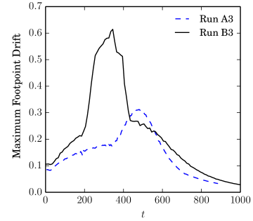
Figure 12: Time histories of maximum footpoint drift between two consecutive snapshots separated by one Alfvén transit time for Run A3 and Run B3.

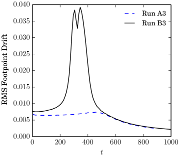
Figure 13: Time histories of root mean square footpoint drift between two consecutive snapshots separated by one Alfvén transit time for Run A3 and Run B3.

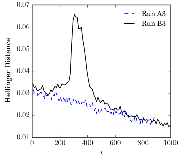
Figure 14: Time histories of the Hellinger difference between two consecutive snapshots of field line mapping separated by one Alfvén transit time for Run A3 and Run B3.

In Section 4 we present two cases where the evolutions of field line mapping follow qualitatively different behavior. In the first case governed by resistive quasi-static evolution, Run A3, the field line mapping appears to deform gradually; whereas in the second case, Run B3, the field line mapping rapidly changes to a qualitatively different pattern during the onset phase. Although the difference between the two cases is rather obvious to the human eye, how to translate this qualitative observation to a precise quantitative definition of magnetic reconnection in three dimensions remains an open question. To further address this issue, we ask the important question: “Given two consecutive snapshots of field line mappings, how do we measure how different they are?”

A simple measure is the maximum footpoint drift between two consecutive snapshots separated by one Alfvén transit time. However, as shown by the time histories of maximum footpoint drift in Figure 12, the two cases A3 and B3 appear to be qualitatively similar. In both cases, the maximum footpoint drift starts with a similar value $\simeq 0.1$, which gradually increases at later time, reaches a peak and then decays. The peak value of maximum footpoint drift in case B3 is approximately a factor of two higher than that in A3, which does not seem very significant. The problem of taking the maximum value of footpoint drift is that, it tends to overemphasize the difference, especially when the field line mapping is highly distorted with large gradient, as in the present cases. This can be appreciated by a simple one dimensional analogy. Consider a one dimensional function with a strong gradient, e.g. $f_{1}(x)=\tanh(x/h)$ with $h\ll 1$, and a slightly shifted function $f_{2}(x)=f_{1}(x-h)$. Even though for all practical purposes $f_{1}(x)$ and $f_{2}(x)$ are very similar, the maximum value of $\left|f_{1}(x)-f_{2}(x)\right|$ is of order unity. In this case, instead of using the maximum value, the $L^{2}$ norm of the difference

$$\left|\left|f_{1}(x)-f_{2}(x)\right|\right|_{2}\equiv\left(\int\left|f_{1}(x)-f_{2}(x)\right|^{2}dx\right)^{1/2},$$ (22)

is a better measure of the “distance” between the two functions.

Likewise, given two field line mappings $\mathbf{x}_{1}(\mathbf{x}_{b})$ and $\mathbf{x}_{2}(\mathbf{x}_{b})$, where $\mathbf{x}_{b}$ represents the coordinates at the bottom plate, we may measure the “distance” between them by the $L^{2}$ norm

$$\left|\left|\mathbf{x}_{1}(\mathbf{x}_{b})-\mathbf{x}_{2}(\mathbf{x}_{b})\right|\right|_{2}\equiv\left(\int\left|\mathbf{x}_{1}(\mathbf{x}_{b})-\mathbf{x}_{2}(\mathbf{x}_{b})\right|^{2}d^{2}x_{b}\right)^{1/2}.$$ (23)

In our diagnostics, we approximate the $L^{2}$ norm by the root mean square (RMS) footpoint drift of the sampled field lines, and Figure 13 shows the time histories of the RMS footpoint drift, for the two cases. As we can see, the $L^{2}$ norm gives a sharp distinction between the two cases during the onset phase of case B3.

Another possible way of measuring the distance between two mappings is through coarse graining the field line connectivity. First we divide the bottom plate and the top plate into $n\times n$ equal-sized cells for each of them. The coarse-grained representation of a field line mapping is the probability distribution $P=\{p_{ij}\}$, where $p_{ij}$ is the probability of a field line to connect the $i^{th}$ cell at the bottom and the $j^{th}$ cell at the top. Here again we make use of the doubly periodic boundary condition in defining field line connection between the two plates, such that bottom plate of the simulation box is exactly mapped to the top plate of the simulation box (see Figure 2). The probability distribution $\{p_{ij}\}$ satisfies the relation

$$\sum_{ij}p_{ij}=1.$$ (24)

After coarse-graining the field line mappings into probability distributions, we can measure the distance between two mappings by a proper measure of the distance between probability distributions. The motivation behind the coarse-graining approach is that, if the field line mapping deforms gradually in time, the probability distributions between two consecutive snapshots should be very similar, even though footpoints of individual field lines may drift a large distance.

Given two probability distributions $P=\{p_{ij}\}$ and $Q=\{q_{ij}\}$, there are numerous standard ways to quantify the difference between them [see, e.g. (DasGupta, 2008), Chapter 2, for an overview]. Here we employ the Hellinger distance $H(P,Q)$, defined as

$$H(P,Q)\equiv\frac{1}{\sqrt{2}}\sqrt{\sum_{ij}\left(\sqrt{p_{ij}}-\sqrt{q_{ij}}\right)^{2}}=\sqrt{1-\sum_{ij}\sqrt{p_{ij}q_{ij}}}.$$ (25)

The Hellinger distance satisfies the inequality $0\leq H(P,Q)\leq 1$. We divide each of the two end plates into $10\times 10$ cells, and calculate the Hellinger distance between two consecutive field line mappings separated by one Alfvén time by using the sampled field lines to estimate the probability distributions. Figure 14 shows the resulting time histories of Hellinger distance for the two cases A3 and B3. As can be seen from the two curves in Figure 14, the Hellinger distance is also very effective in distinguishing the onset phase and the quasi-static phase.

6 Summary and Conclusion

In this study, we find two distinct phases in our simulations on resistive relaxation of 3D force-free equilibria. In the phase governed by resistive quasi-static evolution, it is found that kinetic energy tends to be high, and field line mapping can change rapidly in regions where neighboring field lines strongly exponentiate from each other (i.e. high-$\sigma$ regions). During this phase, the evolution time scale $\sim 1/\eta$, as in resistive diffusion. Whether we would call the change of field line mapping “reconnection” is to some extent a matter of definition. As we have seen, even though the mapping of individual field lines can change rapidly, the overall pattern of the mapping appears to deform gradually rather than to undergo rapid qualitative change. Therefore, it may be more appropriate to call the rapid change of field line connectivity and high induced plasma flow in high-$\sigma$ regions during this phase “enhanced resistive diffusion” rather than “reconnection”. On the other hand, we also find that in some cases resistive quasi-static evolution can cause an ideally stable initial force-free equilibrium to pass through a stability threshold, leading to an “onset” phase. During this onset phase, intense current filaments develop, and the field line mapping change rapidly to a qualitatively different pattern on a timescale faster than $\sim 1/\eta$. The plasma flow exhibits signatures of inflow and outflow in the vicinities of current filaments. When the same initial condition is relaxed with different $\eta$, it is found that the current filaments become more intense the smaller the $\eta$ is. The presence of all these hallmarks of reconnection suggests that the change of field line connectivity in this onset phase may be more properly designated as “reconnection”. Because of the different scaling relations with respect to $\eta$, the difference between the two phases will become more distinct the smaller the $\eta$ is.

Our results illustrate a fundamental difference between 2D and 3D reconnection. In 2D the breaking of magnetic field line connectivity occurs in thin current sheets, therefore is much more closely coupled with magnetic energy conversion and dissipation; whereas in 3D the breaking of magnetic field line connectivity does not require a large current density and, therefore, is not directly associated with a large energy release. For this reason, a proper definition of reconnection becomes a tricky issue. If we consider magnetic energy conversion and dissipation as one of the hallmarks of magnetic reconnection, then we must conclude that rapid change of field line connectivity appears to be necessary, but insufficient as a signature of fast reconnection. Nonetheless, our results show that the meaning of the ideal constraints on magnetic field evolution is very subtle in 3D. Because of the exponential sensitivity, strict conservation of field line mapping as dictated by ideal MHD is essentially impossible in a generic, high-$\sigma$ 3D magnetic field. On the other hand, the fact the field line mapping can undergo gradual deformation even in the presence of a large apparent field line drift also calls for quantification of approximate conservation of ideal constraints other than direct measurement of individual footpoint drift. The measures of $L_{2}$ norm and Hellinger distance in Section 5.3 represent our preliminary attempt in this direction.

The process of current sheet formation during the onset phase requires further investigation. When the evolution deviates from the force-free condition $\mathbf{B}\cdot\nabla J=0$ due to some instability, the large gradient in $J$ implies the likelihood of developing a large $dJ/d\ell$, where $d\ell$ is the differential distance along a field line. A large $dJ/d\ell$ implies a large current across the magnetic field, for otherwise the current density would not be divergence free. The force associated with current across the field lines must be balanced by inertia. This is just what is implied by Equation (1): a large $dJ/d\ell$ implies a large time derivative in the vorticity of the flow $\Omega$. Although the reported simulations have sufficient dissipation to prevent Alfvén waves from bouncing back and forth, the relaxation of $dJ/d\ell$ back to zero occurs by Alfvén waves. As shown in (Boozer, 2014), Alfvén wave propagation in a high-$\sigma$ region turns the part of $J$ that is not constant along a field line into a current ribbon of exponentially high current density as well as producing a vortex ribbon [see also (Similon & Sudan, 1989)]. The current and vortex ribbon can be rapidly dissipated by resistivity or viscosity. Moreover, this mechanism can take place without the mediation of instabilities, as the large gradient in $J$ implies that any small perturbation in $\mathbf{B}$ can potentially leads to a large $dJ/dl$. Therefore, a general conclusion is that a high-$\sigma$ force-free equilibrium is very fragile and can hardly remain quiescent.

From a broader perspective, the interesting finding that resistive quasi-static evolution can lead to an onset of instability and subsequent formation of thin current sheets may have profound implications on Parker’s “topological dissipation” scenario of coronal heating (Parker, 1972). In this scenario, it is suggested that when the magnetic field lines in solar coronal loops become entangled due to footpoint motions on the photosphere, the ideal magnetostatic equilibrium of the entangled field develops current singularities (i.e. tangential discontinuities in magnetic field). In the presence of small but finite resistivity, the current singularities can dissipate resistively and heat the corona. Parker’s proposal has since become the famous Parker problem and has stimulated a substantial amount of debate that continues to this day (van Ballegooijen, 1985; Zweibel & Li, 1987; Ng & Bhattacharjee, 1998; Craig & Sneyd, 2005; Low, 2006; Janse & Low, 2009; Huang et al., 2009, 2010; Janse & Low, 2010; Aly & Amari, 2010; Janse et al., 2010; Low, 2010; Craig, 2010; Pontin & Huang, 2012; Low, 2013). The Parker problem is usually posed as an ideal MHD problem, where the key question is whether the minimum energy equilibrium for a given magnetic topology, assuming ideal MHD constraints are exactly conserved, contains tangential discontinuity or not. This formulation of the Parker problem is mathematically precise, and to some degree carries the connotation that formation of current sheets is purely an ideal MHD process, whereas the role of resistivity is to smooth out the singularity, to facilitate reconnection, and to dissipate the free energy. However, as neighboring field line exponentiation becomes significant as a natural consequence of continuous footpoint driving, conservation of ideal MHD constraints becomes subtle and may become overly restrictive. Furthermore, our results show that a small resistivity can cause an otherwise ideally stable equilibrium to break loose and subsequently develop much more intense current filaments. Therefore, it appears that resistivity can play an active, albeit subtle role in the formation of current sheets. Consequently, the physically relevant question may not be the ideal problem, but the resistive problem in the limit of very small $\eta$. This viewpoint has previously been emphasized by Bhattacharjee & Wang (1991) and now corroborated by the present study. A similar onset of instability has been reported in recent studies on resistive relaxation of braided force-free coronal loops (Wilmot-Smith et al., 2010; Pontin et al., 2011). However, the onset time is approximately independent of $\eta$ in the reported simulations, whereas the onset time $\sim 1/\eta$ in the present study. Therefore, the instabilities in the two types of studies are likely to be qualitatively different.

The enhanced resistive diffusion reported in this work is conceptually different from the mechanism of breaking ideal MHD frozen-in condition via turbulent Richardson advection as proposed by Eyink et al. (2013). In their scenario, the spontaneously stochastic trajectories caused by turbulent flow bring together field lines from distances far apart, which, as Eyink et al. argued, results in breakdown of the frozen-in condition even in the limit $\eta\to 0$. On the other hand, the enhanced resistive diffusion in the present work is caused by the stochasticity in magnetic field line mapping. The plasma flow does not become turbulent in either the quiescent or onset phases. Therefore, Alfvén’s frozen-in theorem is expected to be satisfied as $\eta\to 0$.

Finally, we remark on some limitations of the present study. The initial conditions employed in this study are constructed by integrating $\mathbf{B}\cdot\nabla J=0$ from a given flux function $A_{0}$ at the mid-plane of the simulation box; these initial conditions may not be representative of the generic force-free equilibria that arise more naturally, e.g. by imposing footpoint motion at the boundaries as in Parker’s model. The exponent $\sigma$ in this work is rather modest due to the limitation of numerical resolution, while high-$\sigma$ regions concentrate in layers. In astrophysical or space plasmas, the exponent $\sigma$ is expected to be significantly higher, and high-$\sigma$ regions could be more volume-filling. Other physical effects known to be important to reconnection, e.g. Hall effect, electron pressure and inertia, are also not included. The conclusions of this study should be further examined under those conditions.

Appendix A Construction of Force-Free Equilibrium

The initial force-free equilibrium for simulation is constructed by integrating

$$\mathbf{B}\cdot\nabla J=\partial_{z}J+\left[A,J\right]=0$$ (A1)

along the $z$ direction from a prescribed $A=A_{0}(\mathbf{x}_{\perp})$ at $z=0$. Although Equation (A1) can in principle be integrated with any standard numerical scheme, because the constructed equilibrium is usually very delicate due to high field line exponentiation, it is important to employ exactly the same discretization scheme for both the simulation code and the integration; otherwise, the discrepancy in discretization errors due to different numerical schemes may result in non-negligible unbalanced force when the constructed equilibrium is used as an initial condition for simulation.

The simulation code employs staggered grids for variables $\phi$ and $A$ along the $z$ direction. That means that $\mathbf{B}\cdot\nabla J$ is evaluated at the middle point between two adjacent grid points where $A$ resides. Specifically, the discretized representation for $\mathbf{B}\cdot\nabla J$ between the $i$^th and $(i+1)$^th grid points is

$$\left(\mathbf{B}\cdot\nabla J\right)_{i+1/2}=\frac{J_{i+1}-J_{i}}{\Delta z}+\left[\frac{A_{i+1}+A_{i}}{2},\frac{J_{i+1}+J_{i}}{2}\right],$$ (A2)

where $\Delta z$ is the grid size along $z$; the Poisson bracket is calculated by a standard pseudospectral method, i.e. derivatives are carried out in the Fourier space and products are calculated in the real space. When the discretized representation (A2) is used in Equation (A1), it becomes an implicit scheme that $A_{i+1}$ can be determined by inverting a nonlinear equation if $A_{i}$ is known. This nonlinear inversion is solved iteratively until a convergence criterion is satisfied. In this work, the convergence criterion is set to be $\int\left(\mathbf{B}\cdot\nabla J\right)_{i+1/2}^{2}d^{2}x<10^{-25}.$

The corresponding problem in full MHD instead of RMHD is constructing a force-free equilibrium from all three components of $\mathbf{B}$ given on a plane. This is an important problem in solar physics due to the great interest in extrapolating the coronal magnetic field from the photospheric magnetograms [see, e.g. (Wiegelmann & Sakurai, 2012) for a recent review and references therein]. A straightforward generalization of the procedure here to full MHD is the well-known upward integration method (Nakagawa, 1974; Wu et al., 1990), which integrates $\nabla\times\mathbf{B}=\alpha\mathbf{B}$ and $\nabla\cdot\mathbf{B}=0$ simultaneously from the vector $\mathbf{B}$ given at a plane (assumed to be the $z=0$ plane in the following discussion). First the variable $\alpha$ is determined by $z$ component of $\nabla\times\mathbf{B}=\alpha\mathbf{B}$:

$$\partial_{x}B_{y}-\partial_{y}B_{x}=\alpha B_{z}.$$ (A3)

The remaining two components of $\nabla\times\mathbf{B}=\alpha\mathbf{B}$ then give the $z$ derivatives of $B_{x}$ and $B_{y}$:

$$\partial_{z}B_{x}=\alpha B_{y}+\partial_{x}B_{z},$$ (A4)

$$\partial_{z}B_{y}=-\alpha B_{x}-\partial_{y}B_{z}.$$ (A5)

Finally, the $z$ derivative of $B_{z}$ is obtained from the condition $\nabla\cdot\mathbf{B}=0$:

$$\partial_{z}B_{z}=-\partial_{x}B_{x}-\partial_{y}B_{y}.$$ (A6)

Equations (A3) – (A6) can be employed to integrate all three components of $\mathbf{B}$ to the next constant-$z$ plane and the whole procedure is then repeated.

However, the upward integration method in full MHD is known to be mathematically ill-posed and numerically unstable [see, e.g. the discussions in (Low & Lou, 1990; Amari et al., 1997; Démoulin et al., 1997)]. In particular, difficulties may arise near photospheric polarity inversion lines where $B_{z}=0$ (which are present in most solar applications), as Equation (A3) requires that the left hand side $\partial_{x}B_{y}-\partial_{y}B_{x}$ must vanish as well. Therefore, the three components of $\mathbf{B}$ at $z=0$ cannot be arbitrarily prescribed but must satisfy the above mentioned constraint. Although $\alpha$ can in principle be obtained by applying l’Hôspital’s rule if the constraint is satisfied (Cuperman et al., 1991), any arbitrary small errors in $\mathbf{B}$ can violate the constraint and render the boundary condition incompatible with the force-free condition. Another drawback of the upward integration method for coronal magnetic field extrapolation is that the desirable asymptotic condition that the magnetic field vanishes at infinity cannot be guaranteed because boundary conditions are only imposed at $z=0$. Direct integration of Equations (A3) – (A6) usually leads to exponential growth of the magnetic field away from the boundary, and the solution is very sensitive to tiny changes of the boundary conditions. Various techniques have been proposed to regularize the method (Cuperman et al., 1990; Démoulin et al., 1992), but cannot be considered as fully successful.

In the context of the present study, however, the above mentioned limitations of the upward integration method are largely alleviated. The assumption of a strong $B_{z}$ ensures that Equation (A3) is well-conditioned. Furthermore, the force-free equations are only integrated over a finite distance, therefore the asymptotic behavior of $\mathbf{B}$ is not a concern. It remains an interesting open question whether a force-free equilibrium can be constructed for full MHD by a method similar to the one presented here under these conditions.

References

- Aly & Amari (2010) Aly, J. J., & Amari, T. 2010, Astrophys. J. Lett., 709, L99
- Amari et al. (1997) Amari, T., Aly, J. J., Luciani, J. F., Boulmezaoud, T. Z., & Mikic, Z. 1997, Solar Physics, 174, 129
- Bhattacharjee & Wang (1991) Bhattacharjee, A., & Wang, X. 1991, Astrophys. J., 372, 321
- Biskamp (2000) Biskamp, D. 2000, Magnetic Reconnection in Plasmas (Cambridge University Press)
- Boozer (2012a) Boozer, A. H. 2012a, Phys. Plasmas, 19, 092902
- Boozer (2012b) —. 2012b, Phys. Plasmas, 19, 112901
- Boozer (2013) —. 2013, Phys. Plasmas, 20, 032903
- Boozer (2014) —. 2014, Phys. Plasmas, in press
- Craig (2010) Craig, I. J. D. 2010, Solar Physics, 266, 293
- Craig & Sneyd (2005) Craig, I. J. D., & Sneyd, A. D. 2005, Solar Physics, 232, 41
- Cuperman et al. (1991) Cuperman, S., Démoulin, P., & Semel, M. 1991, Astron. Astrophys., 245, 285
- Cuperman et al. (1990) Cuperman, S., Ofman, L., & Semel, M. 1990, Astron. Astrophys., 230, 193
- DasGupta (2008) DasGupta, A. 2008, Asymptotic Theory of Statistics and Probability (New York: Springer Science+Business Media, LLC)
- Delzanno & Finn (2008) Delzanno, G. L., & Finn, J. M. 2008, Phys. Plasmas, 15, 032904
- Démoulin et al. (1992) Démoulin, P., Cuperman, S., & Semel, M. 1992, Astron. Astrophys., 263, 351
- Démoulin et al. (1997) Démoulin, P., Hénoux, J. C., Mandrini, C. H., & Priest, E. R. 1997, Solar Physics, 174, 73
- Démoulin et al. (1996) Démoulin, P., Hénoux, J. C., Priest, E. R., & Mandrini, C. H. 1996, Astron. Astrophys., 308, 643
- Dmitruk & Gómez (1999) Dmitruk, P., & Gómez, D. O. 1999, Astrophys. J., 527, L63
- Dmitruk et al. (2003) Dmitruk, P., Gómez, D. O., & Matthaeus, W. H. 2003, Phys. Plasmas, 10, 3584
- Eyink et al. (2013) Eyink, G., Vishniac, E., Lalescu, C., et al. 2013, Nature, 497, 466
- Finn et al. (2014) Finn, J. M., Billey, Z., Daughton, W., & Zweibel, E. 2014, Plasma Phys. Control. Fusion, 56, 064013
- Gekelman et al. (2014) Gekelman, W., Van Compernolle, B., DeHass, T., & Vincena, S. 2014, Plasma Phys. Control. Fusion, 56, 064002
- Greene (1993) Greene, J. M. 1993, Phys. Fluids B, 5, 2355
- Hesse et al. (2005) Hesse, M., Forbes, T. G., & Birn, J. 2005, Astrophys. J., 631, 1227
- Hesse & Schindler (1988) Hesse, M., & Schindler, K. 1988, J. Geophy. Res., 93, 5559
- Hood et al. (2009) Hood, A. W., Browning, P. K., & Van der Linden, R. A. M. 2009, Astron. Astrophys., 506, 913
- Huang et al. (2009) Huang, Y.-M., Bhattacharjee, A., & Zweibel, E. G. 2009, Astrophys. J. Lett., 699, L144
- Huang et al. (2010) —. 2010, Phys. Plasmas, 17, 055707
- Huang & Zweibel (2009) Huang, Y.-M., & Zweibel, E. G. 2009, Phys. Plasmas, 16, 042102
- Janse & Low (2009) Janse, A. M., & Low, B. C. 2009, Astrophys. J., 690, 1089
- Janse & Low (2010) —. 2010, Astrophys. J., 722, 1844
- Janse et al. (2010) Janse, A. M., Low, B. C., & Parker, E. N. 2010, Phys. Plasmas, 17, 092901
- Kadomtsev & Pogutse (1974) Kadomtsev, B. B., & Pogutse, O. P. 1974, Sov. Phys. JETP, 38, 283
- Lawrence & Gekelman (2009) Lawrence, E. E., & Gekelman, W. 2009, PRL, 103, 105002
- Lionello et al. (1998a) Lionello, R., Schnack, D. D., Einaudi, G., & Velli, M. 1998a, Phys. Plasmas, 54, 3722
- Lionello et al. (1998b) Lionello, R., Velli, M., Einaudi, G., & Mikić, Z. 1998b, Astrophys. J., 494, 840
- Longcope & Strauss (1994a) Longcope, D. W., & Strauss, H. R. 1994a, Astrophys. J., 437, 851
- Longcope & Strauss (1994b) —. 1994b, Astrophys. J., 426, 742
- Longcope & Sudan (1994) Longcope, D. W., & Sudan, R. N. 1994, Astrophys. J., 437, 491
- Low (2006) Low, B. C. 2006, Astrophys. J., 649, 1064
- Low (2010) —. 2010, Solar Physics, 266, 277
- Low (2013) —. 2013, Astrophys. J., 768, 7
- Low & Lou (1990) Low, B. C., & Lou, Y. Q. 1990, Astrophys. J., 352, 343
- Nakagawa (1974) Nakagawa, Y. 1974, Astrophys. J., 190, 437
- Ng & Bhattacharjee (1998) Ng, C. S., & Bhattacharjee, A. 1998, Phys. Plasmas, 5, 4028
- Ng & Bhattacharjee (2008) —. 2008, Astrophys. J., 675, 899
- Ng et al. (2012) Ng, C. S., Lin, L., & Bhattacharjee, A. 2012, Astrophys. J., 747, 109
- Parker (1972) Parker, E. N. 1972, Astrophys. J., 174, 499
- Pontin (2011) Pontin, D. I. 2011, Adv. Space Res., 47, 1508
- Pontin & Huang (2012) Pontin, D. I., & Huang, Y.-M. 2012, Astrophys. J., 756, 7
- Pontin et al. (2011) Pontin, D. I., Wilmot-Smith, A. L., Hornig, G., & Galsgaard, K. 2011, Astron. Astrophys., 525, A57
- Priest & Démoulin (1995) Priest, E. R., & Démoulin, P. 1995, J. Geophy. Res., 100, 23443
- Priest & Forbes (2000) Priest, E. R., & Forbes, T. 2000, Magnetic reconnection : MHD theory and applications (Cambridge University Press)
- Priest et al. (2003) Priest, E. R., Hornig, G., & Pontin, D. I. 2003, Journal of Geophysical Research, 108, 1285
- Rappazzo & Parker (2013) Rappazzo, A. F., & Parker, E. N. 2013, Astrophys. J. Lett., 773, L2
- Rappazzo et al. (2007) Rappazzo, A. F., Velli, M., Einaudi, G., & Dahlburg, R. B. 2007, Astrophys. J., 657, L47
- Rappazzo et al. (2008) —. 2008, Astrophys. J., 677, 1348
- Richardson & Finn (2012) Richardson, A. S., & Finn, J. M. 2012, Commun. Nonlinear Sci. Numer. Simulat., 17, 2132
- Schindler et al. (1988) Schindler, K., Hesse, M., & Birn, J. 1988, J. Geophy. Res., 93, 5547
- Schnack et al. (1986) Schnack, D. D., Barnes, D. C., Mikić, Z., et al. 1986, Computer Physics Communications, 43, 17
- Similon & Sudan (1989) Similon, P. L., & Sudan, R. N. 1989, Astrophys. J., 336, 442
- Strauss (1976) Strauss, H. R. 1976, Phys. Fluids, 19, 134
- Strauss & Otani (1988) Strauss, H. R., & Otani, N. F. 1988, Astrophys. J., 326, 418
- Titov (2007) Titov, V. S. 2007, Astrophys. J., 660, 863
- Trefethen & Bau (1997) Trefethen, L. N., & Bau, III, D. 1997, Numerical Linear Algebra (SIAM Philadelphia)
- van Ballegooijen (1985) van Ballegooijen, A. A. 1985, Astrophys. J., 298, 421
- Wiegelmann & Sakurai (2012) Wiegelmann, T., & Sakurai, T. 2012, Living Reviews in Solar Physics, 9, doi:10.12942/lrsp-2012-5
- Wilmot-Smith et al. (2010) Wilmot-Smith, A. L., Pontin, D. I., & Hornig, G. 2010, Astron. Astrophys., 516, A5
- Wu et al. (1990) Wu, S. T., Sun, M. T., Chang, H. M., Hagyard, M. J., & Gary, G. A. 1990, Astrophys. J., 362, 698
- Yamada et al. (2010) Yamada, M., Kulsrud, R., & Ji, H. 2010, Rev. Mod. Phys., 82, 603
- Zweibel & Li (1987) Zweibel, E. G., & Li, H.-S. 1987, Astrophys. J., 312, 423
- Zweibel & Yamada (2009) Zweibel, E. G., & Yamada, M. 2009, Annu. Rev. Astron. Astrophys., 47, 291