Brillouin zone unfolding of Complex Bands in a nearest neighbour Tight Binding scheme

Abstract

Complex bands $\bm{k}^{\perp}(E)$ in a semiconductor crystal, along a general direction $\bm{n}$, can be computed by casting Schrödinger’s equation as a generalized polynomial eigenvalue problem. When working with primitive lattice vectors, the order of this eigenvalue problem can grow large for arbitrary $\bm{n}$. It is however possible to always choose a set of non-primitive lattice vectors such that the eigenvalue problem is restricted to be quadratic. The complex bands so obtained need to be unfolded onto the primitive Brillouin zone. In this paper, we present a unified method to unfold real and complex bands. Our method ensures that the measure associated with the projections of the non-primary wavefunction onto all candidate primary wavefunctions is invariant with respect to the energy $E$.

Keywords: Brillouin Zone unfolding, Complex bands, Tight Binding.

1 Introduction

Complex bandstructure $\bm{k}(E)$ describes the properties of both propagating and evanescent electronic states in semiconductor crystals. Evanescent states have imaginary or complex wavevectors and govern tunneling phenomena [1] in semiconductor devices. The relative importance of these phenomena has increased with every reduction in the dimensions of these devices. Complex bandstructure is also used to predict barrier heights of metal-semiconductor interfaces [2] and band lineups at semiconductor heterointerfaces [3], via the theory of Virtual Induced Gap States (ViGS). An accurate computation of complex bandstructure is hence essential for the continued scaling and materials engineering of electronic devices, with an aim of improving performance.

Of the many approaches to bandstructure calculation, the $sp^{3}d^{5}s^{*}$ nearest neighbour empirical tight binding method [4, 5] has proven to represent a good trade-off between accuracy and computational efficiency. Complex bands along a given transport direction $\bm{n}$ can be computed within this framework by casting Schrödinger’s equation as a Generalized Polynomial Eigenvalue Problem (GPEP), as described in [6] for the $[001]$ direction. This method can be extended [7] to a general $\bm{n}$, by working with a set of primitive lattice vectors $\bm{u}_{1},\bm{u}_{2},\bm{u}_{3}$ that are adapted to the plane perpendicular to $\bm{n}$, i.e. $\bm{u}_{1}\cdot\bm{n}>0$ and $\bm{u}_{2},\bm{u}_{3}\perp\bm{n}$. As shown in Figure 1 and described in Section 2, the order of the GPEP depends on $\bm{n}$, since $\bm{u}_{1}$ is not necessarily parallel to $\bm{n}$.

Hence, the computation of complex bands along an arbitrary $\bm{n}$ could involve a GPEP of large order. Moreover, arbitrary extrinsic strain can lead to a GPEP of large order even for transport along simple directions like $[111]$. Robust solution of a GPEP of large order is a challenging [8] problem, sometimes introducing large errors. The order of the GPEP can be limited to be quadratic, even for arbitrary $\bm{n}$, by working with a non-primitive set of lattice vectors [9] $\bm{f}_{1},\bm{f}_{2},\bm{f}_{3}$ such that $\bm{f}_{1}\parallel\bm{n}$ and $\bm{f}_{2},\bm{f}_{3}\perp\bm{n}$. Energy bands obtained using this non-primitive cell correspond, however, to primitive cell energy bands that have been folded onto the smaller, non-primitive Brillouin zone. These bands have to be unfolded onto the primitive Brillouin zone.

Zone folding and unfolding have been studied extensively for the case of real bands [10, 11, 12, 13, 14, 15]. Computation of real and complex bands differ in their choice of basis, Bloch sums [16] (which represent the full periodicity of the lattice) for the former, whereas Layer Bloch sums [6] (which only represent periodicity in directions perpendicular to $\bm{n}$) for the latter. Further, unlike wavefunctions with real wavevectors, those with complex wavevectors need to be normalized carefully. The imaginary part of the wavevector enters into the normalization constant. Ignoring this yields different measures for the norm of the wavefunction for different $Im(\bm{k})$. It is hence not obvious whether the zone unfolding method derived for real bands can be used to unfold complex bands along a general $\bm{n}$. Note that [9] applies the scheme available for real bands to the case of complex bands without providing any rigorous justification.

In this paper, we show rigorously that the method of unfolding can indeed be used for complex bands too, provided some modifications are included. Our modifications ensures that the measure associated with the projections of the non-primary wavefunction onto all candidate primary wavefunctions is invariant with respect to the energy $E$, for real and complex bands. This invariance is especially important when the supercell technique [12] is used to compute the bandstructure of disordered materials.

This paper is structured as follows. In Section 2, we setup notation and describe the method of computing complex bands along a general $\bm{n}$ using plane adapted primitive lattice vectors. Section 3 deals with using non-primitive vectors, and presents the modified zone unfolding method. Finally, Section 4 applies our method by to the case of complex bands along the $[110]$ direction in Silicon and summarizes the paper.

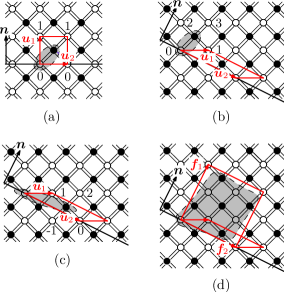
Figure 1: Two dimensional crystal showing primitive and non-primitive lattice vectors adapted to the line perpendicular to transport direction $\bm{n}$. The crystal has a square lattice and a motif consisting of one $\circ$ (at $\bm{\nu}=0$) and one $\bullet$. In each case, the motif is outlined by a dashed line and shaded gray. (a) Primitive cell when $\bm{u}_{1}\parallel\bm{n}$. (b) Primitive cell when $\bm{u}_{1}\nparallel\bm{n}$, using the same motif as in (a). (c) Primitive cell for the same $\bm{n}$ as in (b), but with a motif such that $\bullet$ is within the cell. (d) Non-primitive cell ($\mathcal{N}_{c}=5$) for the same $\bm{n}$ as in (b). In cases (a), (b), (c), the numbers indicate the $s_{1}$ values (see (1) ) of the nearest neighbours of the $\bullet$ of the motif. The corresponding GPEP (5) is of order $\mathcal{O}=2\times\max(|s_{1}|)$.

2 Complex bands using a primitive unit cell

The primitive vectors $\bm{u}_{1}$, $\bm{u}_{2}$, $\bm{u}_{3}$ are constructed using the method described in [17]. A point in the lattice is represented as

$$\bm{\rho}(s_{1},s_{2},s_{3}) =s_{1}\bm{u}_{1}+\underbrace{s_{2}\bm{u}_{2}+s_{3}\bm{u}_{3}}_{\bm{\rho}^{\parallel}(s_{2},s_{3})}$$ (1)

where $s_{1},s_{2},s_{3}$ are integers. Correspondingly, a vector in reciprocal space is $\bm{k}=\bm{k}^{\parallel}+\bm{k}^{\perp}$, such that $\bm{k}^{\perp}$ is along $\bm{n}$. The crystal is constructed by associating a motif of atoms with each lattice point. For crystals having a Zinc Blende structure, the motif has two atoms. Let $\bm{\nu}_{m}$, $m=1,2$ represent the positions of these atoms with respect to the lattice point. We set $\bm{\nu}_{1}=\bm{0}$ without any loss of generality.

There are $\mathcal{N}_{TB}=20$ orthonormal orbitals (10 Löwdin orbitals [18] of each spin type) associated with each atomic site in the $sp^{3}d^{5}s^{*}$ scheme. An orbital of type $\mu$, spin $\varsigma$ on an atom $m$ located at site $\bm{\rho}_{j}$ is given by $\langle{\bm{r}}|{\mu,\varsigma;\bm{\rho}_{j}+\bm{\nu}_{m}}\rangle=\phi_{\mu\varsigma}\big{(}\bm{r}-(\bm{\rho}_{j}+\bm{\nu}_{m})\big{)}$. Complex bands are obtained by expressing the wavefunction $\psi(\bm{r},\bm{k})=\langle{\bm{r}}|{\psi(\bm{k}^{\perp},\bm{k}^{\parallel})}\rangle$ as a linear combination of layer Bloch sums [6]. A layer Bloch sum is a linear superposition of orbitals on all similar atoms associated with a single lattice layer. Denoting the layer Bloch sum corresponding to orbital $\mu$ with spin $\varsigma$ on atom $m$ in layer $s_{1}=s$ as $\xi_{\mu\varsigma m}(\bm{r};s,\bm{k}^{\parallel})=\langle{\bm{r}}|{\mu,\varsigma;m,s,\bm{k}^{\parallel}}\rangle$, we have

$$\xi_{\mu\varsigma m}(\bm{r};s,\bm{k}^{\parallel})=\frac{1}{\sqrt{M_{\parallel}}}\sum_{j}^{(M_{\parallel})}e^{\iota\bm{k}^{\parallel}\cdot(\bm{\rho}^{\parallel}_{j}+s\bm{u}_{1}+\bm{\nu}_{m})}{\phi_{\mu\varsigma}(\bm{r}-(\bm{\rho}^{\parallel}_{j}+s\bm{u}_{1}+\bm{\nu}_{m}))}$$ (2)

where the symbol $\sum_{j}^{(M_{\parallel})}$ denotes a summation over $M_{\parallel}$ lattice sites (indexed by $j$), within a parallelogram with sides along $\bm{u}_{2},\bm{u}_{3}$. Periodic boundary conditions are imposed w.r.t this parallelogram. We thus write

$$|{\psi(\bm{k}^{\perp},\bm{k}^{\parallel})}\rangle=\sum_{\mu\varsigma m}\sum_{s}^{(M_{1})}c^{\mu\varsigma m}_{s}(\bm{k}^{\perp})|{\mu,\varsigma;m,s,\bm{k}^{\parallel}}\rangle$$ (3)

as a summation over $M_{1}$ lattice layers. Both $M_{\parallel}$ and $M_{1}$ are allowed to tend to infinity.

The periodicity of the lattice enforces a condition,

$$c_{s}^{\mu\varsigma m}(\bm{k}^{\perp})=e^{\iota\bm{k}^{\perp}\cdot\bm{u}_{1}}c_{s-1}^{\mu\varsigma m}(\bm{k}^{\perp}).$$ (4)

Using these layer Bloch sums as a basis, Schrödinger’s equation $\mathcal{H}|{\psi}\rangle=E|{\psi}\rangle$ can be written as a matrix equation $\forall s$,

$$\sum_{p}[{H}_{s,s-p}][{c}_{s-p}]+\left([{H}_{s,s}]-[1]E\right)[{c}_{s}]+\sum_{p}[{H}_{s,s+p}][{c}_{s+p}]=0$$ (5)

where $[c_{s}]$ is a column matrix of size $2\mathcal{N}_{TB}\times 1$ such that $[c_{s}]_{\mu\varsigma m}=c^{\mu\varsigma m}_{s}$ and $[H_{s^{\prime},s^{\prime\prime}}]$ is a matrix of size $2\mathcal{N}_{TB}\times 2\mathcal{N}_{TB}$ such that

$$[H_{s^{\prime},s^{\prime\prime}}]_{\mu^{\prime}\varsigma^{\prime}m^{\prime},\mu^{\prime\prime}\varsigma^{\prime\prime}m^{\prime\prime}}=\langle{\mu^{\prime},\varsigma^{\prime};m^{\prime},s^{\prime},\bm{k}^{\parallel}}|\mathcal{H}|{\mu^{\prime\prime},\varsigma^{\prime\prime};m^{\prime\prime},s^{\prime\prime},\bm{k}^{\parallel}}\rangle.$$ (6)

The summation in (5) is over all unique $p\neq 0$ such that the atom at $\bm{\rho}^{\parallel}+(s+p)\bm{u}_{1}+\bm{\nu}_{0}$ is a nearest neighbour of the atom at $s\bm{u}_{1}+\bm{\nu}_{1}$, for some $\bm{\rho}^{\parallel}$. Equation (5) is a generalized polynomial eigenvalue problem (of order $\mathcal{O}=2\times\max|p|$) with eigenvalue $\lambda=e^{\iota\bm{k}^{\perp}\cdot\bm{u}_{1}}$ and eigenvector $[c_{s}]$. Following [8], (5) is said to be $*$-palindromic, since $[H_{s,s}]$ is Hermitian and $[H_{s,s-p}]^{\dagger}=[H_{s-p,s}]=[H_{s,s+p}]$; the $\dagger$ refers to conjugate transpose. The eigenvalues $\lambda$ thus occur in reciprocal conjugate pairs, i.e. if $\lambda$ is an eigenvalue, then $\frac{1}{\lambda^{*}}$ is also an eigenvalue. Hence, the component of $\bm{k}^{\perp}(E)$ along the transport direction, $k^{\perp}(E)$, appears in conjugate pairs $(k^{\perp},k^{\perp*})$. Equation (5) can be solved for $k^{\perp}(E)$ by recasting it as a generalized linear eigenvalue problem involving matrices of size $2\cdot\mathcal{O}\cdot\mathcal{N}_{TB}\times 2\cdot\mathcal{O}\cdot\mathcal{N}_{TB}$.

The number of terms and the order $\mathcal{O}$ of (5) depend on $\bm{n}$. To see this, consider the toy two-dimensional crystal as shown in Figure 1. This crystal has a square lattice and a motif consisting of one $\circ$ and one $\bullet$. Each $\circ$ is bonded to four $\bullet$’s and vice versa. The numbers in Figure 1(a), (b), (c) give the values of $p$ required in (5) assuming $s=0$.

3 Complex bands using a Non-Primitive unit cell and a Modified Zone unfolding algorithm

Consider the non-primitive unit cell in Figure 1(d). Since $\bm{f}_{1}\parallel\bm{n}$, atoms within the motif bond to atoms belonging only to the same or neighbouring lattice layers. Thus, in the general case, we can ensure that the generalized polynomial eigenvalue problem is restricted to be quadratic, by working with non-primitive vectors $\bm{f}_{1}\parallel\bm{n},\bm{f}_{2}=\bm{u}_{2},\bm{f}_{3}=\bm{u}_{3}$. The volume of the non-primitive unit cell is an integral multiple $\mathcal{N}_{c}$ of that of the primitive cell, causing the the non-primitive Brillouin zone to be $1/\mathcal{N}_{c}$ as large as the primitive one. As an example, $\mathcal{N}_{c}=5$ in Figure 1(d). We choose the non-primitive unit cell to have the same origin as the primitive cell. We use upper case Roman and Greek letters to denote quantities related to the non-primitive scheme.

A non-primitive lattice point is given by

$$\bm{R}(t_{1},t_{2},t_{3}) =t_{1}\bm{f}_{1}+\underbrace{t_{2}\bm{f}_{2}+t_{3}\bm{f}_{3}}_{\bm{R}^{\parallel}(t_{2},t_{3})}$$ (7)

where $t_{1},t_{2},t_{3}$ are integers. A vector in reciprocal space is now $\bm{K}=\bm{K}^{\parallel}+\bm{K}^{\perp}$. The motif associated with each lattice point will have $2\mathcal{N}_{c}$ atoms, positioned at $\bm{\gamma}_{n}$, $n=1,2,\ldots,2\mathcal{N}_{c}$ w.r.t the lattice point. Since the primitive and non-primitive cells share a common origin, we set $\bm{\nu}_{1}=\bm{\gamma}_{1}=\bm{0}$. We denote the non-primitive layer Bloch sum (over $N_{\parallel}$ lattice sites) as $\Xi_{\mu\varsigma n}(\bm{r};t,\bm{K}^{\parallel})=\langle{\bm{r}}|{\mu,\varsigma;n,t,\bm{K}^{\parallel}}\rangle$ and wavefunction as $\Psi(\bm{r},\bm{K})=\langle{\bm{r}}|{\Psi(\bm{K}^{\perp},\bm{K}^{\parallel})}\rangle$. Writing

$$|{\Psi(\bm{K}^{\perp},\bm{K}^{\parallel})}\rangle=\sum_{\mu\varsigma n}\sum_{t}^{(N_{1})}C^{\mu\varsigma n}_{t}(\bm{K}^{\perp})|{\mu,\varsigma;n,t,\bm{K}^{\parallel}}\rangle,$$ (8)

we obtain $K^{\perp}(E)$ by solving the resulting generalized quadratic eigenvalue problem. Finally, $k^{\perp}(E)$ is computed from $K^{\perp}(E)$ using the modified zone unfolding algorithm described below.

It is important to recognize that working with large non-primitive cells could present numerical difficulties in the solution of the generalized quadratic eigenvalue problem. Poor quality eigenvalues and eigenvectors could render the zone unfolding method useless. This problem is expected to be most severe for eigenvalues corresponding to large $|Im(K^{\perp})|$, owing to the exponential nature of the factor $\lambda=e^{\iota\bm{K}^{\perp}\cdot\bm{f}_{1}}$. However, the problem is mitigated by the fact that our primary application, modelling of tunneling phenomena, only requires evanescent states having the smallest $|Im(K^{\perp})|$. Nevertheless, the most important reason for erroneous eigenvalues and eigenvectors is the use of the standard companion linearization scheme [8], which neglects the palindromic structure of the GPEP (as shown, for example, in [19] for the case of vibration analysis of fast trains, involving an eigenvalue problem with similar symmetry). The eigenvalues $\lambda$ hence no longer appear as $\lambda,\frac{1}{\lambda^{*}}$ pairs. The use of a structure preserving linearization [8, 20, 21] rectifies this issue, and has been shown to greatly improve the quality of the eigenvalues and eigenvectors. Thus, a careful choice of linearization and eigensolver is critical to the scalability of the method discussed in this paper to large non-primitive cells.

The essential idea in zone unfolding is to express a wavefunction obtained using a non-primitive cell as a linear combination of primitive cell wavefunctions. The process of unfolding then boils down to estimating the contributions of each of these primitive cell wavefunctions to the non-primitive cell wavefunction. In order to achieve this, both the non-primitive and primitive wavefunctions are written in terms of their constituent atomic orbitals.

3.1 Wavefunctions in terms of atomic orbitals

To remain consistent with the zone unfolding algorithm for real bands available in [12, 13], we use a slightly modified version of the layer Bloch sums to describe the zone unfolding procedure. Working with the non-primitive cell, we define a primed layer Bloch sum $\Xi^{\prime}_{\mu\varsigma n}(\bm{r};t,\bm{K}^{\parallel})=\langle{\bm{r}}|{\mu,\varsigma;n,t,\bm{K}^{\parallel}}\rangle^{\prime}$,

$$\Xi^{\prime}_{\mu\varsigma n}(\bm{r};t,\bm{K}^{\parallel})=\frac{1}{\sqrt{N_{\parallel}}}\sum_{j}^{(N_{\parallel})}e^{\iota\bm{K}^{\parallel}\cdot(\bm{R}^{\parallel}_{j}+t\bm{f}_{1})}\langle{\bm{r}}|{\mu,\varsigma;\bm{R}^{\parallel}_{j}+t\bm{f}_{1}+\bm{\gamma}_{n}}\rangle$$ (9)

Notice that this differs from the non-primary version of the layer Bloch sum defined in (2) only in the absence of the term $e^{\iota\bm{K}^{\parallel}\cdot\bm{\gamma}_{n}}$ preceding the atomic orbital. Following (8), we write

$$|{\Psi(\bm{K}^{\perp},\bm{K}^{\parallel})}\rangle=\sum_{\mu\varsigma n}\sum_{t}^{(N_{1})}C^{\prime\;\mu\varsigma n}_{t}(\bm{K}^{\perp})|{\mu,\varsigma;n,t,\bm{K}^{\parallel}}\rangle^{\prime},$$ (10)

where, we have similar to (4),

$$C_{t+1}^{\prime\;\mu\varsigma n}(\bm{K}^{\perp})=e^{\iota\bm{K}^{\perp}\cdot\bm{f}_{1}}C_{t}^{\prime\;\mu\varsigma n}(\bm{K}^{\perp})$$ (11)

Comparing the two expansions for the wavefunction (8), (10) we can relate the expansion coefficients in the primed basis to those obtained in the unprimed basis as

$$C^{\prime\;\mu\varsigma n}_{t}(\bm{K}^{\perp})=e^{\iota\bm{K}^{\parallel}\cdot\bm{\gamma}_{n}}C^{\mu\varsigma n}_{t}(\bm{K}^{\perp}).$$ (12)

We now attempt to rewrite the expansion (10) in a way such that the condition (11) is explicitly imposed. For this, we introduce a quantity $\tilde{C}^{\prime\;\mu\varsigma n}$ which is independent of layer $t$, such that

$$C_{t}^{\prime\;\mu\varsigma n}(\bm{K}^{\perp})=\frac{e^{\iota\bm{K}^{\perp}\cdot t\bm{f}_{1}}}{\sqrt{S_{NP}(\bm{K}^{\perp})}}\tilde{C}^{\prime\mu\varsigma n}(\bm{K}^{\perp}),$$ (13)

where $S_{NP}(\bm{K}^{\perp})$ is a normalization constant (the subscript $NP$ refers to non-primitive). From (9), (10), (13), we have

$$|{\Psi(\bm{K}^{\perp},\bm{K}^{\parallel})}\rangle=\frac{1}{\sqrt{N_{\parallel}S_{NP}(\bm{K}^{\perp})}} \sum_{\mu\varsigma n}\sum_{j}^{(N_{\parallel})}\sum_{t=0}^{N_{1}-1}\tilde{C}^{\prime\;\mu\varsigma n}(\bm{K}^{\perp})\times$$ (14)

$$e^{\iota\bm{K}^{\perp}\cdot t\bm{f}_{1}}e^{\iota\bm{K}^{\parallel}\cdot(\bm{R}^{\parallel}_{j}+t\bm{f}_{1})}|{\mu,\varsigma;\bm{R}^{\parallel}_{j}+t\bm{f}_{1}+\bm{\gamma}_{n}}\rangle$$

Note that we have explicitly chosen the limits $t=0,\ldots,N_{1}-1$ for the sum $\sum_{t}^{(N_{1})}$. The reason for this will become clear in Section 3.2 when we consider the relationship between non-primitive and primitive reciprocal vectors. In short, we wish to ensure that the atoms considered when working with non-primitive or primitive cells are identical.

One can use the fact that $\bm{K}^{\perp}\cdot\bm{R}^{\parallel}_{j}=0$ and simplify the exponent in (14) as

$$\bm{K}^{\perp}\cdot t\bm{f}_{1}+\bm{K}^{\parallel}\cdot(\bm{R}^{\parallel}_{j}+t\bm{f}_{1})=(\bm{K}^{\perp}+\bm{K}^{\parallel})\cdot(\bm{R}^{\parallel}_{j}+t\bm{f}_{1})=\bm{K}\cdot\bm{R}_{j^{\prime}},$$ (15)

where $\bm{R}_{j^{\prime}}=(\bm{R}^{\parallel}_{j}+t\bm{f}_{1})$. Hence, using (15) to rewrite the double summation in (14), $\sum_{j}^{(N_{\parallel})}\sum_{t=0}^{N_{1}-1}\equiv\sum_{j^{\prime}}^{(\mathcal{N}_{NP})}$ (where $\mathcal{N}_{NP}=N_{\parallel}N_{1}$ refers to the number of non-primitive lattice points) and dropping the ^′ on $j^{\prime}$, we get

$$|{\Psi(\bm{K}^{\perp},\bm{K}^{\parallel}}\rangle=\sqrt{\frac{N_{1}}{S_{NP}(\bm{K}^{\perp})}}\frac{1}{\sqrt{\mathcal{N}_{NP}}}\sum_{\mu\varsigma n}\sum_{j}^{(\mathcal{N}_{NP})}\tilde{C}^{\prime\;\mu\varsigma n}(\bm{K}^{\perp})\times e^{\iota\bm{K}\cdot\bm{R}_{j}}|{\mu,\varsigma;\bm{R}_{j}+\bm{\gamma}_{n}}\rangle$$

We have thus been able to rewrite $|{\Psi(\bm{K}^{\perp},\bm{K}^{\parallel}}\rangle$ in terms of the full $\bm{K}=\bm{K}^{\perp}+\bm{K}^{\parallel}$. Provided we have $\sum_{\mu\varsigma n}|\tilde{C}^{\prime\;\mu\varsigma n}(\bm{K}^{\perp})|^{2}=1$, the expression (3.1) is very similar to the one employed in [12] for the case of real bands, except for the factor of $\sqrt{\frac{N_{1}}{S_{NP}(\bm{K}^{\perp})}}$. Indeed, this is the reason that the zone unfolding procedure developed for real bands can be applied to the case of complex bands, albeit with some minor modifications.

We can now write out an expression for the normalization constant $S_{NP}(\bm{K}^{\perp})$ so that wavefunction is normalized, i.e. $\langle{\Psi(\bm{K}^{\perp},\bm{K}^{\parallel})}|{\Psi(\bm{K}^{\perp},\bm{K}^{\parallel})}\rangle=1$, and $\sum_{\mu\varsigma n}|\tilde{C}^{\prime\;\mu\varsigma n}(\bm{K}^{\perp})|^{2}=1$. Note that $\bm{K}^{\parallel}$ is real; however $\bm{K}^{\perp}$ can be complex in general. Using the orthogonality of the Löwdin orbitals, we get

$$S_{NP}(\bm{K}^{\perp}) =\sum_{t=0}^{N_{1}-1}e^{-t\alpha},\mathrm{where}\;\alpha=2Im(\bm{K}^{\perp}\cdot\bm{f}_{1})$$ (16)

$$=\cases{N_{1},&if $\alpha=0$,\\ \frac{1-e^{-\alpha N_{1}}}{1-e^{-\alpha}},&if $\alpha\neq 0$.}$$

Note that $S_{NP}(\bm{K}^{\perp})=N_{1}$ irrespective of the value of $\bm{K}^{\perp}$ when the energy of the wavefunction corresponds to a real band (i.e $\alpha=0$). However, $S_{NP}(\bm{K}^{\perp})$ depends on $Im(\bm{K}^{\perp})$ in general.

As described in the appendix, the primitive wavefunction is recast similarly as

$$|{\psi(\bm{k}^{\perp},\bm{k}^{\parallel})}\rangle=\sqrt{\frac{M_{1}}{S_{P}(\bm{k}^{\perp})}}\frac{1}{\sqrt{\mathcal{N}_{P}}}\sum_{\mu\varsigma m}\sum_{j}^{(\mathcal{N}_{P})}\tilde{c}^{\prime\;\mu\varsigma m}(\bm{k}^{\perp})e^{\iota\bm{k}\cdot\bm{\rho}_{j}}|{\mu,\varsigma;\bm{\rho}_{j}+\bm{\nu}_{m}}\rangle$$ (17)

with $S_{P}(\bm{k}^{\perp})$ being a normalization constant. $\mathcal{N}_{P}=M_{\parallel}M_{1}$ refers to the number of primitive lattice points. $\tilde{c}^{\prime\;\mu\varsigma m}$ is related to the expansion coefficients $c^{\mu\varsigma m}_{s}$ by equations similar to (12), (13).

3.2 Relationship between primitive and non-primitive reciprocal vectors

By construction, $\bm{u}_{1}$ and $\bm{f}_{1}$ lie to the same side of the plane perpendicular to $\bm{n}$. Since the lattice points in the non-primitive lattice are a subset of those in the primitive lattice, the ratio $\frac{\bm{n}\cdot\bm{f}_{1}}{\bm{n}\cdot\bm{u}_{1}}=L_{1}$ is an integer. Again, as an example, $L_{1}=5$ in Figure 1(d). Physically, there are $L_{1}$ primitive lattice layers within a single non-primitive lattice layer. Thus the non-primitive and primitive surface adapted unit cells are commensurate [11] with each other along $\bm{n}$. On the other hand, the non-primitive and primitive cells are not necessarily commensurate within the plane perpendicular to $\bm{n}$. Since the non-primitive cell is $\mathcal{N}_{c}$ times as large as the primitive cell, $\mathcal{N}_{c}$ primitive reciprocal vectors $\bm{k}_{\theta},\theta=1,2,\ldots\mathcal{N}_{c}$ map onto the same non-primitive reciprocal vector $\bm{K}$. Using results available in [11], we can write

$$\bm{k}_{\theta}=\bm{K}+\bm{q}_{\theta},\quad\theta=1,2,\ldots\mathcal{N}_{c},$$ (18)

where $\bm{q}_{\theta}$ is a vector in the first primitive Brillouin zone (and hence purely real) that is commensurate with periodic boundary conditions on the non-primitive cell, i.e.

$$\bm{f}_{i}\cdot\bm{q}_{\theta}=2\pi\times\mathtt{integer},\quad i=1,2,3.$$ (19)

Note that $\forall\theta^{\prime},\theta^{\prime\prime}=1,2,\ldots\mathcal{N}_{c}$, $\theta^{\prime}\neq\theta^{\prime\prime}$, no $\bm{q}_{\theta^{\prime}}$ should be related to any other $\bm{q}_{\theta^{\prime\prime}}$ by a primitive reciprocal lattice vector.

We can now justify the choice of summation limits used for $t$, $s$ in (14), (34) respectively. First, we point out that the layer Bloch sums remain invariant upon a shift in atomic position, by a lattice vector in the plane perpendicular to $\bm{n}$ (i.e. $\forall$ integers $\alpha_{2},\alpha_{3}$, a shift $\alpha_{2}\bm{u}_{2}+\alpha_{3}\bm{u}_{3}$ in the case of primitive and $\alpha_{2}\bm{f}_{2}+\alpha_{3}\bm{f}_{3}$ in the case of non-primitive layer Bloch sums). Such a shift merely refers to an identical atom in the motif at a different lattice site. This invariance arises from the summation over all lattice sites, given that periodic boundary conditions are implied on the boundaries of the parallelogram enclosing the lattice sites. However, no periodic boundary condition can be applied along $\bm{u}_{1},\bm{f}_{1}$ when the perpendicular component of the reciprocal vector is complex. Now, let us choose $N_{1}=L_{1}M_{1}$. Then, $t=0,1,\ldots,(N_{1}-1)$ and $s=0,1,\ldots,(M_{1}-1)$ ensures that sums in (14), (34) run over the same physical space in the $\bm{n}$ direction; in fact, one could in general choose $t=t^{\prime},\ldots,(N_{1}-1+t^{\prime})$ and $s=L_{1}t^{\prime},\ldots,(M_{1}-1+L_{1}t^{\prime})$. Further, assume that the primitive motif is such that its atoms are within the unit cell (for example, as in Figure 1(c)). Then, the sets of atoms considered when working with non-primitive or primitive cells differ in position only by some $\alpha_{2}\bm{f}_{2}+\alpha_{3}\bm{f}_{3}$, which, in the light of the above discussion implies that the atoms are identical. This is important when we express the non-primitive wavefunction as a linear combination of primitive wavefunctions.

3.3 Non-primitive wavefunction in terms of primitive wavefunctions

Consider a non-primitive wavefunction $|{\Psi(\bm{K})}\rangle$ with energy $E$. Using (18), and following [10], we express $|{\Psi(\bm{K})}\rangle$ in terms of primitive wavefunctions $|{\psi(\bm{k}_{\theta})}\rangle$ that have the same energy E. Thus,

$$|{\Psi(\bm{K})}\rangle=\sum_{\theta=1}^{\mathcal{N}_{c}}a_{\theta}|{\psi(\bm{k}_{\theta})}\rangle=\sum_{\theta=1}^{\mathcal{N}_{c}}a_{\theta}|{\psi(\bm{K}+\bm{q}_{\theta})}\rangle.$$ (20)

The motif associated with a non-primitive lattice point has $2\mathcal{N}_{c}$ atoms. The primitive motif has $2$ atoms. We introduce $\bm{\tau}_{l}^{m}=\bm{\gamma}_{n}$, with $l=1,\ldots,\mathcal{N}_{c}$ and $m=1,2$ to denote the position of the $l^{th}$ atom of type $m$ (w.r.t the primitive motif) within the non-primitive motif. Correspondingly, $\tilde{C}^{\prime\mu\varsigma n}$ can be designated as $\tilde{C}^{\prime\;\mu\varsigma ml}$. Hence (3.1) is modified as

$$|{\Psi(\bm{K})}\rangle=\sqrt{\frac{N_{1}}{S_{NP}(\bm{K}^{\perp})}}\frac{1}{\sqrt{\mathcal{N}_{NP}}}\sum_{\mu\varsigma m}\sum_{j}^{(\mathcal{N}_{NP})} \sum_{l=1}^{\mathcal{N}_{c}}\tilde{C}^{\prime\;\mu\varsigma ml}(\bm{K}^{\perp})\times$$ (21)

$$e^{\iota\bm{K}\cdot\bm{R}_{j}}|{\mu,\varsigma;\bm{R}_{j}+\bm{\tau}_{l}^{m}}\rangle.$$

Further, each non-primitive unit cell will enclose $\mathcal{N}_{c}$ primitive lattice points. Let $\bm{w}_{l},\;l=1,\ldots,\mathcal{N}_{c}$ denote the positions of these primitive lattice points within a non-primitive cell, with respect to the common origin of the primitive and non-primitive cells. In (17), one can map the atomic positions $\bm{\rho}_{j}+\bm{\nu}_{m}$ to equivalent atomic positions $\bm{R}_{j^{\prime}}+\bm{\tau}_{l}^{m}$ where $\bm{\rho}_{j}=\bm{R}_{j^{\prime}}+\bm{w}_{l}$ and $\bm{\tau_{l}^{m}}=\bm{w}_{l}+\bm{\nu}_{m}+s_{2}\bm{f}_{2}+s_{3}\bm{f}_{3}$ (the equivalence as explained previously is established for some integers $s_{2},s_{3}$ ). Figure 2 represents the above mapping pictorially using the two-dimensional crystal of Figure 1. The sum $\sum_{j}^{\mathcal{N}_{P}}$ can then be replaced by a double sum $\sum_{j^{\prime}}^{\mathcal{N}_{NP}}\sum_{l=1}^{\mathcal{N}_{c}}$. Dropping the ^′ on $j^{\prime}$, and including (18), we thus get from (17),

$$|{\psi(\bm{K}+\bm{q}_{\theta})}\rangle=\sqrt{\frac{M_{1}}{S_{P}((\bm{K}+\bm{q}_{\theta})^{\perp})}} \frac{1}{\sqrt{\mathcal{N}_{NP}\mathcal{N}_{c}}}\sum_{\mu\varsigma m}\sum_{j}^{(\mathcal{N}_{NP})}\sum_{l=1}^{\mathcal{N}_{c}}$$ (22)

$$\tilde{c}^{\prime\;\mu\varsigma m}((\bm{K}+\bm{q}_{\theta})^{\perp})e^{\iota(\bm{K}+\bm{q}_{\theta})\cdot(\bm{R}_{j}+\bm{w}_{l})}|{\mu,\varsigma;\bm{R}_{j}+\bm{\tau}_{l}^{m}}\rangle.$$

We now substitute (21) and (22) in (20). Note that $S_{P}((\bm{K}+\bm{q}_{\theta})^{\perp})=S_{P}(\bm{K}^{\perp})$ and is independent of $\theta$, since $\bm{q}_{\theta}$ is purely real. Additionally, $\bm{q}_{\theta}\cdot\bm{R}_{j}=2\pi\times\mathtt{integer}$ from (7), (19). We then compare the coefficients of $|{\mu,\varsigma;\bm{R}_{j}+\bm{\tau}_{l}^{m}}\rangle$ on both sides of (20). Rearranging the terms, we obtain a system of $\mathcal{N}_{c}$ equations for each combination $\mu\varsigma m$,

$$e^{-\iota\bm{K}\cdot\bm{w}_{l}}\tilde{C}^{{}^{\prime}\;\mu\varsigma ml}(\bm{K}^{\perp} )=\frac{\Lambda}{\sqrt{\mathcal{N}_{c}}}\sum_{\theta=1}^{\mathcal{N}_{c}}e^{\iota\bm{w}_{l}\cdot\bm{q}_{\theta}}\times a_{\theta}\tilde{c}^{\prime\;\mu\varsigma m}((\bm{K}+\bm{q}_{\theta})^{\perp})$$ (23)

where $l=1,\dots,\mathcal{N}_{c}$ and

$$\Lambda=\sqrt{\frac{M_{1}}{N_{1}}\frac{S_{NP}(\bm{K}^{\perp})}{S_{P}(\bm{K}^{\perp})}}.$$ (24)

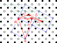
Figure 2: Remapping of atomic positions in the primitive and non-primitive descriptions, shown for one particular $\bullet$ $(m=2)$ of the two dimensional crystal of Fig. 1. Primary motif corresponds to Fig. 1(c). Thin dashed and solid lines show a few primitive and non-primitive cells respectively. Bonds between $\circ$ and $\bullet$ not shown, for clarity.

In order to simplify $\Lambda$, we point out that (18) implies $Im(\bm{k_{\theta}}^{\perp})=Im(\bm{K}^{\perp})$. Hence $\alpha=2Im(\bm{K}^{\perp}\cdot\bm{f}_{1})=L_{1}\times 2Im(\bm{k_{\theta}}^{\perp}\cdot\bm{u}_{1})=L_{1}\beta$. Also note that $M_{1}=L_{1}N_{1}$. Thus, from (16), (36) we have

$$\Lambda=\cases{1,&if $\alpha=\beta=0$,\\ \sqrt{L_{1}\frac{1-e^{-\beta}}{1-e^{-\alpha}}},&if $\alpha,\beta\neq 0$ .}$$ (25)

It is important to appreciate that our choices of $M_{1}=L_{1}N_{1}$ and summation limits for $t,s$ in (14), (34) ensure that though $S_{NP},S_{P}\to\infty$ as $N_{1},M_{1}\to\infty$ and $\alpha,\beta<0$, the ratio $\frac{S_{NP}}{S_{P}}$ is always well behaved.

We can transform (23) into a matrix equation,

$$[B_{\mu\varsigma m}] = \Lambda\;[U]\cdot[A_{\mu\varsigma m}]$$ (26)

where

$${[B_{\mu\varsigma m}]}= \left[\begin{array}[]{c}e^{-\iota\bm{K}\cdot\bm{w}_{1}}\tilde{C}^{\prime\;\mu\varsigma m1}(\bm{K}^{\perp})\\ \vdots\\ e^{-\iota\bm{K}\cdot\bm{w}_{\mathcal{N}_{c}}}\tilde{C}^{\prime\;\mu\varsigma m\mathcal{N}_{c}}(\bm{K}^{\perp})\end{array}\right],$$

$${[U]}=\frac{1}{\sqrt{\mathcal{N}_{c}}} \left[\begin{array}[]{ccc}e^{\iota\bm{w}_{1}\cdot\bm{q}_{1}}&\cdots&e^{\iota\bm{w}_{1}\cdot\bm{q}_{\mathcal{N}_{c}}}\\ \vdots&\ddots&\vdots\\ e^{\iota\bm{w}_{\mathcal{N}_{c}}\cdot\bm{q}_{1}}&\cdots&e^{\iota\bm{w}_{\mathcal{N}_{c}}\cdot\bm{q}_{\mathcal{N}_{c}}}\\ \end{array}\right],$$

$${[A_{\mu\varsigma m}}]= \left[\begin{array}[]{c}a_{1}\tilde{c}^{\prime\;\mu\varsigma m}((\bm{K}+\bm{q}_{1})^{\perp})\\ \vdots\\ a_{\mathcal{N}_{c}}\tilde{c}^{\prime\;\mu\varsigma m}((\bm{K}+\bm{q}_{\mathcal{N}_{c}})^{\perp})\end{array}\right].$$

We remark that (26) is very similar to the equation derived in [10] for the case of real bands, except for the additional factor $\Lambda$. Following [10], we solve (26) to obtain $[A_{\mu\varsigma m}]$ for all combinations of $\mu\varsigma m$, using the property that $[U]$ is unitary. Since we have ensured $\sum_{\mu\varsigma m}|\tilde{c}^{\prime\;\mu\varsigma m}|^{2}=1$, we obtain

$$a_{\theta}=\sqrt{\sum_{\mu\varsigma m}{\Big{|}[A_{\mu\varsigma m}]_{\theta}\Big{|}}^{2}}$$ (30)

Further, since both $|{\Psi(\bm{K})}\rangle$ and $|{\psi(\bm{k})}\rangle$ have been normalized, and wavefunctions corresponding to different wavevectors are orthogonal, the measure associated with the projections of the non-primitive wavefunction $|{\Psi(\bm{K})}\rangle$ onto candidate primitive wavefunctions $|{\psi(\bm{K}+\bm{q}_{\theta})}\rangle$,

$$\mathcal{M}=\sum_{\theta=1}^{\mathcal{N}_{c}}|a_{\theta}|^{2}=1,$$ (31)

independent of the energy $E$. It is reasonable to expect that most $a_{\theta}$ will be zero. The primitive wavevectors $\bm{K}+\bm{q}_{\theta}$ ($\forall\theta$ such that $a_{\theta}\neq 0$) represent unfolded states corresponding to the non-primitive wavevector $\bm{K}$. Note that these may lie outside the first primitive Brillouin zone, in which case, they need to be shifted back in using an appropriate primitive reciprocal lattice vector.

We now clarify an issue related to determining the values of $\tilde{C}^{\prime\mu\varsigma n}$ from the eigenvectors of the non-primitive version of palindromic eigenvalue problem (5). Note first that $\mathtt{constant}\times[C_{t}]$ is as good an eigenvector as $[C_{t}]$, where $\mathtt{constant}$ is in any complex number independent of $\mu\varsigma n$. Thus, the eigensolver can be thought of as returning an eigenvector, $\mathtt{constant}\times[C_{t}]$, normalized such that $\sum_{\mu\varsigma n}|\mathtt{constant}\times[C_{t}]_{\mu\varsigma n}|^{2}=1$. Now, from (12), (13) we have

$$\tilde{C}^{\prime\mu\varsigma n}(\bm{K}^{\perp})=e^{\iota\bm{K}^{\parallel}\cdot\bm{\gamma}_{n}}\times\underbrace{\sqrt{S_{NP}(\bm{K}^{\perp})}e^{-\iota\bm{K}^{\perp}\cdot t\bm{f}_{1}}\times[C_{t}]_{\mu\varsigma n}}_{\mathrm{eigenvector}}$$ (32)

Choosing $\mathtt{constant}=\sqrt{S_{NP}(\bm{K}^{\perp})}e^{-\iota\bm{K}^{\perp}\cdot t\bm{f}_{1}}$, we can associate $\tilde{C}^{\prime\mu\varsigma n}$ with the eigenvector returned by the solver, after scaling individual rows are by $e^{\iota\bm{K}^{\parallel}\cdot\bm{\gamma}_{n}}$, as shown in (32). Since $\bm{K}^{\parallel}$ is real, this ensures that $\sum_{\mu\varsigma n}|\tilde{C}^{\prime\;\mu\varsigma n}|^{2}=1$.

Finally, a we would like to comment on the possible implications of this work to determine the complex bandstructure of disordered materials. The supercell method computes energy bands using a large non-primitive supercell, and unfolds these onto a fictitious primitive small-cell. This supercell is non-primitive w.r.t $\bm{u}_{2},\bm{u}_{3}$ (i.e. $\bm{f}_{2}=N_{2}\bm{u}_{2},\bm{f}_{3}=N_{3}\bm{u}_{3}$ for integers $N_{2},N_{3}>1$). As mentioned earlier, a careful choice of linearization scheme and eigensolver is essential to obtain useful results. Systems with disorder can be thought to have a spread in their $E(\bm{k})$ dispersion – i.e. at any $\bm{k}$, there are states with energies within an interval given by a mean energy $\bar{E}$, and a deviation $\delta E$ about this mean. Equivalently, at any energy $E$, each complex band can be thought of having a mean $\bar{\bm{k}}^{\perp}(E)$ and a spread $\delta\bm{k}^{\perp}(E)$. The central idea of the supercell technique applied to real bands is to extend the summation in (20) so that a supercell state $|{\Psi_{p}(\bm{K})}\rangle$ with energy $E_{p}$ is expressed in terms of $N_{O\,cell}$ small cell states with energies $E_{\eta}$ as

$$|{\Psi_{p}(\bm{K})}\rangle=\sum_{\eta=1}^{N_{O\,cell}}\sum_{\theta=1}^{\mathcal{N}_{c}}a_{\eta,\theta;p}|{\psi_{\eta}(\bm{K}+\bm{q}_{\theta})}\rangle,$$ (33)

where $N_{O\,cell}$ refers to the number of orbitals in the small-cell, and hence is the number of small-cell energy bands at any given $\bm{k}$. It is reasonable to expect that the supercell technique, when extended to compute the complex bandstructure of disordered materials will similarly involve a summation of states with different energies. The invariance of $\mathcal{M}$ on energy will hence be useful in simplifying computation. The details of such a computation are beyond the scope of the present work, and could be the subject of further study.

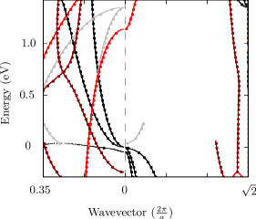
Figure 3: Complex bandstructure of Silicon (lattice constant $a$) along $[110]$. Tight binding parameters are taken from [5]. Real and imaginary parts of the wavevector are shown on the right and left panels respectively. Pure real and pure imaginary bands are in black, red whereas complex bands are in grey, dark red for $\bm{k}^{\parallel}=\bm{0}$, $\bm{k}^{\parallel}=(0,0,0.84\times 2\pi/a)$ respectively. Lines represent results using primitive vectors whereas the filled squares represent results using non-primitive vectors followed by zone unfolding.

4 Application and Summary

Transport along the $[110]$ direction leads to a quartic GPEP when working with primitive vectors. On the other hand, the smallest non-primitive unit cell such that $\bm{f}_{1}\parallel\bm{n}$ is a double cell ($\mathcal{N}_{c}=2$). Thus, there are two possible primitive wavevectors that each non-primitive wavevector can unfold onto. Figure 3 compares the complex bandstructure of Silicon along the $[110]$ direction, obtained using a primitive cell with that obtained using this non-primitive cell, followed by our zone-unfolding procedure. Tight binding parameters are taken from [5]. Two different value of $\bm{k}^{\parallel}$ are considered, corresponding to $\bm{k}$ paths through $(0,0,0)$ (valence band maximum) and $(0,0,0.84\times 2\pi/a)$ (one of the $\Delta$ conduction valleys). The two methods yield identical results. Further, Table 1 demonstrates the invariance of the measure $\mathcal{M}=\sum_{\theta}|a_{\theta}|^{2}$ on energy $E$ ensured by the inclusion of the factor $\Lambda$.

In conclusion, we have derived a unified method of unfolding real and complex bands in a nearest neighbour tight-binding scheme. This method reduces to the unfolding method available in literature [10], for the case of real bands. Using this unfolding method, complex bands along any general transport direction $\bm{n}$ can be computed by the solution of a generalized quadratic eigenvalue problem, using a non-primitive unit cell. This overcomes the difficulties regarding the solution of generalized polynomial eigenvalue problems of large order, that may result when computing complex bands using primitive cells for general $\bm{n}$. Finally, our method ensures an energy invariant measure for the projections of the non-primary wavefunction onto all candidate primary wavefunctions. This invariance will be important for computing complex bands of disordered materials using a supercell approach [12].

Table 1: Effect of factor $\Lambda$ (26) on the measure $\mathcal{M}=\sum_{\theta}|a_{\theta}|^{2}$ for states having the smallest values of $|Im(k^{\perp}(E))|$ and $\bm{k}^{\parallel}=(0,0,0.84\times 2\pi/a)$. $\mathcal{M}_{old}$ is the value of $\mathcal{M}$ setting $\Lambda=1$, corresponding to the result provided by the real band unfolding algorithm of [10]. $\mathcal{M}_{new}$ corresponds to the measure as computed by the modified unfolding algorithm described in this work.

• $E\;(eV)$	$K^{\perp}\;(2\pi/a)$	$k^{\perp}\;(2\pi/a)$	$\mathcal{M}_{old}$	$\mathcal{M}_{new}$
  $0.05$	$-0.116+0.126\iota$	$1.299+0.126\iota$	$1.272$	$1.0$
  $0.8$	$0.103\iota$	$0.103\iota$	$1.224$	$1.0$

Appendix

Appendix A Primitive wavefunction in terms of atomic orbitals

Replacing $\bm{f},t,\bm{R},n,N,\Xi,\Psi,C^{\prime}$ describing the non-primitive wavefunctions with $\bm{u},s,\bm{\rho},m,M,\xi,\psi,c^{\prime}$ respectively in Section 3.1, we have the primary wavefunction

$$|{\psi(\bm{k}^{\perp},\bm{k}^{\parallel})}\rangle=\frac{1}{\sqrt{M_{\parallel}S_{P}(\bm{k}^{\perp})}}\sum_{\mu\varsigma m}\sum_{j}^{(M_{\parallel})} \sum_{s=0}^{M_{1}-1}\tilde{c}^{\prime\;\mu\varsigma m}(\bm{k}^{\perp})\times$$ (34)

$$e^{\iota\bm{k}^{\perp}\cdot s\bm{u}_{1}}e^{\iota\bm{k}^{\parallel}\cdot(\bm{\rho}^{\parallel}_{j}+s\bm{u}_{1})}|{\mu,\varsigma;\bm{\rho}^{\parallel}_{j}+s\bm{u}_{1}+\bm{\nu}_{m}}\rangle$$

In going from (34) to (17), we use the fact that by construction , $\bm{k}^{\perp}\cdot\bm{\rho}^{\parallel}_{j}=0$. Hence, the exponent in (34) is simplified as

$$\bm{k}^{\perp}\cdot s\bm{u}_{1}+\bm{k}^{\parallel}\cdot(\bm{\rho}^{\parallel}_{j}+s\bm{u}_{1})=\bm{k}\cdot\bm{\rho}_{j^{\prime}},$$ (35)

where $\bm{\rho}_{j^{\prime}}=(\bm{\rho}^{\parallel}_{j}+s\bm{u}_{1})$. The double summation in (34), $\sum_{j}^{(M_{\parallel})}\sum_{s=0}^{M_{1}-1}\equiv\sum_{j^{\prime}}^{(\mathcal{N}_{P})}$ (where $\mathcal{N}_{P}=M_{\parallel}M_{1}$ refers to the number of primitive lattice points) and the ^′ can finally be dropped from $j^{\prime}$.

Imposing the conditions that $\langle{\psi(\bm{k}^{\perp},\bm{k}^{\parallel})}|{\psi(\bm{k}^{\perp},\bm{k}^{\parallel})}\rangle=1$ and $\sum_{\mu\varsigma m}|\tilde{c}^{\prime\;\mu\varsigma m}(\bm{k}^{\perp})|^{2}=1$, we get

$$S_{P}(\bm{k}^{\perp}) = \sum_{s=0}^{M_{1}-1}e^{-s\beta},\mbox{ where }\beta=2Im(\bm{k}^{\perp}\cdot\bm{u}_{1})$$ (36)

$$= \cases{M_{1},&if $\beta=0$\\ \frac{1-e^{-\beta M_{1}}}{1-e^{-\beta}},&if $\beta\neq 0.$}$$

References

References

- [1] Kane E O 1961 J. Appl. Phys. 32 83
- [2] Tersoff J 1984 Phys. Rev. Lett. 52 465–468
- [3] Tersoff J 1984 Phys. Rev. B 30 4874–4877
- [4] Jancu J M, Scholz R, Beltram F and Bassani F 1998 Phys. Rev. B 57 6493–6507
- [5] Boykin T B, Klimeck G and Oyafuso F 2004 Phys. Rev. B 69 115201
- [6] Boykin T B 1996 Phys. Rev. B 54 8107–8115
- [7] Ajoy A, Murali K, Karmalkar S and Laux S 2011 Orientation dependent complex bandstructure of SiGe alloys Device Research Conference (DRC), 2011 69th Annual pp 113 –114
- [8] Mackey D, Mackey N, Mehl C and Mehrmann V 2007 SIAM J. Matrix Anal. Appl. 28 1029–1051
- [9] Laux S E 2009 Computation of Complex Band Structures in Bulk and Confined Structures Computational Electronics, 2009. IWCE’09. 13th International Workshop on (IEEE) pp 1–2
- [10] Boykin T and Klimeck G 2005 Phys. Rev. B 71 115215
- [11] Boykin T B, Kharche N and Klimeck G 2006 Eur. J. Phys. 27 5–10
- [12] Boykin T B, Kharche N, Klimeck G and Korkusinski M 2007 J. Phys. : Condens. Matter 19 036203
- [13] Boykin T, Kharche N and Klimeck G 2007 Phys. Rev. B 76 035310
- [14] Boykin T, Kharche N and Klimeck G 2009 Physica E 41 490–494
- [15] Ku W, Berlijn T and Lee C 2010 Phys. Rev. Lett. 104 216401
- [16] Slater J and Koster G 1954 Phys. Rev. 94 1498
- [17] Aravind P 2006 Am. J. Phys. 74 794
- [18] Löwdin P 1950 J. Chem. Phys. 18 365
- [19] Ipsen I 2004 SIAM News 37 1–2
- [20] Mackey D, Mackey N, Mehl C and Mehrmann V 2006 SIAM. J. Matrix Anal. & Appl. 28 971
- [21] Huang T, Lin W and Su W 2011 Numerische Mathematik 1–23