Constraints on ionising photon production from the large-scale Lyman-alpha forest

Abstract

Recent work has shown that the $z\simeq 2.5$ Lyman-alpha forest on large scales encodes information about the galaxy and quasar populations that keep the intergalactic medium photoionized. We present the first forecasts for constraining the populations with data from current and next-generation surveys. At a minimum the forest should tell us whether galaxies or, conversely, quasars dominate the photon production. The number density and clustering strength of the ionising sources might be estimated to sub-$10\%$ precision with a DESI-like survey if degeneracies (e.g., with the photon mean-free-path, small-scale clustering power normalization and potentially other astrophysical effects) can be broken by prior information. We demonstrate that, when inhomogeneous ionisation is correctly handled, constraints on dark energy do not degrade.

1. Introduction

Almost fifty years after Gunn & Peterson (1965) first used quasar spectra to infer the intergalactic neutral hydrogen density, the Lyman-$\alpha$ forest remains a key probe of cosmological physics. The forest has been widely used to measure small-scale structure (e.g., Croft et al., 1999; McDonald et al., 2006) and more recently datasets of tens of thousands of spectra have allowed us to correlate cosmic density over tens to hundreds of megaparsecs (McDonald, 2003; McQuinn & White, 2011; Slosar et al., 2011). This opens up the possibility of constraining the expansion history – and so dark energy – by measuring the scale of the baryon acoustic oscillations (BAO) (McDonald & Eisenstein, 2007; Busca et al., 2013; Slosar et al., 2013; Delubac et al., 2014). But there is more information to be harvested given a sufficiently accurate measurement of the Lyman-$\alpha$ correlation function. The possibility that astrophysics distorts cosmological correlation functions has been foreseen for some time (e.g., Bower et al., 1993) but concrete processes have typically been studied only over quite small patches of a few megaparsecs (e.g., Kollmeier et al., 2003; Meiksin & White, 2004). We focus here on a correction to fluctuations in patches of size tens to hundreds of megaparsecs, arising from a radiation effect that increases in amplitude as the scales become comparable to the mean free path of an ionising photon (Croft, 2004; McDonald et al., 2005; McQuinn et al., 2011b; Pontzen, 2014; Gontcho et al., 2014). We will use the description of Pontzen (2014, henceforth P14) to demonstrate that one can constrain the nature of ionising radiation sources in the redshift range $2<z<3$, provided that various calibration uncertainties are under control.

The underlying physical process is an analogue of the proximity effect (e.g., Murdoch et al., 1986; Bajtlik et al., 1988; Dall’Aglio et al., 2008; Calverley et al., 2011) – in regions of high ultraviolet (UV) photon density, the forest is suppressed because the neutral fraction of hydrogen declines. But while the classical proximity effect applies in the relatively small, several-megaparsec region where a single nearby quasar appreciably boosts the UV background, the process here arises due to averaged fluctuations in emissivity over much larger scales. The finite mean free path dictates that ionising radiation cannot reach uniformity in patches larger than a few hundred comoving megaparsecs; if one probes Hi fluctuations on scales approaching this limit, there are unavoidable distortions in the power spectrum.

The P14 analysis solves the Boltzmann radiative transfer equation by assuming that the radiation field is in local equilibrium, and that the equations can be linearized by averaging over small scales. The result is a quantitative link between the power spectrum of Hi fluctuations ($P_{\mathrm{HI}}(k)$) and that of the total density ($P(k)$), dependent on a number of astrophysical parameters. These include the bias of UV sources, $b_{j}$; the number density of UV sources, $\bar{n}$; and the opacity of the intergalactic medium to Lyman-limit (i.e., ionising) radiation, $\kappa_{\mathrm{HI}}$. When multiple populations contribute, $b_{j}$ and $\bar{n}$ average in well-defined ways. As a reference model, we will adopt the P14 default parameter values: $b_{j}\simeq 3$, $\bar{n}\simeq 10^{-4}\,h^{3}\,\mathrm{Mpc}^{-3}$ and $\kappa_{\mathrm{HI}}\simeq(390\,h^{-1}\,\mathrm{Mpc})^{-1}$.

The detailed calculation given by P14 reveals that, even though source clustering is weak over the vast distances involved, radiative transfer generates a major correction to the expected power spectrum because the clustering of the gas is weaker still. Shot noise is also a major factor: the rarity of sources, again a small effect on such scales, can still be significant compared to the tiny cosmological clustering power. These results are reinforced by an alternative calculation by Gontcho et al. (2014). There are, however, potential complications arising from temperature fluctuations. These impact on the flux transmission by modifying the neutral fraction and by changing the shape of a cloud’s absorption profile; they were not included in the analysis of P14, but an estimate by Gontcho et al. (2014) showed them to generate only a small correction to the power spectrum. We therefore continue to ignore them for our exploratory work here (but see Section 5).

2. Correlation functions and their parameters

To make forecasts for future forest analyses, we constructed a pipeline based on the BOSS (Baryon Oscillation Spectroscopic Survey) approach as described by Busca et al. (2013, henceforth B13). While P14 gives a prediction for the linear Hi power spectrum, $P_{\mathrm{HI}}(k)$, here we need the Lyman-alpha transmission flux power spectrum $P_{F}(k)$. We consider only scales that are far above the non-linear dynamics regime; on the other hand the non-linear effects on small scales still cannot be entirely neglected (e.g., McDonald et al., 2000; McDonald, 2003; Seljak, 2012). In particular spatial averaging does not commute with the transformation to flux, and our $P_{\mathrm{HI}}(k)$ therefore cannot simply be rescaled. Instead one must decompose the processes shaping $P_{\mathrm{HI}}(k)$ back into their separate physical origins and reassemble them in an appropriate way as we now describe. This process will also introduce angle-dependence from redshift-space distortions (Kaiser, 1987; Hamilton, 1998).

In the absence of radiation fluctuations one has two parameters: a density bias $b_{F}$ and a velocity bias $b_{Fv}$. These relate changes in the large-scale average flux field to the linear fractional overdensity field $\delta_{\rho}$ by

$$\delta_{F}=\left[b_{F}+(1+\mu^{2})b_{Fv}\right]\delta_{\rho}\textrm{,}$$ (1)

where $\delta_{A}=A(\mathbf{x})/\langle A\rangle-1$ for any field $A$, and $\mu$ is the cosine of the angle to the line-of-sight. The dependence of the redshift-space distortions on cosmology has been neglected since we are working at high redshift (Hamilton, 1998). From simulations (e.g., McDonald, 2003) one has $b_{F}\simeq-0.14$ and $b_{Fv}\simeq-0.20$, compatible with the observational constraint on $b_{F}+b_{Fv}\simeq-0.34$ (Slosar et al., 2011).

When we introduce inhomogeneous radiation, a further term must be added:

$$\delta_{F}=\left[b_{F}+(1+\mu^{2})b_{Fv}\right]\delta_{\rho}+b_{F\Gamma}\delta_{\Gamma}\textrm{,}$$ (2)

where $\delta_{\Gamma}$ are the fractional fluctuations in the ionisation rate and $b_{F\Gamma}$ is a new bias parameter describing the response of the flux. The redshift space distortions, being gravitational in origin, are unaffected by inhomogeneous radiation at first order ($b_{Fv}$ is unchanged). A numerical value of $b_{F\Gamma}$ is determined by averaging over the response of individual Lyman-$\alpha$ lines to an increase in Hi fraction (Font-Ribera et al., 2013), giving $b_{F\Gamma}\simeq 0.13$ (Font-Ribera et al., 2013; Gontcho et al., 2014). We also verified this result using the simulations of Bird et al. (2011).

The radiation fluctuations correlate with the cosmic density so that in Fourier space

$$\langle\delta_{\Gamma}(k)\delta_{\rho}(k)\rangle\propto b_{\Gamma\rho}(k)P(k)\textrm{,}$$ (3)

where $b_{\Gamma\rho}(k)$ is the scale-dependent bias describing the relationship between radiation and $P(k)$, the underlying cosmological power spectrum. The bias $b_{\Gamma\rho}(k)$ encodes the radiative transfer physics and scales near-linearly with the source clustering strength $b_{j}$ [in P14 $b_{\Gamma\rho}(k)$ is given by equation (35) since $b_{\mathrm{HI}}(k)=b_{\mathrm{HI,u}}-b_{\Gamma\rho}(k)$ in the notation there]. An additional, uncorrelated shot noise contribution enters so that

$$\langle\delta_{\Gamma}(k)\delta_{\Gamma}(k)\rangle\propto b_{\Gamma\rho}(k)^{2}P(k)+N(k)\textrm{.}$$ (4)

The scale-dependence of $N(k)$ is specified by the radiation transfer physics [corresponding to the second term in equation (38) of P14]; its amplitude is inversely proportional to the number density $\bar{n}$ of sources.

Combining the equations above, the flux power spectrum is

$$P_{F}(k,\mu)=\left[b_{F}+(1+\mu^{2})b_{Fv}+b_{F\Gamma}b_{\Gamma\rho}(k)\right]^{2}P(k)+b_{F\Gamma}^{2}N(k)\textrm{.}$$ (5)

Current analyses of the forest measure the correlation function $\xi_{F}(r,\mu)=\langle\delta_{F}(\mathbf{x})\delta_{F}(\mathbf{x}+\mathbf{r})\rangle$, where $\mu$ is the angle between the displacement vector $\mathbf{r}$ and the line of sight. This contains equivalent information to the power spectrum $P_{F}(k,\mu)$ and is related by decomposing the angular dependence into Legendre polynomials:

$$P_{F}(k,\mu)=\sum_{\ell=0,2,4}P_{F,\ell}(k)p_{\ell}(\mu)\textrm{;}\hskip 5.69046pt\xi_{F}(r,\mu)=\sum_{\ell=0,2,4}\xi_{F,\ell}(r)p_{\ell}(\mu)\textrm{,}$$ (6)

where $p_{\ell}$ is the Legendre polynomial of order $\ell$. (The linear-order Kaiser 1987 approximation only generates terms with $\ell=0,2$ and $4$.) Calculating the moments of the power spectrum $P_{F,\ell}(k)$ is a matter of rewriting the $\mu$-dependence of (5) in terms of the $p_{\ell}$’s. The final step is to relate $\xi_{F,\ell}$ to $P_{F,\ell}$; one may show that

$$\xi_{F,\ell}(r)=\frac{i^{\ell}}{2\pi^{2}}\int_{0}^{\infty}\mathrm{d}k\,k^{2}P_{F,\ell}(k)j_{\ell}(kr)\textrm{,}$$ (7)

where $j_{\ell}$ is the spherical Bessel function of order $\ell$ (Hamilton, 1998). Following B13 we will work directly with the multipoles. An example of $\xi_{F,0}$ and $\xi_{F,2}$ is shown in Figure 1 for our standard parameters (solid line) and the equivalent model with a completely uniform UV background (dashed line). Cosmological parameters are unchanged from P14 and based on Planck Collaboration (2013); the underlying power spectrum is calculated with CAMB (Lewis et al., 2000).

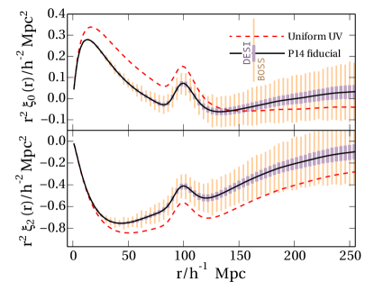
Figure 1.— The first two multipole moments of the redshift-space flux correlation function $\xi_{0}$ and $\xi_{2}$; the dashed line corresponds to a uniform UV background, and the solid line to the P14 solution with UV from a mix of quasars and galaxies. As the dominant sources change from galaxies to quasars, the solution moves further away from the uniform limit (see figures 3 to 5 in P14). The thick and thin error bars show respectively the diagonal part of the covariance for DESI and BOSS. Correlation of the errors is $\simeq 20\%$ between neighbouring measurements.

The Lyman-$\alpha$ forest constrains the angular diameter distance and Hubble parameters via the transverse and line-of-sight BAO. Current analyses (e.g., B13) assume a fiducial cosmology during an initial conversion from raw data to the correlation function, then measure departures of the BAO feature from its expected location. We therefore decompose all our power spectra into two parts, a ‘smooth’ and a BAO ‘peak’ component, following the recipe given by Kirkby et al. (2013). The peak component is then shifted in scale by a fixed factor $\alpha$; for $\alpha=1$, one recovers the exact fiducial cosmology. If one fixes the transfer function, the forest encodes further information on the spectral index of primordial fluctuations $n_{s}$; we add another proxy cosmological parameter, $\zeta$, such that

$$P_{F}(k)\to P_{F}(k)\left(\frac{k}{0.1\,h^{-1}\,\mathrm{Mpc}}\right)^{\zeta-1}\textrm{.}$$ (8)

This definition returns the default cosmology when $\zeta=1$ and pivots around the arbitrary scale $0.1\,h^{-1}\,\mathrm{Mpc}$. In a realistic case $\zeta$ will constrain a degenerate combination of $n_{s}$ and cosmic density parameters.

	Cosmological parameters
$\alpha$	Scaling of the BAO peak position
$\zeta$	Broadband spectral tilt $=n_{s}$ if transfer function is fixed
	Astrophysical parameters (scale-independent)
$b_{j}$	Bias of UV sources (weighted average)
$\bar{n}$	Number density of UV sources (weighted average)
$\kappa_{\mathrm{HI}}$	Opacity of the intergalactic medium to ionising radiation
$b_{\mathrm{HI,u}}$	Bias of intergalactic Hi ignoring UV fluctuations
	Astrophysical functions (scale-dependent)
$b_{\Gamma\rho}(k)$	Bias of UV fluctuations, depends on $b_{j}$ and $\kappa_{\mathrm{HI}}$
$N(k)$	Noise from UV fluctuations, depends on $\bar{n}$ and $\kappa_{\mathrm{HI}}$
$b_{\mathrm{HI}}(k)$	= $b_{\mathrm{HI,u}}-b_{\Gamma\rho}(k)$; overall bias of intergalactic Hi
	Forest parameters (scale-independent)
$b_{F}$	Bias of the observed forest (ignoring UV and velocity)
$b_{Fv}$	Bias of the observed forest relative to redshift-space distortions
$b_{F\Gamma}$	Bias of the observed forest relative to UV intensity
	Nuisance parameters
$a_{\ell,n}$	Six flux-calibration broadband distortion parameters

Table 1A reference guide for the quantities used in this Letter.

Finally, following B13, we introduce nuisance parameters to characterise distortions induced by current pipelines:

$$\xi_{F,\ell}\to\xi_{F,\ell}+\sum_{n=0}^{2}a_{\ell,n}r^{-n}\textrm{.}$$ (9)

These have been shown by use of mocks to be an adequate description of uncertainty from quasar continuum estimates relying on data in the region of the forest (Kirkby et al., 2013, B13).

3. Statistical techniques and cosmological biases

We constructed covariance matrices $\mathsf{C}$ summarising the expected noise properties of two separate survey configurations. We considered only those data lying in the redshift range $2<z<3$; the two major parameters are then the number of quasars $N_{\mathrm{QSO},z}$ in this redshift range and the sky coverage area $A$. We refer to our covariances as BOSS, corresponding to the final planned data release ($N_{\mathrm{QSO},z}=1.5\times 10^{5}$, $A=10\,000$ sq. deg.: Dawson et al. 2013); and DESI, referring to a futuristic survey modelled on the Dark Energy Spectroscopic Instrument ($N_{\mathrm{QSO},z}=7.5\times 10^{5}$, $A=14\,000$ sq. deg.: Levi et al. 2013). We made use of the recipe given by B13 to generate the diagonal and leading-order off-diagonal terms from an estimation of $N_{\mathrm{pair}}$, the number of survey pixels separated by a given spatial distance. This will be a reasonable approximation independent of cosmology (since the dominant terms arise from one-point variance related to local, rather than large-scale, structure) and independent of survey (because the target signal-to-noise is similar for BOSS and DESI). These considerations also explain why the covariance matrix is near-diagonal. To verify our $N_{\mathrm{pair}}$ estimation procedure we emulated BOSS-DR9, based on numbers quoted in B13 ($N_{\mathrm{QSO},z}=4.8\times 10^{4}$, $A=3\,300$ square degrees) and verified that our estimated covariance matrix very closely mimics the published bootstrap estimation by B13.

Results will be quoted using only separation scales larger than $40\,h^{-1}\,\mathrm{Mpc}$, to ensure that the linear approximations of P14 hold (i.e., that local non-linear physics is safely segregated in constants such as $b_{\mathrm{HI,u}}$, $b_{v}$ and $b_{F\Gamma}$). We assumed uniform priors on all parameters and adopted a Gaussian likelihood approximation, equivalent to B13’s use of $\chi^{2}$ statistics.

Figure 2.— (Left panel) the forecast relative errors (i.e., the rms deviation divided by the mean) for simultaneously constraining all parameters with BOSS or DESI-like surveys. See Table 1 for an explanation of each variable. With BOSS ($+$ symbols) and DESI ($\diamond$ symbols) one can derive significant constraints on $b_{j}$ and $\bar{n}$ which describe the origin of UV photons, although these are weaker if the intergalactic medium opacity $\kappa_{\mathrm{HI}}$ is assumed unknown ($\times$ symbols). Traction on the astrophysics is lost if the continuum-induced broadband distortions are not adequately characterised ($\circ$ symbols). (Right panel) the correlation matrix for DESI-like case shows that the error budget for $b_{j}$ and $\bar{n}$ arises largely from a degeneracy with $\kappa_{\mathrm{HI}}$, explaining the major difference between $\times$ and $\diamond$ cases in the left panel.

We first investigated whether cosmological parameter estimation may be biased by the inhomogeneous radiation. This is a matter of generating mock data using our fiducial UV solution, but attempting to fit the results without any radiative distortions (i.e., with $b_{F\Gamma}=0$), leaving the nuisance parameters $a_{\ell,n}$ to mop up the resulting broadband distortion. Current pipelines closely recover the BAO peak position despite the unmodeled effects. In particular using the BOSS covariance matrix, we found $\alpha=1.004\pm 0.025$ where the central value is the marginalized mean over the posterior and the error is its standard deviation. For DESI, we obtained $\alpha=1.003\pm 0.005$.

These expected systematic errors are significantly smaller than the $1\%$ shift in the BAO peak reported in P14 for two reasons: first, much of the observed signal comes from the redshift space distortions (which are not subject to radiative effects). Second, P14 directly measured the position of the peak, whereas here we marginalized over a generic set of broadband distortions $a_{\ell,n}$ which partially remove the shape modulation.

Consequently the expected biases are an order-of-magnitude too small to account for a several-percent level tension with $\Lambda$CDM reported by Delubac et al. (2014). Even if one substantially increases the size of the modulation, for instance by reducing $\bar{n}$ or increasing $b_{j}$, the $a_{\ell,n}$-fitting restricts the errors to below one percent. On the other hand with future surveys this decoupling may not be sufficient – for example with DESI and $b_{j}=4$ (reflecting a large quasar contribution) we find $\alpha=1.006\pm 0.006$, which starts to be problematic.

Errors can be reduced by implementing a more flexible broadband distortion function; or they can be eliminated by fitting astrophysical parameters. The latter approach delivers insight into the galaxy and quasar population, as we now discuss.

4. Astrophysical forecasts

We use a Fisher matrix formalism (see, e.g., Albrecht et al., 2006) to estimate the covariance matrix for maximum likelihood parameter estimates, determining how accurately astrophysical and cosmological parameters can be inferred. Figure 2 shows the results for simultaneously fitting seven key parameters from Section 2 (see Table 1). In the left panel we show the diagonal elements of the Fisher matrix divided by the true value of the parameter: this gives a prediction for the $1\sigma$ relative error for a given quantity, marginalized over the other six parameters. The different point styles represent different scenarios described below.

Consider the most optimistic scenario – a DESI-like survey with accurate broadband characterisation, plus a known intergalactic medium optical depth $\kappa_{\mathrm{HI}}$ to ionising photons ($\diamond$ symbols, left panel of Figure 2). In this case, one obtains a constraint on $b_{j}$, the clustering bias of UV sources, and on $\bar{n}$, the number density of such sources, both accurate to around $4\%$. We could then easily infer whether ionising photons at $z\sim 2.5$ are typically produced by galaxies, quasars or both. This does assume that the calibration of $b_{F\Gamma}$ is perfect, but given close agreement between simulations and generic analytic arguments (Section 2), such an assumption is warranted.

There is currently disagreement over the precise photon mean free path (e.g., Rudie et al., 2013; Prochaska et al., 2014), so one might allow $\kappa_{\mathrm{HI}}$ to float. In this scenario, constraints on $b_{j}$ and $\bar{n}$ degrade significantly (see $\times$ symbols in Figure 2) to $20\%$ errors on $b_{j}$ and $\simeq 60\%$ errors on $\bar{n}$. The right panel of Figure 2 shows degeneracies between the parameters for this case, illustrating why advance knowledge is so helpful: there is a near-complete three-way degeneracy between $\kappa_{\mathrm{HI}}$, $\bar{n}$ and $b_{j}$. Increasing $\kappa_{\mathrm{HI}}$ brings the effects of radiative transfer to smaller scales; this can be counterbalanced by increasing the number density and reducing the clustering of the sources. However a weak prior on $\kappa_{\mathrm{HI}}$ is sufficient to break the degeneracy; for example, taking a $\kappa_{\mathrm{HI}}$ prior with standard deviation $\pm 20\%$, the forest gives estimates accurate to $7\%$ ($b_{j}$) and $22\%$ ($\bar{n}$).

In the left panel of Figure 2 we have also plotted (as $+$ symbols) the forecasts for BOSS. One obtains $\sim 15\%$ constraints on $b_{j}$ and $\bar{n}$; all the above caveats apply, in that one needs a reasonable prior on $\kappa_{\mathrm{HI}}$ to achieve this. The uppermost line (with $\circ$ symbols) shows BOSS constraints marginalized over an unknown broadband distortion, which the current pipelines require; floating the distortion parameters $a_{\ell,n}$ implies loss of traction on the astrophysics. In other words the astrophysical information is lost unless the broadband shape of $\xi_{F}$ can be reconstructed accurately. Robust methods to calibrate the quasar continuum are therefore required (e.g., Pâris et al., 2011; Lee, 2012).

We found that constraints on the BAO peak location are not degraded by marginalising over the astrophysical parameters we consider (compared against an ideal case where radiative distortions are fixed or artificially switched off). For instance $\alpha$, the BAO position, is constrained to $\pm 2.8\,\%$ with BOSS; we verified this is exactly the same constraint as obtained in the ideal, undistorted case. This applies to an isotropic rescaling, but different cosmological information is available from the rescaling along and perpendicular to the line of sight (Slosar et al., 2013; Delubac et al., 2014). When constraining these directions separately, anisotropic distortions can mix the moments of the correlation function so leading to broadband distortions. The main effect is to slightly degrade the astrophysical constraints. Taking the DESI case, for example, we find that the relative uncertainty on $b_{j}$ rises from $4\%$ with isotropic scaling to $6\%$ when the scaling along the two directions is independent.

5. Conclusions

We have investigated the potential of present and planned surveys of the large-scale Lyman-$\alpha$ forest to reveal properties of the objects producing ionising photons at $z\simeq 2.5$. We find that, provided pipelines can be developed where the broadband calibration distortions are largely eliminated or fully characterized, there are excellent prospects for deriving meaningful data on population number density $\bar{n}$ and clustering strength $b_{j}$. These constraints can in turn be used to discriminate between galaxy- and quasar-dominated scenarios; or compared against a more sophisticated model for the origin of photons in which $\bar{n}$ and $b_{j}$ become weighted population averages. Such an approach would be highly complementary to constructing luminosity functions for high-redshift galaxies and quasars, since it traces all emission rather than just that coming from the brightest objects – and automatically folds in the effect of varying escape fractions.

We have not yet investigated the additional power that would come from cross-correlation studies (e.g., Font-Ribera et al., 2013), nor have we investigated how splitting the results into redshift bins could give constraints on evolution. The results we have presented assume that the small-scale nonlinearities can be simulated well enough to consider the radiative flux bias $b_{F\Gamma}$ known, and that $\sigma_{8}$ can be derived from other datasets; without this calibration, one would instead have to estimate ratios such as $b_{j}/b_{\mathrm{HI,u}}$. We have ignored systematics such as residual metal-line contamination (Iršič & Slosar, 2014) and large-scale temperature fluctuations (McQuinn et al., 2011a; Gontcho et al., 2014). It is currently unclear to what extent these will be degenerate with each other and with the constraints we seek – a campaign of simulations and analytic work to understand how various effects and approximations interact with each other is required. But the basic result that astrophysics distorts the large scale forest fluctuations in useful, measurable ways will survive, even if the degeneracies are somewhat more complex than we can currently model.

References

- Albrecht et al. (2006) Albrecht, A., Bernstein, G., Cahn, R., et al. 2006, Report of the Dark Energy Task Force, astro-ph/0609591
- Bajtlik et al. (1988) Bajtlik, S., Duncan, R. C., & Ostriker, J. P. 1988, ApJ, 327, 570
- Bird et al. (2011) Bird, S., Peiris, H. V., Viel, M., & Verde, L. 2011, MNRAS, 413, 1717
- Bower et al. (1993) Bower, R. G., Coles, P., Frenk, C. S., & White, S. D. M. 1993, ApJ, 405, 403
- Busca et al. (2013) Busca, N. G., Delubac, T., Rich, J., et al. 2013, A&A, 552, A96
- Calverley et al. (2011) Calverley, A. P., Becker, G. D., Haehnelt, M. G., & Bolton, J. S. 2011, MNRAS, 412, 2543
- Croft (2004) Croft, R. A. C. 2004, ApJ, 610, 642
- Croft et al. (1999) Croft, R. A. C., Weinberg, D. H., Pettini, M., Hernquist, L., & Katz, N. 1999, ApJ, 520, 1
- Dall’Aglio et al. (2008) Dall’Aglio, A., Wisotzki, L., & Worseck, G. 2008, A&A, 491, 465
- Dawson et al. (2013) Dawson, K. S., Schlegel, D. J., Ahn, C. P., et al. 2013, AJ, 145, 10
- Delubac et al. (2014) Delubac, T., Bautista, J. E., Busca, N. G., et al. 2014, A&A submitted, arXiv:1404.1801
- Font-Ribera et al. (2013) Font-Ribera, A., Arnau, E., Miralda-Escudé, J., et al. 2013, J. Cosmology Astropart. Phys, 5, 18
- Gontcho et al. (2014) Gontcho, S. G. A., Miralda-Escudé, J., & Busca, N. G. 2014, MNRAS, accepted:1404.7425
- Gunn & Peterson (1965) Gunn, J. E., & Peterson, B. A. 1965, ApJ, 142, 1633
- Hamilton (1998) Hamilton, A. J. S. 1998, in Astrophysics and Space Science Library, Vol. 231, The Evolving Universe, ed. D. Hamilton, 185
- Iršič & Slosar (2014) Iršič, V., & Slosar, A. 2014, Phys. Rev. D, 89, 107301
- Kaiser (1987) Kaiser, N. 1987, MNRAS, 227, 1
- Kirkby et al. (2013) Kirkby, D., Margala, D., Slosar, A., et al. 2013, J. Cosmology Astropart. Phys, 3, 24
- Kollmeier et al. (2003) Kollmeier, J. A., Weinberg, D. H., Davé, R., & Katz, N. 2003, ApJ, 594, 75
- Lee (2012) Lee, K.-G. 2012, ApJ, 753, 136
- Levi et al. (2013) Levi, M., Bebek, C., Beers, T., et al. 2013, Snowmass white paper, arXiv:1308.0847
- Lewis et al. (2000) Lewis, A., Challinor, A., & Lasenby, A. 2000, Astrophys. J., 538, 473
- McDonald (2003) McDonald, P. 2003, ApJ, 585, 34
- McDonald & Eisenstein (2007) McDonald, P., & Eisenstein, D. J. 2007, Phys. Rev. D, 76, 063009
- McDonald et al. (2000) McDonald, P., Miralda-Escudé, J., Rauch, M., et al. 2000, ApJ, 543, 1
- McDonald et al. (2005) McDonald, P., Seljak, U., Cen, R., Bode, P., & Ostriker, J. P. 2005, MNRAS, 360, 1471
- McDonald et al. (2006) McDonald, P., Seljak, U., Burles, S., et al. 2006, ApJS, 163, 80
- McQuinn et al. (2011a) McQuinn, M., Hernquist, L., Lidz, A., & Zaldarriaga, M. 2011a, MNRAS, 415, 977
- McQuinn et al. (2011b) McQuinn, M., Oh, S. P., & Faucher-Giguère, C.-A. 2011b, ApJ, 743, 82
- McQuinn & White (2011) McQuinn, M., & White, M. 2011, MNRAS, 415, 2257
- Meiksin & White (2004) Meiksin, A., & White, M. 2004, MNRAS, 350, 1107
- Murdoch et al. (1986) Murdoch, H. S., Hunstead, R. W., Pettini, M., & Blades, J. C. 1986, ApJ, 309, 19
- Pâris et al. (2011) Pâris, I., Petitjean, P., Rollinde, E., et al. 2011, A&A, 530, A50
- Planck Collaboration (2013) Planck Collaboration. 2013, A&A accepted, arXiv:1303.5076
- Pontzen (2014) Pontzen, A. 2014, Phys. Rev. D, 89, 083010
- Pontzen et al. (2013) Pontzen, A., Roskar, R., Stinson, G., & Woods, R. 2013, pynbody: N-Body/SPH analysis for python, astrophysics Source Code Library ascl:1305.002, ascl:1305.002
- Prochaska et al. (2014) Prochaska, J. X., Madau, P., O’Meara, J. M., & Fumagalli, M. 2014, MNRAS, 438, 476
- Rudie et al. (2013) Rudie, G. C., Steidel, C. C., Shapley, A. E., & Pettini, M. 2013, ApJ, 769, 146
- Seljak (2012) Seljak, U. 2012, J. Cosmology Astropart. Phys, 3, 4
- Slosar et al. (2011) Slosar, A., Font-Ribera, A., Pieri, M. M., et al. 2011, J. Cosmology Astropart. Phys, 9, 1
- Slosar et al. (2013) Slosar, A., Iršič, V., Kirkby, D., et al. 2013, J. Cosmology Astropart. Phys, 4, 26