On number of nonzero cells in some 2D reversible second-order cellular automata

Abstract

Recursive equations for the number of cells with nonzero values at $n$-th step for some two-dimensional reversible second-order cellular automata are proved in this work. Initial configuration is a single cell with the value one and all others zero.

1 Introduction

Any cellular automaton (CA) with two states and local transition rule $c\mapsto f[c]$ can be used for definition of a reversible second-order CA with new rule $F$ on a pair [1, 2]

$$F:(c,c^{\prime})\mapsto(f[c]+c^{\prime}\mod 2\,,c).$$ (1)

An inverse rule is

$$F^{-1}:(c^{\prime},c)\mapsto(c,f[c]+c^{\prime}\mod 2).$$ (2)

and also may be rewritten

$$F^{-1}=\mathsf{X}F\mathsf{X},$$ (3)

where $\mathsf{X}$ is exchange of states

$$\mathsf{X}:(c,c^{\prime})\mapsto(c^{\prime},c).$$ (4)

The CA acting on pairs of binary states $(c,c^{\prime})$ can be considered as four-state CA due to simple correspondence $(c,c^{\prime})\mapsto c+2c^{\prime}$.

Let us denote $c_{i,j}$ state of a cell with notations

$$\Sigma^{\times}c_{i,j} = c_{i-1,j-1}+c_{i-1,j+1}+c_{i+1,j-1}+c_{i+1,j+1},$$

$$\Sigma^{+}c_{i,j} = c_{i,j-1}+c_{i,j+1}+c_{i+1,j}+c_{i-1,j}.$$

Let us consider a few different two-dimensional CA

1. $\mathcal{C}_{1}$ with local rule: $c_{i,j}\mapsto\Sigma^{\times}c_{i,j}\mod 2$

2. $\mathcal{C}_{2}$ with local rule: $c_{i,j}\mapsto\Sigma^{+}c_{i,j}\mod 2$:

3. $\mathcal{C}_{3}$ with local rule: $c_{i,j}\mapsto\begin{cases}1,&\Sigma^{+}c_{i,j}=1\\ 0,&\text{otherwise}\end{cases}$

   $\mathcal{C}_{3}^{\prime}$ with local rule: $c_{i,j}\mapsto\begin{cases}1,&\Sigma^{+}c_{i,j}=1\text{ and }\Sigma^{\times}c_{i,j}=0\\ 0,&\text{otherwise}\end{cases}$

and second-order reversible CA $\mathcal{R}_{1},\mathcal{R}_{2},\mathcal{R}_{3},\mathcal{R}_{3}^{\prime}$ derived from them using Eq. (1).

If to start with a single cell with value one and all others zero, then total number of cells with nonzero values at $n$-th stage is some sequence $R(n)$. It is also possible to consider sequences $R_{k}(n)$, $k=1,2,3$ for number of cells with value $k$.

The sequence was initially introduced due to consideration of “noise” in computationally universal CA $\mathcal{R}_{3}^{\prime}$, but it is shown below, that for other three CA the sequences are the same and $R_{3}(n)=0$. Due to definition of second-order CA Eq. (1) a simple property is true

$$R_{2}(n+1)=R_{1}(n)$$ (5)

and so

$$R(n)=R_{2}(n)+R_{2}(n+1).$$ (6)

Initial terms of the sequences are represented in the table below:

$$\begin{array}[]{|l|r|r|r|r|r|r|r|r|r|r|r|r|r|r|r|r|}\hline\cr n&0&1&2&3&4&5&6&7&8&9&10&11&12&13&14&15\\ \hline\cr R&1&5&9&21&25&29&41&85&89&61&65&109&121&125&169&341\\ R_{1}&1&4&5&16&9&20&21&64&25&36&29&80&41&84&85&256\\ R_{2}&0&1&4&5&16&9&20&21&64&25&36&29&80&41&84&85\\ \hline\cr\end{array}$$ (7)

2 Recursive equations for numbers of cells

Few recursive equations are proved in this paper:

$$R(0)=1,\quad R(2^{k}+j)=4R(j)+R(2^{k}-j-1),\quad 0\leq j<2^{k}.$$ (8)

$$R_{1}(-1)=0,\quad R_{1}(0)=1,\quad R_{1}(2^{k}+j)=4R_{1}(j)+R_{1}(2^{k}-j-2).$$ (9)

The negative value of $n$ can be used because CA are reversible. Due to Eq. (5) last formula is equivalent with

$$R_{2}(0)=0,\quad R_{2}(1)=1,\quad R_{2}(2^{k}+j)=4R_{2}(j)+R_{2}(2^{k}-j).$$ (10)

Both Eq. (9) and Eq. (8) are simply derived from the equation Eq. (10):

$$R_{1}(2^{k}+j) = R_{2}(2^{k}+j+1)=4R_{2}(j+1)+R_{2}(2^{k}-j-1)$$

$$= 4R_{1}(j)+R_{1}(2^{k}-j-2),$$

$$R(2^{k}+j) = R_{2}(2^{k}+j)+R_{2}(2^{k}+j+1)$$

$$= 4\bigl{(}R_{2}(j)+R_{2}(j+1)\bigr{)}+R_{2}(2^{k}-j)+R_{2}(2^{k}-j-1)$$

$$= 4R(j)+R(2^{k}-j-1).$$

An alternative form of recursive equations is also valid for $R_{1}$ and $R_{2}$:

$$R_{1}(2n+1)=4R_{1}(n),\quad R_{1}(2n+2)=R_{1}(n)+R_{1}(n+1),$$ (11)

$$R_{2}(2n)=4R_{2}(n),\quad R_{2}(2n+1)=R_{2}(n)+R_{2}(n+1).$$ (12)

These equations are equivalent due to Eq. (5) and together with Eq. (6) imply a simple relation between the sequences

$$R(n)=R_{1}(2n)=R_{2}(2n+1).$$ (13)

Equations Eq. (11) and Eq. (12) can be proved by induction using Eq. (9) and Eq. (10) respectively. Due to Eq. (5), it is enough to consider only one of them.

The Eq. (10) holds for $0\leq k<4$. Assume Eq. (10) holds for any $n<k$, $k=2^{m}+j$ with $m>0$, $0<j\leq 2^{m}$. Eq. (10) allows us to express $R_{2}$ as a linear combination with terms smaller than $k$ and to show that the equation holds also for $n=k$:

$$R_{2}(2n) = R_{2}(2^{m+1}+2j)=4R_{2}(2j)+R_{2}(2^{m+1}-2j)$$

$$= 4(4R_{2}(j)+R_{2}(2^{m}-j))=4R_{2}(2^{m}+j)=4R_{2}(n),$$

$$R_{2}(2n+1) = R_{2}(2^{m+1}+2j+1)=4R_{2}(2j+1)+R_{2}(2^{m+1}-2j-1)$$

$$= 4R_{2}(j)+4R_{2}(j+1)+R_{2}(2^{m}-j)+R_{2}(2^{m}-j-1)$$

$$= R_{2}(2^{m}+j)+R_{2}(2^{m}+j+1)=R_{2}(n)+R_{2}(n+1),$$

where $j<j+1=k-2^{m}+1<k$, $2^{m}-j-1<2^{m}-j=k-2j<k$. $\square$

It remains to prove Eq. (10). The recursion is proved below for simpler case with CA $\mathcal{R}_{1}$ and $\mathcal{R}_{2}$ with straightforward demonstration of equivalence for CA $\mathcal{R}_{3}$ and $\mathcal{R}_{3}^{\prime}$.

3 Properties of initial two-state CA

Let us start with consideration of $\mathcal{C}_{1}$ and $\mathcal{C}_{2}$. These CA are linear (additive) [3, 4], i.e. for any two configurations $a$ and $b$ local rule defines global map $f$ with property

$$f(a\oplus b)=f(a)\oplus f(b),$$ (14)

where $a\oplus b=a\bigtriangleup b=(a\cup b)\smallsetminus(a\cap b)=(a\smallsetminus b)\cup(a\smallsetminus b)$ is symmetric difference configurations $a$ and $b$ considered as sets (regions) of cells with unit values.

A configuration of 2D CA can be described with (characteristic) polynomial

$$p[c]\equiv p_{x,y}[c]=\sum_{i,j=-\infty}^{\infty}c_{i,j}x^{i}y^{j}$$ (15)

and Eq. (14) corresponds to

$$p[f(a\oplus b)]=p[f(a)]\oplus p[f(b)]\equiv p[f(a)]+p[f(b)]\mod 2.$$ (16)

It is convenient further for CA with two states to treat Eq. (15) as a polynomial over $GF(2)$.

Let us consider evolution of pattern $\Delta_{0,0}$ with single nonzero cell $c_{0,0}=1$ for CA $\mathcal{C}_{1}$. It can be described using equation for global transition rule

$$\mathcal{C}_{1}:p_{x,y}[c] \mapsto (x^{-1}y^{-1}+xy^{-1}+x^{-1}y+xy)\,p_{x,y}[c]$$ (17)

$$= (x^{-1}+x)(y^{-1}+y)\,P_{x,y}[c].$$

Here treatment of $p_{x,y}[c]$ as a polynomial over $GF(2)$ is especially useful and after $n$ steps due to Eq. (17)

$$p_{x,y}[\mathcal{C}_{1}^{n}(c)]=(x^{-1}+x)^{n}(y^{-1}+y)^{n}\,p_{x,y}[c].$$ (18)

The polynomial of pattern $\Delta_{0,0}$ is $p_{x,y}[c]=p[\Delta_{0,0}]=1$ and the Eq. (18) corresponds to decomposition $p_{x,y}=p_{x}p_{y}$ on two characteristic polynomials $p_{x}=x^{-1}+x$ of 1D cellular automata with local rule [4, 5]

$$a_{i}\mapsto a_{i-1}+a_{i+1}\mod 2$$ (19)

also known as “rule 90” [4] and initial pattern $\Delta_{0}$ with single nonzero cell $a_{0}=1$. The number of cells on $k$-th step may be described by equation

$$\mathcal{N}_{k}=2^{\ell(k)},$$ (20)

there $\ell(k)$ is number of units in binary decomposition of $k$ [4].

The polynomial is over $GF(2)$ and a property used further

$$(x^{-1}+x)^{2^{k}}=(x^{-2^{k}}+x^{2^{k}})\mod 2$$ (21)

is simply derived using recursion on $k$:

$$(x^{-1}+x)^{2^{k+1}}=(x^{-2^{k}}+x^{2^{k}})^{2}.$$

Eq. (21) can be used for inductive proof of Eq. (20). For $k=0$ Eq. (20) holds: $\mathcal{N}_{k}=1$. Assume $N_{k}=2^{\ell(k)}$ for $k=0,\ldots,2^{n}$. For $k^{\prime}=k+2^{n}$ characteristic polynomial is $p_{k^{\prime}}(x)=(x^{-2^{n}}+x^{2^{n}})p_{k}(x)$ and because $x^{-2^{n}}p_{k}(x)$ and $x^{2^{n}}p_{k}(x)$ are not “overlapped,” $N_{k^{\prime}}=2N_{k}$. Due to $\ell(k^{\prime})=\ell(k)+1$ for $k^{\prime}+2^{n}$: $N_{k^{\prime}}=2N_{k}=2^{\ell(k)+1}$. So, Eq. (20) holds for $k=0,\ldots,2^{n+1}$. $\square$

The decomposition Eq. (17) produces some simplification with comparison to $\mathcal{C}_{2}$

$$\mathcal{C}_{2}:p_{x,y}[c]\mapsto(x^{-1}+x+y^{-1}+y)\,p_{x,y}[c].$$ (22)

On the other hand, $\mathcal{C}_{1}$ ($\mathcal{R}_{1}$) may be considered as two independent copies of $\mathcal{C}_{2}$ ($\mathcal{R}_{2}$) on two “diagonal” sublattices corresponding $c_{i,j}$ with even and odd $i+j$ respectively:

$$c^{\prime}_{i,j}=c_{i+j,i-j},\quad c^{\prime\prime}_{i,j}=c_{i+j+1,i-j}.$$ (23)

Visually, they correspond to cells with black and white colors on checkerboard pattern after $\pi/4$ rotation of the board.

Because $c_{0,0}$ belongs to even sublattice $c^{\prime}$, configuration of $\mathcal{C}_{1}$ after any $n$ steps always belongs to $c^{\prime}$ and it is equivalent with $\mathcal{C}_{2}$ acting on the diagonal sublattice.

Due to Eq. (21) and Eq. (18) application of $2^{k}$ steps of $\mathcal{C}_{1}$ to arbitrary configuration $c$ may be expressed as

$$\mathcal{C}_{1}^{2^{k}}:p_{x,y}[c]\mapsto(x^{-2^{k}}y^{-2^{k}}+x^{2^{k}}y^{-2^{k}}+x^{-2^{k}}y^{2^{k}}+x^{2^{k}}y^{2^{k}})\,p_{x,y}[c]$$ (24)

and analogue property can be proved for $\mathcal{C}_{2}$

$$\mathcal{C}_{2}^{2^{k}}:p_{x,y}[c]\mapsto(x^{-2^{k}}+x^{2^{k}}+y^{-2^{k}}+y^{2^{k}})\,p_{x,y}[c].$$ (25)

So patterns bounded by $2^{k}\times 2^{k}$ are replicated into four copies after $2^{k}$ steps both for $\mathcal{C}_{1}$ and $\mathcal{C}_{2}$. For $\mathcal{C}_{1}$ coordinates of four copies are shifted due to Eq. (24) as $(-2^{k},-2^{k})$, $(-2^{k},+2^{k})$, $(+2^{k},-2^{k})$, $(+2^{k},+2^{k})$ and for $\mathcal{C}_{2}$ due to Eq. (25) the shifts are $(-2^{k},0)$, $(0,-2^{k})$, $(+2^{k},0)$, $(0,+2^{k})$. Such CA with replicating property was initially considered by E. Fredkin in 1970s [6].

For $\mathcal{C}_{1}$ and $\mathcal{C}_{2}$ an analogue of Eq. (20) is true

$$\mathcal{N}_{k}=4^{\ell(k)}.$$ (26)

Configuration of $\mathcal{C}_{1}$ is represented as product Eq. (18) $p(x,y)=p(x)\,p(y)$ of two “rule 90” CA and Eq. (26) can be derived directly from Eq. (20) $\mathcal{N}_{k}=(2^{\ell(k)})^{2}$. In more general case for such products of two 1D configurations $a$ and $b$ an equation $\mathcal{N}(a\cdot b)=\mathcal{N}(a)\mathcal{N}(b)$ can be used, where $c=a_{x}\cdot b_{y}$ is 2D configuration with values of cells $c_{i,j}=a_{i}b_{j}$.

A direct proof by induction for $\mathcal{C}_{2}$ or $\mathcal{C}_{1}$ is also useful due to similarity with further approach to second-order CA. For $k=0$ Eq. (26) holds: $\mathcal{N}_{k}=1$. Assume $\mathcal{N}_{k}=4^{\ell(k)}$ for $k=0,\ldots,2^{n}$. For $k^{\prime}=k+2^{n}$ characteristic polynomial for $\mathcal{C}_{2}$ satisfies Eq. (25)

$$p_{k^{\prime}}(x,y)=(x^{-2^{n}}+x^{2^{n}}+y^{-2^{n}}+y^{2^{n}})\,p_{k}(x,y),$$

and describes four shifted nonoverlapping copies of region $P_{k}(x,y)$. So, $\mathcal{N}_{k^{\prime}}=4\mathcal{N}_{k}=4^{\ell(k)+1}=4^{\ell(k^{\prime})}$ and Eq. (26) holds for $k=0,\ldots,2^{n+1}$. $\square$

Similar proof by induction for $\mathcal{C}_{1}$ uses Eq. (24).

4 Evolution of derived second-order CA

A second-order CA corresponds to pair of polynomials $\bigl{(}p_{1}(x,y),p_{2}(x,y)\bigr{)}$. For second-order CA derived from CA with two states described by polynomials over GF(2) local rule Eq. (1) can be simply rewritten as a global one

$$\bigl{(}p_{1}(x,y)\,,p_{2}(x,y)\bigr{)}\mapsto\bigl{(}f[p_{1}(x,y)]+p_{2}(x,y)\,,p_{2}(x,y)\bigr{)}.$$ (27)

For $\mathcal{C}_{1}$, $\mathcal{C}_{2}$ due to Eq. (17) and Eq. (22)

$$f[p(x,y)]=T(x,y)p(x,y)\mod 2$$ (28)

with

$$T_{\mathcal{C}_{1}}(x,y)=(x^{-1}+x)(y^{-1}+y),$$ (29)

$$T_{\mathcal{C}_{2}}(x,y)=(x^{-1}+x+y^{-1}+y).$$ (30)

Let us prove that for $\mathcal{C}_{1}$, $\mathcal{C}_{2}$ with initial configuration $C_{0}=\Delta_{0,0}$ with single nonempty cell $c_{0,0}=(1,0)\equiv\bf 1$ after $k$ steps the configuration is described by polynomial

$$P[C_{k}]=\bigl{(}f_{k+1}(T),f_{k}(T)\bigr{)},$$ (31)

where $f_{k}(t)$ are polynomials over GF(2) defined using recursive equation

$$f_{k+1}(t)=tf_{k}(t)+f_{k-1}(t),\quad f_{0}=0,\quad f_{1}=1$$ (32)

and $f_{k}(T)$ is application of the polynomial to $T(x,y)$ Eq. (28) also considered over GF(2). For $k\leq 1$ Eq. (31) holds $P[\Delta_{0,0}]=(1,0)$ Assume Eq. (31) holds for $0,\ldots,k$, for $k+1$ due to Eq. (27)

$$\bigl{(}f_{k}(T),f_{k-1}(T)\bigr{)}\mapsto\bigl{(}T\,f_{k}(T)+f_{k-1}(T),f_{k}(T)\bigr{)}=\bigl{(}f_{k+1}(T),f_{k}(T)\bigr{)}.~{}\square$$

The Eq. (32) defines Fibonacci polynomials. The Lucas polynomials (also used below) are defined by the same recursive equation with other initial conditions [7]

$$l_{k+1}(t)=tl_{k}(t)+l_{k-1}(t),\quad l_{0}=2,\quad l_{1}=t,$$ (33)

$$l_{k}(t)=f_{k+1}(t)+f_{k-1}(t)=tf_{k}(t)+2f_{k-1}(t)$$ (34)

with simpler correspondence over GF(2)

$$tf_{k}(t)=l_{k}(t)\mod 2.$$ (35)

Some relations with Lucas and Fibonacci polynomials [7] are useful further

$$f_{m+n}(t)=f_{m}(t)l_{n}(t)+(-1)^{n+1}f_{m-n}(t),$$ (36)

$$f_{m+n+1}(t)=f_{m+1}(t)f_{n+1}(t)+f_{m}(t)f_{n}(t).$$ (37)

For GF(2) multiplier $(-1)^{n+1}$ can be omitted and due to relation Eq. (35) from Eq. (36) for polynomials $f_{k}(T)$ over GF(2) follows

$$f_{m+n}(T)=Tf_{m}(T)f_{n}(T)+f_{m-n}(T).$$ (38)

For $m=n$ Eq. (38) gives

$$f_{2n}(T)=T\,f_{n}^{2}(T)$$ (39)

and Eq. (37) gives for $m=n$

$$f_{2n+1}(t)=f_{n+1}^{2}(t)+f_{n}^{2}(t).$$ (40)

It again may be modified for polynomials over GF(2)

$$f_{2n+1}(T)=\bigl{(}f_{n+1}(T)+f_{n}(T)\bigr{)}^{2}.$$ (41)

Let us show for polynomials over GF(2)

$$f_{2^{k}}(T)=T^{2^{k}-1}.$$ (42)

It holds for $k=0$ and for $k+1$ due to Eq. (39)

$$f_{2^{k+1}}(T)=T\,f_{2^{k}}^{2}(T)=T^{2(2^{k}-1)+1}=T^{2^{k+1}-1}.~{}\square$$

Let us consider $f_{2^{k}+j}$ with $j<2^{k}$. Due to Eq. (38) and Eq. (42)

$$f_{2^{k}+j}(T)=Tf_{2^{k}}(T)f_{j}(T)+f_{2^{k}-j}(T)=T^{2^{k}}f_{j}(T)+f_{2^{k}-j}(T).$$ (43)

5 Proof of recursive equations

A state of cell in the second-order CA for pair $(b_{1},b_{2})$ was encoded as $b_{1}+2b_{2}$. The values one and two correspond to pairs $(1,0)$ and $(0,1)$ respectively.

Let us discuss distribution of cells with different values and show, that $R_{3}(n)=0$, i.e. pair $(1,1)$ never appears for initial configuration with single cell $(1,0)$.

The simpler way is to consider $\mathcal{R}_{2}$ ($\mathcal{C}_{2}$) with checkerboard coloring already used earlier. Consider configuration with properties:

1. cells may not have state $(1,1)$

2. all cells with the same state have the same color

Show that these properties are valid after next step. Let us denote $c_{1}$ and $c_{2}$ configurations corresponding to set of cells with nonzero first and second elements of pair $(b_{1},b_{2})$ respectively The properties above claim that configurations $c_{1}$ and $c_{2}$ belong to diagonal sublattices with opposite colors.

The sublattices are represented by polynomials with odd and even degrees, so configurations with properties above correspond to either (even,odd) or (odd,even) pairs of polynomials. The operator $T_{\mathcal{C}_{2}}$ Eq. (30) changes degree of monomial on unit and so Eq. (28) exchanges odd and even polynomials and Eq. (27) maps configuration (odd,even) into (even,odd) and vise versa. Initial configuration also has desired properties and so equation $R_{3}(k)=0$ is proved by induction. $\square$

It is more convenient sometimes to use $\mathcal{C}_{1}$ instead of $\mathcal{C}_{2}$ and it is possible to introduce analogues of structures discussed below. It was already mentioned that $\mathcal{C}_{2}$ itself corresponds to diagonal sublattice of $\mathcal{C}_{1}$ and so notion of cells with the “same color” needs for some clarification.

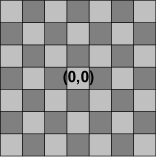
$\mathcal{C}_{2}$

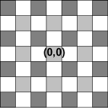
$\mathcal{C}_{1}$

Figure 1: Relation between “coloring” for $\mathcal{C}_{2}$ and $\mathcal{C}_{1}$

Relation between “coloring” for $\mathcal{R}_{2}$ ($\mathcal{C}_{2}$) and $\mathcal{R}_{1}$ ($\mathcal{C}_{1}$) is shown on Fig. 1. For $\mathcal{R}_{2}$ ($\mathcal{C}_{2}$) coloring of cell $(i,j)$ used for illustration properties above is corresponding to value $i+j\mod 2$. Next, all the $\mathcal{C}_{2}$ board is mapped into sublattice of $\mathcal{C}_{1}$ producing new type of coloring with “light” and “dark” cells illustrated on Fig. 1.

Due to such a map $\mathcal{C}_{2}$ corresponds to sublattice $c^{\prime}$ in $\mathcal{C}_{1}$ with coordinates $c_{i+j,i-j}$ Eq. (23). New indexes $(i+j,i-j)$ are both either odd or even.

Let us use for $\mathcal{R}_{1}$ notation already introduced for $\mathcal{R}_{2}$ with $c_{1}$ and $c_{2}$ configurations corresponding to set of cells with nonzero first and second elements in the pair representing a state of second-order CA.

It was shown that for configurations derived from a single cell with unit state such patterns have opposite color. For $\mathcal{C}_{2}$ it corresponds to different diagonal sublattices and in each pattern nonempty cells can not have adjoint sides, but may have common corners. For $\mathcal{C}_{2}$ with new scheme of coloring the corners of cells are also separated.

Let us first prove such expressions as Eq. (11) and Eq. (12). They already were derived above from Eq. (9) and Eq. (10), but direct proof provided below illustrates some useful relations. The equation Eq. (12) may be derived from Eq. (39) and Eq. (41). Let us recollect that for any polynomial $p(x,y)$ over GF(2)

$$p^{2}(x,y)=(\sum c_{i,j}x^{i}y^{j})^{2}=\sum(c_{i,j}x^{i}y^{j})^{2}=\sum(c_{i,j}x^{2i}y^{2j})$$ (44)

and so for representations of two-states pattern via polynomials used earlier the square corresponds to rescaling of the pattern $(i,j)\mapsto(2i,2j)$. The Eq. (39) corresponds to multiplication of $T(x,y)$ on the rescaling pattern. For $\mathcal{C}_{1}$ $T(x,y)$ is described by Eq. (29).

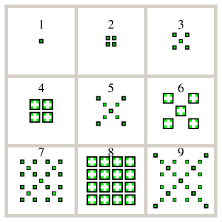
Figure 2: Recursion Eq. (12) for $R_{2}(n)$ in $\mathcal{C}_{1}$

It was already shown, that for $\mathcal{C}_{1}$ any cells with same value are separated, so after the scaling distances between nonzero cells are enough to put four new cells generated by $T(x,y)$ without overlap. Fig. 2 illustrates that for

$$n=1~{}{}_{\times 4}\to n=2~{}{}_{\times 4}\to n=4~{}{}_{\times 4}\to n=8,\quad n=3~{}{}_{\times 4}\to n=6.$$

So, Eq. (39) proves first part of Eq. (12), $R_{2}(2n)=4R_{2}(n)$.

Next, due to Eq. (1) two polynomials $f_{n+1}$, $f_{n}$ in Eq. (41) describes $(c_{1},c_{2})$ on a step $n$ and it was already shown that the pattern are not intersecting for chosen initial conditions. Square of the sum only rescales the union without changing number of nonzero cells. Fig. 2 illustrates that for

$$n=1\cup 2\to n=3,~{}n=2\cup 3\to n=5,~{}n=3\cup 4\to n=7,~{}n=4\cup 5\to n=9.$$

So, Eq. (41) proves second part of Eq. (12), $R_{2}(2n+1)=R_{2}(n+1)+R_{2}(n)$. $\square$

Recursive polynomial equation Eq. (43) can be simply adopted for proof of Eq. (10) for number of cells in $\mathcal{R}_{1}$ and $\mathcal{R}_{2}$ and it is enough to demonstrate both Eq. (8) and Eq. (9).

Let us prove Eq. (10) for number of cells with state 2 in $\mathcal{R}_{1}$ using Eq. (43). The fact, that all cells with state 2 on each step $k$ are contained within a square region represented as direct product of two open intervals $(-k,k)\times(-k,k)$ is also used and proved.

For $k=0,1$ and initial configuration the Eq. (10) holds and estimation for shape of square boundary is also true (for $k=0$ region is empty).

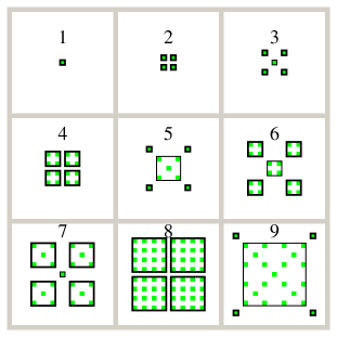
Figure 3: Composition Eq. (10) for $R_{2}(n)$ in $\mathcal{R}_{1}$

Assume that equations hold for all patterns $j\leq 2^{n}$ and consider $j^{\prime}=2^{n}+j$. Due to Eq. (43) and Eq. (24) the polynomial representation is

$$p_{2^{n}+j}=(x^{-2^{n}}y^{-2^{n}}\!+x^{2^{n}}y^{-2^{n}}\!+x^{-2^{n}}y^{2^{n}}\!+x^{2^{n}}y^{2^{n}})\,p_{j}+p_{2^{n}-j}.$$ (45)

The multiplier before $p_{j}$ produces four copies moved in directions $(-2^{n},-2^{n})$, $(-2^{n},+2^{n})$, $(+2^{n},-2^{n})$, $(+2^{n},+2^{n})$ and $p_{2^{n}-j}$ corresponds to pattern in the center, Fig. 3. The five patterns are not overlapped: central one with $R_{2}(2^{n}-j)$ nonempty cells is contained within $(-j^{\prime}+j,j^{\prime}-j)\times(-j^{\prime}+j,j^{\prime}-j)$ and other four others with $R_{2}(j)$ nonempty cells are distributed within a “four-fold” disjointed region described by product

$$\{(-j^{\prime},-j^{\prime}+j)\cup(j^{\prime}-j,j^{\prime})\}\times\{(-j^{\prime},-j^{\prime}+j)\cup(j^{\prime}-j,j^{\prime})\}.$$

Total number of nonempty cells is $4R_{2}(j)+R_{2}(2^{n}-j).$ So the equation for number of cells Eq. (10) holds for $j^{\prime}\leq 2^{n+1}$. The union of the five regions belongs to square $(-j^{\prime},j^{\prime})\times(-j^{\prime},j^{\prime})$. $\square$

Fig. 3 illustrates relations

$$n=1~{}{}_{\times 4}\to n=2~{}{}_{\times 4}\to n=4~{}{}_{\times 4}\to n=8,$$

$$n=1~{}{}_{\times(4+1)}\to n=3,\quad n=2~{}{}_{\times(4+1)}\to n=6,$$

$$n=1_{\times 4}\cup 3\to n=5,\quad n=3_{\times 4}\cup 1\to n=7,\quad n=1_{\times 4}\cup 8\to n=9.$$

The five patterns have a unit gap between them (Fig. 3) and only after consideration of all cells with nonzero values corresponding to union of both “checkerboard sublattices” the final patterns (Fig. 4) belong to square regions described by product of closed intervals $[-k,k]\times[-k,k]$ and recursive equation Eq. (8) corresponds to union of five disjoint regions without gaps, Fig. 4.

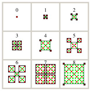
Figure 4: Composition Eq. (8) for $R(n)$ in $\mathcal{R}_{1}$

Fig. 4 illustrates relations

$$n=0_{\times 5}\to n=1,\quad n=0_{\times 4}\cup 1\to n=2,\quad n=0\cup 1_{\times 4}\to n=3,$$

$$n=0_{\times 4}\cup 3\to n=4,\quad n=1_{\times 4}\cup 2\to n=5,\quad n=2_{\times 4}\cup 1\to n=6,$$

$$n=0\cup 3_{\times 4}\to n=7,\quad n=0_{\times 4}\cup 7\to n=8.$$

Let us check recursive equation for pair of polynomials Eq. (31) representing all states of second-order CA and used for calculation of $R(n)$

$$P[C_{2^{k}+j}] = \bigl{(}f_{2^{k}+j+1}(T),f_{2^{k}+j}(T)\bigr{)}$$ (46)

$$= \bigl{(}T^{2^{k}}f_{j+1}(T)+f_{2^{k}-j-1}(T),T^{2^{k}}f_{j}(T)+f_{2^{k}-j}(T)\bigr{)}$$

$$= T^{2^{k}}\bigl{(}f_{j+1}(T),f_{j}(T)\bigr{)}+\bigl{(}f_{2^{k}-j-1}(T),f_{2^{k}-j}(T)\bigr{)}$$

$$= T^{2^{k}}P[C_{j}]+P[{\mathsf{X}}C_{2^{k}-j-1}],$$

where $\mathsf{X}$ operation Eq. (4) swaps values $1\leftrightarrow 2$.

The Eq. (46) illustrates dynamics of pattern growth, Fig. 4. Due to Eq. (3) application of transition rule $F$ to pattern ${\mathsf{X}}C_{i}$ for any index $i>0$ satisfies property

$$F:\mathsf{X}C_{i}\mapsto\mathsf{X}C_{i-1},$$ (47)

so, application of $F$ to Eq. (46) corresponds to increase of four patterns $C_{j}$ and decrease of central region ${\mathsf{X}}C_{2^{k}-j-1}$ until $2^{k}-j-1>0$. For $j=2^{k}-1$ four outer configurations reach maximal size and may not grow more, so on next step they are joined into single central configurations $XC_{2^{k+1}-1}$ and four cells $C_{0}$ appear near corners as centers for future growth.

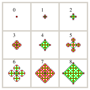
Figure 5: Composition Eq. (8) for $R(n)$ in $\mathcal{R}_{2}$

Proofs of Eqs. (8–12) for $\mathcal{R}_{2}$ directly follow from consideration of $\mathcal{R}_{1}$, because (similarly with relation between $\mathcal{C}_{1}$ and $\mathcal{C}_{2}$ discussed earlier) $\mathcal{R}_{2}$ is equivalent with $\mathcal{R}_{1}$ acting on a diagonal sublattice.

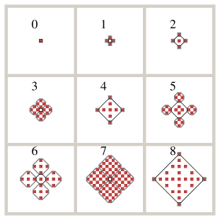
Figure 6: $\mathcal{R}_{2}$, $\mathcal{R}_{3}$, $\mathcal{R}_{3}^{\prime}$ — cells with value 1

In such representation patterns for $\mathcal{R}_{2}$ may look more closely packed Fig. 5, but it does not change recursive equations due to above mentioned equivalence. Let us now consider $\mathcal{R}_{3}$ and $\mathcal{R}_{3}^{\prime}$.

Local rule for both $\mathcal{R}_{2}$ and $\mathcal{R}_{3}$ uses only four closest cells with common sides in so-called von Neumann neighborhood. Due to Eq. (1) it is enough to consider actions of local rules for $\mathcal{C}_{2}$ and $\mathcal{C}_{3}$ on the first element of pair to describe differences between rules. If the rules act in the same way for any configuration under consideration, then actions of $\mathcal{R}_{2}$ and $\mathcal{R}_{3}$ for patterns derived from $\Delta_{0,0}$ are also the same.

Comparison of definition $\mathcal{C}_{2}$ and $\mathcal{C}_{3}$ shows that local rules differ only for three nonempty cells in von Neumann neighborhood. On Fig. 6 for simplicity are shown only cells with nonzero first components in the pair for configurations used earlier, Fig. 5.

All such pattern have 0,1,2,4 nonempty cells in von Neumann neighborhood and so $\mathcal{R}_{2}$ and $\mathcal{R}_{3}$ act in the same way for such pattern. Let us proof the property by induction. Any new configuration is composition of five previous patterns and it is enough to consider new configurations near contiguities of they boundaries.

Due to consideration below for $n\neq 2^{k}-1$ there are four contacts of central pattern with outer configurations. Four cells with two neighbors corresponds them. The cases $n=2^{k}-1$ correspond to contacts of four outer patterns and due to symmetry number of neighbors there are always even. In fact, it may be simply shown that all such configuration (of cells with state 1) are simple diamond-like checkerboard patterns with $2^{k}\times 2^{k}=4^{k}$ cells, Fig. 6.

Let us now consider $\mathcal{R}^{\prime}_{3}$. The only difference between $\mathcal{C}^{\prime}_{3}$ and $\mathcal{C}_{3}$ is additional requirement about cells with common corners. The limitation always holds due to “coloring” properties already discussed earlier on page 5. Indeed, each new generation of cells with state 1 for $\mathcal{R}_{2}$ may appear only on checkerboard sublattice with opposite colors, i.e. all cells with common corner for an empty cell going to be switched into the state 1 are empty. So, evolution of $\mathcal{R}^{\prime}_{3}$ starting with configuration $\Delta_{0,0}$ is also the same as for $\mathcal{R}_{3}$ and $\mathcal{R}_{2}$. $\square$

References

[1]T. Toffoli and N. Margolus, “Invertible cellular automata: a review,”
Physica D 45, 229–253 (1990).
[2]S. Wolfram, Cellular automata and complexity: Collected papers,
(Addison-Wesley, Reading MA 1994).
[3] L. Le Bruyn and M. Van den Bergh, “Algebraic properties of
linear cellular automata,” Lin. Alg. Appl. 157,
217–234 (1991).
[4] S. Wolfram, “Statistical mechanics of cellular automata,”
Rev. Mod. Phys. 55, 601–644 (1983); reprinted in [2], 3–70.
[5] O. Martin, A. M. Odlyzko, and S. Wolfram, “Algebraic properties
of cellular automata,” Comm. Math. Phys. 93, 219–258 (1984);
reprinted in [2], 71–113.
[6] B. Chopard and M. Droz, Cellular automata modeling of physical
systems, (Cambridge University Press, Cambridge 1998).
[7] T. Koshy, Fibonacci and Lucas numbers with applications,
(John Wiley & Sons, New York, 2001).