labelkeycmyk.4,.2,0,0

Avalanche shape and exponents beyond mean-field theory

Abstract

Elastic systems, such as magnetic domain walls, density waves, contact lines, and cracks, are all pinned by substrate disorder. When driven, they move via successive jumps called avalanches, with power law distributions of size, duration and velocity. Their exponents, and the shape of an avalanche, defined as its mean velocity as function of time, have recently been studied. They are known approximatively from experiments and simulations, and were predicted from mean-field models, such as the Brownian force model (BFM), where each point of the elastic interface sees a force field which itself is a random walk. As we showed in EPL 97 (2012) 46004, the BFM is the starting point for an $\varepsilon=d_{\rm c}-d$ expansion around the upper critical dimension, with $d_{\rm c}=4$ for short-ranged elasticity, and $d_{\rm c}=2$ for long-ranged elasticity. Here we calculate analytically the ${\cal O}(\varepsilon)$, i.e. 1-loop, correction to the avalanche shape at fixed duration $T$, for both types of elasticity. The exact expression is well approximated by $\left<\dot{u}(t=xT)\right>_{T}\simeq[Tx(1-x)]^{\gamma-1}\exp\left({\cal A}\left[\frac{1}{2}-x\right]\right)$, $0<x<1$. The asymmetry ${\cal A}\approx-0.336(1-d/d_{\rm c})$ is negative for $d$ close to $d_{\rm c}$, skewing the avalanche towards its end, as observed in numerical simulations in $d=2$ and $3$. The exponent $\gamma=(d+\zeta)/z$ is given by the two independent exponents at depinning, the roughness $\zeta$ and the dynamical exponent $z$. We propose a general procedure to predict other avalanche exponents in terms of $\zeta$ and $z$. We finally introduce and calculate the shape at fixed avalanche size, not yet measured in experiments or simulations.

Phase transitions and critical phenomena

Introduction:

An elastic interface driven through a disordered medium is an efficient mesoscopic model for a number of different physical systems, such as the motion of domain walls in soft magnets [1], fluid contact lines on a rough surface [2], or strike-slip faults in geophysics; see [3] for a review. Their response to external driving is not smooth, but exhibits collective jumps called avalanches, extending over a broad range of space and time scales. They can be detected e.g. as pulses of Barkhausen noise in magnets [4, 5], slip instabilities leading to earthquakes on geological faults, or in fracture experiments [6]. While the microscopic details of the dynamics are specific to each system, an important question is whether the large-scale features are universal. A prominent example are the exponents of the power-law distribution function (PDF) of avalanche sizes $P(S)\sim S^{-\tau}$ (for earthquakes, the Gutenberg-Richter law) and durations. Beyond scaling exponents, the question of whether the shape of an avalanche is universal is of great current interest in theory and experiments [7, 8]. Understanding how universality arises, which quantities are universal, and how to make quantitative predictions beyond phenomenological models are some of the main challenges in the field.

Historically, the elastic-interface model allowed for analytical progress thanks to a powerful method, the Functional Renormalization group (FRG). It was first developed to calculate the static (equilibrium) deformations of an interface pinned by a random potential (e.g. the roughness exponent), or the critical dynamics at and beyond the depinning transition, applying an external force $f\geq f_{\rm c}$ [9, 10, 11, 12]. These results were obtained in an expansion in the internal space dimension $d$ of the interface around the upper critical dimension $d_{\rm c}$, equivalent to a loop expansion. Despite these successes, the study of avalanches in elastic systems has remained centered on toy models [3, 13, 14], scaling arguments, and numerics [15, 16, 17, 11, 18]. Other important models used to describe avalanches are the random-field Ising model [19], mean-field spin glasses [20], and discrete automata alias sandpile models, with some analytical results [21, 22, 23]. However, exact results on the avalanche statistics are notably hard to obtain. Recently, we have extended the FRG-based field theory to calculate the avalanche-size distribution [24, 25] in dimension $d<d_{\rm c}$, with excellent agreement to numerics [24, 26]. We then extended the theory to the dynamics and obtained the velocity distribution within an avalanche [27].

In this Letter, we use this theory to propose several novel scaling relations for avalanche exponents, and calculate the shape of an avalanche, both at fixed duration and at fixed size. Since the calculations are very technical, we only sketch the main ingredients of the method and present the key results; the details are given in a separate publication [28]. For an early presentation of this work see [29].

Avalanche densities and dynamical action:

Consider the equation of motion for a driven elastic interface in presence of quenched disorder,

$$\eta\partial_{t}u_{xt}=\nabla_{x}^{2}u_{xt}-m^{2}u_{xt}+f_{t}+F(u_{xt},x)\ .$$ (1)

We denote by subscript the dependence on space and time. Choosing $f_{t}=m^{2}w_{t}$ the interface is bound by a parabolic well of curvature $m^{2}$ (the mass) to an external degree of freedom $w_{t}$. The pinning force $F(u,x)$ is chosen Gaussian with (microscopic) correlator (overlines denote disorder averages)

$$\overline{F(u,x)F(u^{\prime},x^{\prime})}=\delta^{d}(x-x^{\prime})\Delta_{0}(u-u^{\prime}).$$ (2)

Intermittent avalanche motion occurs for slow driving, either at small constant velocity $w_{t}=vt$, or upon a small force step, i.e. a kick $\dot{w}_{t}=w\delta(t)$. Avalanche-size and duration distributions, as well as the shape, can be retrieved from the generating function, i.e. the disorder average of

$$G[\lambda,f]:=\overline{\mathrm{e}^{\int_{x,t}\lambda_{xt}\dot{u}_{xt}}}^{f},$$ (3)

in presence of a source $\lambda_{xt}$ and a driving force $f_{t}=m^{2}w_{t}$. For instance, the PDF of the size of an avalanche, $S:=\int_{x,t>0}\dot{u}_{xt}$, following a kick $f_{t}=m^{2}w\delta(t)$, is the inverse Laplace transform, $P_{w}(S)=\mbox{LT}^{-1}_{-\lambda\to S}G[\lambda,f]$ for a uniform source $\lambda_{xt}=\lambda$. From it one defines a size density (per unit displacement $w$), $\rho(S):=\partial_{w}P_{w}(S)|_{w=0^{+}}$, which equals the size density defined from stationary motion at fixed $v=0^{+}$. Similarly one defines the density for the avalanche duration $T$. All these densities, for sizes $S\ll S_{m}$ and times $T\ll\tau_{m}$, obey power laws with exponents

$$\rho(S)\sim S^{-\tau}\quad,\quad\rho(T)\sim T^{-\alpha}\ ,$$ (4)

where $S_{m}$ and $\tau_{m}$ are set by the mass (and $\eta$ for $\tau_{m}$) and are used as convenient units below.

	$\rho(S)$	$\rho(S_{\phi})$	$\rho(T)$	$\rho(\dot{u})$	$\rho(\dot{u}_{\phi})$
	$S^{-\tau}$	$S_{\phi}^{-\tau_{\phi}}$	$T^{-\alpha}$	$\dot{u}^{-\sf a}$	$\dot{u}_{\phi}^{{-\sf a}_{\phi}}$
short-ranged elasticity (SR)	$\tau=2-\frac{2}{d+\zeta}$	$\tau_{\phi}=2-\frac{2}{d_{\phi}+\zeta}$	$\alpha=1+\frac{d-2+\zeta}{z}$	${\sf a}=2-\frac{2}{d+\zeta-z}$	${\sf a}_{\phi}=2-\frac{2}{d_{\phi}+\zeta-z}$
long-ranged elasticity (LR)	$\tau=2-\frac{1}{d+\zeta}$	$\tau_{\phi}=2-\frac{1}{d_{\phi}+\zeta}$	$\alpha=1+\frac{d-1+\zeta}{z}$	${\sf a}=2-\frac{1}{d+\zeta-z}$	${\sf a}_{\phi}=2-\frac{1}{d_{\phi}+\zeta-z}$

Table 1: Scaling relations

To calculate $G[\lambda,f]$, one takes a time-derivative of Eq. (1),

$$\eta\partial_{t}\dot{u}_{xt}=\nabla_{x}^{2}\dot{u}_{xt}+f_{t}-m^{2}\dot{u}_{xt}+\partial_{t}F(u_{xt},x),$$ (5)

and constructs the dynamical field theory by multiplying this equation with a response-field $\tilde{u}_{xt}$. Averaging over disorder leads to the path-integral representation

$$G[\lambda,f]=\int{\cal D}[\dot{u}]{\cal D}[\tilde{u}]\mathrm{e}^{-{\cal S}_{\lambda,f}[u,\tilde{u}]}\ .$$ (6)

The dynamical action reads

$${\cal S}_{\lambda,f}[u,\tilde{u}]={\cal S}_{0}[u,\tilde{u}]+{\cal S}_{\rm dis}[u,\tilde{u}]+\int_{xt}\lambda_{xt}\dot{u}_{xt}$$ (7)

$$\!\!\!{\cal S}_{0}[u,\tilde{u}]=\int_{xt}\tilde{u}_{xt}\left[\eta\partial_{t}\dot{u}_{xt}-\nabla^{2}\dot{u}_{xt}+m^{2}\dot{u}_{xt}-f_{t}\right]$$ (8)

$$\!\!\!{\cal S}_{\rm dis}[u,\tilde{u}]=-\frac{1}{2}\int_{x,t,t^{\prime}}\tilde{u}_{xt}\tilde{u}_{x,t^{\prime}}\partial_{t}\partial_{t^{\prime}}\Delta_{0}(u_{xt}-u_{xt^{\prime}})\,.$$ (9)

Upon coarse-graining, the action becomes the effective action ${\cal S}_{\rm dis}\to{\cal S}^{\rm eff}_{\rm dis}$, with a renormalized disorder correlator $\Delta(u)$, which takes a non-analytic form with a linear cusp at $u=0$,

$$\Delta_{0}(u)\to\Delta(u)=\Delta(0)-\sigma|u|-\frac{g}{2}u^{2}+...$$ (10)

with $\sigma=-\Delta^{\prime}(0^{+})$, and $g=-\Delta^{\prime\prime}(0^{+})$. Hence one can rewrite [27]

$${\cal S}^{\rm eff}_{\rm dis}[u,\tilde{u}] = -\sigma\int_{x,t}\tilde{u}_{xt}^{2}\dot{u}_{xt}$$ (11)

$$-\frac{g}{2}\int_{x,t,t^{\prime}}\tilde{u}_{xt}\dot{u}_{xt}\,\tilde{u}_{xt^{\prime}}\dot{u}_{xt^{\prime}}+...$$

Note that while the disorder interaction is in general non-local in time, the first term, proportional to $\sigma$, is local, since $\frac{\mathrm{d}^{2}}{\mathrm{d}u^{2}}|u|=2\delta(u)$; a simplifying feature to be exploited below.

Mean-field theory: the Brownian force model.

Further suppose that the microscopic force correlator (10) only contains the term $-\sigma|u|$, realized if for each $x$ the forces $F(u,x)$ are chosen as Brownian motions in $u$ uncorrelated in $x$. One then shows that $\Delta(u)$ does not change under renormalization [27, 31], i.e. the renormalized model is also given by Eq. (10) with $g=0$. This is the Brownian force model (BFM) introduced in [27]. It has a very simple local action, given by Eq. (11) with only the first term $\sim\sigma$. Since the velocity $\dot{u}_{xt}$ appears linearly in Eqs. (7), (8) and (11), the field theory is exactly solvable [27, 31],

$$G[\lambda,f]=e^{\int_{x,t}f_{t}\tilde{u}_{xt}^{\lambda}}\ .$$ (12)

Here $\tilde{u}_{xt}^{\lambda}$ is the solution of the (exact) saddle-point or instanton equation $\frac{\delta{\cal S}_{\lambda,f}}{\delta\dot{u}_{xt}}=0$, namely

$$\eta\partial_{t}\tilde{u}_{xt}^{\lambda}+(\nabla^{2}-m^{2})\tilde{u}_{xt}^{\lambda}+\sigma(\tilde{u}_{xt}^{\lambda})^{2}=-\lambda_{xt}\ .$$ (13)

The superscript $\lambda$ indicates that $\tilde{u}_{xt}^{\lambda}$ depends on $\lambda_{xt}$. This allows to calculate many observables exactly [27, 31]. To simplify the calculations, one can express all observables

	$d$	$\zeta$	$z$	$\tau$	$\tau_{\phi}$	$\alpha$	${\sf a}$	${\sf a}_{\phi}$	$\gamma$
	$1$	$1.25$	$1.433$	$1.11$	$0.4$	$1.17$	$-0.45$	$12.9$	$1.57$
SR	$2$	$0.75$	$1.56$	$1.27$	$-0.67$	$1.48$	$0.32$	$4.47$	$1.76$
	$3$	$0.35$	$1.75$	$1.40$	$-3.71$	$1.77$	$0.75$	$3.43$	$1.91$
LR	$1$	$0.39$	$0.77$	$1.28$	$-0.56$	$1.51$	$0.39$	$4.63$	$1.81$

Table 2: Critical exponents obtained via the scaling relations using standard values for $\zeta,z$ [33]. For the local avalanche exponents we consider a point, $d_{\phi}=0$.

in units of $S_{m}=\sigma/m^{4}$ and $\tau_{m}=\eta/m^{2}$, equivalent to setting $m^{2}=\sigma=\eta=1$. For a uniform source $\lambda_{xt}=\lambda$ one finds $\tilde{u}_{xt}^{\lambda}=\frac{1}{2}\left(1-\sqrt{1-4\lambda}\right)$ which leads for a kick $f_{t}=m^{2}w\delta(t)$ to $P_{w}(S)=\frac{wL^{d}}{2\sqrt{\pi}S^{3/2}}e^{-(S-m^{2}w)^{2}/4S}$ and, in the limit of $w\to 0$, to the famous [13, 14] mean-field size density $\rho(S)=\frac{L^{d}}{2\sqrt{\pi}S^{\tau^{\rm MF}}}\mathrm{e}^{-S/4}$ with $\tau^{\rm MF}=\frac{3}{2}$. Indeed, all observables containing only the center-of-mass are equivalent [27] to those of the phenomenological ABBM model [13, 14], which is nothing but the BFM in $d=0$. However, the BFM can go further and allows to obtain the dependence on system size $L$, kick amplitude $w$, as well as local observables, such as the motion of a small piece of the interface, or the response to a local kick. Splitting $x=(x_{\parallel},x_{\perp})$ with $x_{\parallel}\in\mathbb{R}^{d_{\phi}},x_{\perp}\in\mathbb{R}^{d-d_{\phi}}$, we focus on the submanifold $\phi$ of dimension $d_{\phi}$ given by $x=(x_{\parallel},0)$. The local size of an avalanche on $\phi$ is

$$S_{\phi}=\int\mathrm{d}t\int\mathrm{d}^{d_{\phi}}x_{\parallel}\,\dot{u}_{(x_{\parallel},x_{\perp}=0),t}\ .$$ (14)

It is expressed in units of $S_{m}^{\phi}=S_{m}m^{d-d_{\phi}}$, see below. Explicit solution of (13) for the corresponding source $\lambda_{xt}=\lambda\delta^{d-d_{\phi}}(x_{\perp})$ is possible for $d_{\phi}=d-1$, leading to $\rho(S_{\phi})=\frac{2L^{d_{\phi}}}{\pi S_{\phi}}{\rm K}_{1/3}(2S_{\phi}/\sqrt{3})\sim S_{\phi}^{-\tau_{\phi}^{\rm MF}}$ in terms of a Bessel function [25] , with (in that case) $\tau_{\phi}^{\rm MF}=\frac{4}{3}$.

Dynamical observables can be obtained from the solution $\tilde{u}^{\lambda}_{xt}=\frac{\lambda\theta(T-t)}{\lambda+(1-\lambda)\mathrm{e}^{T-t}}$ of (13) with the source $\lambda_{xt}=\lambda\delta(T-t)$ [27, 31]. Applying a kick at time $t=0$ and taking $\lambda\to-\infty$ selects $\dot{u}_{x,T}=0$, i.e. the avalanches of duration smaller than $T$. From $\tilde{u}^{\lambda}_{x,0}$ and using Eqs. (3) and (12) one obtains the PDF of durations as $P_{w}(T)=\frac{wL^{d}}{(2\sinh T/2)^{2}}e^{-wL^{d}/(e^{T}-1)}$. It converges to a Gumbel distribution for $wL^{d}\gg 1$ (longest duration among many independent avalanches), while for $wL^{d}\ll 1$ it leads to the known mean-field duration-density [14] with exponent $\alpha^{\rm MF}=2$. Calculating instead $\int_{t}\tilde{u}^{\lambda}_{xt}=-\ln(1-\lambda)$ for a constant driving $\dot{w}_{t}=v$, one obtains the stationary PDF of the total instantaneous velocity,

$$\dot{\sf u}_{t}:=\int_{x}\dot{u}_{xt}\;,$$ (15)

as $P_{v}(\dot{\sf u})=\dot{\sf u}^{-1+vL^{d}}e^{-\dot{\sf u}}/\Gamma(vL^{d})$, in units of $v_{m}=S_{m}/\tau_{m}$. For $vL^{d}\ll 1$ it yields the density $\rho(\dot{\sf u})=\frac{L^{d}}{\dot{\sf u}}\mathrm{e}^{-\dot{\sf u}}$, in agreement with the $d=0$ velocity distribution [13, 14].

Figure 1: Diagrammatic representation of the 1-loop corrections to the shape at fixed duration (The shape at fixed duration:) (similarly for (34)). Solid lines are response functions, doubled for dressed ones, defined in [27]; they account for the non-vanishing expectation of $\tilde{u}_{xt}$ in Eq. (13). Dashed lines are $g$-vertices, the other vertices are $\sigma$. Internal times and the loop momentum are integrated over.

Field theory beyond the Brownian force model:

It was shown in [27] that the BFM is the mean-field limit of the field theory defined by Eqs. (6), (7), i.e. it gives the joint multi-space-time-point velocity PDF in a single avalanche for $d\geq d_{\rm c}$ . Moreover, including the term $\sim g$ in Eq. (10) is sufficient to obtain the complete 1-loop corrections, i.e. to calculate these distributions to first order in an expansion in $\varepsilon=d_{\rm c}-d$, with $g={\cal O}(\varepsilon)$ at the fixed point. The velocity density was obtained to one loop [27], with a non-trivial tail for $\dot{\sf u}\gg 1$, and a power-law singularity

$$\rho(\dot{\sf u})\simeq_{\dot{\sf u}\ll 1}\frac{CL^{d}}{\dot{\sf u}^{\sf a}},\quad{\sf a}=1-\frac{2}{9}\varepsilon+O(\varepsilon^{2})\,,$$ (16)

with $C=1-\frac{\varepsilon}{9}(4\gamma_{\rm E}+\frac{1}{2}-2\ln 2)$.

Exponent relations:

At the level of the field theory of depinning, i.e. Eq. (7) to two loops, and for avalanches Eq. (11) to one loop, until now we have found only two independent renormalizations, one for the disorder $\sigma\to\sigma_{m}$, and one for the friction $\eta\to\eta_{m}$, leading to two independent scales in any dimension $d$:

$$S_{m}=\sigma_{m}/m^{4}\sim m^{-(d+\zeta)}\ ,\quad\tau_{m}=\eta_{m}/m^{2}\sim m^{-z}\ .$$ (17)

This suggests that avalanche exponents, such as $\tau$, $\alpha$ and ${\sf a}$ are not independent, but instead related to the roughness $\zeta$ and dynamical exponent $z$. Starting with the Narayan Fisher (NF) conjecture [11] for $\tau$, this has been a recurrent question in the field [18], and, for the velocity exponent ${\sf a}$, an outstanding one.

We now reexamine and extend the NF conjecture using dimensional and field theoretic arguments. Restoring units (i.e. all factors of $m$), the size density (per unit $w$) takes the form $\rho(S)=L^{d}S_{m}^{-2}(S_{m}/S)^{-\tau}f(S/S_{m})$ with $f(0)$ a finite constant. The NF conjecture is equivalent to stating that the size density per unit force, $\rho_{f}(S)=m^{-2}\rho(S)$, has a finite (infrared-cutoff independent) limit $m\to 0$, i.e.

$$\rho_{f}(S)\sim L^{d}{S^{-\tau}}f(S/S_{m})\ ,$$ (18)

up to a constant prefactor. This implies $S_{m}^{2-\tau}\sim m^{2}$, i.e.

$$\tau=2-\frac{2}{d+\zeta}\ .$$ (19)

In the field theory, one can use the exact relation

$$\int\mathrm{d}S(\mathrm{e}^{\lambda S}-1)\rho_{f}(S)=L^{d}\langle\tilde{u}_{x,t=0}\rangle_{\lambda}\ .$$ (20)

Upon the same assumption (18) the result (19) can equivalently be obtained from Eq. (20): In the action (7) the term $\int_{xt}\tilde{u}_{xt}m^{2}\dot{u}_{xt}$ is protected by the statistical tilt symmetry, hence the response field has dimension $\tilde{u}_{xt}\sim m^{d-2+\zeta}$. Matching the l.h.s. at $-\lambda=1/S_{m}$ yields $(-\lambda)^{\tau-1}\sim S_{m}^{1-\tau}\sim m^{d-2+\zeta}$ recovering Eq. (19). The field theory confirms that the quantity which must have a $m\to 0$ limit is $\rho_{f}(S)$, and not $\rho(S)$, in order that (19) holds.

Consider now the distribution of the total velocity $\dot{\sf u}$ defined in Eq. (15), and define the density per unit force change $\dot{f}=m^{2}v$,

$$\rho_{f}(\dot{\sf u})=\partial_{\dot{f}}P_{v}(\dot{\sf u})|_{\dot{f}=0^{+}}\ .$$ (21)

It diverges as $m^{2}\rho_{f}(\dot{\sf u})\sim\frac{L^{d}}{(v_{m})^{2}}(v_{m}/\dot{\sf u})^{\sf a}$ by dimensional analysis, where $v_{m}=S_{m}/\tau_{m}$. The existence of a massless limit for $\rho_{f}(\dot{\sf u})$ implies $(v_{m})^{{\sf a}-2}\sim m^{2}$; hence, from Eq. (17) we obtain the new relation

$${\sf a}=2-\frac{2}{d+\zeta-z}\ .$$ (22)

In the field theory, this identity can be derived from

$$\int\mathrm{d}\dot{\sf u}(e^{\lambda\dot{\sf u}}-1)\rho_{f}(\dot{\sf u})=L^{d}\int_{t}\langle\tilde{u}_{xt}\rangle_{\lambda}$$ (23)

with the source $\lambda_{xt}=\lambda\delta(t)$ and an additional integral over the time where the avalanche was triggered. Assuming that a massless limit exists for $\rho_{f}(\dot{\sf u})\sim\dot{\sf u}^{-{\sf a}}$, we can match the l.h.s of Eq. (23) at $\dot{\sf u}\sim v_{m}$, as $(-\lambda)^{{\sf a}-1}\sim v_{m}^{1-{\sf a}}$ and identify its mass dimension as $\sim m^{d-2+\zeta-z}$ from the r.h.s., leading again to Eq. (22).

This can be generalized to local avalanche observables. Assuming again a massless limit for densities per unit force one finds $(S^{\phi}_{m})^{\tau_{\phi}-2}\sim m^{2}$ and the local avalanche-size density

$$\rho(S_{\phi})\sim_{S_{\phi}\ll S^{\phi}_{m}}{S_{\phi}^{-\tau_{\phi}}}\ ,\qquad\tau_{\phi}=2-\frac{2}{d_{\phi}+\zeta}\ .$$ (24)

For the local velocity density one finds $(v^{\phi}_{m})^{{\sf a}_{\phi}-2}\sim m^{2}$ where $v^{\phi}_{m}=S^{\phi}_{m}/\tau_{m}$ is the natural unit, and consequently

$$\rho(\dot{\sf u}_{\phi})\sim_{\dot{\sf u}_{\phi}\ll v^{\phi}_{m}}\dot{\sf u}_{\phi}^{{-\sf a}_{\phi}}\ ,\qquad{\sf a}_{\phi}=2-\frac{2}{d_{\phi}+\zeta-z}\ .$$ (25)

Similar arguments for the duration distribution lead to

$$\rho(T)\sim_{T\ll\tau_{m}}{T^{-\alpha}}\ ,\qquad\alpha=1+\frac{d-2+\zeta}{z}\ ,$$ (26)

recovering the result of [18] obtained by simple scaling from (17) and the variable change $\mathrm{d}S\,\rho(S)=\mathrm{d}T\,\rho(T)$. The mean avalanche size at fixed duration is likewise given by

$$\left<S\right>_{T}\sim_{T\ll\tau_{m}}T^{\gamma}\ ,\qquad\gamma=\frac{d+\zeta}{z}\ .$$ (27)

For LR-elasticity $q^{2}\to|q|$ (in Fourier) the predictions change as indicated on table 1, where all results are summarized. (The formula for $\gamma$ remains the same).

In summary these scaling relations should hold, provided only two independent renormalizations are sufficient to render the field theory of depinning finite. The fact that $\dot{f}_{xt}$ and $\lambda_{xt}$ are linear perturbations of the depinning action suggests that they cannot induce other renormalizations. Numerical values predicted by these conjectures are indicated on table 2; it is important to check them in numerics and experiments.

The shape at fixed duration:

The shape of an avalanche conditioned on its duration $T$ is obtained from our field theory in an expansion in $\varepsilon=d_{\rm c}-d$. The calculation is involved, and we only sketch its diagrammatic representation in Fig. 1. The general result is lengthy, hence we only display its universal limit for short duration $T\ll\tau_{m}$,

$$\left<\dot{\sf u}\left(t=xT\right)\right>_{T} = 2{\cal N}\Big{[}Tx(1-x)\Big{]}^{\gamma-1}$$

$$\times\exp\bigg{(}-\frac{16\varepsilon}{9d_{\rm c}}\bigg{[}\text{Li}_{2}(1-x)-\text{Li}_{2}\Big{(}\frac{1-x}{2}\Big{)}$$

$$~{}~{}~{}~{}~{}~{}+\frac{x\log(2x)}{x-1}+\frac{(x+1)\log(x+1)}{2(1-x)}\bigg{]}\bigg{)},$$

with $d_{\rm c}=4$ for SR and $d_{\rm c}=2$ for LR elasticity. The scaling $\sim T^{\gamma-1}$ is expected from the sum rule $\int_{0}^{T}\mathrm{d}t\,\left<\dot{\sf u}(t)\right>_{T}=\left<S\right>_{T}\sim T^{\gamma}$ and our calculated value $\gamma=2-\frac{4}{9d_{\rm c}}\varepsilon$ is consistent to ${\cal O}(\varepsilon)$ with Eq. (27) . The exponential factor in (The shape at fixed duration:) is regular at $x=0$ and $x=1$. The singular part of the shape, $[x(1-x)]^{\gamma-1}$, is thus symmetric, as anticipated on phenomenological grounds [8], and derived here from first principles. We chose to display Eq. (The shape at fixed duration:) in an exponentiated form so that the amplitudes, ${\cal N}_{{\rm SR}}=e^{-\frac{\varepsilon}{9}[\gamma_{\rm E}-1-2(\ln 2)^{2}-\frac{\pi^{2}}{3}]}$, ${\cal N}_{{\rm LR}}=e^{-\frac{2\varepsilon}{9}[\gamma_{\rm E}-2-2(\ln 2)^{2}-\frac{\pi^{2}}{3}]}$ cancel if one plots the normalized shape

Figure 2: (Universal) normalized shape of an avalanche (of short duration $T\ll\tau_{m}$), for an interface ($d=2$) with SR elasticity. Plotted is the total velocity $\dot{\sf u}(t)$ at time $t=xT$ from Eq. (The shape at fixed duration:), normalized to unit maximum (black thick solid line), compared to: (i) the MF shape $\sim x(1-x)$ (blue, dashed, thin line); (ii) a symmetric scaling-ansatz $\dot{\sf u}\sim[Tx(1-x)]^{1-\frac{\varepsilon}{9}}$ (orange, dot-dashed, thick); (iii) the approximation (29) (green dots), close to the exact result. Inset: ibid. with the MF shape subtracted.

as in Fig. 2. The result (The shape at fixed duration:) is exact${}^{\ref{footnote1}}$ up to terms of order ${\cal O}(\varepsilon^{2})$. Note that, at variance with mean field ($\varepsilon=0$), the full shape is not symmetric under $x\to 1-x$. In fact, the complicated factor in the exponential in (The shape at fixed duration:) turns out to be almost linear, hence a good approximation (ignoring constant prefactors) is

$$\left<\dot{\sf u}\left(t=xT\right)\right>_{T}\sim\Big{[}Tx(1-x)\Big{]}^{\gamma-1}\exp\Big{(}{\cal A}_{d}(\textstyle\frac{1}{2}-x)\Big{)}.$$ (29)

The asymmetry ${\cal A}_{d}$ is defined, e.g. as the slope at $x=\frac{1}{2}$ of the exponential in Eq. (The shape at fixed duration:). Close to $d=d_{\rm c}$ we obtain

$${\cal A}_{d}\approx\textstyle-0.336\left(1-\frac{d}{d_{\rm c}}\right)\ .$$ (30)

An extrapolation of Eq. (The shape at fixed duration:) to $d=2$ for SR elasticity, and $d=1$ for LR elasticity, is plotted in Fig. 2.

Hence we find a negative asymmetry near the upper critical dimension. This is consistent with numerical simulations for SR elasticity in dimensions $d=2,3$, which suggest that avalanches are skewed towards the end, i.e. with Eq. (29) for ${\cal A}_{d=2}\approx-0.065\pm 0.01$ [34]. On the other hand, numerical results in $d=1$ for both SR and LR elasticity suggest skewing towards the beginning [8] with positive asymmetries ${\cal A}_{d=1}\approx 0.08\pm 0.02$ (SR) and ${\cal A}_{d=1}\approx 0.02\pm 0.02$ (LR). To check whether this sign change could be accounted for at 1-loop order, we performed a fixed-$d$, weak-disorder expansion; it does not seem to predict this effect [28]. Hence this sign change, if confirmed, would be a higher-loop effect. Note that the approximate time-reversal symmetry is hard to explain intuitively since “active” regions within an avalanche split over time and become disjoint in space (see e.g. Fig. 1 in [8]). Nevertheless, the ensemble-averaged velocity is almost time-reversal symmetric. The small asymmetries thus result from a delicate balance of several $d$-dependent effects. It would be important to thoroughly test our predictions in $d=2,3$.

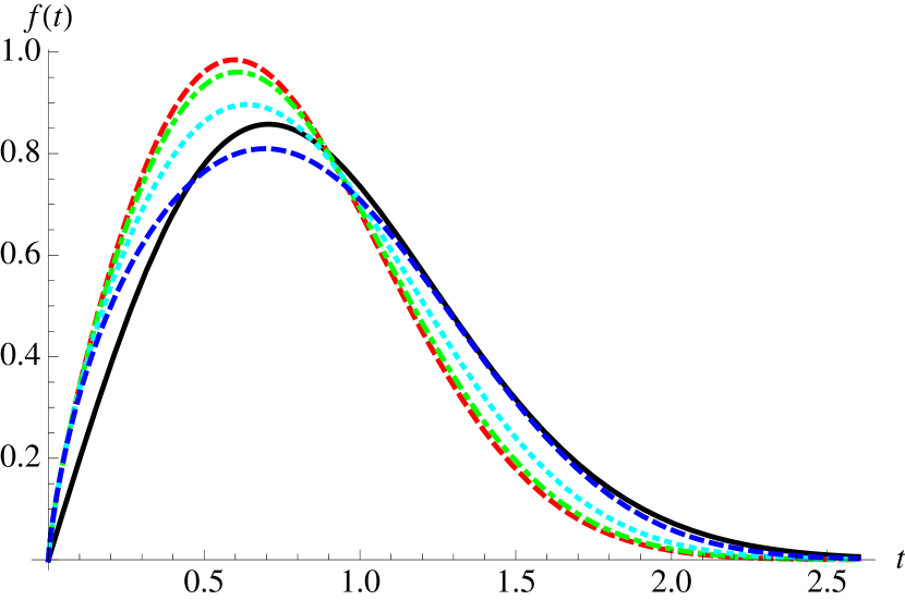
Figure 3: The shape at fixed size, as given by Eq. (37). Mean field (black solid line). The remaining curves are for $\varepsilon=2$: small $S/S_{m}=0^{+}$ limit (red dashed) and $S/S_{m}=1$, $10$, $30$ (green dot-dashed, cyan dotted, and blue dashed).

The shape at fixed size:

We propose to measure a new observable, depending only minimally on the criterion to define the end of an avalanche. It is the mean velocity as a function of time, given that the avalanche size is $S$. Scaling suggests that

$$\langle\dot{\sf u}(t)\rangle_{S}=\frac{S}{\tau_{m}}\Big{(}\frac{S}{S_{m}}\Big{)}^{\!-\frac{1}{\gamma}}f\bigg{(}\frac{t}{\tau_{m}}\Big{(}\frac{S_{m}}{S}\Big{)}^{\!\frac{1}{\gamma}}\bigg{)}$$ (31)

with $\int_{0}^{\infty}\mathrm{d}t\,f(t)=1$, where $f(t)$ may depend on $S/S_{m}$. In mean field, the scaling function $f(t)$ is independent of $S/S_{m}$ [35], and reads

$$f_{0}(t)=2te^{-t^{2}}\quad,\quad\gamma=2\ .$$ (32)

To one loop, i.e. ${\cal O}(\varepsilon)$, for SR elasticity, we obtain

$$f(t)=f_{0}(t)-\frac{\varepsilon}{9}\delta f(t)\quad,\quad\gamma=2-\frac{\varepsilon}{9}\ ,$$ (33)

consistent with (27). Expressions for any $S/S_{m}$ are lengthy and we display only the universal small-avalanche limit:

$$\delta f(t) = \frac{f_{0}(t)}{4}\bigg{[}\pi\left(2t^{2}+1\right)\text{erfi}(t)+2\gamma_{\rm E}\left(1-t^{2}\right)-4$$ (34)

$$~{}~{}~{}~{}~{}~{}~{}~{}-2t^{2}\left(2t^{2}+1\right)\,_{2}F_{2}\left(1,1;\frac{3}{2},2;t^{2}\right)$$

$$~{}~{}~{}~{}~{}~{}~{}~{}-2e^{t^{2}}\Big{(}\sqrt{\pi}t\,\text{erfc}(t)-\text{Ei}\left(-t^{2}\right)\Big{)}\bigg{]}\ .~{}~{}~{}~{}~{}~{}~{}$$

It satisfies $\int_{0}^{\infty}\mathrm{d}t\,\delta f(t)=0$. The asymptotic behaviors are

$$f(t) \simeq_{t\to 0}2At^{\gamma-1}$$ (35)

$$f(t) \simeq_{t\to\infty}2A^{\prime}t^{\beta}e^{-Ct^{\delta}},\quad\textstyle\delta=2+\frac{\varepsilon}{9},\quad\beta=1-\frac{\varepsilon}{18},$$ (36)

with $A^{\prime}=1+\frac{\varepsilon}{36}(5-3\gamma_{\rm E}-\ln 4)$ and $C=1+\frac{\varepsilon}{9}\ln 2$. The amplitude $A=1+\frac{\varepsilon}{9}(1-\gamma_{\rm E})$ leads to the same universal short-time behavior as in (The shape at fixed duration:), near the avalanche beginning $t\ll T$. Extrapolation for the function $f(t)$ in $d=2$ is plotted in Fig 3. We use

$$f(t)\approx 2te^{-Ct^{\delta}}B\exp\!\left(-\frac{\varepsilon}{9}\!\left[\frac{\delta f(t)}{f_{0}(t)}{-}t^{2}\ln(2t)\right]\right),$$ (37)

with $B$ chosen s.t. $\int_{0}^{\infty}\mathrm{d}tf(t)=1$. Eq. (37) is exact to ${\cal O}(\varepsilon)$ and obeys (35), (36). As one sees in Fig. 3, all avalanches start similarly, while for larger (scaled) sizes they flatten out and extend to longer times.

In conclusion, based on the FRG field theory of disordered elastic interfaces, we have derived new avalanche scaling relations, and calculated the shape of an avalanche, both at fixed duration and at fixed size. We hope our predictions stimulate new experiments and simulations.

References

• [1] G. Durin and S. Zapperi, Phys. Rev. Lett. 84 (2000) 4705–4708.
• [2] P. Le Doussal, K.J. Wiese, S. Moulinet and E. Rolley, EPL 87 (2009) 56001.
• [3] D.S. Fisher, Phys. Rep. 301 (1998) 113.
• [4] H. Barkhausen, Phys. Z. 20 (1919) 401.
• [5] G. Durin and S. Zapperi, The Barkhausen effect, in G. Bertotti and I. Mayergoyz, editors, The Science of Hysteresis, page 51, Amsterdam, 2006, arXiv:0404512.
• [6] D. Bonamy et al. Phys. Rev. Lett. 97 (2006) 135504, L. Ponson, et al. Phys. Rev. Lett. 96 (2006) 035506.
• [7] S. Papanikolaou, et al., Nature Physics 7 (2011) 316.
• [8] L. Laurson, et al., Nat. Commun. 4 (2013) 2927.
• [9] D.S. Fisher, Phys. Rev. Lett. 56 (1986) 1964.
• [10] T. Nattermann, et al., J. Phys. II (France) 2 (1992) 1483.
• [11] O. Narayan and D.S. Fisher, Phys. Rev. B 46 (1992) 11520; Phys. Rev. B 48 (1993) 7030.
• [12] P. Chauve, P. Le Doussal and K.J. Wiese, Phys. Rev. Lett. 86 (2001) 1785, P. Le Doussal, K.J. Wiese and P. Chauve, Phys. Rev. E 69 (2004) 026112; Phys. Rev. B 66 (2002) 174201.
• [13] B. Alessandro, C. Beatrice, G. Bertotti and A. Montorsi, J. Appl. Phys. 68 (1990) 2901; ibid 2908.
• [14] For a review on the ABBM model see e.g. F. Colaiori, Advances in Physics 57 (2008) 287, arXiv:0902.3173.
• [15] A.A. Middleton and D.S. Fisher, Phys. Rev. B 47 (1993) 3530.
• [16] O. Narayan and A.A. Middleton, Rev. B 49 (1994) 244.
• [17] S. Lübeck and K.D. Usadel, Phys. Rev. E 56 (1997) 5138.
• [18] S. Zapperi, et al., Phys. Rev. B 58 (1998) 6353.
• [19] S. Banerjee, et al., Z. Phys. B 96 (1995) 571; K. Dahmen and J.P. Sethna, Phys. Rev. B 53 (1996) 14872; Y. Liu and K.A. Dahmen, EPL 86 (2009) 56003. G. Tarjus, et al., arXiv:1209.3161 (2012).
• [20] P. Le Doussal, M. Müller and K.J. Wiese, EPL 91 (2010) 57004; Phys. Rev. B 85 (2011) 214402. F. Pázmándi, G. Zaránd and G.T. Zimányi, Phys. Rev. Lett. 83 (1999) 1034.
• [21] P. Bak, et al., Phys. Rev. Lett. 59 (1987) 381.
• [22] E.V. Ivashkevich and V.B. Priezzhev, Physica A 254 (1998) 97.
• [23] D. Dhar, cond-mat/9909009; Physica A 263 (1999)  4.
• [24] P. Le Doussal, A.A. Middleton and K.J. Wiese, Phys. Rev. E 79 (2009) 050101 (R).
• [25] P. Le Doussal and K.J. Wiese, Phys. Rev. E 79 (2009) 051106; Phys. Rev. E 85 (2012) 061102.
• [26] A. Rosso, P. Le Doussal and K.J. Wiese, Phys. Rev. B 80 (2009) 144204.
• [27] P. Le Doussal and K.J. Wiese, EPL 97 (2012) 46004; Phys. Rev. E 88 (2013) 022106.
• [28] P. Le Doussal, K.J. Wiese and A. Dobrinevski to be published.
• [29] A. Dobrinevski, Field theory of disordered systems – Avalanches of an elastic interface in a random medium, PhD thesis, Ecole Normale Supérieure (2013), arXiv:1312.7156.
• [30] A.A. Middleton, Phys. Rev. Lett. 68 (1992) 670.
• [31] A. Dobrinevski, P. Le Doussal and K.J. Wiese Phys. Rev. E 85 (2012) 031105.
• [32] P. Le Doussal and K.J.  Wiese, Phys. Rev. E, 79 (2009) 051105.
• [33] H. Leschorn, Annalen der Physik, 509 (1997) 1; E. Ferrero et al. Phys. Rev. E 87 (2013) 032122, O. Dümmer and W. Krauth, J. Stat. Mech. (2007) P01019.
• [34] L. Laurson, private communication.
• [35] A. Dobrinevski, P. Le Doussal and K.J. Wiese Phys. Rev. E 88 (2013) 032106.