A Projected Preconditioned Conjugate Gradient Algorithm for Computing Many Extreme Eigenpairs of a Hermitian Matrix

Abstract

We present an iterative algorithm for computing an invariant subspace associated with the algebraically smallest eigenvalues of a large sparse or structured Hermitian matrix $A$. We are interested in the case in which the dimension of the invariant subspace is large (e.g., over several hundreds or thousands) even though it may still be small relative to the dimension of $A$. These problems arise from, for example, density functional theory (DFT) based electronic structure calculations for complex materials. The key feature of our algorithm is that it performs fewer Rayleigh–Ritz calculations compared to existing algorithms such as the locally optimal block preconditioned conjugate gradient or the Davidson algorithm. It is a block algorithm, and hence can take advantage of efficient BLAS3 operations and be implemented with multiple levels of concurrency. We discuss a number of practical issues that must be addressed in order to implement the algorithm efficiently on a high performance computer.

1 Introduction

We are interested in efficient algorithms for computing a small percentage of eigenpairs of a large Hermitian matrix $A$ that is either sparse or structured (i.e., the matrix–vector product $Ax$ can be computed efficiently.) Often these eigenpairs correspond to the algebraically smallest eigenvalues. This type of problem arises, for example, in the context of Kohn-Sham density functional theory (DFT) based electronic structure calculations of large molecules or solids.

When the dimension of the matrix $n$ is above $10^{6}$, for example, even half a percent of $n$ amounts to more than 5,000 eigenvalues. When that many eigenpairs are needed, many of the existing algorithms such as the Lanczos algorithm [1], the block Davidson algorithm [2, 1], which is widely used in the electronic structure calculation community, and the Locally Optimal Block Preconditioned Conjugate Gradient (LOBPCG) algorithm [3] are often not adequate or efficient. This is true even when vast computational resources are available.

One of the main obstacles to achieving high performance in the existing algorithms is the cost associated with solving a projected eigenvalue problem whose dimension is at least as large as the number of eigenvalues to be computed. The solution of this projected eigenvalue problem is part of the so-called Rayleigh–Ritz (RR) procedure used to extract approximations to the eigenpairs from a carefully constructed subspace. When the number of desired eigenpairs is large, the cost for performing this step, which scales cubically with respect to the dimension of the projected matrix, cannot be ignored. To speed up the computation, one may use the ScaLAPACK library [4] to perform the dense eigenvalue calculation in parallel on a distributed memory parallel computer. However, for this type of calculation, it is generally difficult to achieve good scalability beyond a few hundred processors.

Attempts have been made in recent work to address the issue of high RR cost in large-scale eigenvalue computations. One approach is based on the idea of spectrum slicing [5] in which the spectrum of $A$ is divided into multiple small intervals, and eigenvalues belonging to different intervals are computed simultaneously. This algorithm is potentially scalable and does not suffer from high RR cost. However, dividing the spectrum in an optimal way is nontrivial. Furthermore, computing interior clustered eigenvalues can be difficult. Another approach is based on solving the eigenvalue problem as a penalized trace minimization [6]. By moving the orthonormality constraint to the objective function as a penalty term, this scheme can use unconstrained optimization techniques without performing frequent RR calculations. However, the efficiency of the method depends on an optimal choice of the penalty parameter, which may not be easy to obtain. The significance of reducing the intensity of RR calculations was pointed out in earlier works as well, e.g., by Stewart and Jennings [7].

In this paper, we present an algorithm that reduces the number of the RR calculations. Our approach is similar to the Davidson-Liu and LOBPCG methods in the sense that a preconditioned short-term recurrence is used to update the approximation to the desired invariant subspace. A key difference in the proposed scheme is that the coefficients of the short-term recurrence are obtained by solving $k/q$ independent $3q\times 3q$ eigenvalue problems instead of one large $2k\times 2k$ or $3k\times 3k$ eigenvalue problem, where $k$ is the number of desired eigenpairs and $q$ is a chosen block size independent of $k$. Instead of large RR computations at every iteration, periodic basis orthogonalization is performed in the new algorithm. The computational kernels used in this orthogonalization step typically run more efficiently than dense diagonalization on high performance parallel computers.

The idea of replacing the solution of a large projected eigenproblem by a sequence of smaller problems has been considered by Knyazev in the context of the LOBPCG II algorithm [3], as a means to reduce the dimension of the LOBPCG trial subspace from $3k$ to $k$. While the approach significantly reduces the RR cost compared to the original version of LOBPCG, its application within LOBPCG II does not eliminate the solution of a possibly large dense eigenproblem at every iteration. Specifically, instead of solving a $3k$-by-$3k$ eigenproblem as in the original LOBPCG method, LOBPCG II solves a $k$-by-$k$ eigenproblem, which is still costly for large $k$.

Our approach, which we refer to as the Projected Preconditioned Conjugate Gradient (PPCG) algorithm, can be easily implemented by making a relatively small modification to the existing schemes implemented in many scientific software packages, such as planewave DFT based electronic structure calculation software packages. We will show by numerical examples that PPCG indeed outperforms the current state-of-the-art algorithms implemented in the widely used Quantum Espresso (QE) planewave density functional electronic structure software package [8]

In this work we only consider the the standard eigenvalue problem $Ax=\lambda x$. The generalization of the new algorithm to the case of the generalized eigenvalue problem $Ax=\lambda Bx$ is straightforward and can be performed without factoring the Hermitian positive definite matrix $B$.

The paper is organized as follows. In section 2, we discuss a few optimization based approaches for large-scale eigenvalue computations. We present the basic version of the PPCG algorithm in section 3. The connection between our approach and other available algorithms is discussed in section 4. A number of practical aspects for implementing the new method are addressed in section 5. Section 6 contains numerical results. Conclusions are given in section 7.

2 Trace Minimization

The invariant subspace associated with the $k$ algebraically smallest eigenvalues of $A$ can be computed by solving the following constrained optimization problem

$$\min_{X^{*}X=I}\frac{1}{2}\mbox{trace}(X^{*}AX),$$ (1)

where $X\in\mathbb{C}^{n\times k}$.

There exist several approaches for large-scale eigenvalue computations that are based directly on formulation (1). These approaches treat the eigenvalue problem as the minimization problem, which allows applying relevant optimization techniques for computing the targeted eigenpairs.

A number of popular algorithms for computing invariant subspaces are based on gradient type methods for minimizing (1). In particular, projecting the gradient of the objective function in (1) along the tangent of the orthonormality constraint $X^{*}X=I$ yields the residual

$$R=(I-XX^{\ast})AX=AX-X(X^{*}AX),$$ (2)

which can be chosen as the search direction in an optimization algorithm designed to solve  (1). A preconditioner $T$ can be introduced to yield a modified search direction $TR$.

In the simplest version of the Davidson-Liu algorithm, a new approximation $\bar{X}$ is constructed by taking it to be a linear combination of $X$ and $TR$, i.e., we write

$$\bar{X}=XC_{1}+TRC_{2},$$

where $C_{1},C_{2}\in\mathbb{C}^{k\times k}$ are chosen to minimize the trace of $A$ within the subspace spanned by columns of $X$ and $TR$. The optimal $C_{1}$ and $C_{2}$ can be obtained by computing the lowest $k$ eigenpairs of the projected $2k\times 2k$ eigenvalue problem

$$(S^{*}AS)C=(S^{*}S)C\Omega,\ \ C^{*}(S^{*}S)C=I,$$ (3)

where $S=[X,\ TR]$, $C\in\mathbb{C}^{2k\times k}$, and $\Omega\in\mathbb{R}^{k\times k}$ is a diagonal matrix that contains the $k$ algebraically smallest eigenvalues. We can then take $C_{1}$ to be the first $k$ rows of $C$ and $C_{2}$ to contain the remaining rows of $C$. The main steps of the simplest version of the Davidson-Liu algorithm are outlined in Algorithm 1.

Input: The matrix $A$, a preconditioner $T$ and the starting guess of the invariant subspace $X^{(0)}\in\mathbb{C}^{n\times k}$ associated with the $k$ smallest eigenvalues of $A$, $X^{(0)*}X^{(0)}=I$; Output: An approximate invariant subspace $\mathbb{C}^{n\times k}$ associated with $k$ smallest eigenvalues of $A$; 1:  $X\leftarrow X^{(0)}$; 2:  while convergence not reached do 3:     $R\leftarrow T(AX-X(X^{*}AX))$; 4:     $S\leftarrow[X,\ R]$; 5:     Find eigenvectors $C$ associated with the $k$ smallest eigenvalues $\Omega$ of (3); 6:     $X\leftarrow SC$; 7:  end while

Algorithm 1 Simplest version of Davidson-Liu algorithm

Algorithm 1 can be modified to accumulatively include multiple $TR$ blocks computed from different iterations in $S$, which gives the conventional Davidson method [2]. Alternatively, the algorithm’s iterations can be altered to include the so-called “conjugate” direction $P$ as part of the search space $S$, i.e., one can let $S\leftarrow[X,TR,P]$ and solve a $3k\times 3k$ projected eigenvalue problem (3). The block $P$ can be constructed as a linear combination of $TR$ and $P$ computed at the previous iteration. Such a modification leads to the locally optimal block preconditioned conjugate gradient (LOBPCG) algorithm originally proposed in [3].

When a good preconditioner $T$ is available, as is the case for planewave based electronic structure calculations, both the simplest version of the Davidson-Liu algorithm and the LOBPCG algorithm can converge rapidly. The number of iterations required by LOBPCG to reach convergence is often smaller than that taken by the Davidson-Liu algorithm, but each Davidson iteration is slightly cheaper because it solves a $2k\times 2k$ instead of a $3k\times 3k$ projected eigenvalue problem. When $k$ is relatively small, such extra cost per iteration is negligible. However, when $k$ is relatively large (e.g., on the order of thousands or more) the cost of solving the projected eigenvalue problem, which we refer to as the RR cost, can no longer be ignored.

Although the RR eigenvalue problem can be solved in parallel using the ScaLAPACK library, the performance of this part of the calculation generally does not scale well beyond a few hundred cores. Although some progress has recently been made on speeding up symmetric dense eigenvalue calculation on distributed memory parallel computers [9, 10], the performance of the latest algorithms still lags behind that of level three BLAS and other computational building blocks of electronic structure codes.

Another optimization based approach for eigenvalue computations was proposed by Sameh and Wisniewski [11, 12]. Their TRACEMIN algorithm is different from the gradient type schemes applied to (1). It relies on the trace minimization procedure, which solves a sequence of correction problems of the form

$$\min_{X^{\ast}\Delta=0}\mbox{trace}(X-\Delta)^{\ast}A(X-\Delta).$$ (4)

The solution of (4) is obtained by iteratively solving the projected linear system

$$(MAM)\Delta=MAX,\ \ X^{\ast}\Delta=0,$$

where $M=I-XX^{\ast}$. A RR procedure is then performed within the subspace spanned by the columns of $X-\Delta$ in each step to produce a new approximation to the solution of (1).

3 The Projected Preconditioned Conjugate Gradient algorithm

In this section, we present a preconditioned conjugate gradient type of scheme to find a solution of the minimization problem (1). The proposed approach is motivated by the gradient projection techniques for constrained optimization (e.g., [13, 14, 15]).

Given a function $f(x)$ whose minimum is sought over a set $Q$ defined by constraints, the general framework of gradient projection methods is to iteratively perform a sequence of updates $\bar{x}\leftarrow x+\gamma s$, where the updated approximation $\bar{x}$ is allowed to leave the set $Q$ that represents feasible regions. The new approximation, however, is then projected back to the feasible set $Q$, i.e., the new iterate $x$ is defined as $x\leftarrow M_{Q}\bar{x}$, where $M_{Q}$ is an appropriately defined projector onto $Q$.

The search direction $s$ can be defined in a number of ways. For example, it can be chosen as the gradient $\nabla f(x)$ of $f$ evaluated at the current approximation $x$ [16, 17]. In equality constrained optimization, the search direction is often taken to be the projection of the gradient onto the tangent of constraints, i.e., $s=M\nabla f(x)$, where $M$ is a corresponding projection defined in terms of the normal of the equality constraint that implicitly defines the region $Q$ in which $x$ must lie [18, 19]. In particular, for the equality constraint $X^{*}X=I$ in (1), $M=I-XX^{\ast}$.

We consider an extension of the gradient projection approach to trace minimization (1) in which the approximation to the minimizer is updated as follows:

$$\bar{X}\leftarrow XC_{X}+WC_{W}+PC_{P},\quad X\leftarrow M_{Q}\bar{X},\quad$$ (5)

where the search direction $W=(I-XX^{*})TR$ is given by the preconditioned residual $TR=T(AX-X(X^{*}AX))$ projected onto the tangent of the orthonormality constraint and $P=(I-XX^{*})(W^{\prime}C_{W}^{\prime}-P^{\prime}C_{P}^{\prime})$ represents a conjugate direction in the same tangent space. The “prime notation” refers to the corresponding quantities from the previous step.

Extracting the best approximation from the subspace spanned by the columns of $X$, $W$ and $P$ (as traditionally done) would require a RR calculation that is costly when the number of desired eigenpairs is large. To reduce such cost, we relax the optimality requirement on the search parameters $C_{X}$, $C_{W}$, and $C_{P}$ in (5), and allow them to introduce non-orthogonality in the updated columns of $\bar{X}$. This places $\bar{X}$ outside of the feasible region given by the orthogonality constraint, which is remedied by the subsequent application of a projector $M_{Q}$.

Specifically, let us restrict $C_{X}$, $C_{W}$, and $C_{P}$ to be diagonal matrices. An advantage of such a restriction is that the iteration parameters associated with each column of the updated $X$ can be determined independently. More generally, it is possible to allow $C_{X}$, $C_{W}$ and $C_{P}$ to be block diagonal matrices with small diagonal blocks (e.g., $5\times 5$ or $10\times 10$ blocks). One can then expect that, if properly chosen, the extra degrees of freedom introduced by these diagonal blocks can reduce the iteration count. The general block diagonal formulation will be discussed in section 5.1.

Let $C_{X}=\text{diag}\{\alpha_{1},\ldots,\alpha_{k}\}$, $C_{W}=\text{diag}\{\beta_{1},\ldots,\beta_{k}\}$, and $C_{P}=\text{diag}\{\gamma_{1},\ldots,\gamma_{k}\}$. Then iteration (5) gives a sequence of $k$ single-vector updates

$$\bar{x}_{j}\leftarrow\alpha_{j}x_{j}+\beta_{j}w_{j}+\gamma_{j}p_{j},\quad j=1,\ldots,k;$$ (6)

where $\bar{x}_{j}$, $x_{j}$, $w_{j}$, and $p_{j}$ denote the $j$th columns of $\bar{X}$, $X$, $W$, and $P$, respectively. Let us choose $\alpha_{j}$, $\beta_{j}$, and $\gamma_{j}$ in such a way that each corresponding updated column $\bar{x}_{j}$ yields the minimizer of $x^{*}Ax$, subject to the normalization constraint $\|x\|=1$, over the corresponding subspace spanned by $x_{j}$, $w_{j}$, and $p_{j}$. Clearly, the computations of the parameter triplets are independent of each other, and can be performed by solving $k$ separate $3$-by-$3$ eigenvalue problems.

As a result of the decoupled steps (6), the columns $\bar{x}_{j}$ are generally not orthogonal to each other. Moreover, they can all converge to the same eigenvector associated with the smallest eigenvalue of $A$ without any safeguard in the algorithm. To overcome this issue, we project the updated block $\bar{X}$ back onto the orthonormality constraint $X^{*}X=I$ by performing a QR factorization of $X$ and setting the new approximation $X$ to the obtained orthogonal factor. This step corresponds to the action of applying the projector $M_{Q}$ in (5), which we further denote by $X\leftarrow\texttt{orth}(\bar{X})$.

Input: The matrix $A$, a preconditioner $T$, and a starting guess of the invariant subspace $X^{(0)}\in\mathbb{C}^{n\times k}$ associated with the $k$ smallest eigenvalues of $A$; Output: An approximate invariant subspace $X\in\mathbb{C}^{n\times k}$ associated with the $k$ smallest eigenvalues of $A$; 1:  $X\leftarrow\texttt{orth}(X^{(0)})$; $P\leftarrow\left[\ \right]$; 2:  while convergence not reached do 3:     $W\leftarrow T(AX-X(X^{*}AX))$; 4:     $W\leftarrow(I-XX^{*})W$; 5:     $P\leftarrow(I-XX^{*})P$; 6:     for $j=1,\ldots,k$ do 7:        $S\leftarrow[x_{j},w_{j},p_{j}]$; 8:        Find the smallest eigenpair ($\theta_{\min},c_{\min}$) of $S^{*}ASc=\theta S^{*}Sc$, where $c^{*}S^{*}Sc=1$; 9:        $\alpha_{j}\leftarrow c_{\min}(1)$, $\beta_{j}\leftarrow c_{\min}(2)$; and $\gamma_{j}\leftarrow c_{\min}(3)$ ($\gamma_{j}=0$ at the initial step); 10:        $p_{j}\leftarrow\beta_{j}w_{j}+\gamma_{j}p_{j}$; 11:        $x_{j}\leftarrow\alpha_{j}x_{j}+p_{j}$. 12:     end for 13:     $X\leftarrow\texttt{orth}(X)$; 14:     If needed, perform the Rayleigh-Ritz procedure within $\mbox{span}(X)$; 15:  end while

Algorithm 2 The projected preconditioned conjugate gradient (PPCG) algorithm

The proposed approach is outlined in Algorithm 2 that we refer to as the Projected Preconditioned Conjugate Gradient (PPCG) algorithm. Note that in practical implementations we require the method to perform the RR procedure every once in a while (step 14). Such periodic RR computations allow “rotating” the columns of $X$ closer to the targeted eigenvectors. They also provide opportunities for us to identify converged eigenvectors and deflate them through a locking mechanism discussed in section 5. In our experiments, we typically perform an RR calculation every 5-10 iterations, which is significantly less frequent compared to the existing eigensolvers that perform the RR procedure at each step.

In principle, the RR procedure in step 14 of Algorithm 2 can be omitted. In this case, the columns of the iterates $X$ generally do not converge to eigenvectors, i.e., $X$ only represents some orthonormal basis of the approximate invariant subspace. However, in a number of our test problems, the absence of step 14 led to the convergence deterioration. Therefore, performing a periodic RR step can be helpful to ensure the eigensolver’s robustness. We will return to this discussion in section 5.

An important element of Algorithm 2 is the orthonormalization of the block $X$ in step 13. It is clear that the $\mbox{orth}(X)$ procedure is well-defined if and only if it is applied to a full-rank matrix, i.e., if and only if the single-vector sweep in Steps 6-12 yields a block $X$ of linearly independent vectors. The following theorem shows that the linear independence among columns of $X$ is guaranteed if all the parameters $\alpha_{j}$ are nonzero.

Theorem 1

Let vectors $\bar{x}_{j}$ be computed according to (6), where $x_{j}$, $w_{j}$, and $p_{j}$ denote the $j$th columns of $X$, $W$, and $P$, respectively; and let $X^{*}X=I$. Then the matrix $\bar{X}=[\bar{x}_{1},\ldots,\bar{x}_{k}]$ is full-rank if $\alpha_{j}\neq 0$ for all $j$.

• Proof. Let us write (6) in the matrix form as

  $$\bar{X}=XC_{X}+K,$$ (7)

  where $K=WC_{W}+PC_{P}$; with $C_{X}$, $C_{W}$, $C_{P}$ being the diagonal matrices of iteration coefficients $\alpha_{j}$, $\beta_{j}$, and $\gamma_{j}$, respectively. We assume, on the contrary, that columns of $\bar{X}$ are linearly dependent. Then there exists a vector $y\neq 0$ such that $\bar{X}y=0$. It follows from (7) and the conditions $X^{*}X=I$ and $X^{*}K=0$ that $C_{X}y=0$. Since $C_{X}$ is diagonal, then at least one of its diagonal elements must be zero. This contradicts the assumption that $\alpha_{j}\neq 0$ for all $j$. $\Box$

Theorem 1 provides us with a simple indicator of rank deficiency in $\bar{X}$. In the case when $\bar{X}$ becomes rank deficient, there is a simple way to fix the problem. We can simply backtrack and exclude the $P$ block in (5) and take a steepest descent-like step by recomputing the coefficients in $C_{X}$ and $C_{W}$.

The next theorem shows that, in this case, if the preconditioner $T$ is Hermitian positive definite (HPD), the recomputed $\alpha_{j}$’s are guaranteed to be nonzero and therefore the updated $X$ is full rank, unless some columns of $W$ become zero, which indicate the convergence of some eigenvectors that should be deflated at an earlier stage.

Theorem 2

Let $P\equiv 0$ in (5) so that the update in $X$ are computed as

$$\bar{x}_{j}\leftarrow\alpha_{j}x_{j}+\beta_{j}w_{j},\quad j=1,\ldots,k.$$ (8)

If the preconditioner $T$ is HPD and the $j$th column $r_{j}$ of the residual $AX-X(X^{*}AX)$ is nonzero, then $\bar{X}=[\bar{x}_{1},\ldots,\bar{x}_{k}]$ must have a full rank.

• Proof. It follows from Theorem 1 that if $\bar{X}$ is rank deficient, then there is at least one $j$ such that $\alpha_{j}=0$. Since $\alpha_{j}$ is the first component of an eigenvector $c=(\alpha_{j},\beta_{j})^{*}$ of the 2-by-2 projected eigenproblem

  $$\left(\begin{array}[]{cc}x_{j}^{*}Ax_{j}&x_{j}^{*}Aw_{j}\\ x_{j}^{*}Aw_{j}&w_{j}^{*}Aw_{j}\end{array}\right)c=\theta\left(\begin{array}[]{cc}x_{j}^{*}x_{j}&0\\ 0&w_{j}^{*}w_{j}\end{array}\right)c,$$ (9)

  the coefficient $\beta_{j}$ must be nonzero, and the matrix on the left hand side of (9) must be diagonal, i.e., $x_{j}^{*}Aw_{j}=0$. However, since

  $$x_{j}^{*}Aw_{j}=(Xe_{j})^{*}A(I-XX^{*})T\left[(I-XX^{*})AX\right]e_{j}=r_{j}^{*}Tr_{j},$$

  $r_{j}$ must be zero since $T$ is assumed to be HPD. This contradicts the assumption that $r_{j}$ is nonzero. Hence, it follows that $\alpha_{j}\neq 0$, and $\bar{X}$ must be full rank. $\Box$

We note, however, that the situation where $\alpha_{j}$ is zero is very unlikely in practice and, in particular, has never occurred in our numerical tests.

4 Relation to other algorithms

The PPCG algorithm is similar to a variant of the LOBPCG algorithm called LOBPCG II presented in [3], in the sense that it updates the subspace via $k$ independent $3\times 3$ RR computations rather than one large $3k\times 3k$ one, as in LOBPCG. As discussed in the next section, the PPCG algorithm generalizes this to $3q\times 3q$ RR computations, where $q$ is a chosen block size, to increase convergence rate and better exploit available computational kernels. The main difference, however, is that in LOBPCG II, the RR procedure is performed within the subspace spanned by the columns of $X$ in each iteration, whereas in PPCG, $X$ is merely orthogonalized, and RR computations are invoked only periodically (e.g., every 5 or 10 iterations). Another difference is related to the construction of the blocks $W$ and $P$. In contrast to the proposed PPCG algorithm, LOBPCG II does not carry out the orthogonalizations of the preconditioned residuals and conjugate directions against the approximate invariant subspace $X$. Furthermore, to allow the replacement of RR with periodic orthogonalization, the definition of the PPCG residuals has been generalized to the case in which $X$ is not necessarily formed by a basis of Ritz vectors and the matrix $X^{*}AX$ is not necessarily diagonal. As a result, the separate minimizations in PPCG and LOBPCG II are performed with respect to different subspaces, and the methods are not equivalent even if the PPCG block size is $1$.

The TRACEMIN algorithm [11] also becomes similar to the PPCG algorithm if the RR procedure is performed periodically. Instead of minimizing several Rayleigh quotients, TRACEMIN solves several linear equations using a standard preconditioned conjugate gradient (PCG) algorithm. Typically, more than one PCG iteration is needed to obtain an approximate solution to each equation.

The PPCG method can also be viewed as a compromise between a full block minimization method such as the LOBPCG method, which converges rapidly but has a higher RR cost per iteration, and a single vector method combined with an appropriate deflation scheme (also known as a band-by-band method), which has a negligible RR cost but slower overall convergence rate because one eigenpair is computed at a time. Also, band-by-band methods cannot effectively exploit the concurrency available in multiplying $A$ with a block of vectors, and hence are often slower in practice on high performance parallel computers.

5 Practical aspects of the PPCG algorithm

In this section, we address several practical aspects of the PPCG algorithm that are crucial for achieving high performance. We first consider the generalization of the single-vector updates in (6) to block updates.

5.1 Block formulation

As indicated earlier, we can allow $C_{X}$, $C_{W}$ and $C_{P}$ to be block diagonal. In this case, $C_{X}=\mbox{diag}\{C_{X_{1}},\ldots,C_{X_{s}}\}$, $C_{W}=\mbox{diag}\{C_{W_{1}},\ldots,C_{W_{s}}\}$, and $C_{P}=\mbox{diag}\{C_{P_{1}},\ldots,C_{P_{s}}\}$, and $X$, $W$ and $P$ can be partitioned conformally as $X=[X_{1},X_{2},\ldots,X_{s}]$, $W=[W_{1},W_{2},\ldots,W_{s}]$, and $P=[P_{1},P_{2},\ldots,P_{s}]$, where the $j$th subblocks of $X$, $W$, and $P$ contain $k_{j}$ columns, and $\sum_{j=1}^{s}k_{j}=k$.

The single-column sweep (6) is then replaced by block updates

$$\bar{X}_{j}\leftarrow X_{j}C_{X_{j}}+W_{j}C_{W_{j}}+P_{j}C_{P_{j}},\quad j=1,\ldots,s.$$ (10)

After columns of $\bar{X}=[\bar{X}_{1},\bar{X}_{2},\ldots,\bar{X}_{s}]$ are orthonormalized, we obtain a new approximation which is used as a starting point for the next PPCG iteration. For each $j$, the block coefficients $C_{X_{j}}$, $C_{W_{j}}$, and $C_{P_{j}}$ in (10) are chosen to minimize the trace (1) within span$\{X_{j},W_{j},P_{j}\}$. This is equivalent to computing the $k_{j}$ smallest eigenvalues and corresponding eigenvectors of $3k_{j}$-by-$3k_{j}$ eigenvalue problems (3) with $S=[X_{j},W_{j},P_{j}]$. Thus, the block formulation of the PPCG algorithm performs $s$ iterations of the “for” loop in lines 6-12 of Algorithm 2.

Note that, in the extreme case where $s=1$, i.e., the splitting corresponds to the whole block, the PPCG algorithm becomes equivalent to LOBPCG [3]. In this case the matrices $C_{X}$, $C_{W}$, and $C_{P}$ are full and generally dense, and the updated solution is optimal within the subspace spanned by all columns of $X$, $W$, and $P$.

As we will demonstrate in section 6, making $C_{X}$, $C_{W}$ and $C_{P}$ block diagonal generally leads to a reduction in the number of outer iterations required to reach convergence. However, as the block size increases, the cost associated with solving $s$ $3k_{j}\times 3k_{j}$ eigenvalue problems also increases. The optimal choice of $k_{j}$ will be problem- and computational platform dependent. Heuristics must be developed to set $k_{j}$ to an appropriate value in an efficient implementation.

In our current implementation, we set $k_{j}$ to a constant $sbsize$ with the exception that the last block of $X$, $W$, and $P$ may contain a slightly different number of columns. In principle, one can choose different $k_{j}$ values for each subblock. For example, this could be helpful if additional information about the distribution of $A$’s spectrum is available. In this case, a proper uneven splitting could potentially allow for a better resolution of eigenvalue clusters.

5.2 Convergence criteria

We now discuss appropriate convergence criteria for terminating the PPCG algorithm. If, instead of individual eigenpairs, we are only interested in the invariant subspace associated with the smallest eigenvalues of $A$, we may use the following relative subspace residual norm

$$\frac{\|AX-X(X^{\ast}AX)\|_{F}}{\|X^{\ast}AX\|_{F}},$$ (11)

as a metric to determine when to terminate the PPCG iteration, where $\|\cdot\|_{F}$ is the Frobenius norm. No additional multiplication of $A$ with $X$ is required in the residual calculation. Checking the subspace residual does not require a RR calculation.

Since the above measure monitors the quality of the whole approximate invariant subspace, it does not allow one to see whether the subspace contains good approximations to some of the eigenvectors that can be locked and deflated from subsequent PPCG iterations. This is a reason periodic RR can be helpful. We will discuss deflation in section 5.7.

In some cases, especially in the early PPCG iterations in which significant changes in $X$ can be observed, it may not be necessary to check the subspace residual. Since the objective of the algorithm is to minimize the trace of $X^{*}AX$, it is reasonable to use the relative change in the trace, which can be computed quickly, as a measure for terminating the PPCG iteration. To be specific, if $X$ and $X^{\prime}$ are approximations to the desired invariant subspace obtained at the current and previous iterations, we can use

$$\frac{\left|\mathrm{trace}\left(X^{*}AX\right)-\mathrm{trace}\left(X^{\prime*}AX^{\prime}\right)\right|}{\mathrm{trace}\left(X^{*}AX\right)}<\tau,$$

as a criterion for terminating the PPCG iteration, where $\tau$ is an appropriately chosen tolerance. This criterion is often used in an iterative eigenvalue calculation called within each self-consistent field iteration for solving the Kohn–Sham nonlinear eigenvalue problem [20, 21].

5.3 Buffer vectors

When the $k$th eigenvalue is not well separated from the $(k+1)$st eigenvalue of $A$, the convergence of that eigenvalue may be slow in subspace-projection based solution methods, see, e.g., [3].

As noted in [24], one way to overcome this, is to expand the block $X$ with $l$ additional columns $Y_{l}$ (a standard approach in electronic structure calculations) which we call buffer vectors. In this case, we set $X\leftarrow[X,Y_{l}]$ and apply Algorithm 2 to the extended block with $k^{\prime}=k+l$ columns. The main difference is that one has to monitor the convergence only to the invariant subspace that is associated with the $k$ wanted eigenvalues, i.e., only the initial $k$ columns of the expanded $X$ should be used to evaluate the convergence metrics discussed in the previous section.

It is clear that introducing buffer vectors increases the cost of the algorithm, per iteration. For example, the cost of matrix–block multiplications with $A$ becomes higher, more work is required to perform dense linear algebra (BLAS3) operations, the number of iterations of the inner “for” loop in lines 6-12 increases to $k^{\prime}=k+l$ steps, etc. However, the number of buffer vectors $l$ is normally chosen to be small relative to $k$, e.g., $1-5\%$ of the number of targeted eigenpairs, and the increase in the computational work per iteration is relatively small, while the decrease in iterations required to reach convergence can be substantial.

5.4 Orthogonal projection of the search direction

The projector $I-XX^{\ast}$ in the definition of search directions $W$ and $P$ turns out to be crucial for achieving rapid convergence of the PPCG algorithm. This is in contrast to the LOBPCG algorithm, where applying $I-XX^{\ast}$ is not as important, at least not in exact arithmetic, because a new approximation to the desired invariant subspace is constructed from the subspace spanned by the columns of $X$, $W$ and $P$. The use of $I-XX^{\ast}$ in the construction of $W$ and $P$ does not change that subspace. However, in PPCG, application of $I-XX^{\ast}$ affects the low-dimensional subspaces spanned by individual columns of $X$, $W$, and $P$.

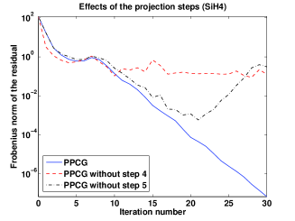
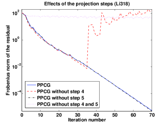
Figure 1: Effects of the projection steps 4 and 5 of Algorithm 2 on convergence. The PPCG variants are applied to compute 10 (left) and 2,000 (right) lowest eigenpairs of the converged Kohn-Sham Hamiltonian of the silane molecule (left) and the Li318 lithium-ion electrolyte (right).

As demonstrated in Figure 1, the PPCG algorithm can be very sensitive to the orthogonal projector used in steps 4 and 5 of Algorithm 2. We observe that removing either of the two projection steps can lead to a severe deterioration of convergence. In Figure 1 (left) the PPCG algorithm is used to compute the 10 lowest eigenpairs of a Kohn-Sham Hamiltonian of the SiH4 (silane) molecule. In Figure 1 (right), a similar computation is performed for the Li318 (lithium-ion electrolyte) system, where $2,000$ eigenpairs are sought.

Interestingly, we observed that the effects of applying $I-XX^{\ast}$ are more pronounced in the cases where $A$ has multiple eigenvalues. Furthermore, in some experiments, we noticed that skipping the projector only in $P$ may not alter the convergence; see Figure 1 (right). Nevertheless, we recommend keeping $(I-XX^{*})$ for computing both $W$ and $P$ to achieve robust convergence.

5.5 Orthogonalization of the approximate invariant subspace

There are a number of ways to obtain an orthonormal basis of $X$ after its columns have been updated by the “for” loop in lines 6-12 of Algorithm 2. If the columns of $X$ are far from being linearly dependent, an orthonormalization procedure based on using the Cholesky factorization of $X^{\ast}X=R^{\ast}R$, where $R$ is a unit upper triangular matrix, is generally efficient. In this case, $X$ is orthonormalized by

$$X\leftarrow XR^{-1},$$

i.e., step 13 of Algorithm 2 is given by the QR decomposition based on the Cholesky decomposition (the Cholesky QR factorization).

If the columns of $X$ are almost orthonormal, as expected when $X$ is near the solution to the trace minimization problem, we may compute the orthonormal basis as $X\leftarrow X(X^{*}X)^{-1/2}$, where $(X^{*}X)^{-1/2}=(I+Y)^{-1/2}$ can be effectively approximated by several terms in the Taylor expansion of $f(x)=\sqrt{1+y}$. This gives the following orthogonalization procedure:

$$X\leftarrow X(I-Y/2+3Y^{2}/8-5Y^{3}/16+\cdots),\quad Y=X^{*}X-I.$$

Since $Y$ is likely to be small in norm, we may only need three or four terms in the above expansion to obtain a nearly orthonormal $X$. An attractive feature of this updating scheme is that it uses only dense matrix–matrix multiplications which can be performed efficiently on modern high performance computers. Note that the updated matrix represents an orthonormal factor in the polar decomposition [22] of $X$, which gives a matrix with orthonormal columns that is closest to $X$ [23].

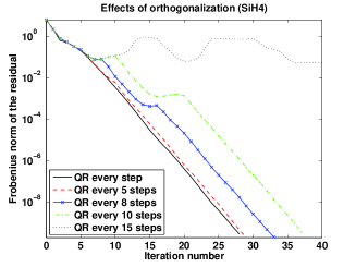
Figure 2: Effects of removing the orthonormalization step 13 of Algorithm 2, when computing the $4$ lowest eigenpairs of a Kohn-Sham Hamiltonian associated with the silane molecule. The problem size is $2,103$.

We have observed that columns of $X$ often remain nearly orthonormal after they are updated according to (10). Motivated by this observation, we experimented with performing orthonormalization periodically (step 13 of Algorithm 2) in the PPCG iteration. Figure 2 demonstrates the effects of this strategy on the convergence of the algorithm. The plotted convergence curves correspond to PPCG runs in which orthonormalization is performed every $t$ steps, where $t=1,5,8,10,15$. In our implementation, we use the Cholesky QR factorization to orthonormalize the columns of $X$.

As can be seen in Figure 2, skipping the QR factorization of $X$ for a small number of PPCG iterations (up to 5 steps in this example) does not affect the convergence of the algorithm. In this case, the loss of orthogonality, which can be measured by $\|X^{*}X-I\|_{F}$, is at most $O(10^{-1})$. Note that when the columns of $X$ are not orthonormal, the projectors in steps 4 and 5 of Algorithm 2 become approximate projectors. Nevertheless, the convergence of PPCG is not substantially affected as long as $t$ is not too large. However, if we reduce the frequency of the QR factorizations significantly, the number of PPCG iterations required to reach convergence starts to increase. For this example, when we perform the QR factorization every $15$ iterations, PPCG fails to converge (within an error tolerance of $10^{-2}$) within 40 iterations. In this case, the loss of orthogonality in $X$ reaches $O(1)$, which severely affects the convergence of the method.

Thus, in order to gain extra computational savings, we can devise an optional heuristic based on the measured loss of orthogonality. We can decide to skip step 13 of Algorithm 2 if the loss of orthogonality is relatively small.

5.6 Periodic RR computation

For many problems, the orthogonal projection of $W$ and $P$ against columns of $X$ and subsequent orthogonalization are not enough to ensure that $X$ converges rapidly to a basis of the desired invariant subspace. We found that a practical remedy for avoiding possible convergence degradation or failure is to perform the RR procedure periodically, which has the effect of systematically repositioning the $j$th column of $X$ towards the eigenvector associated with the $j$th eigenvalue of $A$. In this case, since each column of $X$ is forced to be sufficiently close to an eigenvector, minimizing $k$ Rayleigh quotients separately becomes just as effective as minimizing the trace of $X^{*}AX$ under the orthonormality constraint. Therefore, in practical implementations, we perform RR periodically, even though PPCG has been observed to converge without performing this step for some problems. This is done in step 14 of Algorithm 2.

Another reason periodic RR may be advantageous is that it provides an opportunity to lock converged eigenvectors and reduce the number of sparse matrix vector multiplications required to find the remaining unconverged eigenvectors.

Clearly, introducing the periodic RR calculation increases the cost of some PPCG iterations and can potentially make the algorithm less scalable due to the lack of scalability of the dense eigensolver. However, the extra cost can be offset by accelerated convergence of the algorithm and reduced number of sparse matrix vector multiplications once some approximate eigenvectors have converged. In our PPCG implementation, we control the frequency of the RR calls by a parameter rr_period. Our numerical experiments suggest that a good value of rr_period is between 5 and 10. Because good approximations to desired eigenvectors do not emerge in the first few PPCG iteration, rr_period can be set to a relatively large value and then decreased in later iterations when many converged eigenvector approximations can be found and locked.

5.7 Locking converged eigenvectors

Even before the norm of the subspace residual $R\equiv AX-X(X^{\ast}AX)$ becomes small, some of the Ritz vectors associated with the subspace spanned by columns of $X$ can become accurate. However, these Ritz vectors generally do not reveal themselves through the norm of each column of $R$ because each column of $X$ may consist of a linear combination of converged and unconverged eigenvector approximations. The converged eigenvector approximations can only be revealed through the RR procedure. As mentioned earlier, by performing an RR calculation, we rotate the columns of $X$ to the Ritz vectors which are used as starting points for independent Rayleigh quotient minimization carried out in the inner loop of the next PPCG iteration.

Once the converged Ritz vectors are detected, we lock these vectors by keeping them in the leading columns of $X$. These locked vectors are not updated in inner loop of the PPCG algorithm until the next RR procedure is performed. We do not need to keep the corresponding columns in the $W$ and $P$ matrices. However, the remaining columns in $W$ and $P$ must be orthogonalized against all columns of $X$. This “soft locking” strategy is along the lines of that described in [24].

A detailed description of the PPCG algorithm, incorporating the above practical aspects, is given in Algorithm 3 of Appendix A.

6 Numerical examples

In this section, we give a few examples of how the PPCG algorithm can be used to accelerate both the SCF iteration and the band structure analysis in Kohn-Sham DFT calculations. We implement PPCG within the widely used Quantum Espresso (QE) planewave pseudopotential density functional electronic structure code [8], and compare the performance of PPCG with that of the state-of-the-art Davidson solver implemented in QE. The QE code also contains an implementation of a band-by-band conjugate gradient solver. Its performance generally lags behind that of the Davidson solver, however, especially when a large number of eigenpairs is needed. Therefore, we compare to the Davidson solver here.

In QE, the Davidson algorithm can construct a subspace $Y$ of dimension up to $4k$ before it is restarted. However, when the number of desired eigenpairs $k$ is large, solving a $4k\times 4k$ projected eigenvalue problem is very costly. Therefore, in our tests, we limit the subspace dimension of $Y$ to $2k$.

The problems that we use to test the new algorithm are listed in Table 1. A sufficiently large supercell is used in each case so that we perform all calculations at the $\Gamma$-point only. The kinetic energy cutoff (ecut), which determines the the number of planewave coefficients ($n_{G}$), as well as the number of atoms ($n_{a}$) for each system are shown. Norm conserving pseudopotentials are used to construct the Kohn-Sham Hamiltonian. Therefore, all eigenvalue problems we solve here are standard eigenvalue problems, although our algorithm can be easily modified to solve generalized eigenvalue problems. The local density approximation (LDA) [21] is used for exchange and correlation. The particular choice of pseudopotential and exchange-correlation functional is not important here, however, since we focus only on the performance of the eigensolver.

The distribution of eigenvalues for each problem is plotted in Figure 3. We can see that there are several clusters of eigenvalues for Li318 and bulk Si. They are insulating and semiconducting, respectively. No visible spectral gap can be observed for Graphene512. It is known to be a metallic system. The test cases thus encompass the full range of electronic structures from insulating to metallic.

Problem	$n_{a}$	ecut (Ryd)	$n_{G}$
Li318	318	25	206,691
Graphene	512	25	538,034
bulk Si	1000	35	1,896,173

Table 1: Test problems

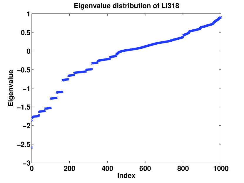
(a) Li318

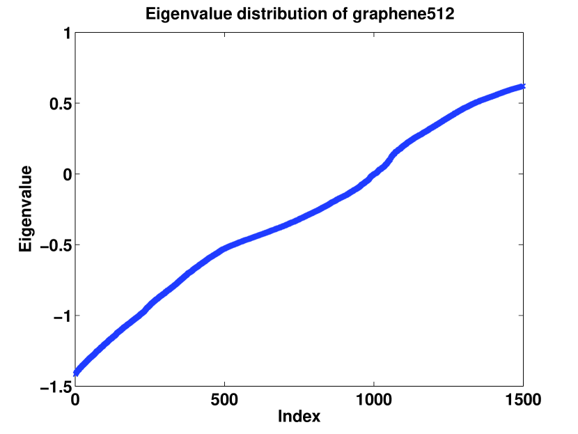
(b) graphene512

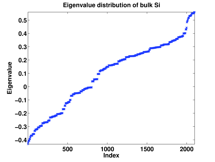
(c) bulk Si

Figure 3: Eigenvalue distributions for test problems.

All tests were performed on Edison, a Cray XC30 supercomputer maintained at the National Energy Research Scientific Computer Center (NERSC) at Lawrence Berkeley National Laboratory. Each node on Edison has two twelve-core Intel 2.4GHz “Ivy Bridge” processor sockets. It is equipped with 64 gigabyte (GB) DDR3 1600MHz shared memory. However, memory access bandwidth and latency are nonuniform across all cores. Each core has its own 64 kilobytes (KB) L1 and 256 KB L2 caches. A 32MB L3 cache is shared among 12 cores. Edison nodes are connected by a Cray Aries network with Dragonfly topology and 23.7 TB/s global bandwidth.

We follow the same parallelization strategy implemented in the QE package to perform the multiplication of the Hamiltonian and a wavefunction and distributed dense matrix–matrix multiplications. The most expensive part of the Hamiltonian and wavefunction multiplication is the three-dimensional FFTs. Each FFT is parallelized over $nz$ cores, where $nz$ is the number of FFT grid points in the third dimension. Multiple FFTs can be carried out simultaneously on different cores when the “-ntg” option is used.

We do not use the multi-threaded feature of QE. The planewave coefficients are partitioned and distributed by rows. Therefore, the dense matrix–matrix multiplications are carried out by calling the DGEMM subroutine in BLAS3 on each processor and performing a global sum if necessarily. The ScaLAPACK library is used to solve the dense projected eigenvalue problem and to perform the Cholesky factorization required in the Cholesky QR factorization. Because ScaLAPACK requires a 2D square processor grid for these computations, a separate communication group that typically consists of fewer computational cores is created to complete this part of the computation. Table 2 gives the default square processor configurations generated by QE when a certain number of cores are used to solve the Kohn-Sham problem. Although we did not try different configurations exhaustively, we found the default setting to be close to optimal, i.e., adding more cores to perform ScaLAPACK calculations generally does not lead to any improvement in timing because of the limited amount of parallelism in dense eigenvalue and Cholesky factorization computations and the communication overhead.

ncpus	Processor grid
200	10x10
400	14x14
800	20x20
1,600	28x28
2,400	34x34
3,000	38x38

Table 2: Default ScaLAPACK processor grid configurations used by QE for different total core counts.

6.1 Band energy calculation

We first show how PPCG performs relative to the Davidson algorithm when they are used to solve a single linear eigenvalue problem defined by converged electron density and its corresponding Kohn-Sham Hamiltonian. Table 3 shows the total wall clock time required by both the block Davidson algorithm and the PPCG algorithm for computing the $k$ lowest eigenpairs of a converged Kohn-Sham Hamiltonian. This is often known as the band structure calculation, although we only compute band energies and corresponding wavefunctions at the $\Gamma$-point of the Brillouin zone.

In all these calculations, we perform the RR procedure every 5 iterations. Depending on the problem, the subblock size sbsize is chosen to be 5 or 50. In our experience, such choice of sbsize leads to satisfactory convergence behavior of the PPCG algorithm (we address this question in more detail below). For all tests, the number of buffer vectors nbuf is set to 50.

Problem	ncpus	$k$	sbsize	Time PPCG	Time Davidson
Li318	480	2,062	5	49 (43)	84 (27)
Graphene512	576	2,254	50	97 (39)	144 (36)
bulk Si	2,400	2,550	50	189 (78)	329 (77)

Table 3: Comparison of the total wall clock time (in seconds) used by PPCG and Davidson to compute the lowest $k$ eigenpairs. Numbers in parentheses correspond to iteration counts.

For both Li318 and Graphene512, we terminate the Davidson iteration when the relative subspace residual norm defined in (11) is less than $tol=10^{-2}$. Since residual norms are only calculated when the Davidson iteration is restarted, the actual residual norm associated with the approximate solution produced by the Davidson algorithm may be much less than $tol$ upon termination. We use that relative residual norm as the stopping criterion for the PPCG algorithm. For bulk Si, we set $tol$ to $10^{-3}$.

The results shown in Table 3 indicate that PPCG performs much better on the test problems than Davidson’s method. We observe almost a factor of two speedup in terms of wall clock time. Note that the number of iterations required by PPCG is noticeably higher than that of Davidson’s method in some cases (e.g., Li318). However, most PPCG iterations are much less expensive than Davidson iterations because they are free of RR calculations. The reduced number of RR calculations leads to better overall performance. As expected, as the sbsize value increases, the difference in total number of outer iterations between PPCG and Davidson becomes smaller. For example, for bulk Si and Graphene512, where sbsize is relatively large ($50$), the number of iterations taken by PPCG and Davidson are almost the same.

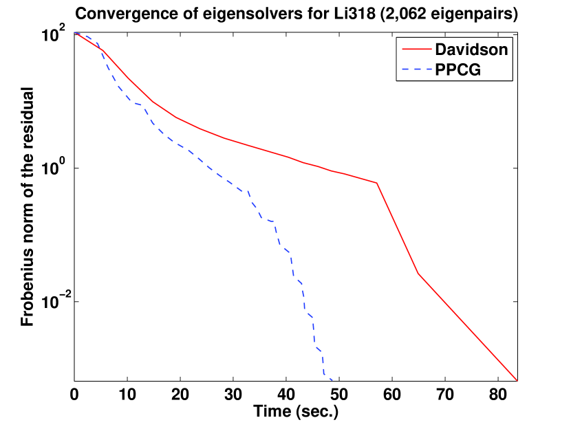
(a) Li318 ($k=2062$)

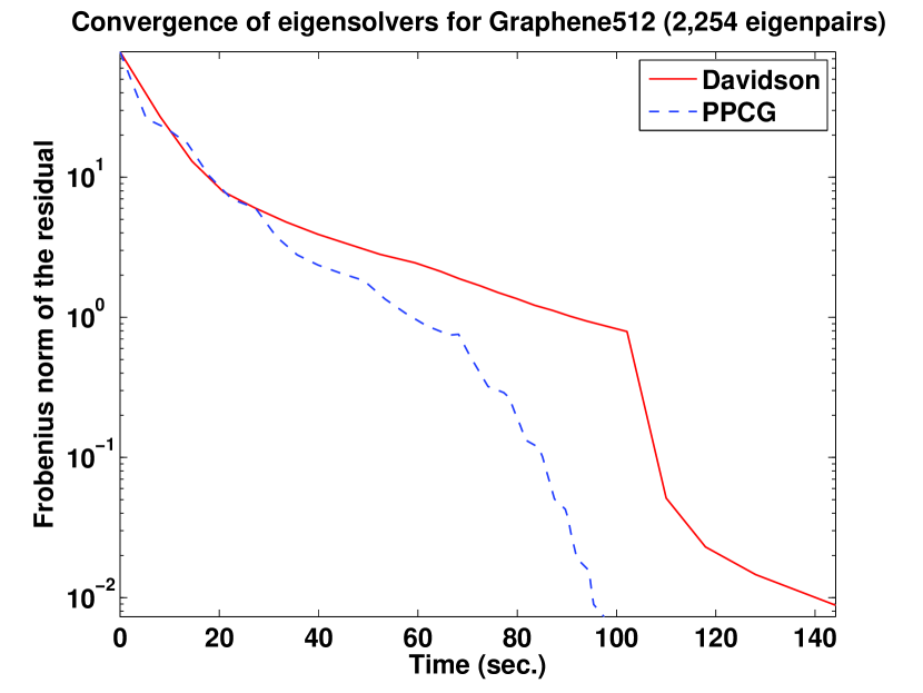
(b) Graphene512 ($k=2254$)

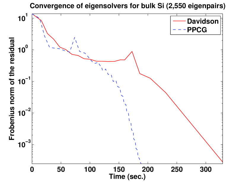
(c) bulk Si ($k=2550$)

Figure 4: Convergence of the Davidson and PPCG algorithms for band structure calculation.

Figure 4 shows how the Frobenius norms of the subspace residuals change with respect to the elapsed time for all three test problems reported in Table 3. Note that at some point, both PPCG and the Davidson method start to converge more rapidly. The change in convergence rate is the result of locking the converged eigenpairs, which significantly reduces computational cost in performing $AX$.

In Tables 4 and 5, we provide a more detailed timing breakdown for both PPCG and Davidson algorithms when they are used to solve Li318 and bulk Si, respectively. We can clearly see that the wall clock time consumed by the Davidson run is dominated by RR calculations. The RR cost is significantly lower in PPCG. However, such a reduction in RR cost is slightly offset by the additional cost of performing Cholesky QR, which we enable in each PPCG iteration. Its cost represents roughly 15% of the total. As has been discussed in Section 5.5, the number of these factorizations can, however, be further reduced, which will lead to even more efficient PPCG.

Computation	PPCG	Davidson
GEMM	16	11
$AX$	10	6
RR	13	66
CholQR	8	0

Table 4: Timing profiles (in seconds) for PPCG and Davidson when they are used to compute the 2,062 lowest eigenpairs of the Li318 problem on 480 cores.

Computation	PPCG	Davidson
GEMM	27	41
$AX$	94	96
RR	40	191
CholQR	19	0

Table 5: Timing profiles (in seconds) for PPCG and Davidson when they are used to compute the 2,550 lowest eigenpairs of the bulk Si problem on 2,400 cores.

We also note from Table 4 that PPCG may spend more time in performing dense matrix–matrix multiplications (GEMM) required to orthogonalize $W$ and $P$ against the current approximation to the desired invariant subspace than the Davidson algorithm. We believe the relatively high cost of GEMM operations is due to the 1D decomposition of the planewave coefficient matrix used in QE, which is less than optimal for machines with many processors. The performance of GEMM depends on the size of the matrices being multiplied on each processor. In the case of Li318, the dimension of the local distributed $X$ is $720\times 2062$, which does not lead to optimal single-processor GEMM performance when $X^{*}X$ or similar matrix–matrix multiplications are computed. For bulk Si, the dimension of the local distributed $X$ is $2024\times 2550$, which is nearly a perfect square. The optimized BLAS on Edison is highly efficient for matrices of this size.

It also appears that PPCG can spend more time in performing $AX$ than the Davidson method. The higher $AX$ cost in PPCG can be attributed to its delayed locking of converged eigenpairs. Because PPCG performs RR periodically, locking must also be performed periodically even though many eigenpairs may have converged before the next RR procedure is called. Although we use a constant RR frequency value rr_period, it is possible to choose it dynamically. In the first few PPCG iterations in which the number of converged eigenvectors is expected to be low, we should not perform the RR procedure too frequently, in order to reduce the RR cost. However, when a large number of eigenvectors start to converge, it may be beneficial to perform the RR procedure more frequently to lock the converged eigenvectors as soon as they appear, and hence reduce the number of sparse matrix multiplications. In our tests, we observe that setting rr_period to a value between 5 and 10 typically yields satisfactory performance.

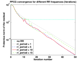
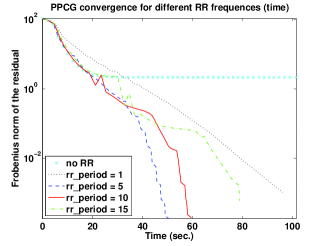
Figure 5: Effect of RR frequency on the convergence of PPCG for the Li318 problem.

In Figure 5, we demonstrate this finding by considering the effects of the RR frequency on the convergence of PPCG in terms of iteration count (left) and time (right) for the Li318 system. We can see that calling the RR procedure periodically is crucial for reaching convergence. Completely removing the RR calculation generally leads to a (near) stagnation of the algorithm. At the same time, it can be seen from Figure 5 (left), that performing the RR procedure too frequently does not necessarily accelerate PPCG convergence. For this particular example, performing RR calculations every 15 iterations in fact results in essentially the same convergence rate as that observed in another PPCG run in which the RR computation is performed at every step.

The effect of the RR frequency becomes more clear when we examine the change of residual norm with respect to the wall clock time. As shown in Figure 5 (right), the best rr_period value for Li318 is 5, i.e., invoking the RR procedure every five steps achieves a good balance between timely locking and reduction of RR computations. As mentioned above, in principle, one can vary the rr_period values during the solution process. As a heuristic, rr_period can be set to a relatively large number in the first several iterations, and then be gradually reduced to provide more opportunities for locking converged eigenvectors. We tried such a strategy for Li318 but did not observe significant improvement. Therefore, we leave rr_period at $5$ in all runs.

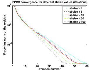
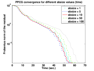
Figure 6: Effect of block size on the convergence of PPCG for the Li318 problem.

Figure 6 shows the effect of the block size sbsize on PPCG convergence for the Li318 problem. One can see that increasing the sbsize value results in a smaller number of iterations required to achieve the desired tolerance (Figure 6, left). This behavior is expected, because in the limiting case where sbsize$=k$, PPCG becomes the LOBPCG method, which optimizes in the full $3k\times 3k$ subspace in each iteration.

Figure 6 (right) demonstrates the effect of sbsize on the solution time. Remarkably, a larger block size, which leads to a reduced iteration count, does not necessarily result in better overall performance, even though it tends to reduce outer iterations. This is in part due to the sequential implementation of the for loop in step 11 in the current implementation. Since each block minimization in the inner loop can take a non-negligible amount of time, the inner for loop can take a significant amount of time, even though the loop count is reduced. On the other hand, setting sbsize$=1$ is not desirable either, because of that tends to slow convergence and increase the outer PPCG iteration count. Furthermore, the inner minimization cannot effectively take advantage of BLAS3 operations in this case. For Li318, we observe that the best sbsize value is $5$.

In Figure 7, we plot how the wall clock times of PPCG and Davidson change with respect to the number of cores when applied to the Li318 and bulk Si problems.

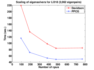
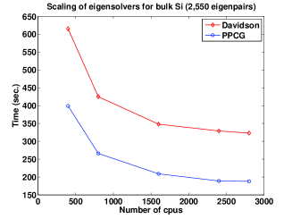
Figure 7: Scaling of the Davidson and PPCG algorithms when used to compute $2,062$ and $2,550$ bands of the converged Kohn-Sham Hamiltonian of the Li318 (left) and bulk Si (right) systems, respectively.

We observe that both algorithms exhibit nearly perfect parallel scalability when a relatively small number of cores are used in the computation. However, as the number of cores increases, the performance of both algorithms stagnates.

	ncpus
Computation	48	96	192	384	480	768
GEMM	77	44	26	18	16	16
$AX$	33	28	17	13	10	11
RR	40	24	16	13	13	13
CholQR	28	16	9	8	8	9
Total	186	116	71	53	49	50

Table 6: Scaling of different computational components of PPCG for Li318.

	ncpus
Computation	48	96	192	384	480	768
GEMM	54	29	17	12	11	11
$AX$	22	19	13	8	6	7
RR	370	170	105	77	66	66
Total	449	219	136	98	84	85

Table 7: Scaling of different computational components of the Davidson algorithm for Li318.

A closer look at the timing profiles consisting of wall clock time used by different computational kernels, as shown in Tables 6–9, reveals that the lack of scalability at high core count is caused by the poor parallel scaling of both $AX$ and $GEMM$ calculations at such core counts. A similar picture is observed for other cases we have tested.

	ncpus
Computation	200	400	800	1,600	2,400	2,800
GEMM	202	104	57	35	27	26
$AX$	247	165	129	106	94	92
RR	142	77	48	40	40	41
CholQR	66	91	21	18	19	21
Total	685	399	266	209	189	188

Table 8: Scaling of different computational components of PPCG for bulk Si.

	ncpus
Computation	200	400	800	1,600	2,400	2,800
GEMM	248	138	76	47	41	38
$AX$	253	169	133	111	96	96
RR	474	303	214	189	191	189
Total	986	615	425	348	329	323

Table 9: Scaling of different computational components of Davidson’s algorithm for bulk Si.

The less than satisfactory scalability of GEMM is likely due to the 1D partition of the planewave coefficients in QE. We are aware of a recent change in the QE design to allow planewave coefficients to be distributed on a 2D processor grid such as the one used in ABINIT [25, 26, 27] and Qbox [28]. However, the new version of the code is still in the experimental stage at the time of this writing. Hence we have not tried it. Once the new version of QE becomes available, we believe the benefit of using PPCG to compute the desired eigenvectors will become even more substantial.

The poor scalability of $AX$ is due to the overhead related to the all-to-all communication required in 3D FFTs. When a small number of cores are used, this overhead is relatively insignificant due to the relatively large ratio of computational work and communication volume. However, when a large number of cores are used, the amount of computation performed on each core is relatively low compared to the volume of communication. We believe that one way to reduce such overhead is to perform each FFT on fewer than $n_{z}$ cores, where $n_{z}$ is the number of FFT grid point in the third dimension. However, this would require a substantial modification of the QE software.

6.2 SCF calculation

We ran both the block Davidson (Algorithm 1) and the new PPCG algorithm to compute the solutions to the Kohn-Sham equations for the three systems list in Table 1. To account for partial occupancy at finite temperature, we set the number of bands to be computed to $k=886$ for Li318; $k=1,229$ for Graphene512; and $k=2,000$ for bulk Si.

In general, it is not necessary to solve the linear eigenvalue problem to high accuracy in the first few SCF cycles because the Hamiltonian itself has not converged. As the electron density and Hamiltonian converge to the ground state solution, we should gradually demand higher accuracy in the solution to the linear eigenvalue problem. However, because the approximate invariant subspace obtained in the previous SCF iteration can be used as a good starting guess for the eigenvalue problem produced in the current SCF iteration, the number of Davidson iterations required to reach high accuracy does not necessarily increase. The QE implementation of Davidson’s algorithm uses a heuristic to dynamically adjust the convergence tolerance of the approximate eigenvalues as the electron density and Hamiltonian converge to the ground-state solution. In most cases, the average number of Davidson iterations taken in each SCF cycle is around 2. We have not implemented the same heuristic for setting a dynamic convergence tolerance partly because we do not always have approximate eigenvalues. To be comparable to the Davidson solver, we simply set the maximum number of iterations allowed in PPCG to 2. In all our test cases, two PPCG iterations were taken in each SCF cycle.

Problem	ncpus	sbsize	PPCG	Davidson
Li318	480	5	35 (40)	85 (49)
Graphene512	576	10	103 (54)	202 (57)
bulk Si	2,000	5	218 (14)	322 (14)

Table 10: Comparison of total wall clock time (in seconds) used by PPCG and Davidson algorithms to compute solutions of the Kohn-Sham equations. Numbers in parentheses correspond to SCF iteration counts.

In Table 10, we report the overall time used in both the Davidson and PPCG versions of the SCF iteration for all three test problems. The SCF convergence tolerance, which is used to terminate the SCF iteration when the estimated total energy error predicted by the so-called Harris–Foulkes energy functional [Har85, FouHay89] is sufficiently small, is set to $10^{-6}$ for Li318 and bulk Si. It is set to $10^{-4}$ for Graphene512 because the SCF iteration converges more slowly for this problem, hence takes much longer to run. Note that the SCF convergence tolerance is defined internally by QE, which we did not modify. Thus both the Davidson and PPCG versions of the SCF iteration are subject to the same SCF convergence criterion. We also use the same (“plain”) mixing and finite temperature smearing in both the Davidson and PPCG runs. Note that, following the discussion in section 5.5, we omit the Cholesky QR step in PPCG for the reported runs. Since only two eigensolver iterations are performed per SCF iteration, this did not affect convergence and resulted in a speedup of the overall computation. The sbsize parameter has been set to $5$ for the Li318 and bulk Si systems, and to 10 for Graphene512.

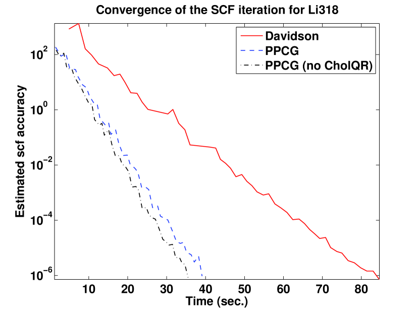
(a) Li318

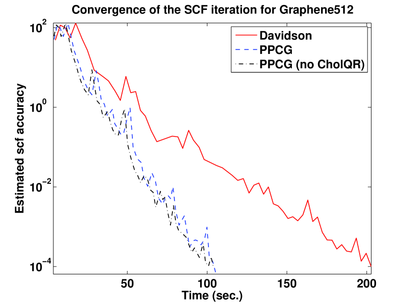
(b) Graphene512

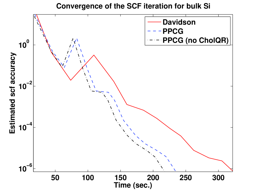
(c) bulk Si

Figure 8: Convergence of the SCF iteration with Davidson and PPCG algorithms.

The convergence curves corresponding to the SCF runs of Table 10 are shown in Figure 8. We can clearly see that the PPCG based SCF iteration can be nearly twice as fast as the Davidson based iteration. The figure also demonstrates the effects of skipping the Cholesky QR step, which further reduces the PPCG run time. It appears that, for the Li318 and Graphene512 examples, a slightly fewer number of SCF iterations is needed to reach convergence when PPCG is used to solve the linear eigenvalue problem in each step.

In Figure 9, we compare scalability of the SCF iteration based on the PPCG (without Cholesky QR) and Davidson algorithms. We report the results for Li318 (left) and bulk Si (right). Similar to the case of the band structure calculations, both schemes scale approximately up to the same number of cores for Li318, whereas scalability of PPCG is slightly better for the bulk Si example.

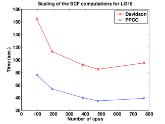
Figure 9: Scaling of SCF iterations with the Davidson and PPCG algorithms for Li318 (left) and bulk Si (right) systems.

7 Conclusions

We presented a projected preconditioned conjugate gradient (PPCG) algorithm for computing an invariant subspace associated with the smallest eigenvalues of a large Hermitian matrix. The key feature of the new algorithm is that it performs fewer Rayleigh-Ritz computations, which are often the bottleneck in iterative eigensolvers when the number of required eigenpairs is relatively large (e.g., over thousands). We discussed a number of practical issues that must be addressed in order to implement the algorithm efficiently.

We implemented the PPCG algorithm within the widely used Quantum Espresso (QE) planewave pseudopotential electronic structure software package. We demonstrated that PPCG is nearly two times faster than the existing state-of-the-art Davidson algorithm implemented in QE for a number of test problems. We believe further performance gains can be achieved in PPCG relative to other algorithms if the multiplication of $A$ with a block of vectors $X$ and the dense matrix multiplications such as $X^{\ast}X$ are implemented in a scalable fashion.

Acknowledgments.

The authors thank Dr. Erik Draeger at the Lawrence Livermore National Laboratory for insightful comments and discussions.

Appendix A Detailed description of the PPCG algorithm

In this appendix, we summarize the practical aspects related to implementation of PPCG, discussed in Section 5, in Algorithm 3. Note that if storage for $AX$, $AW$, and $AP$ is available, then the method can be implemented using one matrix–block multiplication and one block preconditioning operation per iteration. If only an invariant subspace is needed on output, then the last step of the algorithm can be omitted.

Input: The matrix $A$, a preconditioner $T$, a starting guess of the invariant subspace $X^{(0)}\in\mathbb{C}^{n\times k}$ associated with the $k$ smallest eigenvalues of $A$, $X^{(0)*}X^{(0)}=I$, parameter rr_period to control the RR frequency, the splitting parameter sbsize, and the number nbuf of buffer vectors; Output: Approximate eigenvectors $X\in\mathbb{C}^{n\times k}$ associated with the $k$ smallest eigenvalues $\Lambda$ of $A$; 1:  $X\leftarrow X^{(0)}$; $X_{\text{lock}}\leftarrow\left[\ \right]$; $P\leftarrow\left[\ \right]$; $\text{iter}\leftarrow 1$; 2:  Add nbuf buffer vectors to $X$, $k\leftarrow k+$nbuf; $k_{\text{act}}\leftarrow k$; 3:  Initialize index sets $J=\{1,\ldots,k\}$ and $J_{\text{lock}}\leftarrow\left[\ \right]$; 4:  Compute the initial subspace residual $W\leftarrow AX-X(X^{*}AX)$; 5:  Use sbsize to determine the number $s$ of subblocks. 6:  Define the splitting $X=[X_{1},\ \ldots,\ X_{s}]$ and $W=[W_{1},\ \ldots,\ W_{s}]$. 7:  while convergence not reached  do 8:     $W\leftarrow TW$; 9:     $W\leftarrow(I-XX^{*})W$ and $W\leftarrow(I-X_{\text{lock}}X_{\text{lock}}^{*})W$; 10:     $P\leftarrow(I-XX^{*})P$ and $P\leftarrow(I-X_{\text{lock}}X_{\text{lock}}^{*})P$; 11:     for $j=1,\ldots,s$ do 12:        $S\leftarrow[X_{j},W_{j},P_{j}]$ ($P_{j}=0$ if $P=[\ ]$); 13:        Find eigenvectors $C=[C_{X},\ C_{W},\ C_{P}]^{T}$ ($C_{P}=0$ if $P=\left[\ \right]$) associated with the $k$ smallest eigenvalues $\Omega$ of (3); 14:        $P_{j}\leftarrow W_{j}C_{W}+P_{j}C_{P}$; 15:        $X_{j}\leftarrow X_{j}C_{X}+P_{j}$; 16:     end for 17:     if $\text{mod}(\text{iter},\text{rr\_period} )\neq 0$ then 18:        Compute Cholesky factorization $X^{*}X=R^{*}R$; 19:        $X\leftarrow XR^{-1}$; 20:        $W\leftarrow AX-X(X^{*}AX)$; 21:     else 22:        Set $S=[X,\ X_{\text{lock}}]$; 23:        Find eigenvectors $C$ associated with the $k$ smallest eigenvalues $\Omega$ of (3); 24:        $X\leftarrow SC$; $\Lambda\leftarrow\Omega$; 25:        $W\leftarrow AX-X\Lambda$; 26:        Use $W$ to determine column indices $J_{\text{lock}}$ of $X$ that correspond to converged eigenpairs; define the indices of active columns $J_{\text{act}}\leftarrow J\setminus J_{\text{lock}}$; 27:        $X_{\text{lock}}\leftarrow X(J_{\text{lock}})$; 28:        $X\leftarrow X(J_{\text{act}})$; $W\leftarrow W(J_{\text{act}})$; $P\leftarrow P(J_{\text{act}})$; 29:        Set $k_{\text{act}}$ to the number of active columns; 30:        Compute the number $s$ of subblocks for splitting the active columns (similar to step 5); 31:        Define the splitting of active columns $X=[X_{1},\ \ldots,\ X_{s}]$, $W=[W_{1},\ \ldots,\ W_{s}]$, and $P=[P_{1},\ \ldots,\ P_{s}]$. 32:     end if 33:     $\text{iter}\leftarrow\text{iter}+1$; 34:  end while 35:  Perform steps 22-24 to obtain final eigenpair approximations ($X,\Lambda$).

Algorithm 3 The PPCG algorithm (detailed description of Algorithm 2)

References

- [1] Y. Saad, Numerical Methods for Large Eigenvalue Problems- classics edition, SIAM, Philadelpha, PA, 2011.
- [2] E. R. Davidson, The iterative calculation of a few of the lowest eigenvalues and corresponding eigenvectors of large real symmetric matrices, J.. Comput. Phys. 17 (1) (1975) 87–94.
- [3] A. Knyazev, Toward the optimal preconditioned eigensolver: Locally Optimal Block Preconditioned Conjugate Gradient method, SIAM J. Sci. Comput. 23 (2) (2001) 517–541.
- [4] L. S. Blackford, J. Choi, A. Cleary, E. D’Azevedo, J. Demmel, I. Dhillon, J. Dongarra, S. Hammarling, G. Henry, A. Petitet, K. Stanley, D. Walker, R. C. Whaley, ScaLAPACK Users’ Guide, Society for Industrial and Applied Mathematics, Philadelphia, PA, 1997.
- [5] G. Schofield, J. R. Chelikowsky, Y. Saad, A spectrum slicing method for the Kohn–Sham problem, Comput. Phys. Commun. 183 (3) (2012) 497–505.
- [6] Z. Wen, C. Yang, X. Liu, Y. Zhang, Trace penalty minimization for large-scale eigenspace computation, Tech. Rep. 13-03, Rice University, submitted to J. Sci. Comp. (2013).
- [7] W. J. Stewart, A. Jennings, A simultaneous iteration algorithm for real matrices, ACM Trans. Math Softw. (TOMS) 7 (1981) 184–198.
-
[8]
P. Giannozzi, S. Baroni, N. Bonini, M. Calandra, R. Car, C. Cavazzoni,
D. Ceresoli, G. L. Chiarotti, M. Cococcioni, I. Dabo, A. Dal Corso,
S. de Gironcoli, S. Fabris, G. Fratesi, R. Gebauer, U. Gerstmann,
C. Gougoussis, A. Kokalj, M. Lazzeri, L. Martin-Samos, N. Marzari, F. Mauri,
R. Mazzarello, S. Paolini, A. Pasquarello, L. Paulatto, C. Sbraccia,
S. Scandolo, G. Sclauzero, A. P. Seitsonen, A. Smogunov, P. Umari, R. M.
Wentzcovitch, Quantum espresso: a
modular and open-source software project for quantum simulations of
materials, Journal of Physics: Condensed Matter 21 (39) (2009) 395502
(19pp).
URL http://www.quantum-espresso.org - [9] A. Marek, V. Blum, R. Johanni, V. Havu, B. Lang, T. Auckenthaler, A. Heinecke, H.-J. Bungartz, H. Lederer, The ELPA library: scalable parallel eigenvalue solutions for electronic structure theory and computational science, J. Phys.: Condens. Matter 26 (21) (2014) 213201.
- [10] J. Poulson, B. Marker, R. van de Geijn, J. Hammond, N. Romero, Elemental: A new framework for distributed memory dense matrix computations, ACM Trans. Math. Softw. 39 (2) (2013) 13:1–13:24.
- [11] A. Sameh, J. A. Wisniewski, A trace minimization algorithm for the generalized eigenvalue problem, SIAM J. Numer. Anal. 19 (1982) 1243–1259.
- [12] A. Sameh, Z. Tong, The trace minimization method for symmetric generalized eigenvalue problem, Journal of Computational and Applied Mathematics 123 (2000) 155–175.
- [13] R. T. Haftka, Z. Gürdal, Elements of Structural Optimization, 3rd Edition, Kluwer Academic Publishers, 1992.
- [14] J. Nocedal, S. Wright, Numerical Optimization, Springer Series in Operations Research, Springer, 1999.
- [15] B. T. Polyak, Introduction to Optimization, Translations Series in Mathematics and Engineering, Optimization Software, 1987.
- [16] E. S. Levitin, B. T. Polyak, Constrained minimization methods, Zh. Vychisl. Mat. Mat. Fiz. 6 (5) (1966) 1–50.
- [17] A. A. Goldstein, Convex programming in Hibert space, Bull. Amer. Math. Soc. 70 (1964) 709–710.
- [18] J. B. Rosen, The gradient projection method for nonlinear programming. Part i. Linear constraints, J. Soc. Indust. Appl. Math. 8 (1) (1960) 181–217.
- [19] J. B. Rosen, The gradient projection method for nonlinear programming. Part ii. Nonlinear constraints, J. Soc. Indust. Appl. Math. 9 (4) (1961) 514–532.
- [20] P. Hohenberg, W. Kohn, Inhomogeneous electron gas, Phys. Rev. 136 (1964) B864–B871.
- [21] W. Kohn, L. Sham, Self-consistent equations including exchange and correlation effects, Phys. Rev. 140 (1965) A1133–A1138.
- [22] R. A. Horn, C. R. Johnson, Matrix Analysis, Cambridge University Press, New York, 1985.
- [23] K. Fan, A. J. Hoffman, Some metric inequalities in the space of matrices, Proc. Amer. Math. Soc. 6 (1955) 111–116.
- [24] A. V. Knyazev, M. E. Argentati, I. Lashuk, E. E. Ovtchinnikov, Block locally optimal preconditioned eigenvalue xolvers (BLOPEX) in hypre and PETSc, SIAM Journal on Scientific Computing 25 (5) (2007) 2224–2239.
- [25] X. Gonze, B. Amadon, P.-M. Anglade, J.-M. Beuken, F. Bottin, P. Boulanger, F. Bruneval, D. Caliste, R. Caracas, M. Cote, T. Deutsch, L. Genovese, P. Ghosez, M. Giantomassi, S. Goedecker, D. Hamann, P. Hermet, F. Jollet, G. Jomard, S. Leroux, M. Mancini, S. Mazevet, M. Oliveira, G. Onida, Y. Pouillon, T. Rangel, G.-M. Rignanese, D. Sangalli, R. Shaltaf, M. Torrent, M. Verstraete, G. Zerah, J. Zwanziger, ABINIT:First-principles approach of materials and nanosystem properties, Computer Phys. Commun. 180 (2009) 2582–2615.
- [26] X. Gonze, G.-M. Rignanese, M. Verstraete, J.-M. Beuken, Y. Pouillon, R. Caracas, F. Jollet, M. Torrent, G. Zerah, M. Mikami, P. Ghosez, M. Veithen, J.-Y. Raty, V. Olevano, F. Bruneval, L. Reining, R. Godby, G. Onida, D. Hamann, D. Allan, A brief introduction to the ABINIT software package, Allan. Zeit. Kristallogr. 220 (2005) 558–562.
- [27] F. Bottin, G. Z. S. Leroux, A. Knyazev, Large scale ab initio calculations based on three levels of parallelization, Computational Material Science 42 (2) (2008) 329–336.
- [28] F. Gygi, Architecture of Qbox: a scalable first-principles molecular dynamics code, IBM Journal of Research and Development 52 (1/2) (2008) 137–144.