Simulating Flexible Fiber Suspensions using a Scalable Immersed Boundary Algorithm

Abstract

We present an approach for numerically simulating the dynamics of flexible fibers in a three-dimensional shear flow using a scalable immersed boundary (IB) algorithm based on Guermond and Minev’s pseudo-compressible fluid solver. The fibers are treated as one-dimensional Kirchhoff rods that resist stretching, bending, and twisting, within the generalized IB framework. We perform a careful numerical comparison against experiments on single fibers performed by S. G. Mason and co-workers, who categorized the fiber dynamics into several distinct orbit classes. We show that the orbit class may be determined using a single dimensionless parameter for low Reynolds flows. Lastly, we simulate dilute suspensions containing up to hundreds of fibers using a distributed-memory computer cluster. These simulations serve as a stepping stone for studying more complex suspension dynamics including non-dilute suspensions and aggregation of fibers (also known as flocculation).

siscxxxxxxxx–x

1 Introduction

The behaviour of long, flexible fibers in a suspension plays an important role in many applications, including pulp and paper manufacture, polymer melts, and fiber-reinforced composite materials [21, 46]. The dynamics of such suspensions depend heavily on the shape and flexibility of the individual fibers as well as the interactions between fibers. Because of the complexity of the fiber motion in suspensions, many researchers have developed numerical methods that afford valuable insight into both individual fiber dynamics and the resulting aggregate suspension rheology [20, 37, 46]. These simulations can complement physical experiments by providing information that is not easily obtained through direct measurement.

In this paper, we develop an approach for simulating a suspension of flexible fibers that is based on the immersed boundary (IB) method [36], which is a mathematical framework originally developed by Peskin [35] to capture the two-way interaction between a fluid and an immersed deformable structure. Here, the fluid deforms the elastic structure while the structure exerts forces onto the fluid. The IB method has been used to study a wide variety of biological and engineering applications including blood flow through heart valves [13, 35], cell growth and deformation [38], jellyfish locomotion [17], evolution of dry foams [24] and parachute aerodynamics [23].

We treat the flexible fibers as one-dimensional Kirchhoff rods [7] described using the generalized IB framework developed by Lim et al. [28]. In this approach, the fibers are represented as 1D space curves using a moving Lagrangian coordinate, wherein at each Lagrangian point an orthonormal triad of vectors describes the orientation and “twist state” of the rod. This permits the fiber to generate not only a force but also a torque that is applied to the surrounding fluid.

The primary objective of this paper is to develop an efficient methodology for simulating suspensions containing a large number of flexible fibers. Since solving the full fluid-structure interaction problem comes at the expense of additional computational work, the underlying parallel algorithm is purposely designed to scale efficiently on distributed-memory computer clusters. This permits non-dilute suspensions to be simulated efficiently by spreading the work over multiple processors. The numerical algorithm is based on the work of Wiens and Stockie [53] who implemented a pseudo-compressible fluid solver developed by Guermond and Minev [15, 16] in the IB framework. We extend this original algorithm to use the Eulerian–Lagrangian discretization employed by Griffith and Lim [12] which employs a predictor-corrector procedure to evolve the immersed boundary. Here, two separate force spreading and velocity interpolation steps are applied at each time step which improves the spatial convergence rate of the method.

We begin in Section 2 by reviewing theoretical and experimental results in the literature pertaining to the hydrodynamics of suspensions containing flexible fibers, as well as discussing several prominent computational approaches. In Sections 3 and 4, we state the governing equations underlying our IB model for fluid-fiber interaction, as well as the numerical algorithm used to approximate these equations. In Section 5, we present simulations of fiber dynamics in both single- and multi-fiber systems, and compare these results to previously published experimental work.

2 Background: Pulp Fibers

2.1 Theory and Experiments

Theoretical investigations of the dynamics of fibers in a shear flow date back to Jeffery in the 1920s [19], who derived an analytical solution for the motion of a single rigid, neutrally-buoyant ellipsoidal particle immersed in an incompressible Newtonian fluid (specifically, in a Stokes flow). Jeffery found that such a fiber rotates with a well-defined periodic orbit having constant period but non-uniform angular velocity. It was later shown by Bretherton [3] that Jeffery’s analytical solution could be extended to more general axisymmetric particles with non-elliptical cross-sections by replacing the ellipsoidal aspect ratio $a_{r}$ by an effective aspect ratio $a_{r}^{\ast}$.

Although the theory for rigid fiber dynamics is relatively well-developed, far less is known about fibers that experience significant bending. For this reason, experimental observations are of critical importance in understanding the dynamics and rheology of suspensions containing flexible fibers. Unlike rigid fibers, flexible fibers undergo a much wider and richer range of motion when subjected to a background linear shear flow given with velocity field $\boldsymbol{u}=(Gy,0,0)$. This problem was studied in the pioneering work of Mason and co-workers [1, 10, 11] who categorized the fiber dynamics into several distinct orbit classes. When motions are confined to the $xy$-plane, fiber dynamics fall into one of four orbit classes – rigid, springy, flexible, and complex rotations – which are illustrated in Table 1. The experiments of Mason et al. involved primarily synthetic fibers (made of rayon and dacron) immersed in highly viscous fluids (such as corn syrup) although their original motivation was the application to natural wood pulp fiber suspensions.

Table 1: Two-dimensional orbit classes for flexible fibers whose unstressed state is intrinsically straight. Adapted from Forgacs et al. [11].

	Orbit Class
I	Rigid rotation
II	Springy rotation
IIIa	Loop or S turn
IIIb	Snake turn
IV	Complex rotation

These experiments on fiber suspensions demonstrate that varying either the hydrodynamic drag force or the fiber flexibility governs the transition between the various planar orbit classes. In class I orbits, the fiber remains rigid and rotates as predicted by Jeffery’s equation. When a small flexibility is introduced into the fiber, it undergoes a springy rotation (class II) in which it bends into a shallow arc as it rotates outside the horizontal plane of shear. When the fiber flexibility is increased, it experiences significant deformations that take the form of S turns (class IIIa) or snake turns (class IIIb). Note that S turns require a high degree of initial symmetry so that snake turns are actually far more prevalent in actual suspensions [1, 10]. When the fiber flexibility is increased even further, the fiber may never straighten out as it returns to the horizontal, in which case the orbit is classified as a complex rotation (class IV). For the largest values of flexibility encountered in thread-like synthetic fibers, the fiber can transition beyond the class of complex rotations and undergo convoluted self-intersections as observed by Forgacs and Mason [10] in experiments.

In many cases, the fiber rotation is not constrained to the $xy$-plane but instead undergoes a genuinely three-dimensional orbit that protrudes or “buckles” out along the $z$-direction, although the $xy$-projection of the fiber may still belong to one of the planar orbit classes I–IV described above. Note that real suspensions such as wood pulp also contain irregularly-shaped fibers that are either intrinsically curved or contain kinks or other non-uniformities; consequently, fiber orbital dynamics in such suspensions are not necessarily confined to these idealized orbit classes. Indeed, the experiments of Arlov et al. [1] were used to classify a much broader class of genuinely three-dimensional orbits for wood pulp fibers having an intrinsic curvature.

We close this discussion by defining a dimensionless parameter that can be used to conveniently classify and predict the orbit class to which a specific fiber belongs. For low Reynolds number flows (with $\mbox{Re}\lessapprox 1$), the hydrodynamic drag force experienced by a fiber is proportional to

(1) $$F_{d}=\mu GD,$$

where $\mu$ is the fluid viscosity, $G$ is the shear rate, and $D$ is the diameter of the fiber [51]. By balancing this drag force with the corresponding fiber bending force, a single dimensionless parameter can be derived that captures the fiber flexibility [42]

(2) $$\chi=\frac{\mu DGL^{3}}{EI},$$

where $L$ is the fiber length, $E$ is Young’s modulus of the material, and $I$ is moment of area in the plane of bending. The parameter $\chi$ may also be interpreted as a ratio of fiber deflection to fiber length. In a series of 2D numerical simulations [44], the parameter $\chi$ was shown to provide a useful measure of fiber flexibility that characterizes each orbit class over a wide range of fluid and fiber parameters. This dimensionless flexibility parameter has also appeared in the computational studies of Ross and Klingenberg [39] (where they referred to it as a dimensionless shear rate) and Wherrett et al. [50] (where $\chi^{-1}$ is called a bending number).

2.2 Overview of Computational Approaches

A popular class of numerical methods for simulating flexible fibers is the so-called bead models in which a flexible fiber is treated as a string of rigid beads that are linked together by flexible connectors. This approach originated with the work of Yamamoto and Matsuoka [56] who treated fibers as chains of bonded spheres that are free to stretch, bend and twist relative to each other. Their approach was extended by Ross and Klingenberg [39] who modelled fibers as chains of rigid prolate spheroids connected by ball and socket joints. The dynamics of the bead network are governed by Newton’s laws through a balance of linear and angular momentum that incorporates the hydrodynamic and interparticle forces acting on each bead. More recently, Klingenberg’s group has validated their model results against experiments for single fiber dynamics [41] as well as developing a multi-fiber extension that has been used to simulate flocculation [45].

A significant shortcoming of Klingenberg’s model and related variants [48, 50, 56] is that they fail to capture the full fluid-structure interaction in fiber suspensions. Although their approach does include the hydrodynamic force exerted by the fluid on the fiber, the fiber does not itself exert any force back onto the fluid; therefore, the fluid is a passive medium that obviously neglects any of the complex fluid dynamics that must occur in the region immediately adjacent to a dynamically deforming fiber. Several recent bead-type models have attempted to address this limitation, for example Wu and Aidun who proposed a model for rigid [55] and flexible [54] fibers that incorporates the full fluid-structure interaction using a Lattice Boltzmann approach. Similarly, Lindström and Uesaka proposed an alternative model for rigid [31] and flexible [29, 30] fibers that uses the incompressible Navier–Stokes equations to model the fluid.

A completely different approach for capturing flexible fiber dynamics is based on the slender body theory [2] which exploits approximations to the governing equations based on a small fiber aspect ratio. This is the approach taken by Tornberg and Shelley [47] who studied flexible filaments in a Stokes flow by deriving a system of one-dimensional integral equations. They solved these integral equations numerically using a second-order method that also captures interactions between multiple fibers. This approach has been further extended by Li et al. [26] who used a similar methodology to investigate the problem of sedimentation (or settling) of flexible fibers. Unlike the bead models described earlier, this slender-body approach cleanly separates the fiber model from its numerical treatment, which makes the model more amenable to mathematical analysis and also permits the numerical discretization to be independently tested through convergence studies. Furthermore, because the fluid has been simplified by assuming a Stokes flow regime, these slender-body discretizations do not require a fluid grid because of the availability of numerical methods based on Green’s-function solutions that greatly reduce the computational complexity. The only significant disadvantage of this approach, beside the Stokes flow restriction, is that there are as yet no results that incorporate any effects of fiber twist [34].

An alternative approach that permits simulating flexible fibers immersed in higher Reynolds flows is the immersed boundary method. This is the approach taken by Stockie and Green [44] who simulated a single flexible fiber in two dimensions using a simple representation of the fiber in terms of spring-like forces that resist stretching and bending. Stockie [43] later extended these results to a single 3D wood pulp fiber using a much more detailed and realistic model that explicitly captures the interwoven multi-layer network of cellulose fibrils making up the wood cell wall. More recently, Nguyen and Fauci studied diatom chains using the IB method with a similarly detailed fiber model [33]. The IB method properly captures the full interaction between the fluid and immersed structure by including the appropriate no-slip boundary condition along the fiber, although it does come at an additional cost. First of all, in comparison with slender-body models, the fluid solver portion of the IB algorithm can be significantly more expensive because it solves the Navier-Stokes equations on a finite difference grid. Secondly, because the IB method aims to capture the detailed fluid flow around the fiber, the fluid grid needs to be adequately refined in order to resolve details on the order of the fiber diameter, which in turn places practical limitations on the fiber aspect ratio that can be computed. Thirdly, a detailed characterization of the structure of a three-dimensional fiber such as in [33, 43] typically requires thousands of IB points to resolve and is therefore computationally impractical for simulating semi-dilute suspensions of multiple fibers.

In this paper, we apply the IB approach to simulate flexible fibers, and we have chosen to treat each fiber instead as a one-dimensional Kirchhoff rod that resists stretching, bending and twisting, as described in the generalized IB method of Lim et al. [28]. Additionally, we employ a highly scalable implementation of the generalized IB algorithm [53] that spreads the computational work over a large number of processors, thereby permitting us to simulate hydrodynamic interactions in suspensions containing large numbers of flexible fibers.

3 Governing Equations

Consider a Newtonian, incompressible fluid that fills a rectangular domain $\Omega$ having dimensions $H_{x}\times H_{y}\times H_{z}$ and whose state is specified using Eulerian coordinates $\boldsymbol{x}=(x,y,z)$. Immersed within the fluid is a neutrally-buoyant elastic fiber of length $L$. The fiber is described by a one-dimensional space curve $\Gamma\subset\Omega$, parameterized by the Lagrangian coordinate $s\in[0,L]$. The spatial configuration of the rod at time $t$ is given in parametric form as $\boldsymbol{x}=\boldsymbol{X}(s,t)$ and its orientation and “twist state” are defined in terms of the orthonormal triad of vectors $\{\boldsymbol{D}^{1}(s,t),\boldsymbol{D}^{2}(s,t),\boldsymbol{D}^{3}(s,t)\}$, where the third triad vector $\boldsymbol{D}^{3}$ remains tangent to the space curve $\boldsymbol{X}$. Note that because of numerical considerations (described shortly), $\boldsymbol{D}^{3}(s,t)$ is not exactly tangent to the space curve $\boldsymbol{X}$ but is rather penalized in a way that it is only approximately in the tangential direction.

The fluid velocity $\boldsymbol{u}(\boldsymbol{x},t)$ and pressure $p(\boldsymbol{x},t)$ at location $\boldsymbol{x}$ and time $t$ are governed by the incompressible Navier–Stokes equations

(3) $$\rho\left(\frac{\partial\boldsymbol{u}}{\partial t}+\boldsymbol{u}\cdot\nabla\boldsymbol{u}\right)+\nabla p=\mu\nabla^{2}\boldsymbol{u}+\boldsymbol{f}+\frac{1}{2}\nabla\times\boldsymbol{n},$$

(4) $$\nabla\cdot\boldsymbol{u}=0,$$

where $\rho$ is the fluid density and $\mu$ is the dynamic viscosity (both constants). The Eulerian force and torque densities, $\boldsymbol{f}$ and $\boldsymbol{n}$, are written as

(5) $$\boldsymbol{f}(\boldsymbol{x},t)= \int\limits_{\Gamma}\boldsymbol{F}(s,t)\,\Phi_{w}(\boldsymbol{x}-\boldsymbol{X}(s,t))\,ds\qquad\text{and}$$

(6) $$\boldsymbol{n}(\boldsymbol{x},t)= \int\limits_{\Gamma}\boldsymbol{N}(s,t)\,\Phi_{w}(\boldsymbol{x}-\boldsymbol{X}(s,t))\,ds,$$

wherein the integrals spread the Lagrangian force and torque densities, $\boldsymbol{F}(s,t)$ and $\boldsymbol{N}(s,t)$, onto points in the fluid. The interaction between Eulerian and Lagrangian quantities is mediated using the smooth kernel function

(7) $$\Phi_{w}(\boldsymbol{x})=\frac{1}{w^{3}}\,\phi\left(\frac{x_{1}}{w}\right)\phi\left(\frac{x_{2}}{w}\right)\phi\left(\frac{x_{3}}{w}\right),$$

where

(8) $$\phi(r)=\begin{cases}\frac{1}{8}(3-2|r|+\sqrt{1+4|r|-4r^{2}})&\text{if $0\leq|r|<1$},\\ \frac{1}{8}(5-2|r|-\sqrt{-7+12|r|-4r^{2}})&\text{if $1\leq|r|<2$},\\ 0&\text{if $2\leq|r|$}.\end{cases}$$

Here, $w$ represents an effective thickness of the rod which is set to some multiple of the fluid mesh width $h$; that is, $w=Ch$ for some integer multiple $C\in\mathbb{Z}^{+}$. Note that if $w=h$, the kernel $\Phi_{w}(\boldsymbol{x})$ is identical to the discrete delta function employed in many immersed boundary methods [14, 25, 32].

The rod is modeled as a Kirchhoff rod [7] using the generalized immersed boundary framework of Lim [28]. Balancing linear and angular momentum yields the Lagrangian force and torque densities

(9) $$\boldsymbol{F}= ~{}\frac{\partial\boldsymbol{F}^{\text{rod}}}{\partial s}\text{, }$$

(10) $$\boldsymbol{N}= ~{}\frac{\partial\boldsymbol{N}^{\text{rod}}}{\partial s}+\frac{\partial\boldsymbol{X}}{\partial s}\times\boldsymbol{F}^{\text{rod}}\text{, }$$

in terms of the internal force $\boldsymbol{F}^{\text{rod}}(s,t)$ and moment $\boldsymbol{N}^{\text{rod}}(s,t)$ transmitted across a segment of the rod. Internal quantities are expanded in the basis $\{\boldsymbol{D}^{1},\boldsymbol{D}^{2},\boldsymbol{D}^{3}\}$ as

(11) $$\boldsymbol{F}^{\text{rod}}= ~{}F^{1}\boldsymbol{D}^{1}+F^{2}\boldsymbol{D}^{2}+F^{3}\boldsymbol{D}^{3},$$

(12) $$\boldsymbol{N}^{\text{rod}}= ~{}N^{1}\boldsymbol{D}^{1}+N^{2}\boldsymbol{D}^{2}+N^{3}\boldsymbol{D}^{3},$$

where the coefficient functions are defined by the constitutive relations

(13) $$N^{1}= ~{}a_{1}\left(\frac{\partial\boldsymbol{D}^{2}}{\partial s}\cdot\boldsymbol{D}^{3}-\kappa_{1}\right), N^{2}= ~{}a_{2}\left(\frac{\partial\boldsymbol{D}^{3}}{\partial s}\cdot\boldsymbol{D}^{1}-\kappa_{2}\right), N^{3}= ~{}a_{3}\left(\frac{\partial\boldsymbol{D}^{1}}{\partial s}\cdot\boldsymbol{D}^{2}-\tau\right),$$

(14) $$F^{1}= ~{}b_{1}\left(\boldsymbol{D}^{1}\cdot\frac{\partial\boldsymbol{X}}{\partial s}\right), F^{2}= ~{}b_{2}\left(\boldsymbol{D}^{2}\cdot\frac{\partial\boldsymbol{X}}{\partial s}\right), F^{3}= ~{}b_{3}\left(\boldsymbol{D}^{3}\cdot\frac{\partial\boldsymbol{X}}{\partial s}-1\right).$$

Equations (13) incorporate the resistance of the rod to bending and twisting, with $a_{1}$ and $a_{2}$ being the bending moduli (about axes $\boldsymbol{D}^{1}$ and $\boldsymbol{D}^{2}$ respectively) while $a_{3}$ is the twisting modulus. The constants $\left(\kappa_{1},~{}\kappa_{2},~{}\tau\right)$ define the intrinsic twist vector of the rod where $\kappa:=\sqrt{\kappa_{1}^{2}+\kappa_{2}^{2}}$ is the intrinsic curvature and $\tau$ is the intrinsic twist in the stress-free configuration. The remaining force terms (14) act to keep the triad vector $\boldsymbol{D}^{3}$ approximately aligned with the tangent curve $\partial\boldsymbol{X}/\partial s$ and also penalize any stretching of the rod from its equilibrium configuration. Accordingly, the generalized IB method can be viewed as a type of penalty method in which the rod is only approximately inextensible and approximately aligned with the orthonormal triad, and the constants $b_{1}$, $b_{2}$ and $b_{3}$ play the role of penalty parameters.

The final equations required to close the system are evolution equations for the rod configuration and triad vectors

(15) $$\frac{\partial\boldsymbol{X}}{\partial t}(s,t)= ~{}\boldsymbol{U}(s,t)\text{, }$$

(16) $$\frac{\partial\boldsymbol{D}^{\alpha}}{\partial t}(s,t)= ~{}\boldsymbol{W}(s,t)\times\boldsymbol{D}^{\alpha}(s,t)\text{,}$$

where $\alpha=1,2,3$, and $\boldsymbol{U}(s,t)$ and $\boldsymbol{W}(s,t)$ are the linear and angular velocities along the axis of the rod respectively. These equations require that the rod translate and rotate according to the local average linear and angular velocity of the fluid, and are interpolated in the standard IB fashion as

(17) $$\boldsymbol{U}(s,t)= ~{}\int\limits_{\Omega}\boldsymbol{u}(\boldsymbol{x},t)\,\Phi_{w}(\boldsymbol{x}-\boldsymbol{X}(s,t))\,d\boldsymbol{x}\text{, }$$

(18) $$\boldsymbol{W}(s,t)= ~{}\frac{1}{2}\int\limits_{\Omega}\nabla\times\boldsymbol{u}(\boldsymbol{x},t)\,\Phi_{w}(\boldsymbol{x}-\boldsymbol{X}(s,t))\,d\boldsymbol{x}.$$

By using the same kernel function $\Phi_{w}$ as in (5)–(6), we ensure that energy is conserved during the Eulerian–Lagrangian interactions [28].

3.1 Problem Geometry and Initial Conditions

The problem geometry is illustrated in Figure 1, showing a fiber $\Gamma$ immersed in a rectangular fluid domain $\Omega$. Periodic boundary conditions are imposed on the fluid in the $x$- and $z$-directions, while the fluid is sheared in the vertical ($y$) direction. The shear flow is induced by imparting a horizontal motion to the top and bottom boundaries, with the top wall moving at speed $U_{\text{top}}$ and the bottom wall in the opposite direction at speed $U_{\text{bot}}$. In practice, we impose $U_{\text{top}}=U_{\text{bot}}:=U$ and set the initial fluid velocity to the linear shear profile $\boldsymbol{u}(\boldsymbol{x},0)=\left(G(y-H_{y}/2),0,0\right)$ that would develop in the absence of the fiber, with shear rate $G=2U/H_{y}$.

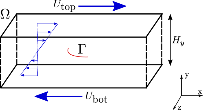
Fig. 1: Problem geometry for a single fiber $\Gamma$ located at the center of a periodic, rectangular channel $\Omega$ of dimension $H_{x}\times H_{y}\times H_{z}$. A planar shear flow is generated by forcing the top and bottom walls to move with constant velocities $\pm U_{top}$.

The fiber of length $L$ is placed at the center of the fluid domain which is specified by the constant $\boldsymbol{X}_{0}$, and we consider three different initial configurations for the fiber:

Configuration 1.

The fiber is initially straight and is parameterized by

$$\boldsymbol{X}(s,0) =\left((\epsilon_{0}+1)s,~{}0,~{}0\right)+\boldsymbol{X}_{0},$$

$$\boldsymbol{D}^{1}(s,0) =\left(0,~{}1,~{}0\right),$$

$$\boldsymbol{D}^{2}(s,0) =\left(0,~{}0,~{}1\right),$$

$$\boldsymbol{D}^{3}(s,0) =\left(1,~{}0,~{}0\right),$$

where $0\leq s<L$ and $\epsilon_{0}$ is a perturbation parameter that initially stretches the fiber.

Configuration 2.

The fiber is curved in the $xy$-plane with

$$\boldsymbol{X}(s,0) =\left(r_{0}\cos(s/r_{0}+\pi),~{}r_{0}\sin(s/r_{0}+\pi),~{}0\right)+\boldsymbol{X}_{0},$$

$$\boldsymbol{D}^{1}(s,0) =\left(0,~{}0,~{}1\right),$$

$$\boldsymbol{D}^{2}(s,0) =\left(\cos(s/r_{0}+\pi),~{}\sin(s/r_{0}+\pi),~{}0\right),$$

$$\boldsymbol{D}^{3}(s,0) =\left(\sin(s/r_{0}),~{}\cos(s/r_{0}+\pi),~{}0\right),$$

where $\alpha_{b}r_{0}\pi\leq s<\alpha_{e}r_{0}\pi$, and $\alpha_{b}$ and $\alpha_{e}$ are constants with $0\leq\alpha_{b}<\alpha_{e}\leq 1$. Here, the fiber is a segment of a circle of radius $r_{0}$ lying in the $xy$-plane and having length $L=(\alpha_{e}-\alpha_{b})\pi r_{0}$. Choosing a sufficiently large radius $r_{0}$ generates fiber with small initial curvature.

Configuration 3.

Similar to Configuration 2, except that the fiber is curved in the $xz$-plane with

$$\boldsymbol{X}(s,0) =\left((\epsilon_{0}+r_{0})\cos(s/r_{0}),~{}0,~{}(\epsilon_{0}+r_{0})\sin(s/r_{0})\right)+\boldsymbol{X}_{0},$$

$$\boldsymbol{D}^{1}(s,0) =\left(0,~{}-1,~{}0\right),$$

$$\boldsymbol{D}^{2}(s,0) =\left(\cos(s/r_{0}),~{}0,~{}\sin(s/r_{0})\right),$$

$$\boldsymbol{D}^{3}(s,0) =\left(\sin(s/r_{0}+\pi),~{}0,~{}\cos(s/r_{0})\right),$$

where $\alpha_{b}r_{0}\pi\leq s<\alpha_{e}r_{0}\pi$, and $\alpha_{b}$ and $\alpha_{e}$ are constants satisfying $0\leq\alpha_{b}<\alpha_{e}\leq 1$.

For all three configurations, the rod has open ends so that boundary conditions are required at $s=0$ and $L$. We assume that the internal force and moment vanish at the endpoints, corresponding to $\boldsymbol{F}^{\text{rod}}_{-1/2}=\boldsymbol{F}^{\text{rod}}_{N_{s}-1/2}=0$ and $\boldsymbol{N}^{\text{rod}}_{-1/2}=\boldsymbol{N}^{\text{rod}}_{N_{s}-1/2}=0$, which are consistent with the boundary conditions applied by Lim [27].

4 Numerical Method

Here, we provide only a very brief overview of the numerical method used to solve the governing equations, while a detailed description of the method and its parallel implementation can be found in [52, 53].

When discretizing the governing equations we use two separate computational grids, one each for the Eulerian and Lagrangian variables. The fluid domain is divided into an $N_{x}\times N_{y}\times N_{z}$, uniform, rectangular mesh where each cell has side length $h$. We employ a marker-and-cell (MAC) discretization [18] wherein the pressure is approximated at cell center points $\boldsymbol{x}_{i,j,k}$ for $i,j,k=0,1,\ldots,N-1$, while velocity components are located on cell faces. The Lagrangian variables are discretized at $N_{s}$ uniformly-spaced points denoted by $s_{\ell}=\ell\Delta s$ for $\ell=0,1,\ldots,N_{s}-1$ with $\Delta s=L/N_{s}$. Since our current implementation is restricted to periodic fluid domains, the top and bottom wall boundary conditions are imposed by slightly increasing the size of the fluid domain in the $y$-direction and introducing planes of IB tether points along $y=0$ and $H_{y}$ that are attached by very stiff springs to points moving at the specified velocities $U_{\text{top}}$ and $U_{\text{bot}}$. We did this for convience only, since neither the governing equations nor the fluid solver is restricted to periodic domains.

The IB equations are approximated using a fractional-step method described by Wiens and Stockie [53] in which the calculation of fluid variables is decoupled from that of the immersed boundary. For integrating the fluid equations, we use the pseudo-compressibility method developed by Guermond and Minev [15, 16], which employs a directional-splitting strategy that reduces to a series of one-dimensional tridiagonal systems. These linear systems can be solved efficiently on distributed-memory clusters by combining Thomas’s algorithm with a Schur-complement technique.

When integrating the rod position and orthonormal triad vectors forward in time, we use the predictor-corrector procedure devised by Griffith and Lim [12]. This differentiates our numerical method from the approach taken in [53], where an Adams–Bashforth extrapolation was used to evolve the immersed boundary in time. Although the predictor-corrector procedure introduces additional work, this change is necessary in order to obtain second-order convergence rates in space.

Lastly, the constitutive relations (9)–(14) are discretized in the same manner as in Lim et al. [28], with the main difference being in how the orthonormal triad vectors are interpolated onto half Lagrangian steps $s_{\ell+\frac{1}{2}}=(\ell+\frac{1}{2})\Delta s$. Here, we use the Rodrigues’ rotation formula as described in [52] instead of taking the principal square root used by Lim et al. [28].

If we assume that the state variables are all known at time $t_{n}$, the IB algorithm for a single time step $\Delta t$ proceeds as follows.

1. Interpolate the linear and angular fluid velocities onto the rod using the the delta kernel $\Phi_{w}(\boldsymbol{x})$ to obtain $\boldsymbol{U}^{n}$ and $\boldsymbol{W}^{n}$.

2. Predict the rod position $\boldsymbol{X}^{n+1,\ast}$ and orthonormal triad vectors $(\boldsymbol{D}^{\alpha})^{n+1,\ast}$ at time $t_{n+1}=(n+1)\Delta t$ to first order for $\alpha=1,2,3$.

3. Calculate the Lagrangian force and torque densities, $\boldsymbol{F}$ and $\boldsymbol{N}$, at times $t_{n}$ and $t_{n+1}$ using the discretization employed by Lim et al. [28].

4. Spread the Lagrangian force and torque densities just calculated onto fluid grid points. Then approximate the Eulerian force and torque density, $\boldsymbol{f}^{n+\frac{1}{2}}$ and $\boldsymbol{n}^{n+\frac{1}{2}}$, at time $t_{n+\frac{1}{2}}=(n+\frac{1}{2})\Delta t$ using an arithmetic average.

5. Integrate the incompressible Navier–Stokes equations to time $t_{n+1}$ using ($\boldsymbol{f}^{n+\frac{1}{2}}+\frac{1}{2}\nabla\times\boldsymbol{n}^{n+\frac{1}{2}}$) as the external body force.

6. Correct the rod position $\boldsymbol{X}^{n+1}$ and orthonormal triad $(\boldsymbol{D}^{\alpha})^{n+1}$ to second order. This requires interpolating the linear and angular fluid velocity at time $t_{n+1}$ onto the rod location.

5 Numerical Results

5.1 Intrinsically Straight Fibers

We begin by considering the behaviour of a single flexible fiber immersed in a shear flow, where the equilibrium fiber state is intrinsically straight (with no bend, no twist). As described earlier in Section 2, experimental observations show that such fibers are characterized by a well-defined orbital motion that can be separated into one of several distinct orbit classes according to a fiber flexibility parameter $\chi$ that captures the ratio of fiber bending force to hydrodynamic drag. This section aims to investigate the full range of these two-dimensional orbital motions.

In all simulations, we use the numerical parameters listed in Tables 2 and 3. Since the fiber motion is confined to the $xy$-plane, we significantly reduce the execution time of a simulation by shrinking the domain depth $H_{z}$, which allows us to run $100+$ simulations in a reasonable timeframe. Note that these results are virtually identical to simulations using a larger domain ($H_{z}=2$), which we confirmed through numerous computational experiments. In all simulations, we choose physical parameters that are consistent with natural (unbeaten) kraft pulp fibers, taking a fiber length of $0.1-0.3$ cm and flexural rigidity of $0.001-0.07\,\text{g cm}^{3}/\text{s}^{2}$ [8, 9]. Because fibers in our numerical simulations have diameter that is proportional to the effective thickness $w$, our simulated fibers are actually thicker than a natural pulp fiber. For example, we use a delta function regularization corresponding to $w\approx 80~{}\mu$m, whereas a natural pulp fiber has a diameter between $20$–$80~{}\mu$m. Since the precise dependence of the simulated fiber diameter on $w$ is unknown, we appeal to the work of Bringley and Peskin [4] where they observed that a one-dimensional array of rigid IB points has an effective numerical thickness of $D\approx 2w$. Although these results may not be strictly applicable in the present setting, this approximation is sufficient for our purposes. Any remaining discrepancy in the fiber diameter can then be accommodated for by adjusting the value of fiber drag force (see $F_{d}$ from equation (1)).

Table 2: Numerical and physical parameter values used in rigid fiber simulations.

Parameter	Symbol	Value
Size of fluid domain $\Omega$	$H_{x}\times H_{y}\times H_{z}$	$2\times\frac{1}{2}\times 16h$	cm
Number of fluid grid points	$N_{x}\times N_{y}\times N_{z}$	$256\times 64\times 16$
Fluid mesh width	$h$	$1/128$	cm
Fluid density	$\rho$	$1.0$	g/cm3
Fluid viscosity	$\mu$	$10.0$	g/(cm$\cdot$s)
Speed of moving plates	$U_{\text{top}}=U_{\text{bot}}$	$8$	cm/s
Shear rate	$G$	$32$	s-1
Time step	$\Delta t$	$1\text{e}{-5}$	s
Fiber length	$L$	$0.3$	cm
Fiber mesh width	$\Delta s$	$L/120$	cm
Bending and twisting modulus (EI)	$a_{1}=a_{2}=a_{3}$	$0.7$	$\text{dyne}\cdot\text{cm}^{2}$
Shear and stretch modulus	$b_{1}=b_{2}=b_{3}$	$540$	$\text{dyne}\cdot\text{cm}^{2}$
Fiber effective thickness	$w$	$0.0078125$	cm
Intrinsic twist vector	$\left(\kappa_{1},~{}\kappa_{2},~{}\tau\right)$	$\left(0,~{}0,~{}0\right)$
Fiber length perturbation	$\epsilon_{0}$	$0.001$
Support of delta kernel	$C$	$4$

In Figures 2 and 3, we display snapshots of the dynamics of a fiber with initial configuration lying in the $xy$-plane and for six values of the dimensionless flexibility parameter $\chi$ between $0.19$ and $1.125\text{e}{5}$. As expected, the simulations exhibit a range of different orbital motions that transition between the various orbit classes (rigid, springy, flexible, complex, coiled) as the flexibility increases. We also note that within the intermediate range of $\chi$ values, we observe both S turns and snake turns depending on the symmetry of the initial fiber configuration. Despite being very rare in actual fiber suspensions, S turns turn out to be remarkably stable in our idealized setting with a planar shear flow; indeed, it is only when asymmetry is introduced in the fiber through (for example) the initial shape or a length-dependent stiffness that snake turns are observed instead of S turns. These results are consistent with those of Mason and co-workers [1, 10] who observed that S turns required a high degree of symmetry that is rarely achieved in experiments. For the largest value of $\chi=1.125\text{e}{5}$ in Figure 33(c) we observe a coiled orbit with self-entanglement, and although this type of behaviour is not pertinent to pulp fibers, Forgacs and Mason [10] did observe such coiling with thread-like synthetic fibers. Eventually, this fiber forms a complex writhing bundle as the fiber undergoes self-contact, but because our model doesn’t incorporate any contact (fiber-on-fiber) forces we make no claim that these results correspond to physically accurate coiling dynamics.

Table 3: Parameter modifications for the flexible fiber simulations in Figures 2 and 3. Only those parameters that have changed relative to values indicated in Table 2 are shown here.

Orbit Class	Configuration	Parameters
Springy	2	$r_{0}=0.45$, $\alpha_{b}=0.4$, $\alpha_{e}=0.6$, $EI=2.5\text{e}{-2}$,
		$\Delta s\approx 1.25\text{e}{-3}$, $L\approx 0.282$
S turn	1	$EI=3.0\text{e}{-3}$
Snake turn	2	$r_{0}=0.45$, $\alpha_{b}=0.4$, $\alpha_{e}=0.6$, $EI=3.0\text{e}{-3}$,
		$\Delta s\approx 1.25\text{e}{-3}$, $L\approx 0.282$
Complex	2	$r_{0}=0.4$, $\alpha_{b}=0.4$, $\alpha_{e}=0.6$, $\mu=15$, $EI=1.0\text{e}{-3}$,
		$\Delta s\approx 1.25\text{e}{-3}$, $L\approx 0.251$
Coiled	1	$G=64,$ $\mu=90$, $EI=1.0\text{e}{-4}$, $L=0.5$

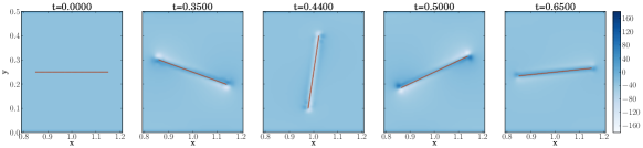
(a) Rigid Orbit ($\chi=0.19$, $EI=7.0\text{e}{-1}$, $L=0.3$)

(b) Springy Orbit ($\chi=4.49$, $EI=2.5\text{e}{-2}$, $L\approx 0.282$)

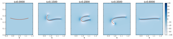
(c) Snake Orbit ($\chi=37.38$, $EI=3.0\text{e}{-3}$, $L\approx 0.282$)

Fig. 2: Snapshots of fiber position and fluid vorticity in the $xy$-plane for a half-rotation in a rigid, springy and snake orbit. Parameter values are listed in Tables 2 and 3.

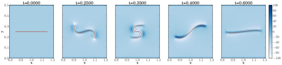
(a) S Orbit ($\chi=45.00$, $EI=3.0\text{e}{-3}$, $L=0.3$)

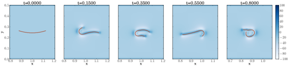
(b) Complex Orbit ($\chi=119.06$, $EI=1.0\text{e}{-3}$, and $L\approx 0.251$)

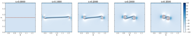
(c) Coiled Orbit ($\chi=1.125\text{e}{5}$, $EI=1.0\text{e}{-4}$, and $L=0.5$)

Fig. 3: Snapshots of fiber position and fluid vorticity in the $xy$-plane for an S turn, complex and coiled orbit. Parameter values are listed in Tables 2 and 3.

When the initial fiber configuration is rotated into the $xz$-plane, the resulting dynamics are non-planar but still follow orbits qualitatively similar to those derived by Jeffery [19]. Examples of these non-planar orbits are given in the first author’s doctoral thesis [52], which show that the flexible fiber undergoes a motion consisting of a rotations in the $xy$-plane superimposed on a rocking motion back and forth about the $z$-axis in the $xz$-plane.

We next explore in more detail the dependence of the fiber orbit class on the dimensionless flexibility parameter $\chi$. To this end, we perform a much larger series of simulations with varying fiber length ($L=0.1$–$0.3$ cm), diameter ($D\approx 156$–$312~{}\mu$m), flexural rigidity ($EI=0.001$–$0.1~{}\text{dyne}\cdot\text{cm}^{2}$), shear rate ($G=20$–$120$ s^-1) and viscosity ($\mu=0.07$–$100.0$ g/(cm$\cdot$s)) corresponding to Reynolds numbers lying in the range $0.0027$–$23.9$. For each simulation, we assign the fiber dynamics to one of the four orbit classes I–IV by calculating the total fiber curvature

$$\lambda(t)=\int_{0}^{L}\left|\frac{\partial\boldsymbol{D}^{3}}{\partial s}(s,t)\right|\,ds,$$

and using the maximum curvature over a half-rotation $t_{0}\leq t\leq t_{1}$ to apply the following criteria:

• I: The orbit is rigid if $\displaystyle\max_{t_{0}\leq t\leq t_{1}}\lambda(t)<0.4$.

• II: The orbit is springy if $\displaystyle 0.4\leq\max_{t_{0}\leq t\leq t_{1}}\lambda(t)<3.7$.

• III: The orbit is an S or snake turn if $\displaystyle 3.7\leq\max_{t_{0}\leq t\leq t_{1}}\lambda(t)$ and $\lambda(t_{1})<2.5$.

• IV: The orbit is complex if $\displaystyle 3.7\leq\max_{t_{0}\leq t\leq t_{1}}\lambda(t)$ and $\displaystyle 2.5\geq\lambda(t_{1})$.

Note that S/snake turns and complex rotations have the same range of maximum curvature, and that we use the fiber curvature $\lambda(t_{1})$ at the end of the half-rotation to determine whether or not the fiber has straightened out.

Simulations are depicted graphically in Figure 4 in terms of two plots of flexural rigidity $EI$ and drag force $F_{d}$ versus dimensionless flexibility $\chi$. Each point on the plot corresponds to a simulation using a specific choice of physical parameters, and the point type is assigned based on the orbit classification criteria above. From these two plots, it is evident that there is a clear division of orbits into classes I, II and III along vertical divisions that correspond to values of $\chi\cong 3.85$ and $\chi\cong 20.0$. The boundary between classes III and IV is not as sharply defined, but can still be assigned to a value of flexibility $\chi\approx 65.0$. Based on these observations, we conclude that the dimensionless flexibility $\chi$ provides a useful measure for characterizing orbit classes at the lower Reynolds numbers considered here.

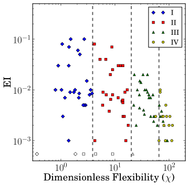
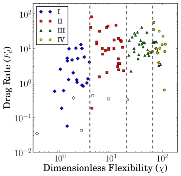
Fig. 4: Summary of all simulations showing the relationship between orbit class and different values of the dimensionless flexibility $\chi$, flexural rigidity $EI$ and drag rate $F_{d}$. Open markers denote the experimental data shown in Table 4 where $E=3$ GPa.

We conclude this section by performing a further comparison of our numerical simulations with the experiments of Forgacs and Mason [10] on dacron fibers in corn syrup. First of all, we list the parameters and observed orbit class for several of these experiments in Table 4. Based on values of $\chi\cdot EI$, we see that this rescaled flexibility parameter may be used to classify each orbit, assuming that $EI$ is constant in all experiments. However, we emphasize that since Forgacs and Mason did not provide a value for the flexural rigidity ($EI$), we were unable to determine the value of $\chi$ explicitly.

Table 4: Experimental results obtained from Forgacs and Mason [10] for synthetic dacron fibers.

Orbit Class	$\chi\cdot EI$	$G$ (s-1)	$\mu$ (g/(cm$\cdot$s))	$L$ (cm)	$D$ ($\mu$m)
Rigid	$1.96\text{e}{-4}$	$3.921$	$11.4$	$0.1778$	$7.8$
Rigid	$1.01\text{e}{-3}$	$5.143$	$91.2$	$0.1404$	$7.8$
Springy	$1.43\text{e}{-3}$	$4.763$	$11.4$	$0.3229$	$7.8$
Springy	$2.39\text{e}{-3}$	$5.965$	$91.2$	$0.1778$	$7.8$
Springy	$4.91\text{e}{-3}$	$4.879$	$91.2$	$0.2418$	$7.8$
Flexible	$1.16\text{e}{-2}$	$4.825$	$91.2$	$0.3229$	$7.8$

Because these experiments were all performed with dacron fibers, we next explore further the assumption that $EI$ is roughly constant, and also whether the experimental results are consistent with the division of orbit classes in our simulations in Figure 4. First of all, we remark that all experimental data points are consistent with our simulations if $2.46\text{e}{-4}<EI<3.71\text{e}{-4}$ ($\text{dyne}\cdot\text{cm}^{2}$).  Unfortunately, the Young’s modulus $E$ for dacron is known to vary over an extremely wide range of $71.5\text{ MPa}\leq E\leq 22.1\text{ GPa}$ between various manufacturers [6]. However, the manufacturer of the fibers used by Forgacs and Mason was identified as E.I. du Pont de Nemours and Co., and we were able to find a patent filed by this company in 1969 [5] for several dacron blends that lists a much tighter range for Young’s modulus of $2.0\text{ GPa}<E<3.5\text{ GPa}$. Therefore, the hypothetical $EI$ of these synthetic fibers would be between $3.63\text{e}{-4}<EI<6.36\text{e}{-4}$, which is consistent with our numerical results! Furthermore, most data points are still classified correctly when the $EI$ falls outside our consistency range ($2.46\text{e}{-4}<EI<3.71\text{e}{-4}$). To illustrate, we have plotted the experimental data in Figure 4 using open markers, assuming $E=3$ GPa (giving an $EI=5.45\text{e}{-4}$). Here, we observe that all experimental data are classified correctly, except for one troublesome data point. Therefore, we conclude from these results that our simulations are in excellent agreement with experimental data.

5.2 Intrinsically Curved Fibers

We next consider single flexible fibers that have an intrinsic curvature at equilibrium, a situation that is often encountered for natural fibers such as wood pulp. We use the base parameter values in Table 2 and simulate two cases corresponding to the modifications listed in Table 5. In both cases, the fiber is initialized as a curved segment of a circular arc with intrinsic twist vector $\left(\kappa_{1},~{}\kappa_{2},~{}\tau\right)=\left(1/r_{0},~{}0,~{}0\right)$, which keeps the initial fiber configuration at equilibrium (that is, $N^{1}=N^{2}=N^{3}=0$ at $t=0$).

Table 5: Parameter modifications for the flexible fiber simulations in Figure 5 and 6. Only those parameters that have changed relative to values in Table 2 are shown here.

Orbit Class	Configuration	Parameters
S turn	3	$H_{z}=2$, $r_{0}=0.45$, $\alpha_{b}=0.4$, $\alpha_{e}=0.6$, $EI=3.0\text{e}{-3}$,
		$\epsilon_{0}=1\text{e}{-3}$, $\Delta s\approx 1.25\text{e}{-3}$, $L\approx 0.282$
Snake turn	2	$H_{z}=2$, $r_{0}=0.45$, $\alpha_{b}=0.4$, $\alpha_{e}=0.6$, $EI=3.0\text{e}{-3}$,
		$\Theta_{xz}=\pi/16$, $\Delta s\approx 1.25\text{e}{-3}$, $L\approx 0.282$

The resulting orbits depicted in Figures 5 and 6 clearly correspond to S- and snake-like orbits. The projections of both fibers in the $xy$-plane behave like the corresponding planar orbits considered in Section 5.1, but protrude into the $xz$-plane. These simulations reproduce similar orbital dynamics to those observed in experiments of Arlov et al. [1]. The first author’s thesis [52] shows additional simulations for a fiber initially oriented along the $z$-direction and undergoing an additional axial spin, for which the fiber rotates around the $z$-axis and slightly straightens out as it rotates into the shear flow.

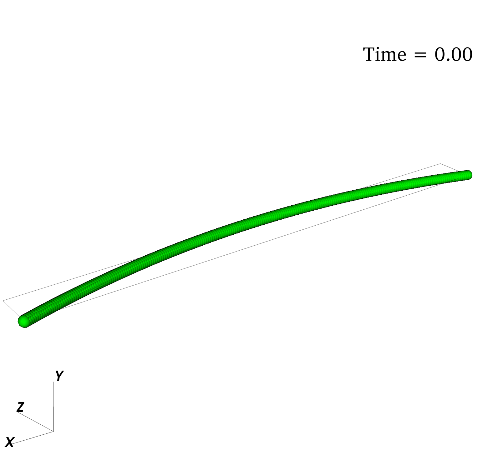
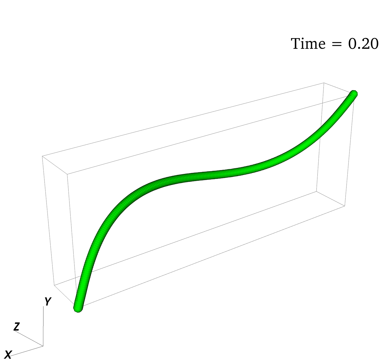
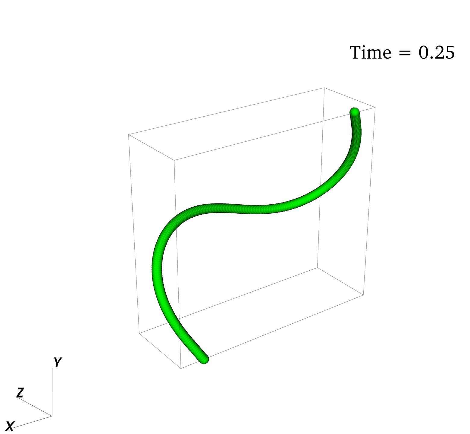
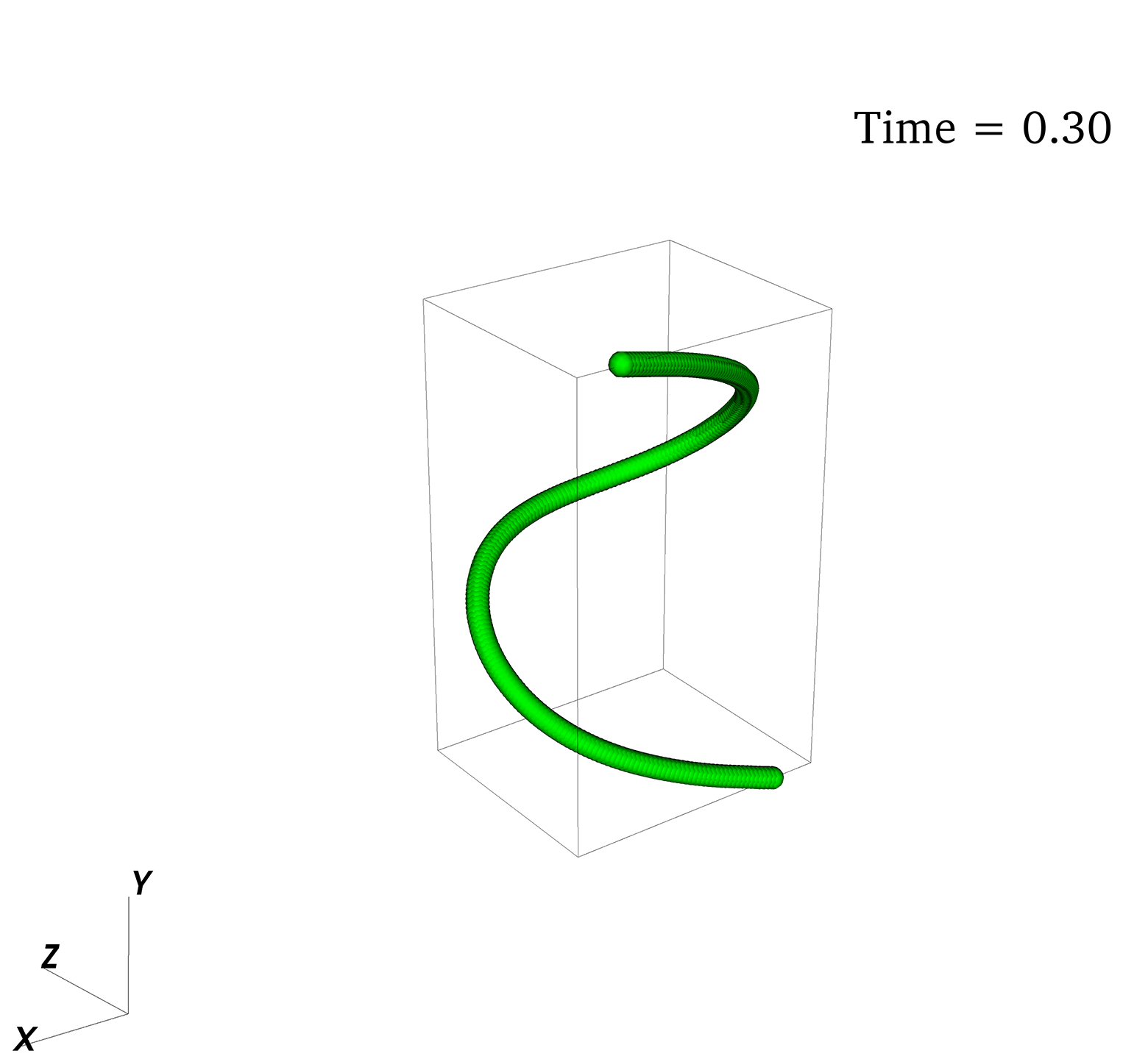
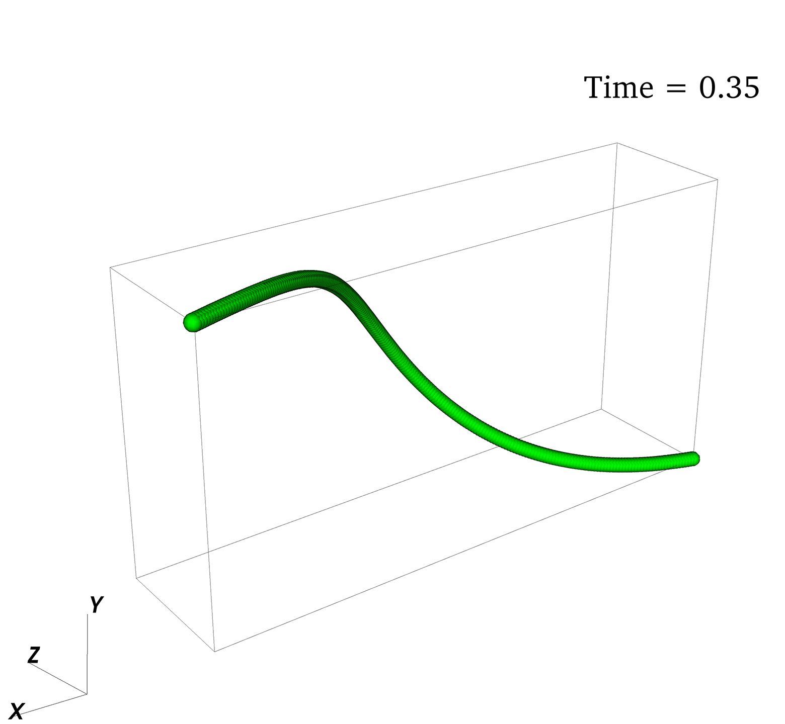
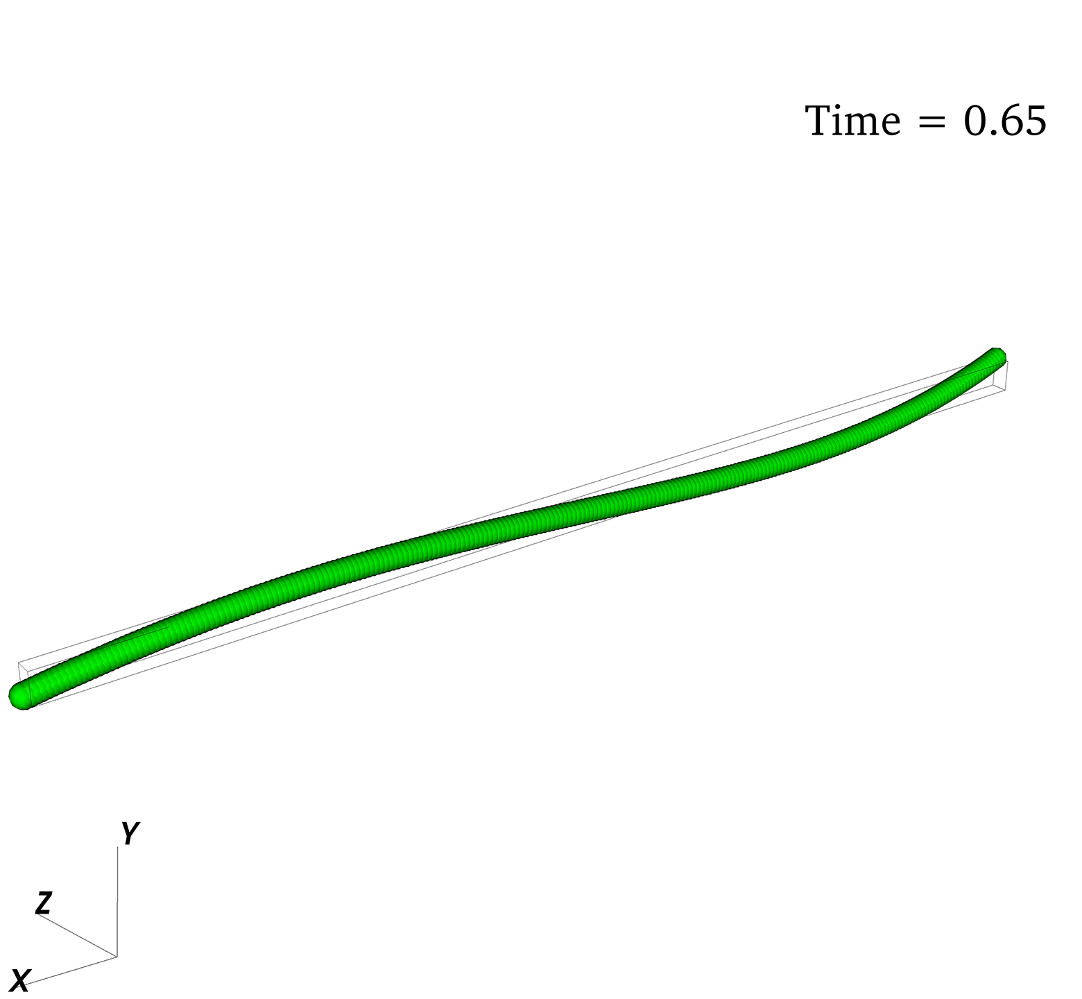
Fig. 5: Snapshots of an S turn orbit for an intrinsically curved fiber with parameters in Tables 2 and 5.

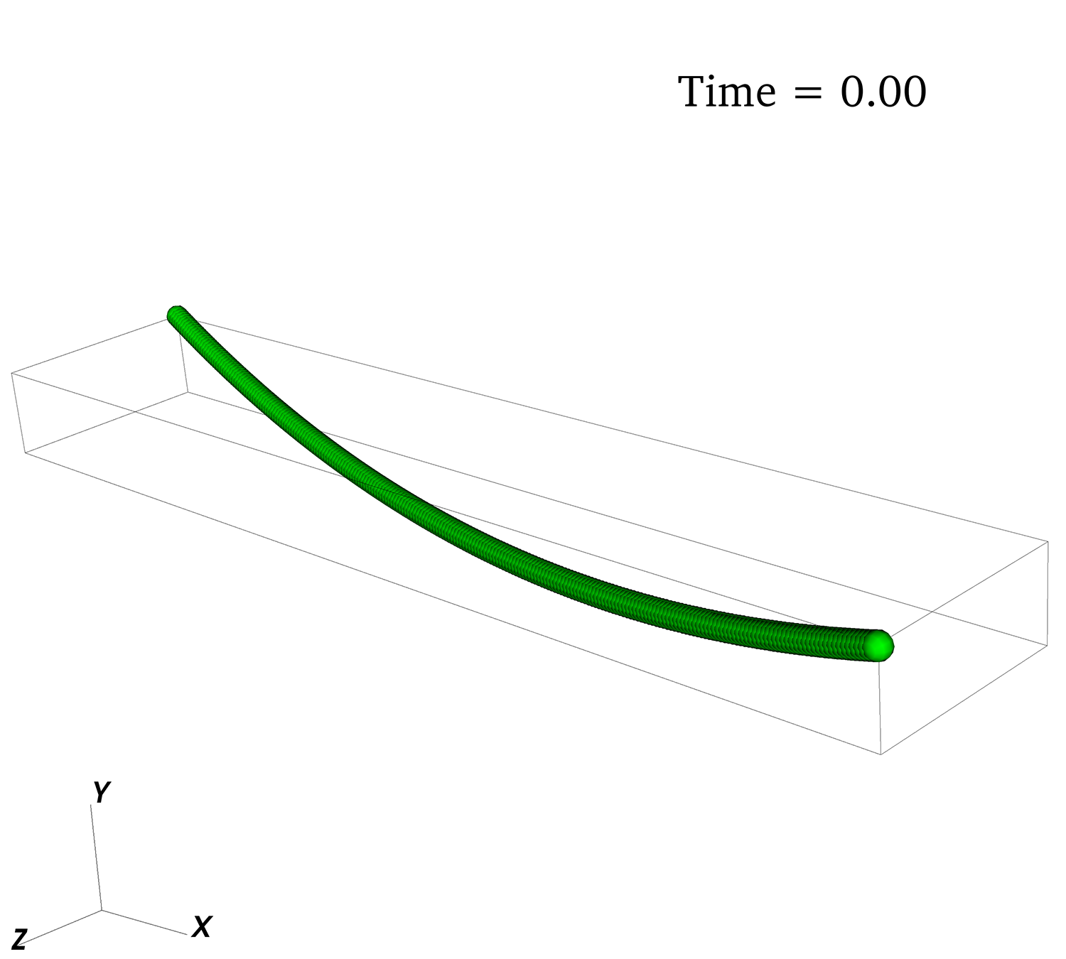
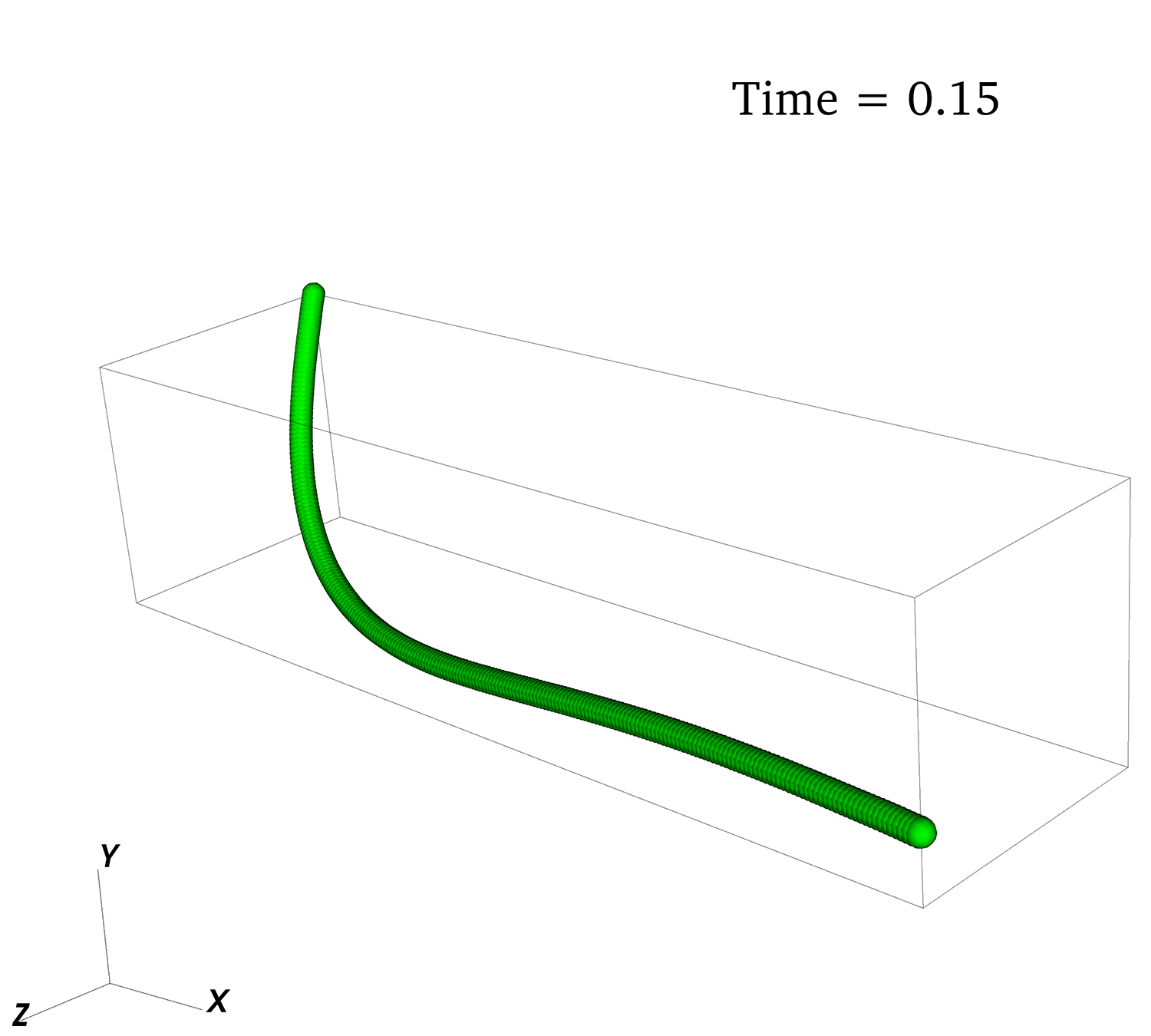
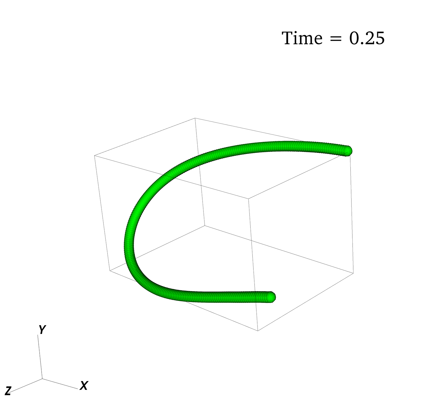
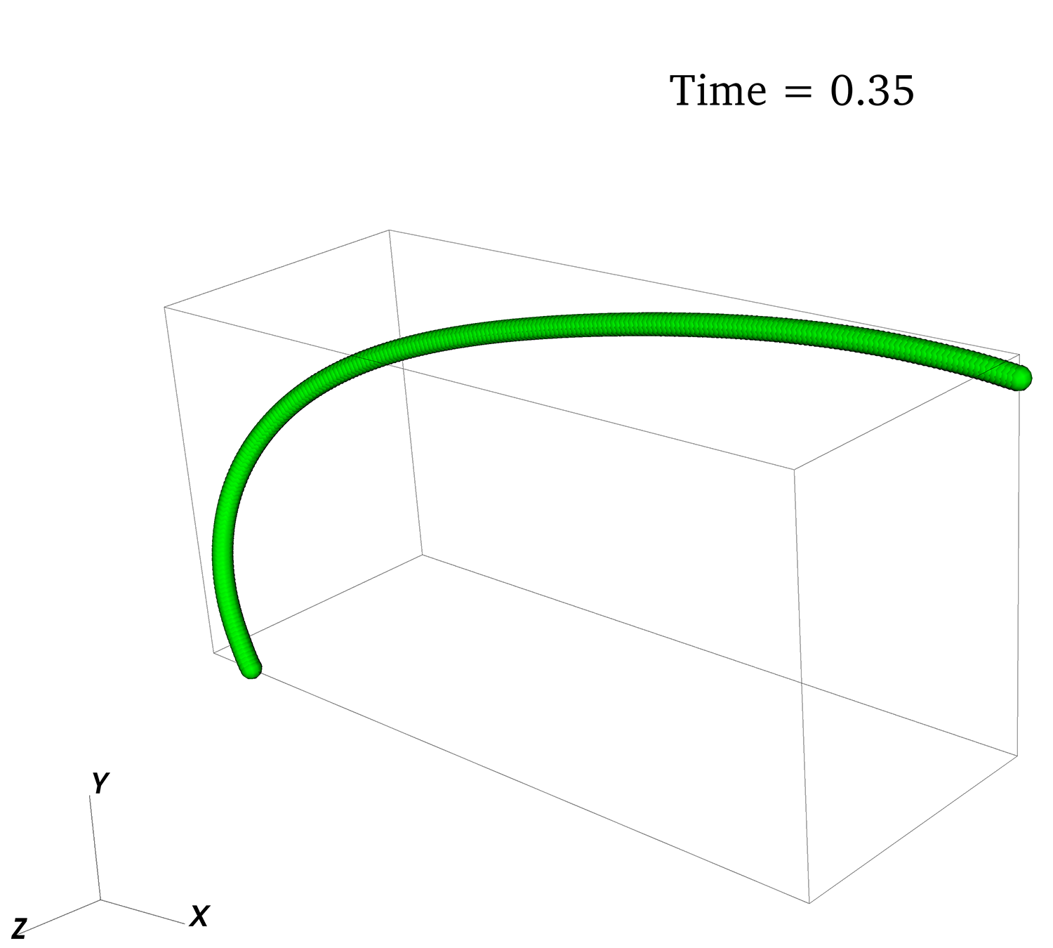
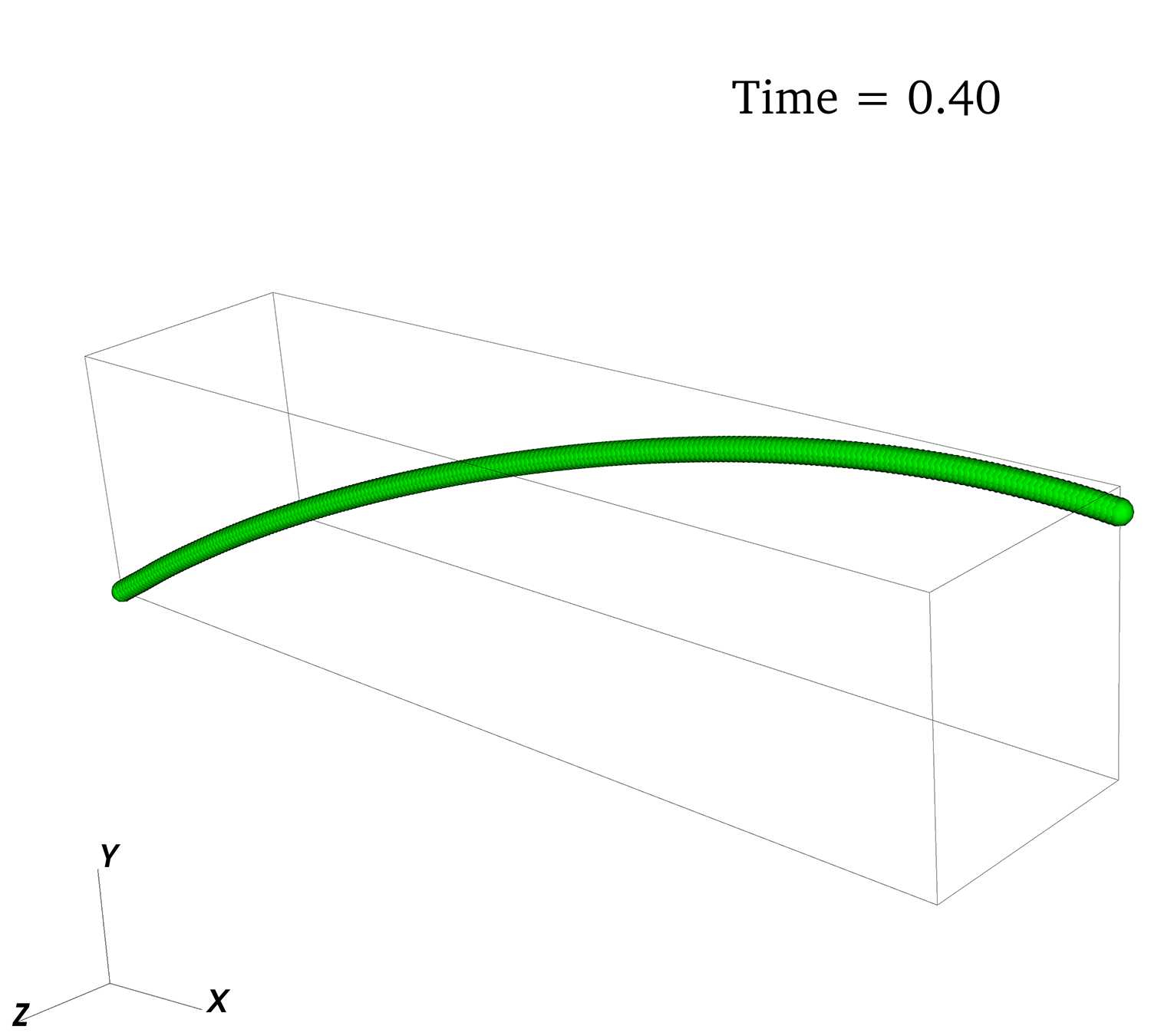
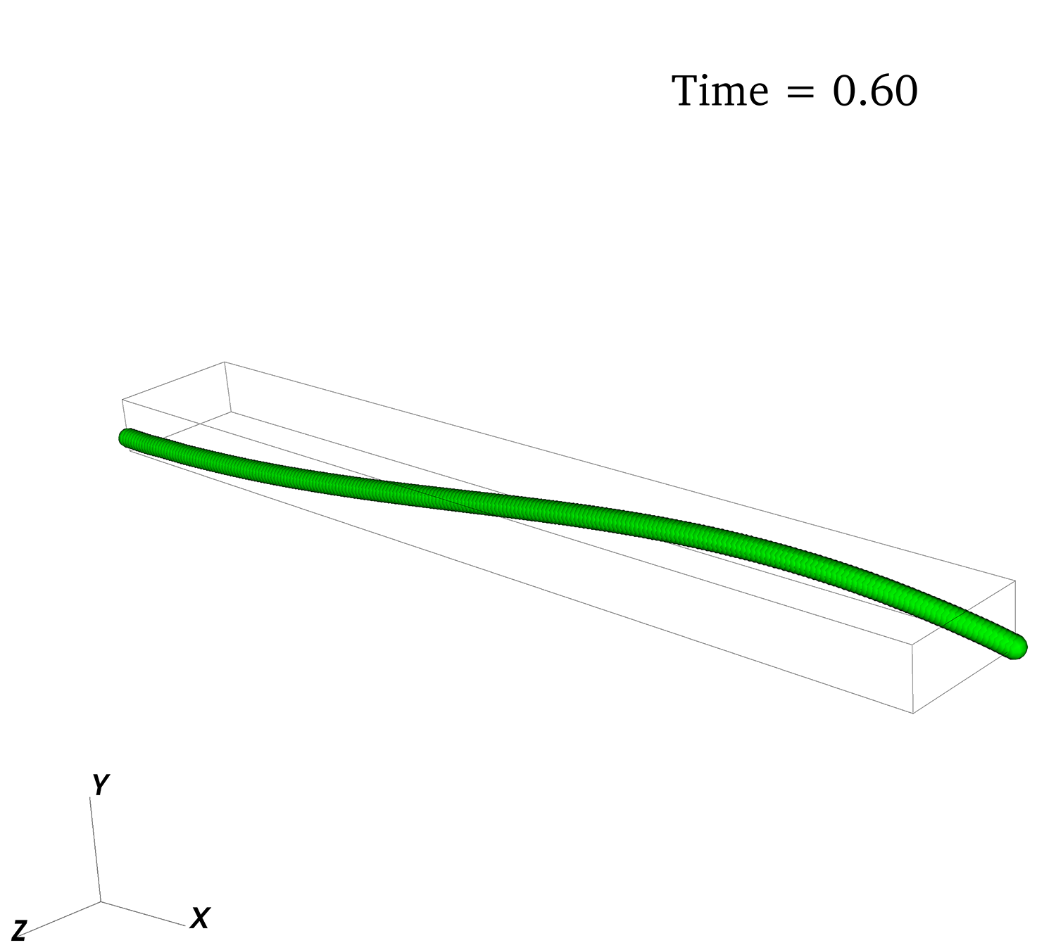
Fig. 6: Snapshots of snake turn for an intrinsically curved fiber with parameters in Tables 2 and 5.

5.3 Multiple Flexible Fibers

For our last series of simulations, we consider an idealized representation of a fiber suspension that permits us to employ the domain tiling techniques described in [53]. In these computations, we simulate a $P_{x}\times 1\times P_{z}$ array of fibers immersed in the fluid domain $\Omega=[0,P_{x}H_{x}]\times[0,H_{y}]\times[0,P_{z}H_{z}]$ using the boundary conditions stated in Section 3.1. The code runs in parallel on a $P=P_{x}\times P_{z}$ array of computer processors ($P_{y}=1$) and the fluid domain $\Omega$ is partitioned along the $x$- and $z$-axes so that one processor labelled $I,K$ is responsible for each subdomain $\Omega_{I,K}=[(I-1)H_{x},IH_{x}]\times[0,H_{y}]\times[(K-1)H_{z},KH_{z}]$, for $I=1,2,\ldots,P_{x}$ and $K=1,2,\ldots P_{z}$. We have constructed this problem so that it can be used as a weak scalability test, wherein the local problem size is held fixed as both the number of processors and global problem size are increased. It is important to recognize that our method is in no way restricted to such idealized arrays of fibers, but rather we have employed this arrangement here in order to clearly illustrate the parallel scalability of our algorithm.

Initially, each subdomain $\Omega_{I,K}$ contains a single intrinsically-curved fiber located at its centroid, with a randomly-chosen orientation angle and whose initial shape is defined in the same manner as described earlier for Configuration 3. The numerical and physical parameters are as in Table 2 with the following modifications: $H_{x}=0.421875$, $H_{y}=\frac{1}{2}$, $H_{z}=0.3125$, $\Delta t=5\text{e}{-5}$, $r_{0}=0.45$, $\alpha_{b}=0.4$, $\alpha_{e}=0.6$, $EI=3.0\text{e}{-3}$, $\Delta s\approx 1.25\text{e}{-3}$, $L\approx 0.282$, $U_{\text{top}}=8.5$ and $U_{\text{bot}}=7.5$. Another difference from our earlier simulations is that the top and bottom boundaries that induce the shear flow now move at different speeds (that is, $U_{\text{top}}\neq U_{\text{bot}}$); consequently, fibers are transported across subdomain boundaries which provides a nontrivial test of our algorithm’s ability to handle inter-process communication as well as changes to the IB data stored on each processor over time.

Figure 7 presents three snapshots of the dynamics of a $16\times 16$ array of fibers at the initial and two later times. The image at time $t=0.25$ emphasizes the fact that all fibers spend the majority of their time aligned horizontally with the shear flow (i.e., along the $x$-axis) and that only a small proportion of the fibers at any time instant are rotated out of the shear plane. As the suspension evolves over time, the fibers are prone to drift and cluster together, leading to development of more complex behavior such as is shown in the image at time $t=1.80$. This last snapshot suggests that our algorithm is capable of simulating at least the initial phases fiber flocculation in a suspension with a reasonable concentration of fibers.

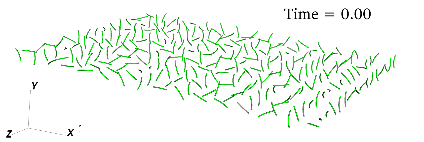
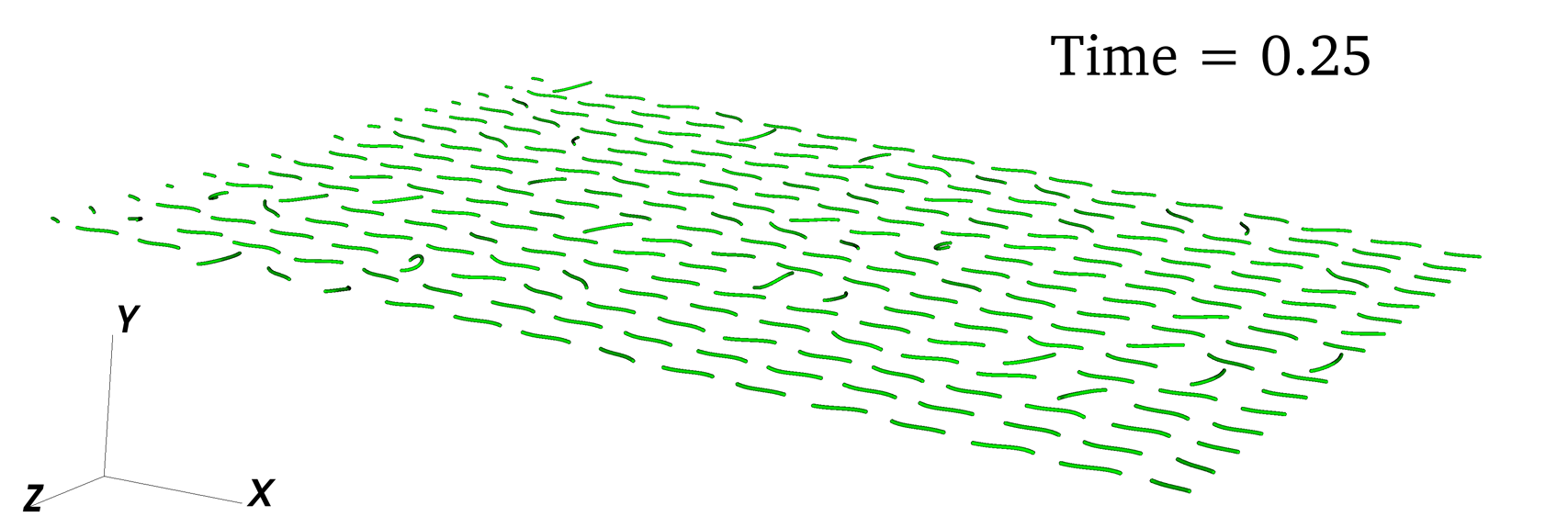
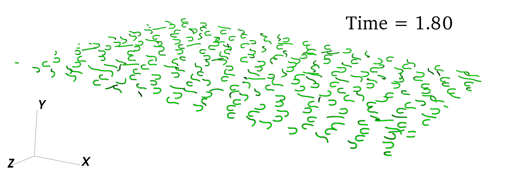
Fig. 7: A suspension of $256$ intrinsically-curved fibers ($P_{x}=P_{z}=16$) in Configuration $3$. Parameters are described in Section 5.3.

The next set of results attempts to quantify the importance of including the full two-way fluid-structure interaction between fluid and fibers, relative to other more common numerical approaches that simplify or eliminate this interaction. For this purpose, we define a quantity we call the local deviation as

$${\mathcal{E}}_{\text{rel}}(\boldsymbol{x},t)=\frac{|\boldsymbol{u}(\boldsymbol{x},t)-\boldsymbol{u}(\boldsymbol{x},0)|}{\max_{\boldsymbol{x}}(|\boldsymbol{u}(\boldsymbol{x},0)|)},$$

which is a local measure of the relative difference between the computed fluid velocity and the corresponding linear shear flow that would arise in the absence of any fibers. We also define a related global deviation from linear shear using either the $\ell^{\infty}$-norm

$$\|{\mathcal{E}}_{\text{rel}}(\boldsymbol{x},t)\|_{\infty}=\max_{i,j,k}|{\mathcal{E}}_{\text{rel}}(\boldsymbol{x}_{i,j,k},t_{n})|,$$

or $\ell^{1}$-norm

$$\|{\mathcal{E}}_{\text{rel}}(\boldsymbol{x},t)\|_{1}=\frac{h^{3}}{V}\sum_{i,j,k}|{\mathcal{E}}_{\text{rel}}(\boldsymbol{x}_{i,j,k},t_{n})|,$$

where $V$ is the fluid volume. For a 25-fiber simulation computed with $(P_{x},P_{y},P_{z})=(5,1,5)$ processors, we provide plots in Figure 8 of the local deviation ${\mathcal{E}}_{\text{rel}}$ at time $t=1.80$ and along two different horizontal slices. The figures have truncated the values of ${\mathcal{E}}_{\text{rel}}$ above the threshold 0.025 so that smaller deviations can be visualized. From these plots we observe that the local deviation is largest adjacent to the individual fibers where the no-slip condition forces the fluid to follow the deforming and rotating fibers, but that the deviation decays rapidly away from the fibers. Nonetheless, there are still significant fluid disturbances spread throughout the entire fluid domain that influence fiber motion and are related to hydrodynamic interactions between individual fibers. The corresponding global deviation values are $\|{\mathcal{E}}_{\text{rel}}\|_{1}=0.0159$ and $\|{\mathcal{E}}_{\text{rel}}\|_{\infty}=0.135$ which show that relative deviations in the flow are as high as 13.5% near the fibers but that the average over the entire flow field is only about 1.6%. Other simulations using different parameters and initial conditions yield similar results (see [52]) with the average relative deviation hovering around 2% and the maximum ranging up to 40%. These results suggest that incorporating the full fluid-structure interaction into models for non-dilute suspensions is important in terms of properly capturing the dynamics of the flexible fibers. We also note that these simulations are performed at relative low values of Reynolds number and fiber concentration, and that the deviation measure will only get larger as the Reynolds number and concentration increase.

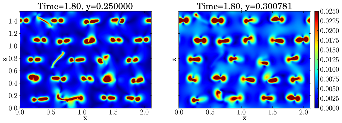
Fig. 8: Fluid deviation ${\mathcal{E}}_{\text{rel}}$ on two horizontal planes for the $25$ fiber simulation computed in Table 6. Plotted values are truncated at the threshold ${\mathcal{E}}_{\text{rel}}=0.025$.

Finally, we close by investigating the parallel performance of our IB algorithm by considering simulations of different-sized suspensions of fibers on multiple processors. Based on our problem setup, the execution time would ideally stay constant as the global problem size and number of processors increase. Indeed, Table 6 shows that as the size of the fiber array ($P_{x}$, $P_{z}$) is increased, there is only a slight increase in execution time and hence our algorithm is said to be weakly scalable. We remark that our code is still not fully optimized and that the algorithm performance could be further improved by making enhancements such as enforcing the top/bottom wall boundary conditions directly instead of our approach of treating the walls using IB tether points.

Table 6: Weak scaling results showing the average execution time per time step (in seconds) for the multiple fiber problem. The local problem size is held fixed as the number of processors $P$ (and global problem size) is increased. Simulations are run on the Bugaboo cluster managed by WestGrid [49].

$P$	($P_{x},P_{y},P_{z}$)	Wall Time
$25$	($5,1,5$)	$0.57$
$64$	($8,1,8$)	$0.58$
$144$	($12,1,12$)	$0.58$
$225$	($15,1,15$)	$0.62$
$256$	($16,1,16$)	$0.61$

6 Conclusions

In this paper, we have presented a parallel immersed boundary algorithm for simulating suspensions of flexible fibers, where individual fibers are modelled as Kirchhoff rods. The novelty of this work derives from its application to multi-fiber suspension flows with non-zero Reynolds number and the inclusion of the the full two-way interaction between the fluid and suspended fibers. In our numerical simulations, we reproduce the full range of orbital dynamics observed experimentally by Mason and co-workers for isolated fibers immersed in a linear shear flow. When extending the results to multi-fiber suspensions, we demonstrate through a weak scalability test that the parallel scaling of our algorithm is near optimal and hence shows promise for simulating more complex scenarios such as semi-dilute suspensions and fiber flocculation.

In the future, we plan to improve on the underlying model, which will allow us to simulate more realistic fiber suspensions. First, we plan on incorporating the contact forces between fibers such as the frictional forces modelled by Schmid et al. [40]. Second, we will incorporate the effect of added fiber mass using the penalty IB method [22]. After incorporating these extensions, a more extensive comparison to experimental data would be required, comparing quantities such as the specific viscosity of the suspension [37].

References

- [1] A. P. Arlov, O. L. Forgacs, and S. G. Mason. Particle motions in sheared suspensions IV. General behaviour of wood pulp fibres. svenskpapp, 61(3):61–67, 1958.
- [2] G. K. Batchelor. Slender-body theory for particles of arbitrary cross-section in Stokes flow. Journal of Fluid Mechanics, 44(3):419–440, 1970.
- [3] F. P. Bretherton. The motion of rigid particles in a shear flow at low Reynolds number. Journal of Fluid Mechanics, 14(2):284–304, 1962.
- [4] T. T. Bringley and C. S. Peskin. Validation of a simple method for representing spheres and slender bodies in an immersed boundary method for Stokes flow on an unbounded domain. Journal of Computational Physics, 227:5397–5425, 2008.
- [5] O. Cope. Polymer blends of polyethylene terephthalate and alpha-olefin,alpha,beta-unsaturated carboxylic acid copolymers, March 25 1969. US Patent 3,435,093.
- [6] Dacron flexural modulus. WolframAlpha. Retrieved February 10, 2014 from \urlhttp://www.wolframalpha.com/input/?i=dacron+flexural+modulus.
- [7] E. H. Dill. Kirchhoff’s theory of rods. Archive for History of Exact Sciences, 44(1):1–23, 1992.
- [8] P. A. T. Doo and R. J. Kerekes. A method to measure wet fiber flexibility. Tappi Journal, 64(3):113–116, 1981.
- [9] P. A. T. Doo and R. J. Kerekes. The flexibility of wet pulp fibres. Pulp and Paper Canada, 83(2):46–50, 1982.
- [10] O. L. Forgacs and S. G. Mason. Particle motions in sheared suspensions X. orbits of flexible threadlike particles. Journal of Colloid Science, 14:473–491, 1959.
- [11] O. L. Forgacs, A. A. Robertson, and S. G. Mason. The hydrodynamic behaviour of paper-making fibres. Pulp Paper Magazine, 59(5):117–128, 1958.
- [12] B. E. Griffith and S. Lim. Simulating an elastic ring with bend and twist by an adaptive generalized immersed boundary method. Communications in Computational Physics, 12(2):433, 2012.
- [13] B. E. Griffith, X. Y. Luo, D. M. McQueen, and C. S. Peskin. Simulating the fluid dynamics of natural and prosthetic heart valves using the immersed boundary method. International Journal of Applied Mechanics, 1(1):137–177, 2009.
- [14] B. E. Griffith and C. S. Peskin. On the order of accuracy of the immersed boundary method: Higher order convergence rates for sufficiently smooth problems. Journal of Computational Physics, 208(1):75–105, 2005.
- [15] J. L. Guermond and P. D. Minev. A new class of fractional step techniques for the incompressible Navier-Stokes equations using direction splitting. Comptes Rendus Mathematique, 348:581–585, 2010.
- [16] J. L. Guermond and P. D. Minev. A new class of massively parallel direction splitting for the incompressible Navier-Stokes equations. Computer Methods in Applied Mechanics and Engineering, 200(23-24):2083–2093, 2011.
- [17] C. Hamlet, A. Santhanakrishnan, and L. A. Miller. A numerical study of the effects of bell pulsation dynamics and oral arms on the exchange currents generated by the upside-down jellyfish Cassiopea xamachana. Journal of Experimental Biology, 214:1911–1921, 2011.
- [18] F. H. Harlow and J. E. Welch. Numerical calculation of time-dependent viscous incompressible flow of fluid with free surface. Physics of Fluids, 8(12):2182–2189, 1965.
- [19] G. B. Jeffery. The motion of ellipsoidal particles immersed in a viscous fluid. Proceedings of the Royal Society of London. Series A, 102(715):161–179, 1922.
- [20] C. G. Joung, N. Phan-Thien, and X. J. Fan. Direct simulation of flexible fibers. Journal of Non-Newtonian Fluid Mechanics, 99(1):1–36, 2001.
- [21] M. Keshtkar, M. C. Heuzey, and P. J. Carreau. Rheological behavior of fiber-filled model suspensions: Effect of fiber flexibility. Journal of Rheology, 53(3):631–650, 2009.
- [22] Y. Kim and C. S. Peskin. Penalty immersed boundary method for an elastic boundary with mass. Physics of Fluids, 19(5):053103, 2007.
- [23] Y. Kim and C. S. Peskin. 3D parachute simulation by the immersed boundary method. Computers & Fluids, 38(6):1080–1090, 2009.
- [24] Y. Kim, Y. Seol, M. C. Lai, and C. S. Peskin. The immersed boundary method for two-dimensional foam with topological changes. Communications in Computational Physics, 12(2):479, 2012.
- [25] M. C. Lai and C. S. Peskin. An immersed boundary method with formal second-order accuracy and reduced numerical viscosity. Journal of Computational Physics, 160(2):705–719, 2000.
- [26] L. Li, H. Manikantan, D. Saintillan, and S. E. Spagnolie. The sedimentation of flexible filaments. Journal of Fluid Mechanics, 735:705–736, 2013.
- [27] S. Lim. Dynamics of an open elastic rod with intrinsic curvature and twist in a viscous fluid. Physics of Fluids, 22(2):024104–024104, 2010.
- [28] S. Lim, A. Ferent, X. S. Wang, and C. S. Peskin. Dynamics of a closed rod with twist and bend in fluid. SIAM Journal on Scientific Computing, 31(1):273–302, 2008.
- [29] S. B. Lindström and T. Uesaka. Simulation of the motion of flexible fibers in viscous fluid flow. Physics of Fluids, 19(11):113307, 2007.
- [30] S. B. Lindström and T. Uesaka. Simulation of semidilute suspensions of non-brownian fibers in shear flow. Journal of Chemical Physics, 128(2):024901, 2008.
- [31] S. B. Lindström and T. Uesaka. A numerical investigation of the rheology of sheared fiber suspensions. Physics of Fluids, 21:083301, 2009.
- [32] Y. Mori and C. S. Peskin. Implicit second-order immersed boundary methods with boundary mass. Computer Methods in Applied Mechanics and Engineering, 197(25–28):2049–2067, 2008.
- [33] H. Nguyen and L. Fauci. Hydrodynamics of diatom chains and semiflexible fibres. Journal of The Royal Society Interface, 11(96):20140314, 2014.
- [34] S. D. Olson, S. Lim, and R. Cortez. Modeling the dynamics of an elastic rod with intrinsic curvature and twist using a regularized Stokes formulation. Journal of Computational Physics, 2013.
- [35] C. S. Peskin. Flow Patterns Around Heart Valves: A Numerical Method. Journal of Computational Physics, 10:252–271, 1972.
- [36] C. S. Peskin. The immersed boundary method. Acta Numerica, 11:479–517, 2002.
- [37] C. J. S. Petrie. The rheology of fibre suspensions. Journal of Non-Newtonian Fluid Mechanics, 87(2):369–402, 1999.
- [38] K. A. Rejniak and R. H. Dillon. A single cell-based model of the ductal tumour microarchitecture. Computational and Mathematical Methods in Medicine, 8(1):51–69, 2007.
- [39] R. F. Ross and D. J. Klingenberg. Dynamic simulation of flexible fibers composed of linked rigid bodies. Journal of Chemical Physics, 106:2949–2960, 1997.
- [40] C. F. Schmid, L. H. Switzer, and D. J. Klingenberg. Simulations of fiber flocculation: Effects of fiber properties and interfiber friction. Journal of Rheology, 44(3):781–809, 2000.
- [41] P. Skjetne, R. F. Ross, and D. J. Klingenberg. Simulation of single fiber dynamics. Journal of Chemical Physics, 107:2108–2121, 1997.
- [42] J. M. Stockie. Analysis and Computation of Immersed Boundaries, with Application to Pulp Fibres. PhD thesis, Institute of Applied Mathematics, University of British Columbia, Vancouver, Canada, 1997. Available from \urlhttps://circle.ubc.ca/handle/2429/7346.
- [43] J. M. Stockie. Simulating the dynamics of flexible wood pulp fibres in suspension. In Proceedings of the 16th Annual International Symposium on High Performance Computing Systems and Applications, page 154. IEEE Computer Society, 2002.
- [44] J. M. Stockie and S. I. Green. Simulating the motion of flexible pulp fibres using the immersed boundary method. Journal of Computational Physics, 147(1):147–165, 1998.
- [45] L. H. Switzer and D. J. Klingenberg. Flocculation in simulations of sheared fiber suspensions. International Journal of Multiphase Flow, 30(1):67–87, 2004.
- [46] L. H. Switzer III and D. J. Klingenberg. Rheology of sheared flexible fiber suspensions via fiber-level simulations. Journal of Rheology, 47(3):759–778, 2003.
- [47] A. K. Tornberg and M. J. Shelley. Simulating the dynamics and interactions of flexible fibers in Stokes flows. Journal of Computational Physics, 196:8–40, 2004.
- [48] G. Wang, W. Yu, and C. Zhou. Optimization of the rod chain model to simulate the motions of a long flexible fiber in simple shear flows. European Journal of Mechanics-B/Fluids, 25(3):337–347, 2006.
- [49] WestGrid. QuickStart Guide to Bugaboo. Retrieved April 11, 2013 from \urlhttp://www.westgrid.ca/support/quickstart/bugaboo.
- [50] G. Wherrett, I. Gartshore, M. Salcudean, and J. Olson. A numerical model of fibre motion in shear. In Proceedings of the 1997 ASME Fluids Engineering Division Summer Meeting, Vancouver, Canada, June 22–26, 1997.
- [51] F. M. White. Viscous fluid flow, volume 46. McGraw-Hill Higher Education Boston, 2006.
- [52] J. K. Wiens. An efficient parallel immersed boundary algorithm, with application to the suspension of flexible fibers. PhD thesis, Department of Mathematics, Simon Fraser University, Burnaby, Canada, 2014.
- [53] J. K. Wiens and J. M. Stockie. An efficient parallel immersed boundary algorithm using a pseudo-compressible fluid solver. Submitted to Journal of Computational Physics. Preprint available at \urlhttp://arxiv.org/abs/1305.3976, May 2013.
- [54] J. Wu and C. K. Aidun. A method for direct simulation of flexible fiber suspensions using lattice boltzmann equation with external boundary force. International Journal of Multiphase Flow, 36(3):202–209, 2010.
- [55] J. Wu and C. K. Aidun. Simulating 3D deformable particle suspensions using lattice Boltzmann method with discrete external boundary force. International Journal for Numerical Methods in Fluids, 62(7):765–783, 2010.
- [56] S. Yamamoto and T. Matsuoka. A method for dynamic simulation of rigid and flexible fibers in a flow field. Journal of Chemical Physics, 98:644, 1993.