Energy current and energy fluctuations in driven quantum wires

Abstract

We discuss the energy current and the energy fluctuations in an isolated quantum wire driven far from equilibrium. The system consists of interacting spinless fermions and is driven by a time–dependent magnetic flux. The energy current is defined by the continuity equation for the energy density which is derived both for homogeneous as well as for inhomogeneous systems. Since the total energy is not conserved in the driven system, the continuity equation includes the source terms which are shown to represent the Joule heating effects. For short times and weak drivings the energy current agrees with the linear response theory. For stronger fields or longer times of driving the system enters the quasiequilibrium regime when the energy current gradually diminishes due to the heating effects. Finally, for even stronger driving the energy current is shown to undergo a damped Bloch oscillations. The energy spread also increases upon driving. However, the time–dependence of this quantity in the low field regime is quite unexpected since it is determined mostly by the time of driving being quite independent of the instantaneous energy of the system.

0.1 Introduction

Understanding the nonequilibrium physics of particle and energy currents in correlated systems is important for various applications of novel materials. The present electronic and photovoltaic technologies are based on semiconductors, where the electron-electron interactions do not play any essential role. From this point of view, the recent intensive studies on driven strongly correlated systemsmatsuda1994 ; okamoto2010 ; okamoto2011 ; taguchi2000 ; oka2003 ; oka2005 ; eckstein2010 ; zala2012 are promising. However, the nonequilibrium dynamics of various excitations in solids or nanosystems is usually too complex to be grasped in terms of a simple physical picture. Hence these studies pose a real challenge both for the experiment as well as for the theory.

The evolution of even the simplest quantum system is already a complicated problem with only few exactly solvable examples. In most cases the presence of many–body interactions makes this problem intractable for purely analytical approaches, hence majority of theoretical results have been obtained from recently developed numerical methods white2004 ; jim2006 ; my1 ; mierzejewski2011 ; prosen2010 ; aron2012 ; bukov2012 ; bonca2012 . Many studies focus on charge dynamics in systems driven by strong electromagnetic fields jim2006 ; hasegawa2007 ; sugimoto2008 ; takahashi2008 ; my1 ; my3 ; lev2011 ; lev2011_1 ; eckstein2011 ; aron2012 ; amaricci11 ; einhellinger12 . The main motivation for this research is the the ultrafast relaxation of photoinduced carriers revealed by the femtosecond pump–probe spectroscopy in various strongly correlated materials matsuda1994 ; dalconte12 ; rettig12 ; novelli12 ; okamoto2010 ; cortes2011 ; kim12 .

Interaction of strong electromagnetic fields with solids is a very complex issue which may involve high–energy states al-Hassanieh2008 . Hence it is mostly impossible to work with microscopic Hamiltonians which include all the relevant degrees of freedom. Fortunately, the highly excited carriers quickly dissipate their energy due to multiple scatterings and enter the regime which is within the reach of the standard tight–binding models. The dynamics of photocarriers has been intensively studied in the context of their nonradiative recombination strohmaier2010 ; sensarma2010 ; al-Hassanieh2008 ; dias2012 ; zala2012a . Various numerical approaches have been applied, e.g. exact diagonalization methods takahashi2002 , time–dependent density matrix renormalization group al-Hassanieh2008 ; dias2012 . or nonequilibrium dynamical mean–field approach eckstein2013 .

In contradistinction to the quickly developing research on the charge dynamics under far–from–equilibrium conditions, the equally important problem of the energy transport remains almost unexplored. In particular, understanding of the thermoelectric phenomena in quantum systems is important for heat–to–current conversion or heat pumping in the future nanoscale devices. However, thermoelectric properties of generic low-dimensional systems have been studied mostly within equilibrium approaches, while the nonequilibrium regime has been investigated within models of essentially noninteracting particles. First results have recently been reported in leijnse ; kirchner and sanchez2013 for quantum dots and mesoscopic systems, respectively. In particular, the lowest order corrections to LR have been studied within scattering theory in the latter paper.

In this work we do not address directly the problem of thermoelectricity in driven nanosystems. The aim is more modest still being directly related with the thermoelectric phenomena. In the first part we consider a microscopic Hamiltonian of correlated spinless fermions driven by external electric field and derive the continuity equation for the energy density. This allows us to derive the energy current in the presence of external driving for either homogeneous or inhomogeneous systems. In subsequent part we study the energy fluctuation in driven quantum system. While irrelevant in solids these fluctuations may be very important in the nanoscale devices. Universality of these fluctuations has recently been shown for periodically driven systems naturepol . Here, we demonstrate that analogous (but different in details) universality holds true also for the case of a steady driving.

0.2 Energy current in a driven wire

We study a one–dimensional (1D) isolated system of interacting spinless fermions with periodic boundary conditions. The system is driven by a time–dependent magnetic flux $\phi(t)$ which enters only the kinetic energy term of the following Hamiltonian

$$H =\sum_{l}h_{l},$$ (1)

$$h_{l} =\left(-t_{h}e^{i\phi}c^{\dagger}_{l+1}c_{l}+\mathrm{H.c.}\right)+V\tilde{n}_{l+1}\tilde{n}_{l}+\frac{1}{2}W\left(\tilde{n}_{l-1}\tilde{n}_{l+1}+\tilde{n}_{l}\tilde{n}_{l+2}\right),$$ (2)

where $\tilde{n}_{l}=n_{l}-\frac{1}{2}$, $n_{l}=c^{\dagger}_{l}c_{l}$, $t_{h}$ is the hopping integral, whereas $V$ and $W$ are the repulsive interaction strengths for particles on the nearest and the next nearest sites, respectively. The reason behind introducing $W$ is to stay away from the integrable case ($W=0$), which shows anomalous transport characteristics my1 ; tomaz2011 ; Marko2011 ; Robin2011 .

The aim of studies discussed in the present section is to derive the continuity equations for particle and energy densities in the presence of external driving. However, for the sake of completeness we start with a rather straightforward derivation of particle and energy currents ($j^{N}_{l}$ and $j^{E}_{l}$, respectively) for the time–independent Hamiltonian. In the absence of driving, i.e. for a constant magnetic flux $\phi$, the particle number and the total energy are conserved, hence one derives the continuity equations which do not contain any source terms. In the Heisenberg picture the equation of motion for the particle density operator $n_{l}$ reads

$$\frac{\mathrm{d}}{{\mathrm{d}}t}n_{l}+i[n_{l},H]=0,$$ (3)

and the corresponding current operator $j^{N}_{l}$ fulfills

$$\nabla j^{N}_{l}\equiv j^{N}_{l+1}-j^{N}_{l}=i[n_{l},H].$$ (4)

The solution of Eq. 4 for the Hamiltonian 2

$$j^{N}_{l}=it_{h}\exp(i\phi)c^{\dagger}_{l+1}c_{l}+\mathrm{H.c.},$$ (5)

fulfills also the well known relation $j^{N}_{l}=-\frac{{\mathrm{d}}h_{l}}{{\mathrm{d}}\phi}$. In order to determine the energy current we have defined the energy density $h_{l}$. Since $H$ can be split into $h_{l}$ in many inequivalent ways, the energy current operator is not uniquely defined either. In Eq. (2) we take $h_{l}$ which has support symmetric with respect to the bond between sites $l$ and $l+1$. Then, similarly to Eq. (4), one defines the energy current through the continuity equation as

$$\frac{\mathrm{d}}{{\mathrm{d}}t}h_{l}+i[h_{l},H]=\frac{\mathrm{d}}{{\mathrm{d}}t}h_{l}+j^{E}_{l+1}-j^{E}_{l}=0.$$ (6)

The calculations are straightforward but tedious. For a translationally invariant system one usually considers the current averaged over the whole system $j^{E}=\frac{1}{L}\sum_{l}j^{E}_{l}$:

$$j^{E}= \,\frac{1}{L}\sum_{l}(-t_{h}^{2})[i\exp(2i\phi)c^{\dagger}_{l+1}c_{l-1}+{\mathrm{H}.c.}]$$

$$+\frac{1}{L}\sum_{l}j^{N}_{l}\left[\frac{3W}{2}(\tilde{n}_{l+3}+\tilde{n}_{l-2})+\frac{2V-W}{2}(\tilde{n}_{l+2}+\tilde{n}_{l-1})\right].$$ (7)

The energy current in a driven system. For the time–dependent Hamiltonian the energy is not conserved hence the continuity equation for $h_{l}$ may include source terms. Other important difference with respect to the previous case is that now it is easier to carry out calculations, at least initially, in the Schrödinger picture. For arbitrary $|\psi_{t}\rangle$ and $|\xi_{t}\rangle$ one finds directly from the Schrödinger equation

$$\frac{\mathrm{d}}{{\mathrm{d}}t}\langle\psi_{t}|h_{l}(t)|\xi_{t}\rangle+i\langle\psi_{t}|[h_{l},H]|\xi_{t}\rangle=\langle\psi_{t}|\frac{{\mathrm{d}}h_{l}}{{\mathrm{d}}\phi}|\xi_{t}\rangle\,\dot{\phi},$$ (8)

$$\frac{\mathrm{d}}{{\mathrm{d}}t}\langle\psi_{t}|H(t)|\xi_{t}\rangle=\langle\psi_{t}|\frac{{\mathrm{d}}H}{{\mathrm{d}}\phi}|\xi_{t}\rangle\,\dot{\phi},$$ (9)

Using Eqs. (2-6) and introducing the time–dependent electric field $F(t)=-\dot{\phi}(t)$ one gets

$$\frac{\mathrm{d}}{{\mathrm{d}}t}\langle\psi_{t}|h_{l}(t)|\xi_{t}\rangle+\langle\psi_{t}|\nabla j^{E}_{l}|\xi_{t}\rangle=F\langle\psi_{t}|j^{N}_{l}|\xi_{t}\rangle,$$ (10)

$$\frac{\mathrm{d}}{{\mathrm{d}}t}\langle\psi_{t}|H(t)|\xi_{t}\rangle=F\langle\psi_{t}|{\textstyle\sum_{l}}j^{N}_{l}|\xi_{t}\rangle,$$ (11)

where both current operators are defined without driving. The main issue is to set whether the term at the rhs. of Eq. (10) represents the source of energy or whether it should be accommodated into a new current operator $\nabla\bar{j}^{E}_{l}$. In the latter scenario one would end up with the continuity equation $\frac{\mathrm{d}}{{\mathrm{d}}t}\langle\psi_{t}|h_{l}(t)|\xi_{t}\rangle+\langle\psi_{t}|\nabla\bar{j}^{E}_{l}|\xi_{t}\rangle=0$, which for periodic boundary conditions implies conservation of the total energy. The latter result follows from the identity $\sum_{l}\nabla\bar{j}^{E}_{l}=\sum_{l}(\bar{j}^{E}_{l+1}-\bar{j}^{E}_{l})=0$ which holds for any $\bar{j}^{E}_{l}$. However conservation of the total energy would violate Eq. (11). Consequently, the nonequilibrium term $Fj^{N}_{l}$ is a source of energy, while the energy current operator remains the same as for the case without driving. Note, that this reasoning holds true independently of any particular form of $h_{l}$.

For $|\xi_{t}\rangle=|\psi_{t}\rangle$, Eq. (10) turns into the continuity equation for the expectation value $\langle h_{l}(t)\rangle=\langle\psi_{t}|h_{l}(t)|\psi_{t}\rangle$:

$$\frac{\mathrm{d}}{{\mathrm{d}}t}\langle h_{l}\rangle+\nabla\langle j^{E}_{l}\rangle=F\langle j^{N}_{l}\rangle$$ (12)

The same continuity equation may be derived for a system in a mixed state when $\langle h_{l}\rangle={\mathrm{T}r}[\rho(t)h_{l}(t)]$ and the density matrix $\rho(t)$ evolves according to the von Neumann equation. Still, it might seem disturbing that the continuity equation for the driven case concerns the expectation values, while Eq. (6) has been derived entirely in the operator language. The evolution of an isolated system (whether driven or not) is unitary. Putting $|\psi_{t}\rangle=U(t,t_{0})|\psi_{t0}\rangle$ and $|\xi_{t}\rangle=U(t,t_{0})|\xi_{t0}\rangle$ into Eq. (10) and recalling that this equation holds for arbitrary $|\psi_{t0}\rangle$ and $|\xi_{t0}\rangle$ one finds the continuity equation

$$\frac{\mathrm{d}}{{\mathrm{d}}t}\tilde{h}_{l}(t)+\nabla\tilde{j}^{E}_{l}=F\tilde{j}^{N}_{l},$$ (13)

where the operators with tilde are defined through the unitary transformation $\tilde{h}_{l}(t)=U^{\dagger}(t,t_{0})h_{l}(t)U(t,t_{0})$ and $U^{\dagger}(t,t_{0})U(t,t_{0})=1$. While the continuity equation can be written in the operator language also for driven systems, in most cases this form is rather useless because of complicated form or the evolution operator $U(t,t_{0})$.

Finally we turn to the most general case of an inhomogeneous wire. For this reason we consider site–dependent interactions $V\rightarrow V_{l}$ $W\rightarrow W_{l}$ as well as local potentials $\varepsilon_{l}$. The energy density takes the form:

$$h_{l} =h^{tV}_{l,l+1}+\frac{1}{2}h^{W}_{l-1,l+1}+\frac{1}{2}h^{W}_{l,l+2}$$ (14)

$$h^{tV}_{l,l+1} =\left(-t_{h}e^{i\phi}c^{\dagger}_{l+1}c_{l}+\mathrm{H.c.}\right)+V_{l}\,\tilde{n}_{l}\,\tilde{n}_{l+1}+\frac{1}{2}\varepsilon_{l}\,\tilde{n}_{l}+\frac{1}{2}\varepsilon_{l+1}\,\tilde{n}_{l+1}$$ (15)

$$h^{W}_{l-1,l+1} =W_{l-1}\,\tilde{n}_{l-1}\,\tilde{n}_{l+1}$$ (16)

This form of the local energy density has a symmetric support on sites $l-2$ through $l+2$. The partition in 3 distinct terms has been made to ease the calculation of the commutators.

From Eq. (6) it is evident that we need to compute the commutator of $h_{l}$ with $H$ and break the term $j^{E}_{l+1}-j^{E}_{l}$ into distinct contributions to the energy current.

$$\frac{d}{dt}h_{l}= i[H,h_{l}]=i\,[\,{\textstyle\sum_{j}h_{j}},h_{l}]$$ (17)

$$= i[h_{l-3}+h_{l-2}+h_{l-1}+h_{l}+h_{l+1}+h_{l+2}+h_{l+3},h_{l}]$$ (18)

since all terms with $|l-j|\geq 4$ share no common operators and commute. Writing explicitly the values for all $h_{l}$,

$$\frac{d}{dt}h_{l}= -i\,[h^{tV}_{l,l+1}+\frac{1}{2}h^{W}_{l-1,l+1}+\frac{1}{2}h^{W}_{l,l+2}\;,\;$$ (19)

$$+h^{tV}_{l-3,l-2}+h^{tV}_{l-2,l-1}+h^{tV}_{l-1,l}+h^{tV}_{l+1,l+2}$$ (20)

$$+h^{tV}_{l+2,l+3}+h^{tV}_{l+3,i+4}+\frac{1}{2}h^{W}_{l-4,l-2}+h^{W}_{l-3,l-1}$$ (21)

$$+\frac{1}{2}h^{W}_{l-2,l}+\frac{1}{2}h^{W}_{l-1,l+1}+\frac{1}{2}h^{W}_{l,l+2}+h^{W}_{l+1,l+3}]$$ (22)

and expanding the big commutator, one obtains two nonzero terms involving only $h^{tV}$:

$$\left[h^{tV}_{l,l+1},h^{tV}_{l-1,l}\right]\;,\;\left[h^{tV}_{l,l+1},h^{tV}_{l+1,l+2}\right]$$ (23)

all terms involving only $h^{W}$ commute, leaving 12 nonzero mixed terms:

$$2\, \frac{1}{2}\left[h^{tV}_{l,l+1},h^{W}_{l-2,l}\right]\;,\; 2\,\frac{1}{2}\left[h^{tV}_{l,l+1},h^{W}_{l+1,l+3}\right]\;,\;$$

$$\frac{1}{2}\left[h^{tV}_{l,l+1},h^{W}_{l-1,l+1}\right]\;,\; \frac{1}{2}\left[h^{tV}_{l,l+1},h^{W}_{l,l+2}\right]\;,\; \frac{1}{2}\left[h^{W}_{l-1,l+1},h^{tV}_{l-2,l-1}\right]\;,\;$$

$$\frac{1}{2}\left[h^{W}_{l-1,l+1},h^{tV}_{l-1,l}\right]\;,\; \frac{1}{2}\left[h^{W}_{l-1,l+1},h^{tV}_{l+1,l+2}\right]\;,\; \frac{1}{2}\left[h^{W}_{l,l+2},h^{tV}_{l-1,l}\right]\;,\;$$

$$\frac{1}{2}\left[h^{W}_{l,l+2},h^{tV}_{l+1,l+2}\right]\;,\; \frac{1}{2}\left[h^{W}_{l,l+2},h^{tV}_{l+2,l+3}\right]\;,\;$$

where the first two terms are to be counted twice in order to pair each commutator uniquely. Before calculating the explicit values for the above operators, it is useful to separate parts of the ansatz (6) with $j^{E}_{l}=\sum_{k}j^{E_{k}}_{l}$, leaving the task of regrouping the commutators in order to define all $j^{E_{k}}_{l}$. In this case, there are $14/2=7$ such contributions to be found.

The structure of Eq. (23) allows one to immediately recognize their sum as a difference between operators defined on two contiguous sites

$$i\left[h^{tV}_{l,l+1},h^{tV}_{l+1,l+2}\right] +i\left[h^{tV}_{l,l+1},h^{tV}_{l-1,l}\right]=$$

$$i\left[h^{tV}_{l,l+1},h^{tV}_{l+1,l+2}\right] -i\left[h^{tV}_{l-1,l},h^{tV}_{l,l+1}\right]=$$

$$j^{E_{1}}_{l+1} -j^{E_{1}}_{l}$$ (24)

we thus define the first current $j^{E_{1}}_{l}$ and look for a similar pattern, which holds for 5 of the 7 pairs. The remaining ones encode a difference between second neighbors.

$$i\frac{1}{2}\left[h^{W}_{l,l+2},h^{tV}_{l+2,l+3}\right] +i\frac{1}{2}\left[h^{tV}_{l,l+1},h^{W}_{l-2,l}\right]=$$

$$i\frac{1}{2}\left[h^{W}_{l,l+2},h^{tV}_{l+2,l+3}\right] -i\frac{1}{2}\left[h^{W}_{l-2,l},h^{tV}_{l,l+1}\right]=$$

$$\bar{j}^{E}_{l+2} -\bar{j}^{E}_{l}$$

The double difference needs to be interpreted as arising from a partial cancellation:

$$\bar{j}^{E}_{l+2}-\bar{j}^{E}_{l}=(\bar{j}^{E}_{l+2}+\bar{j}^{E}_{l+1})-(\bar{j}^{E}_{l+1}+\bar{j}^{E}_{l}),$$

and the contribution to the current for site $l$ is taken as

$$j^{E_{6}}_{l}=\bar{j}^{E}_{l+1}+\bar{j}^{E}_{l} =i\frac{1}{2}\left[h^{W}_{l-1,l+1},h^{tV}_{l+1,l+2}\right]+i\frac{1}{2}\left[h^{W}_{l-2,l},h^{tV}_{l,l+1}\right]$$

The full list of currents contributing to $j^{E}_{l}$ is:

$$j^{E_{1}}_{l} =\,i\,\left[h^{tV}_{l-1,l},h^{tV}_{l,l+1}\right]$$

$$j^{E_{2}}_{l} =\frac{1}{2}\,i\,\left[h^{tV}_{l-1,l},h^{W}_{l-1,l+1}\right]$$

$$j^{E_{3}}_{l} =\frac{1}{2}\,i\,\left[h^{tV}_{l-1,l},h^{W}_{l,l+2}\right]$$

$$j^{E_{4}}_{l} =\frac{1}{2}\,i\,\left[h^{W}_{l-2,l},h^{tV}_{l,l+1}\right]$$

$$j^{E_{5}}_{l} =\frac{1}{2}\,i\,\left[h^{W}_{l-1,l+1},h^{tV}_{l,l+1}\right]$$

$$j^{E_{6}}_{l} =\frac{1}{2}\,i\,\left[h^{tV}_{l-2,l-1},h^{W}_{l-1,l+1}\right]+\frac{1}{2}\,i\,\left[h^{tV}_{l-1,l},h^{W}_{l,l+2}\right]$$

$$j^{E_{7}}_{l} =\frac{1}{2}\,i\,\left[h^{W}_{l-2,l},h^{tV}_{l,l+1}\right]+\frac{1}{2}\,i\,\left[h^{W}_{l-1,l+1},h^{tV}_{l+1,l+2}\right]$$

The operators thus defined are automatically Hermitian, since they are the commutator of two Hermitian operators multiplied by $i$. The commutators are straightforward to calculate, and follow the pattern of an expression involving the number operators $\tilde{n}_{l}$ and the particle current defined in Eq. (5). The current term from Eq. (24) deviates from the rule and includes a hopping term between second neighbors. We summarize all the contributions in their full functional form:

$$j^{E_{1}}_{l} =-t_{h}^{2}\left(ie^{2i\phi}c^{\dagger}{}_{l+1}c_{l-1}+H.c.\right)$$

$$+\left(\tilde{n}_{l+1}V_{l}+\frac{\varepsilon_{l}}{2}\right)\,j^{N}_{l,l-1}+\left(\tilde{n}_{l-1}V_{l-1}+\frac{\varepsilon_{l}}{2}\right)\,j^{N}_{l+1,l}$$

$$j^{E_{2}}_{l} =-\frac{1}{2}\tilde{n}_{l+1}W_{l-1}\,j^{N}_{l,l-1}$$

$$j^{E_{3}}_{l} =\frac{1}{2}\tilde{n}_{l+2}W_{l}\,j^{N}_{l,l-1}$$

$$j^{E_{4}}_{l} =\frac{1}{2}\tilde{n}_{l-2}W_{l-2}\,j^{N}_{l+1,l}$$

$$j^{E_{5}}_{l} =-\frac{1}{2}\tilde{n}_{l-1}W_{l-1}\,j^{N}_{l+1,l}$$

$$j^{E_{6}}_{l} =\frac{1}{2}\left(\tilde{n}_{l+1}W_{l-1}\,j^{N}_{l-1,l-2}+\tilde{n}_{l+2}W_{l}\,j^{N}_{l,l-1}\right)$$

$$j^{E_{7}}_{l} =\frac{1}{2}\left(\tilde{n}_{l-2}W_{l-2}\,j^{N}_{l+1,l}+\tilde{n}_{l-1}W_{l-1}\,j^{N}_{l+2,l+1}\right)$$

For a homogeneous, translationally invariant system, the average current $j^{E}=\frac{1}{L}\sum_{l,k}j^{E_{k}}_{l}$ reduces to Eq. (7), with an additional $(-\varepsilon\,j^{N}_{l+1,l})$ contribution due to a shift of the energy by $\varepsilon$.

0.3 Results and discussion

Using the microcanonical (MC) Lanczos method mclm we generate an approximate initial state $|\Psi(0)\rangle$ with imposed energy $E_{0}=\langle\Psi(0)|[H(0)|\Psi(0)\rangle$ but also with a small energy uncertainty $\delta^{2}E_{0}=\langle\Psi(0)|[H(0)-E_{0}]^{2}|\Psi(0)\rangle$. Typically, we take $L=24$ or $26$ sites and $\delta\simeq 0.01$. As required for the MC ensemble, the energy window is small on macroscopic scale ($\delta E_{0}/E_{0}\ll 1$) but still contains a large number of levels. The initial inverse temperature $\beta$ can be estimated from the initial value of the kinetic energy $E^{k}$ from the high–temperature expansion (HTE) for the canonical ensemble. In particular, for a system of $N$ fermions on $L$ sites the HTE gives the kinetic energy

$$E^{k}=-\frac{2\beta N(L-N)}{L-1}.$$ (25)

Then, at time $t=0$ the electric field is switched on and the time evolution $|\Psi(0)\rangle\rightarrow|\Psi(t)\rangle$ is calculated in small time increments $\delta t<1$ by step–vise change of $\phi(t)$. Lanczos propagations method lantime is applied to each time interval $(t,t+\delta t)$. An obvious restriction imposed on the time of evolution is to stay within the time–window $t<\hbar/\delta E_{0}$, while the time–resolution $\delta t\ll\frac{1}{F}$ is dictated by the need to approximate the Hamiltonian as constant through any $\delta t$.

We start with the energy current driven by a constant electric field in a homogeneous wire. Due the particle–hole symmetry $\langle j^{E}\rangle$ vanishes for the half–filled case, i.e., for $\langle\tilde{n}_{l}\rangle=0$. Therefore, when studying the energy current we consider a system consisting of $L=24$ sites with $N=10$ fermions. Further on, time will be expressed in units of $\hbar/t_{h}$ while $t_{h}$ will be set as the unit of energy.

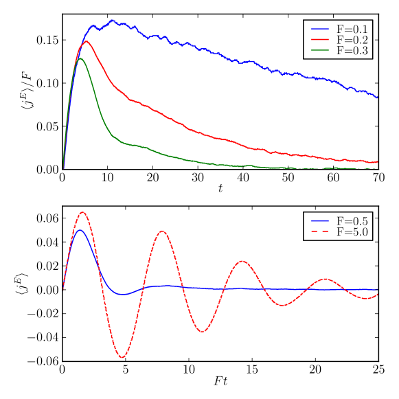
Figure 1: Time–dependence of the energy current for various electric field $F$ displayed in the legend.The system consists of $N=10$ fermions on $L=24$ sites. Under equilibrium conditions, the interactions $V=1.5$, $W=1$ correspond to a metallic state at any temperature. The results have been obtained for initial inverse temperature $\beta=0.3$.

Fig. 1 shows the time–dependence of the energy current $\langle j^{E}\rangle$ in a wire driven by low–to–moderate fields (upper panel) as well as in the strong field regime (lower panel). One can see that the ratio $\langle j^{E}\rangle/F$ is independent of the driving field at the initial stage of the evolution. It is a clear hallmark of the linear–response (LR) regime which always occurs for a sufficiently short time of driving. The stronger the field the sooner $\langle j^{E}\rangle$ departs from the predictions of the LR theory. It is not easy to obtain the $dc$ LR directly from the real–time calculations, since for any finite $F$ the long–time regime is always beyond the LR theory. The initial slope of the energy current is $\frac{\mathrm{d}}{\mathrm{d}t}\langle j^{E}\rangle_{t=0}=-F\langle\partial_{\phi}j^{E}\rangle_{t=0}$. It is interesting to note that $\langle\partial_{\phi}j^{E}\rangle_{t=0}$ is a kind of correlated hopping and represents the sum rule for LR in the initial equilibrium state.

For longer times and/or stronger $F$, the energy current diminishes and eventually vanishes. In this regime one finds a counterintuitive result when the energy current is larger when $F$ is weaker. Similar observation has previously been found for the particle currentmierzejewski2011a and explained as the result of the Joule–heating. As follows from Eq. (11) driving with electric field increases the energy of the system. This effect is beyond the LR theory hence it must be at least of the order of $F^{2}$. As soon this heating effect becomes visible it strongly depends on the magnitude of driving. Consequently two systems driven within the same time–window by different $F$ have exceedingly different energies. The system driven by weaker $F$ may be much colder hence it responds much stronger to the external driving.

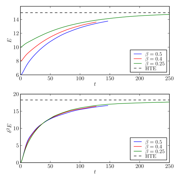
Figure 2: Time–dependence of the average energy $E(t)$ (upper panel) as well as the energy spread $\delta^{2}E$ (lower panel) for a system of $N=13$ fermions on $L=26$ sites. Here, $V=1.4$, $W=1$ and $F=0.1$ while the initial inverse temperature is indicated in the legend. The horizontal lines show the equilibrium HTE results for infinite temperature.

The time–dependence of the energy current becomes very different for even stronger fields as it is shown in the lower panel of Fig. 1. Namely, $\langle j^{E}\rangle$ starts to oscillate and this oscillations share several common features with the well known Bloch oscillations of the particle current my1 . Namely, the frequency of these oscillations is determined by the electric field while the initial amplitude of the oscillations is $F$–independent.

Finally, we discuss the time–dependence of the average energy $E(t)=\langle H(t)\rangle$ and the energy spread $\delta^{2}E=\langle[H(t)-E(t)]^{2}\rangle$. Results shown in Fig. 2 have been obtained for a system driven by a weak field. Initially, the system is in MC state, hence $\delta E\rightarrow 0$. Upon driving, $E(t)$ asymptotically approaches the energy of the system described by a the canonical ensemble with $\beta=0$. Similarly to this, also the energy spread asymptotically approaches its canonical value. However, the evolution of $\delta E$ in the low field regime is rather unexpected since it is determined mostly by the time of driving being quite independent of the instantaneous energy of the system. Such behavior contrasts with the quasiequilibrium evolution of many local observables mierzejewski2011a in the regime of low electric field. Although, the instantaneous values of the latter quantities change in time they are determined mostly by the instantaneous energy. Moreover, their expectation values are close to the equilibrium result for such ensemble that $\langle H\rangle_{equilibrium}=E(t)$. Except from the initial MC state and the asymptotic canonical one, $E(t)$ and $\delta E(t)$ are independent of each other excluding the quasiequilibrium evolution of the latter quantity. Although the behavior of the energy spread is irrelevant for macroscopic systems, it might be quite important for driven nanosystems, where the ratio $\delta E/E$ is non–negligible.

- (1) K. Matsuda, I. Hirabayashi, K. Kawamoto, T. Nabatame, T. Tokizaki, A. Nakamura, Phys. Rev. B 50, 4097 (1994)
- (2) H. Okamoto, T. Miyagoe, K. Kobayashi, H. Uemura, H. Nishioka, H. Matsuzaki, A. Sawa, Y. Tokura, Phys. Rev. B 82, 060513 (2010)
- (3) H. Okamoto, T. Miyagoe, K. Kobayashi, H. Uemura, H. Nishioka, H. Matsuzaki, A. Sawa, Y. Tokura, Phys. Rev. B 83, 125102 (2011)
- (4) Y. Taguchi, T. Matsumoto, Y. Tokura, Phys. Rev. B 62, 7015 (2000)
- (5) T. Oka, R. Arita, H. Aoki, Phys. Rev. Lett. 91, 066406 (2003)
- (6) T. Oka, H. Aoki, Phys. Rev. Lett. 95, 137601 (2005)
- (7) M. Eckstein, T. Oka, P. Werner, Phys. Rev. Lett. 105, 146404 (2010)
- (8) Z. Lenarčič, P. Prelovšek, Phys. Rev. Lett. 108, 196401 (2012)
- (9) S.R. White, A.E. Feiguin, Phys. Rev. Lett. 93, 076401 (2004)
- (10) J.K. Freericks, V.M. Turkowski, V. Zlatić, Phys. Rev. Lett. 97, 266408 (2006)
- (11) M. Mierzejewski, P. Prelovšek, Phys. Rev. Lett. 105, 186405 (2010)
- (12) M. Mierzejewski, L. Vidmar, J. Bonča, P. Prelovšek, Phys. Rev. Lett. 106, 196401 (2011)
- (13) T. Prosen, M. Žnidarič, Phys. Rev. Lett. 105, 060603 (2010)
- (14) C. Aron, G. Kotliar, C. Weber, Phys. Rev. Lett. 108, 086401 (2012)
- (15) M. Bukov, M. Heyl, Phys. Rev. B 86, 054304 (2012)
- (16) J. Bonča, M. Mierzejewski, L. Vidmar, Phys. Rev. Lett. 109, 156404 (2012)
- (17) K. Yonemitsu, N. Maeshima, T. Hasegawa, Phys. Rev. B 76, 235118 (2007)
- (18) N. Sugimoto, S. Onoda, N. Nagaosa, Phys. Rev. B 78, 155104 (2008)
- (19) A. Takahashi, H. Itoh, M. Aihara, Phys. Rev. B 77, 205105 (2008)
- (20) R. Steinigeweg, J. Herbrych, P. Prelovšek, M. Mierzejewski, Phys. Rev. B 85, 214409 (2012)
- (21) L. Vidmar, J. Bonča, T. Tohyama, S. Maekawa, Phys. Rev. Lett. 107, 246404 (2011)
- (22) L. Vidmar, J. Bonča, M. Mierzejewski, P. Prelovšek, S.A. Trugman, Phys. Rev. B 83, 134301 (2011)
- (23) M. Eckstein, P. Werner, Phys. Rev. Lett. 107, 186406 (2011)
- (24) A. Amaricci, C. Weber, M. Capone, G. Kotliar, Phys. Rev. B 86, 085110 (2012)
- (25) M. Einhellinger, A. Cojuhovschi, E. Jeckelmann, Phys. Rev. B 85, 235141 (2012)
- (26) S. Dal Conte, C. Giannetti, G. Coslovich, F. Cilento, D. Bossini, T. Abebaw, F. Banfi, G. Ferrini, H. Eisaki, M. Greven, A. Damascelli, D. van der Marel, F. Parmigiani, Science 335, 1600 (2012)
- (27) L. Rettig, R. Cortés, S. Thirupathaiah, P. Gegenwart, H.S. Jeevan, M. Wolf, J. Fink, U. Bovensiepen, Phys. Rev. Lett. 108, 097002 (2012)
- (28) F. Novelli, D. Fausti, J. Reul, F. Cilento, P.H.M. van Loosdrecht, A.A. Nugroho, T.T.M. Palstra, M. Grüninger, F. Parmigiani, Phys. Rev. B 86, 165135 (2012)
- (29) R. Cortés, L. Rettig, Y. Yoshida, H. Eisaki, M. Wolf, U. Bovensiepen, Phys. Rev. Lett. 107, 097002 (2011)
- (30) K.W. Kim, A. Pashkin, H. Schäfer, M. Beyer, M. Porer, T. Wolf, C. Bernhard, J. Demsar, R. Huber, A. Leitenstorfer, Nature Materials 11, 497 (2012)
- (31) K.A. Al-Hassanieh, F.A. Reboredo, A.E. Feiguin, I. González, E. Dagotto, Phys. Rev. Lett. 100, 166403 (2008)
- (32) N. Strohmaier, D. Greif, R. Jördens, L. Tarruell, H. Moritz, T. Esslinger, R. Sensarma, D. Pekker, E. Altman, E. Demler, Phys. Rev. Lett. 104, 080401 (2010)
- (33) R. Sensarma, D. Pekker, E. Altman, E. Demler, N. Strohmaier, D. Greif, R. Jördens, L. Tarruell, H. Moritz, T. Esslinger, Phys. Rev. B 82, 224302 (2010)
- (34) L.G.G.V. Dias da Silva, G. Alvarez, E. Dagotto, Phys. Rev. B 86, 195103 (2012)
- (35) Z. Lenarčič, P. Prelovšek, Phys. Rev. Lett. 111, 016401 (2013)
- (36) A. Takahashi, H. Gomi, M. Aihara, Phys. Rev. Lett. 89, 206402 (2002)
- (37) M. Eckstein, P. Werner, Phys. Rev. Lett. 110, 126401 (2013)
- (38) M. Leijnse, M.R. Wegewijs, K. Flensberg, Phys. Rev. B 82, 045412 (2010)
- (39) E. Muñoz, C.J. Bolech, S. Kirchner, Phys. Rev. Lett. 110, 016601 (2013)
- (40) D. Sánchez, R. López, Phys. Rev. Lett. 110, 026804 (2013)
- (41) G. Bunin, G. D’Alessio, Y. Kafri, A. Polkovnikov, Nature Physics 7, 913–917 (2011)
- (42) T. Prosen, Phys. Rev. Lett. 107, 137201 (2011)
- (43) M. Žnidarič, Phys. Rev. Lett. 106, 220601 (2011)
- (44) R. Steinigeweg, W. Brenig, Phys. Rev. Lett. 107, 250602 (2011)
- (45) M.W. Long, P. Prelovšek, S. El Shawish, J. Karadamoglou, X. Zotos, Phys. Rev. B 68, 235106 (2003)
- (46) T.J. Park, J.C. Light, The Journal of Chemical Physics 85(10), 5870 (1986)
- (47) M. Mierzejewski, J. Bonča, P. Prelovšek, Phys. Rev. Lett. 107, 126601 (2011)