RKKY interaction in bilayer graphene

Abstract

We study the RKKY interaction between two magnetic impurities located on same layer (intralayer case) or on different layers (interlayer case) in undoped bilayer graphene in the four-bands model, by directly calculating the Green functions in the eigenvalues and eigenvectors representation. Our results show that both intra- and interlayer RKKY interactions between two magnetic impurities located on same (opposite) sublattice are always ferromagnetic (antiferromagnetic). Furthermore we find unusual long-distance decay of the RKKY interaction in BLG. The intralyer RKKY interactions between two magnetic impurities located on same sublattice, $J^{A_{n}A_{n}}(\mathbf{R})$ and $J^{B_{n}B_{n}}(\mathbf{R)}$, decay closely as $1/R^{6}$ and $1/R^{2}$ at large impurity distances respectively, but when they are located on opposite sublattices the RKKY interactions exhibit $1/R^{4}$ decays approximately. In the interlayer case, the RKKY interactions between two magnetic impurities located on same sublattice show a decay close to $1/R^{4}$ at large impurity distances, but if two magnetic impurities be on opposite sublattices the RKKY interactions, $J^{A_{1}B_{2}}(\mathbf{R})$ and $J^{B_{1}A_{2}}(\mathbf{R)}$, decay closely as $1/R^{6}$ and $1/R^{2}$ respectively. Both intra- and interlayer RKKY interactions have anisotropic oscillatory factors which for intralayer case is equal to that for single layer graphene. Our results at weak and strong interlayer coupling limits reduce to the RKKY interaction of SLG and that of BLG in the two-bands approximation respectively.

¹Young Researchers and Elite Club, Kermanshah Branch, Islamic Azad University, Kermanshah, Iran

²Department of Physics, Razi University, Kermanshah, Iran

³Nano Science and Nano Technology Research Center, Razi University, Kermanshah, Iran

Keywords: Bilayer graphene; RKKY interaction; Tight-binding model; Green’s function.

1 Introduction

Graphene, since its fabrication in 2004[1], has attracted many experimental and theoretical efforts[2]. These efforts have resulted in discovery of some unconventional electronic properties such as half-integer quantum Hall effect[3, 4, 5], finite conductivity at zero charge-carrier concentration[3, 6, 7], Klein paradox[8, 9], strong suppression of weak localization[10], and Kohn anomaly[11, 12], etc. These unique properties originate from two traits of single-layer graphene (SLG), one is shrinking the Fermi surface to three pairs of points $K$ and $K^{{}^{\prime}}$ ( which are named Dirac points) at the corners of the SLG first Brillouin zone and the other is linearity of its zero gap dispersion relation near Dirac points.

The Ruderman-Kittel-Kasuya-Yosida (RKKY) interaction, the indirect exchange interaction between two magnetic impurities mediated by the itinerant electrons of the host, is a fundamental quantity of interest[13, 14, 15, 16, 17]. Recently, several groups[18, 19, 20, 21, 22, 23] have considered the RKKY interaction in SLG, by use of different methods such as directly computing the Green’s function for full tight-binding band structure[20](or for linearly dispersive band structure[20, 21]) and exact diagonalization on a finite-size lattice[19, 22], and also in different cases such as presence of the electron-electron interaction[22] or presence of the nonmagnetic disorders[23]. These works have reported two common results: one is the ferromagnetic (antiferromagnetic) order of magnetic impurities located on same (apposite) sublattices which originate from particle-hole symmetry in SLG, or each bipartite lattice, which is satisfied for nearest-neighbor interactions case. The other is the long-distance $1/R^{3}$ decay for RKKY interaction in clean SLG in contrast to the long-distance $1/R^{2}$ decay for the RKKY interaction in the ordinary two-dimensional metals. Furthermore the RKKY interaction in undoped and doped single layer graphene in the presence of a gap are also considered in Ref.[24]. This work report $1/R^{3}$ distance dependence of the RKKY interaction for undoped graphene and mixed $1/R^{2}$ and $1/R^{3}$ distance dependence for doped graphene.

More recently, simultaneous with upward tendency to scrutinize the properties of SLG, also many researchers have considered the properties of BLG[2]. BLG has a graphene-like Fermi surface besides a zero gap parabolic dispersion relation near Dirac points. In spite of these, BLG is very different from ordinary two-dimensional electron gas (2DEG) with parabolic spectrum, as well as from SLG. For example, quantum Hall effect, landau-level degeneracy and Berry phase[3, 25, 26], edge states[27], weak localization[28], Coulomb screening and collective excitations[29, 30] in BLG are different from those in the ordinary 2DEG and also from those in SLG. The RKKY interaction in BLG can signalize this difference more[31, 32, 33]. In this paper we study the RKKY interaction in undoped BLG in the four-band model, by directly computing the Green’s function in eigenvalues and eigenvectors representation. Also we discussed the RKKY interaction in BLG in the two limiting cases, weak and strong interlayer coupling. This paper is organized as follows. In section II, we introduce the model and obtain the eigenvalues and eigenvectors of BLG. The RKKY interaction formalism is introduced in section II. In section IV we present our results for intra- and interlayer RKKY interaction in BLG. Then we compare our results for the RKKY interaction with that of SLG and also with that of the ordinary 2DEG. Furthermore we discuss our results in two limiting cases, weak and strong interlayer coupling. Finally, we end this paper by summery and conclusions.

2 Model

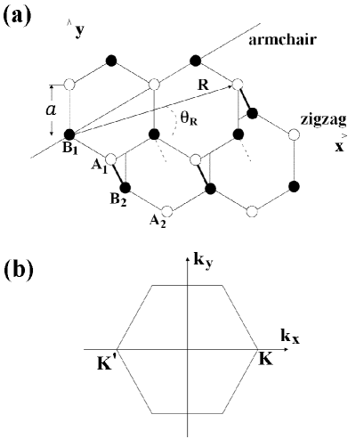
Figure 1: (a) Lattice structure of bilayer graphene, (b) corresponding Brillouin zone, with the Dirac points $\mathbf{K}=(\frac{4\pi}{3\sqrt{3}a},0)$ and $\mathbf{K}^{{}^{\prime}}=(-\frac{4\pi}{3\sqrt{3}a},0)$ indicated.

The BLG (Figure 1 (a)) is composed of a pair of hexagonal networks of carbon atoms, with $A_{1}$ and $B_{1}$ symmetries on top layer and $A_{2}$ and $B_{2}$ on bottom one. $A_{1}$ atoms are located above $B_{2}$ atoms and $B_{1}$ atoms are above the center of hexagons in bottom layer. Let us model the BLG with only two parameters $t$ and $\gamma$, where $t=2.7eV$ and $\gamma=0.39eV$ which present the nearest neighbor intralayer ($A_{1}\longleftrightarrow B_{1}$ or $A_{2}\longleftrightarrow B_{2}$) and interlayer ($A_{1}\longleftrightarrow B_{2}$) couplings between $\pi$ electrons respectively.

The low energy states of $\pi$ electrons in BLG is given by the states around the $\mathbf{K}$ and $\mathbf{K}^{{}^{\prime}}$ points (Figure 1 (b)) and can be described by a Hamiltonian as

$$\widehat{H}(\mathbf{k})=\left(\begin{array}[]{cccc}0&\xi v_{F}(k_{x}+\xi ik_{y})&0&\gamma\\ \xi v_{F}(k_{x}-\xi ik_{y})&0&0&0\\ 0&0&0&\xi v_{F}(k_{x}+\xi ik_{y})\\ \gamma&0&\xi v_{F}(k_{x}-\xi ik_{y})&0\\ \end{array}\right),$$ (1)

which operates in the space of four components wave functions,

$$\widehat{\Psi}(\mathbf{k})=\left(\begin{array}[]{c}\psi^{A_{1}}(\mathbf{k})\\ \psi^{B_{1}}(\mathbf{k})\\ \psi^{A_{2}}(\mathbf{k})\\ \psi^{B_{2}}(\mathbf{k})\\ \end{array}\right),$$ (2)

where $\psi^{\alpha}(\mathbf{k})$ is the electron amplitude on the sublattice $\alpha$ with $\mathbf{k}$ in the valley $\mathbf{K}(\mathbf{K}^{{}^{\prime}})$. $\mathbf{k}=(k_{x},k_{y})$, two dimensional momentum, is measured relative to the valley $\mathbf{K}(\mathbf{K}^{{}^{\prime}})$ if $\xi$ be $+1(-1)$ and $v_{F}=\frac{3}{2}ta$ is the Fermi velocity, where $a$ is the shortest carbon-carbon distance.

BLG Schrodinger equation,

$$(\widehat{H}(\mathbf{k})-E\mathbf{\widehat{1}})\widehat{\Psi}(\mathbf{k})=0,$$ (3)

could be solved to obtain the energy bands as[34],

$$E_{\lambda}^{\nu}=\nu(\sqrt{(v_{F}k)^{2}+(\frac{\gamma}{2})^{2}}+(-1)^{\lambda}\frac{\gamma}{2}),$$ (4)

where $\lambda=1,2$ are the energy bands number and $\nu=+(-)$ indicates the conduction(valance) energy bands respectively. By using eigenvalues, equation (4), we obtain their appropriate wave functions

$$\widehat{\Psi}_{\mathbf{K}\lambda\nu}(\mathbf{k})=\left(\begin{array}[]{c}\psi^{A_{1}}_{\mathbf{K}\lambda\nu}(\mathbf{k})\\ \psi^{B_{1}}_{\mathbf{K}\lambda\nu}(\mathbf{k})\\ \psi^{A_{2}}_{\mathbf{K}\lambda\nu}(\mathbf{k})\\ \psi^{B_{2}}_{\mathbf{K}\lambda\nu}(\mathbf{k})\\ \end{array}\right)=\frac{1}{\sqrt{2}\sqrt{(E_{\lambda}^{\nu})^{2}+(v_{F}k)^{2}}}\left(\begin{array}[]{c}E_{\lambda}^{\nu}e^{+i{\theta}_{\mathbf{k}}}\\ v_{F}k\\ \nu(-1)^{\lambda}v_{F}k\\ \nu(-1)^{\lambda}E_{\lambda}^{\nu}e^{-i{\theta}_{\mathbf{k}}}\end{array}\right),$$ (5)

with $\mathbf{k}$ in the valley $\mathbf{K}$ and

$$\widehat{\Psi}_{\mathbf{K}^{{}^{\prime}}\lambda\nu}(\mathbf{k})=\left(\begin{array}[]{c}\psi^{A_{1}}_{\mathbf{K}^{{}^{\prime}}\lambda\nu}(\mathbf{k})\\ \psi^{B_{1}}_{\mathbf{K}^{{}^{\prime}}\lambda\nu}(\mathbf{k})\\ \psi^{A_{2}}_{\mathbf{K}^{{}^{\prime}}\lambda\nu}(\mathbf{k})\\ \psi^{B_{2}}_{\mathbf{K}^{{}^{\prime}}\lambda\nu}(\mathbf{k})\\ \end{array}\right)=\frac{1}{\sqrt{2}\sqrt{(E_{\lambda}^{\nu})^{2}+(v_{F}k)^{2}}}\left(\begin{array}[]{c}E_{\lambda}^{\nu}e^{-i{\theta}_{\mathbf{k}}}\\ -v_{F}k\\ -\nu(-1)^{\lambda}v_{F}k\\ \nu(-1)^{\lambda}E_{\lambda}^{\nu}e^{+i{\theta}_{\mathbf{k}}}\end{array}\right),$$ (6)

with $\mathbf{k}$ in the valley $\mathbf{K}^{{}^{\prime}}$, where ${\theta}_{\mathbf{k}}=tan^{-1}(\frac{k_{y}}{k_{x}})$.

3 RKKY formalism

In this section we introduce the RKKY formalism for BLG. Let us consider two magnetic impurities located on the sublattices $\alpha$ and $\beta$ in the sites i and j respectively, that have a small on site spin exchange interaction with the itinerant electrons as

$$H_{int}=-g\mathbf{S}_{i\alpha}\mathbf{.}\mathbf{s}_{i\alpha}-g\mathbf{S}_{j\beta}\mathbf{.}\mathbf{s}_{j\beta},$$ (7)

where $g$ is the coupling constant between the localized magnetic impurities and the itinerant electrons ($g\ll t$ and $\gamma$), $\mathbf{S}_{i\alpha}$ is the spin of the magnetic impurity located at the sublattice $\alpha$ in site i, $\mathbf{s}_{i\alpha}=\frac{1}{2}c_{i\sigma}^{\alpha{\dagger}}\mathbf{\sigma}_{\sigma\sigma^{{}^{\prime}}}c_{i\sigma^{{}^{\prime}}}^{\alpha}$ is the spin of the itinerant electrons. By use of the perturbation theory for the thermodynamic potential[35], up to the second-order of $H_{int}$ and by ignoring all terms proportional to $\mathbf{S}_{i\alpha}^{2}$ and $\mathbf{S}_{j\beta}^{2}$, one can obtain following relation

$$H_{RKKY}=-J_{ij}^{\alpha\beta}\mathbf{S}_{i\alpha}\mathbf{.}\mathbf{S}_{j\beta},$$ (8)

where $J_{ij}^{\alpha\beta}$ is the RKKY interaction between two magnetic impurities located on sublattices $\alpha$ and $\beta$ in sites i and j respectively. This is given by[21, 36]

$$J_{ij}^{\alpha\beta}=-\frac{g^{2}}{4}\int_{0}^{\frac{1}{T}}G^{\alpha\beta}(i,j,\tau)G^{\beta\alpha}(j,i,-\tau),$$ (9)

where $G^{\alpha\beta}(i,j,\tau)$ for BLG could be written in the eigenvectors and eigenvalues representation as

$$G^{\alpha\beta}(i,j,\tau) = \frac{s}{\Omega_{BZ}}\sum_{\lambda,\nu}\int d^{2}\mathbf{k}[$$ (10)

$$( e^{+i(\mathbf{K}+\mathbf{k}).\mathbf{R}_{i}}\psi_{\mathbf{K}\lambda\nu}^{\alpha})^{\ast}(e^{+i(\mathbf{K}+\mathbf{k}).\mathbf{R}_{j}}\psi^{\beta}_{\mathbf{K}\lambda\nu})+(e^{+i(\mathbf{K}^{{}^{\prime}}+\mathbf{k}).\mathbf{R}_{i}}\psi_{\mathbf{K}^{{}^{\prime}}\lambda\nu}^{\alpha})^{\ast}(e^{+i(\mathbf{K}^{{}^{\prime}}+\mathbf{k}).\mathbf{R}_{j}}\psi^{\beta}_{\mathbf{K}^{{}^{\prime}}\lambda\nu})]$$

$$\times e^{-\xi_{\lambda\nu}(k)\tau}(-(1-n_{F}(\xi_{\lambda\nu}(k)))\theta(\tau)+n_{F}(\xi_{\lambda\nu}(k))\theta(-\tau)),$$

where $\xi_{\lambda\nu}=E_{\lambda}^{\nu}-\mu$, $n_{F}(\xi_{\lambda\nu})=(1+e^{\beta\xi_{\lambda\nu}})^{-1}$ is the Fermi distribution function, $s=2$ is the spin degeneracy and $\Omega_{BZ}=\frac{2(2\pi)^{2}}{3\sqrt{3}a^{2}}$ is the area of the first Brillouin zone. In the next section, by use of this formalism, we consider the RKKY interaction in BLG.

4 Results and discussion

We apply the introduced RKKY formalism to all possible configurations of two magnetic impurities located on BLG. These two magnetic impurities could be on same layer (intralayer interaction case) or on different layers (interlayer interaction case). For each case, two impurities could be on same sublattice or on different sublattices. So overall we have four possible configurations. In the next subsections for these configurations we calculate the RKKY interactions from obtained relations of previous section, equations (8)-(10).

4.1 Magnetic impurities on same sublattice for intralayer case

We now calculate intralayer RKKY interaction between magnetic impurities located on same sublattice in the undoped BLG ($\mu=0$) at $T=0$. For this, first we must obtain the required Green’s functions from equations (4)-(6) and (9)-(10). Equations (5), (6) and (10) show that for BLG we have $G^{A_{1}A_{1}}(i,j,\tau)=G^{B_{2}B_{2}}(i,j,\tau)$ and $G^{B_{1}B_{1}}(i,j,\tau)=G^{A_{2}A_{2}}(i,j,\tau)$[37]. So, $J^{A_{1}A_{1}}(\mathbf{R}_{ij})=J^{B_{2}B_{2}}(\mathbf{R}_{ij})$ and $J^{B_{1}B_{1}}(\mathbf{R}_{ij})=J^{A_{2}A_{2}}(\mathbf{R}_{ij})$ but $J^{A_{1}A_{1}}(\mathbf{R}_{ij})\neq J^{B_{1}B_{1}}(\mathbf{R}_{ij})$, hence they must be calculated separately. The required Green’s functions to calculate $J^{A_{1}A_{1}}(\mathbf{R}_{ij})$ are

$$G^{A_{1}A_{1}}(i,j,\tau)=-\frac{1}{\Omega_{BZ}}(e^{-i\mathbf{K}.\mathbf{R}_{ij}}+e^{-i\mathbf{K}^{{}^{\prime}}.\mathbf{R}_{ij}})\int d^{2}\mathbf{k}e^{-i\mathbf{k}.\mathbf{R}_{ij}}($$

$$\frac{(E_{1}^{+})^{2}}{(E_{1}^{+})^{2}+(v_{F}k)^{2}}e^{-E_{1}^{+}\tau}+\frac{(E_{2}^{+})^{2}}{(E_{2}^{+})^{2}+(v_{F}k)^{2}}e^{-E_{2}^{+}\tau}),$$ (11)

and

$$G^{A_{1}A_{1}}(j,i,-\tau)=\frac{1}{\Omega_{BZ}}(e^{+i\mathbf{K}.\mathbf{R}_{ij}}+e^{+i\mathbf{K}^{{}^{\prime}}.\mathbf{R}_{ij}})\int d^{2}\mathbf{k}e^{+i\mathbf{k}.\mathbf{R}_{ij}}($$

$$\frac{(E_{1}^{+})^{2}}{(E_{1}^{+})^{2}+(v_{F}k)^{2}}e^{-E_{1}^{+}\tau}+\frac{(E_{2}^{+})^{2}}{(E_{2}^{+})^{2}+(v_{F}k)^{2}}e^{-E_{2}^{+}\tau}).$$ (12)

By performing the angle integration of equations (11) and (12) we obtain

$$G^{A_{1}A_{1}}(i,j,\tau)=-\frac{2\pi}{\Omega_{BZ}}(e^{-i\mathbf{K}.\mathbf{R}_{ij}}+e^{-i\mathbf{K}^{{}^{\prime}}.\mathbf{R}_{ij}})\int_{0}^{\infty}kdkJ_{0}(kR)($$

$$\frac{(E_{1}^{+})^{2}}{(E_{1}^{+})^{2}+(v_{F}k)^{2}}e^{-E_{1}^{+}\tau}+\frac{(E_{2}^{+})^{2}}{(E_{2}^{+})^{2}+(v_{F}k)^{2}}e^{-E_{2}^{+}\tau}),$$ (13)

and

$$G^{A_{1}A_{1}}(j,i,-\tau)=\frac{2\pi}{\Omega_{BZ}}(e^{+i\mathbf{K}.\mathbf{R}_{ij}}+e^{+i\mathbf{K}^{{}^{\prime}}.\mathbf{R}_{ij}})\int_{0}^{\infty}kdkJ_{0}(kR)($$

$$\frac{(E_{1}^{+})^{2}}{(E_{1}^{+})^{2}+(v_{F}k)^{2}}e^{-E_{1}^{+}\tau}+\frac{(E_{2}^{+})^{2}}{(E_{2}^{+})^{2}+(v_{F}k)^{2}}e^{-E_{2}^{+}\tau}),$$ (14)

where $J_{0}$ is Bessel function of the zero order, $\mathbf{R}_{ij}$ is a vector drawn from site i to site j and $R=|\mathbf{R}_{ij}|$. If we substitute these equations into equation (9) and replace variables $k$ and $\tau$ with $x=kR$ and $y=\frac{v_{F}}{R}\tau$ respectively, we obtain following relation for $J^{A_{1}A_{1}}(\mathbf{R}_{ij})$

$$J^{A_{1}A_{1}}(\mathbf{R}_{ij})=\frac{9g^{2}}{64\pi^{2}t}\frac{1+cos[(\mathbf{K}-\mathbf{K}^{{}^{\prime}}).\mathbf{R}_{ij}]}{(R/a)^{3}}\int_{0}^{\infty}dy[\int_{0}^{\infty}xdxJ_{0}(x)($$

$$\frac{\varepsilon_{1}}{\sqrt{x^{2}+(\frac{\gamma}{3t}\frac{R}{a})^{2}}}e^{-\varepsilon_{1}y}+\frac{\varepsilon_{2}}{\sqrt{x^{2}+(\frac{\gamma}{3t}\frac{R}{a})^{2}}}e^{-\varepsilon_{2}y})]^{2},$$ (15)

where $\varepsilon_{1}=\sqrt{x^{2}+(\frac{\gamma}{3t}\frac{R}{a})^{2}}-\frac{\gamma}{3t}\frac{R}{a}$, $\varepsilon_{2}=\sqrt{x^{2}+(\frac{\gamma}{3t}\frac{R}{a})^{2}}+\frac{\gamma}{3t}\frac{R}{a}$ and $R$ is the distance between two magnetic impurities. Also by calculating $G^{B_{1}B_{1}}(i,j,\tau)$ and $G^{B_{1}B_{1}}(j,i,-\tau)$ and substituting them into equation (9) we obtain following relation for $J^{B_{1}B_{1}}(\mathbf{R}_{ij})$

$$J^{B_{1}B_{1}}(\mathbf{R}_{ij})=\frac{9g^{2}}{16\pi^{2}t}\frac{1+cos[(\mathbf{K}-\mathbf{K}^{{}^{\prime}}).\mathbf{R}_{ij}]}{(R/a)^{3}}\int_{0}^{\infty}dy[\int_{0}^{\infty}xdxJ_{0}(x)($$

$$\frac{x^{2}}{\varepsilon_{1}^{2}+x^{2}}e^{-\varepsilon_{1}y}+\frac{x^{2}}{\varepsilon_{2}^{2}+x^{2}}e^{-\varepsilon_{2}y})]^{2}.$$ (16)

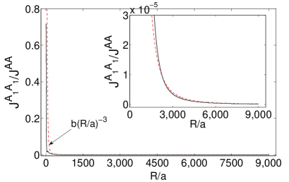
Figure 2: Plot of $J^{A_{1}A_{1}}(\mathbf{R}_{ij})$ in units of $J^{AA}(\mathbf{R}_{ij})$ (black solid line) fitted to $\frac{b}{(R/a)^{3}}$ curve (red dashed line) as a function of $R/a$ where $b=109950$.

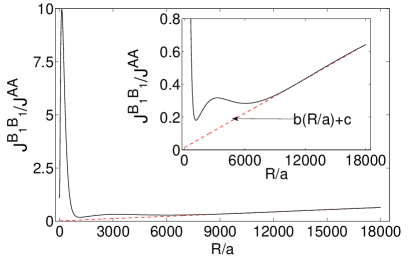
Figure 3: Plot of $J^{B_{1}B_{1}}(\mathbf{R}_{ij})$ in units of $J^{BB}(\mathbf{R}_{ij})$ (black solid line) fitted to $b\frac{R}{a}+c$ line (red dashed line) as a function of $R/a$ where $b=0.000035$ and $c=0.0142$.

The result of the integrals in equations (15) and (16) are always positive. Therefore the intralayer RKKY interactions between magnetic impurities located on same sublattice in BLG are always ferromagnetic. This is similar to the ferromagnetic coupling between magnetic moments located on same sublattice in SLG[18, 20, 21, 19]. Also the intralayer RKKY interactions of BLG, $J^{A_{1}A_{1}}(\mathbf{R}_{ij})$ and $J^{B_{1}B_{1}}(\mathbf{R}_{ij})$, show anisotropic $1+cos[(\mathbf{K}-\mathbf{K}^{{}^{\prime}}).\mathbf{R}_{ij}]$-type oscillations which are similar to that of SLG[18, 20, 21, 19]. But the $R$ dependent features of the intralayer RKKY interactions of BLG and that of SLG are different, besides the difference between the $R$ dependence of $J^{A_{1}A_{1}}(\mathbf{R}_{ij})$ and $J^{B_{1}B_{1}}(\mathbf{R}_{ij})$. The $R$ dependence of the RKKY interactions of BLG, equations (15) and (16), could not be determined analytically. Hence to specify the $R$ dependent behavior of $J^{A_{1}A_{1}}(\mathbf{R}_{ij})$ and $J^{B_{1}B_{1}}(\mathbf{R}_{ij})$ and compare them with the $R$ dependent behavior of RKKY interaction in SLG, we calculate them from equations (15) and (16) numerically and plot them in units of $J^{AA}(\mathbf{R}_{ij})$ of SLG. Plots of $J^{A_{1}A_{1}}(\mathbf{R}_{ij})$ and $J^{B_{1}B_{1}}(\mathbf{R}_{ij})$ in units of $J^{AA}(\mathbf{R}_{ij})$ have been shown in figures 2 and 3 respectively. Note that the $R$ dependence of these plots is independent of direction of $\mathbf{R}_{ij}$(Figure 1), since the intralayer RKKY interactions of BLG and SLG have same oscillatory factor.

Figure 2 shows that the intralayer RKKY interaction between magnetic impurities located on same sublattice $A_{1}$, $J^{A_{1}A_{1}}(\mathbf{R}_{ij})$, always is weaker than that of SLG for all impurity distances ($J^{A_{1}A_{1}}(\mathbf{R}_{ij})<J^{AA}(\mathbf{R}_{ij})$). Furthermore $J^{A_{1}A_{1}}(\mathbf{R}_{ij})$ at small and large distances falls off faster than $1/R^{3}$, the power law decay of RKKY interaction of SLG[18, 20, 21, 19, 24], specially at large impurity distances, $J^{A_{1}A_{1}}(\mathbf{R}_{ij})$ decays approximately as $1/R^{6}$. This behavior of $J^{A_{1}A_{1}}(\mathbf{R}_{ij})$ is unlike the long-distances behavior of the RKKY interaction of SLG, $1/R^{3}$, and also unlike the long-distances behavior of the RKKY interaction of ordinary 2DEG, $1/R^{2}$.

From figure 3 we see that at small impurity distances, $R$, by increasing $R$ first $J^{B_{1}B_{1}}(\mathbf{R}_{ij})/J_{AA}(\mathbf{R}_{ij})$ increases which means $J^{B_{1}B_{1}}(\mathbf{R}_{ij})$ falls of smoother than $1/R^{3}$. After approaching to a maximum amount then it decreases which means that $J^{B_{1}B_{1}}(\mathbf{R}_{ij})$ decays faster than $1/R^{3}$. By increasing the impurity distances this behavior repeats again but with smaller maximum amount. At very large impurity distances, $J^{B_{1}B{1}}(\mathbf{R}_{ij})$ shows a decay close to $1/R^{2}$ which is similar to the long-distance behavior of the RKKY interaction in the ordinary 2DEG[17]. Also comparison of figures 2 and 3 exhibit that for all impurity distances, $J^{B_{1}B_{1}}(\mathbf{R}_{ij})>J^{A_{1}A_{1}}(\mathbf{R}_{ij})$. This could be explain in terms of difference of the local density of states at $A_{1}$ and $B_{1}$ sublattices. Note that the local density of states of BLG at sublattice $A_{1}$ is $\frac{S|E|}{\pi v^{2}_{F}}$ for $|E|>\gamma$ and $\frac{S|E|}{2\pi v^{2}_{F}}$ for $|E|<\gamma$ while he local density of states of BLG at sublattice $B_{1}$ is $\frac{S|E|}{\pi v^{2}_{F}}$ for $|E|>\gamma$ and $\frac{S(|E|+\gamma)}{2\pi v^{2}_{F}}$ for $|E|<\gamma$[37] where $E$ is energy and $S$ is the area of unit cell in real space. So the indirect RKKY interaction mediated by itinerant electrons, which depends on density of states, behaves as $J^{B_{1}B_{1}}(\mathbf{R}_{ij})>J^{A_{1}A_{1}}(\mathbf{R}_{ij})$.

Let us now discus our results for the intralayer RKKY interactions of BLG in the two limiting cases, the weak interlayer coupling ($\gamma\rightarrow 0$) and the strong interlayer coupling ($\gamma\rightarrow\infty$). In the first limiting case, $\gamma\rightarrow 0$, we obtain following results for intralayer RKKY interactions of BLG

$$J^{A_{1}A_{1}}(\mathbf{R}_{ij})=\frac{9g^{2}}{64\pi^{2}t}\frac{1+cos[(\mathbf{K}-\mathbf{K}^{{}^{\prime}}).\mathbf{R}_{ij}]}{(R/a)^{3}}\int_{0}^{\infty}dy[\int_{0}^{\infty}xdxJ_{0}(x)(e^{-xy}+e^{-xy})]^{2},$$ (17)

and

$$J^{B_{1}B_{1}}(\mathbf{R}_{ij})=\frac{9g^{2}}{16\pi^{2}t}\frac{1+cos[(\mathbf{K}-\mathbf{K}^{{}^{\prime}}).\mathbf{R}_{ij}]}{(R/a)^{3}}\int_{0}^{\infty}dy[\int_{0}^{\infty}xdxJ_{0}(x)(\frac{e^{-xy}}{2}+\frac{e^{-xy}}{2}]^{2},$$ (18)

which after performing the integrals[21, 38, 39] can be written as

$$J^{A_{1}A_{1}}(\mathbf{R}_{ij})=J^{B_{1}B_{1}}(\mathbf{R}_{ij})=\frac{9g^{2}}{256\pi t}\frac{1+cos[(\mathbf{K}-\mathbf{K}^{{}^{\prime}}).\mathbf{R}_{ij}]}{(R/a)^{3}},$$ (19)

that is equal to equation 23 of Ref. 20 for the RKKY interaction between magnetic impurities located on same sublattices in SLG.

In the second limiting case, $\frac{v_{F}k}{\gamma}\rightarrow 0$, the low energy states of BLG are characterized by[34, 40],

$$E_{1\nu}=\nu\frac{\gamma}{2}((1+\frac{4v^{2}_{F}k^{2}}{\gamma^{2}})^{\frac{1}{2}}-1)\simeq\nu\frac{(v_{F}k)^{2}}{\gamma}.$$ (20)

Since the low energy states are localized on $B_{1}$ and $A_{2}$ sites[34], we only discuss the RKKY interaction between magnetic impurities located on sublattices $B_{1}$ and $A_{2}$, namely $J^{B_{1}B_{1}},J^{A_{2}A_{2}}$, $J^{B_{1}A_{2}}$, and $J^{A_{2}B_{1}}$. We follow the method introduced in this subsection to obtain the RKKY interaction, but replace variables $k$ and $\tau$ with $x=kR$ and $y=\frac{v_{F}^{2}}{\gamma R^{2}}\tau$ respectively while the terms $x/(\frac{2\gamma}{3t}\frac{R}{a})$ and $e^{-\frac{2\gamma}{3t}\frac{R}{a}}$ are ignored. Hence we get following results for $J^{A_{1}A_{1}}(\mathbf{R}_{ij})$ and $J^{B_{2}B_{2}}(\mathbf{R}_{ij})$,

$$J^{B_{1}B_{1}}(\mathbf{R}_{ij})=J^{A_{2}A_{2}}(\mathbf{R}_{ij})=\frac{27mg^{2}a^{4}}{16\pi^{2}}\frac{1+cos[(\mathbf{K}-\mathbf{K}^{{}^{\prime}}).\mathbf{R}_{ij}]}{R^{2}}\int_{0}^{\infty}dy[$$

$$\int_{0}^{\infty}xdxJ_{0}(x)e^{-x^{2}y}]^{2},$$ (21)

where $m=\frac{\gamma}{2v_{F}^{2}}$ is the electron effective mass[34, 40]. The integral can be performed easily[21, 41, 42] and the equation (21) can be written as

$$J^{B_{1}B_{1}}(\mathbf{R}_{ij})=J^{A_{2}A_{2}}(\mathbf{R}_{ij})=\frac{27mg^{2}a^{4}}{32\pi^{2}}\frac{1+cos[(\mathbf{K}-\mathbf{K}^{{}^{\prime}}).\mathbf{R}_{ij}]}{R^{2}}.$$ (22)

This result is the same as equation 38 of Ref.21 but with an extra scaling factor $\frac{27}{2}$.

4.2 Magnetic impurities on different sublattices for intralayer case

Now we calculate the RKKY interaction, $J^{\alpha\beta}(\mathbf{R}_{ij})$, when $\alpha$ and $\beta$ are different sublattices in a same layer. In this case all Green’s functions, $G^{\alpha\beta}(i,j,\tau)$, and therefore all corresponding intralayer RKKY interactions, $J^{\alpha\beta}(\mathbf{R}_{ij})$, are equal, so it is enough to calculate one of them. As an example we calculate $J^{A_{1}B_{1}}(\mathbf{R}_{ij})$. The required Green’s functions to calculate $J^{A_{1}B_{1}}(\mathbf{R}_{ij})$ are

$$G^{A_{1}B_{1}}(i,j,\tau)=\frac{1}{\Omega_{BZ}}\int d^{2}\mathbf{k}e^{-i\mathbf{k}.\mathbf{R}_{ij}}(e^{-i(\mathbf{K}^{{}^{\prime}}.\mathbf{R}_{ij}-\theta_{\mathbf{k}})}-e^{-i(\mathbf{K}^{.}\mathbf{R}_{ij}+\theta_{\mathbf{k}})})($$

$$\frac{v_{F}kE_{1}^{+}}{(E_{1}^{+})^{2}+(v_{F}k)^{2}}e^{-E_{1}^{+}\tau}+\frac{v_{F}kE_{2}^{+}}{(E_{2}^{+})^{2}+(v_{F}k)^{2}}e^{-E_{2}^{+}\tau}),$$ (23)

and

$$G^{B_{1}A_{1}}(j,i,-\tau)=\frac{1}{\Omega_{BZ}}\int d^{2}\mathbf{k}e^{+i\mathbf{k}.\mathbf{R}_{ij}}(e^{+i(\mathbf{K}^{{}^{\prime}}.\mathbf{R}_{ij}-\theta_{\mathbf{k}})}-e^{+i(\mathbf{K}^{.}\mathbf{R}_{ij}+\theta_{\mathbf{k}})})($$

$$\frac{v_{F}kE_{1}^{+}}{(E_{1}^{+})^{2}+(v_{F}k)^{2}}e^{-E_{1}^{+}\tau}+\frac{v_{F}kE_{2}^{+}}{(E_{2}^{+})^{2}+(v_{F}k)^{2}}e^{-E_{2}^{+}\tau}).$$ (24)

After the angle integration we get

$$G^{A_{1}B_{1}}(i,j,\tau)=\frac{2\pi}{\Omega_{BZ}}(e^{-i(\mathbf{K}^{{}^{\prime}}.\mathbf{R}_{ij}-\theta_{\mathbf{R}})}-e^{-i(\mathbf{K}^{.}\mathbf{R}_{ij}+\theta_{\mathbf{R}})})\int_{0}^{\infty}kdkJ_{1}(kR)($$

$$\frac{v_{F}kE_{1}^{+}}{(E_{1}^{+})^{2}+(v_{F}k)^{2}}e^{-E_{1}^{+}\tau}+\frac{v_{F}kE_{2}^{+}}{(E_{2}^{+})^{2}+(v_{F}k)^{2}}e^{-E_{2}^{+}\tau}),$$ (25)

and

$$G^{B_{1}A_{1}}(j,i,-\tau)=\frac{2\pi}{\Omega_{BZ}}e^{+i(\mathbf{K}^{{}^{\prime}}.\mathbf{R}_{ij}-\theta_{\mathbf{R}})}-e^{+i(\mathbf{K}^{.}\mathbf{R}_{ij}+\theta_{\mathbf{R}})})\int_{0}^{\infty}kdkJ_{1}(kR)($$

$$\frac{v_{F}kE_{1}^{+}}{(E_{1}^{+})^{2}+(v_{F}k)^{2}}e^{-E_{1}^{+}\tau}+\frac{v_{F}kE_{2}^{+}}{(E_{2}^{+})^{2}+(v_{F}k)^{2}}e^{-E_{2}^{+}\tau}),$$ (26)

where $J_{1}(x)$ is the Bessel function of first order and $\theta_{\mathbf{R}}$ is the angle between $\mathbf{K}-\mathbf{K}^{{}^{\prime}}$ and $\mathbf{R}_{ij}$. By substituting these equations into equation (9), we obtain

$$J^{A_{1}B_{1}}(\mathbf{R}_{ij})=-\frac{9g^{2}}{64\pi^{2}t}\frac{1-cos[(\mathbf{K}-\mathbf{K}^{{}^{\prime}}).\mathbf{R}_{ij}+2\theta_{\mathbf{R}}]}{(R/a)^{3}}\int_{0}^{\infty}dy[\int_{0}^{\infty}xdxJ_{1}(x)($$

$$\frac{x}{\sqrt{x^{2}+(\frac{\gamma}{3t}\frac{R}{a})^{2}}}e^{-\varepsilon_{1}y}+\frac{x}{\sqrt{x^{2}+(\frac{\gamma}{3t}\frac{R}{a})^{2}}}e^{-\varepsilon_{2}y})]^{2}.$$ (27)

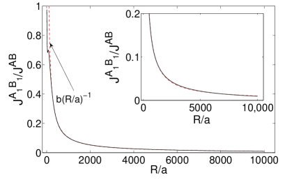
Figure 4: Plot of the $J^{A_{1}B_{1}}(\mathbf{R}_{ij})$ in units of $J^{AB}(\mathbf{R}_{ij})$ (black solid line) fitted to $\frac{b}{(R/a)}$ curve (red dashed line) as a function of $R/a$ where $b=103$.

We see that, similar to SLG, the intralayer RKKY interaction between magnetic impurities located on different sublattices in BLG is also negative, which indicate an antiferromagnetic RKKY interaction between them. Also our result for the intralayer RKKY interaction has an oscillatory factor, $1-cos[(\mathbf{K}-\mathbf{K}^{{}^{\prime}}).\mathbf{R}_{ij}+2\theta_{\mathbf{R}}]$, which is equal to that of $J^{AB}(\mathbf{R}_{ij})$ in SLG[20](Note that $J^{A_{1}B_{1}}(\mathbf{R}_{ij})=J^{B_{1}A_{1}}(-\mathbf{R}_{ij}$)). To specify the $R$ dependent behavior of the intralayer RKKY interaction in BLG we calculate it from equation (27) numerically and plot it in units of $J^{AB}(\mathbf{R}_{ij})$ of SLG. This has been shown in figure 4. We see that for all impurity distances, the RKKY interaction between magnetic impurities located on different sublattices in BLG is less than that of SLG. Furthermore figure 4 shows that at large impurity distances $J^{A_{1}B_{1}}(\mathbf{R}_{ij})$ falls off as $1/R^{4}$ approximately. This behavior is unlike the long-distances $1/R^{3}$ decay of the RKKY interaction in SLG[18, 20, 21, 19, 24] and also unlike the long-distances $1/R^{2}$ decay of the RKKY interaction in 2DEG[17]. Similar result for power law decay of $J^{A_{1}B_{1}}(\mathbf{R}_{ij})$ has been reported in Ref.31.

In the weak interlayer coupling limit, $\gamma\rightarrow 0$, we obtain following result for intralayer RKKY interactions of BLG

$$J^{A_{1}B_{1}}(\mathbf{R}_{ij})=-\frac{9g^{2}}{16\pi^{2}t}\frac{1-cos[(\mathbf{K}-\mathbf{K}^{{}^{\prime}}).\mathbf{R}_{ij}+2\theta_{\mathbf{R}}]}{(R/a)^{3}}\int_{0}^{\infty}dy[\int_{0}^{\infty}xdxJ_{1}(x)(\frac{e^{-xy}}{2}+\frac{e^{-xy}}{2}]^{2},$$ (28)

which after performing the integrals[39] can be written as

$$J^{A_{1}B_{1}}(\mathbf{R}_{ij})=-\frac{27g^{2}}{256\pi t}\frac{1-cos[(\mathbf{K}-\mathbf{K}^{{}^{\prime}}).\mathbf{R}_{ij}+2\theta_{\mathbf{R}}]}{(R/a)^{3}},$$ (29)

that is equal to equation 30 of Ref. 20 for the RKKY interaction between magnetic impurities located on opposite sublattices in SLG. Also note that $J^{A_{1}B_{1}}(\mathbf{R}_{ij})=J^{B_{1}A_{1}}(-\mathbf{R}_{ij})$.

4.3 Magnetic impurities on same sublattice for interlayer case

In this subsection we calculate interlayer RKKY interaction between magnetic impurities located on same sublattice namely $J^{\alpha_{1}\alpha_{2}}(\mathbf{R}_{ij})$ where $\alpha$ is $A$ or $B$. Similar to the previous subsections, first we calculate the required Green’s functions, $G^{\alpha_{1}\alpha_{2}}(i,j,\tau)$, where for sublattice $\alpha=A$ they are

$$G^{A_{1}A_{2}}(i,j,\tau)=-\frac{2\pi}{\Omega_{BZ}}(e^{-i(\mathbf{K}^{{}^{\prime}}.\mathbf{R}_{ij}-\theta_{\mathbf{R}})}-e^{-i(\mathbf{K}^{.}\mathbf{R}_{ij}+\theta_{\mathbf{R}})})\int_{0}^{\infty}kdkJ_{1}(kR)($$

$$\frac{v_{F}kE_{1}^{+}}{(E_{1}^{+})^{2}+(v_{F}k)^{2}}e^{-E_{1}^{+}\tau}+\frac{v_{F}kE_{2}^{+}}{(E_{2}^{+})^{2}+(v_{F}k)^{2}}e^{-E_{2}^{+}\tau}),$$ (30)

and

$$G^{A_{2}A_{1}}(i,j,-\tau)=\frac{2\pi}{\Omega_{BZ}}(e^{+i(\mathbf{K}^{{}^{\prime}}.\mathbf{R}_{ij}-\theta_{\mathbf{R}})}-e^{+i(\mathbf{K}^{.}\mathbf{R}_{ij}+\theta_{\mathbf{R}})})\int_{0}^{\infty}kdkJ_{1}(kR)($$

$$\frac{v_{F}kE_{1}^{+}}{(E_{1}^{+})^{2}+(v_{F}k)^{2}}e^{-E_{1}^{+}\tau}+\frac{v_{F}kE_{2}^{+}}{(E_{2}^{+})^{2}+(v_{F}k)^{2}}e^{-E_{2}^{+}\tau}).$$ (31)

If we substitute equations (30) and (31) into equation (9), we obtain following relation for $J^{A_{1}A_{2}}(\mathbf{R})$

$$J^{A_{1}A_{2}}(\mathbf{R}_{ij})=\frac{9g^{2}}{64\pi^{2}t}\frac{1-cos[(\mathbf{K}-\mathbf{K}^{{}^{\prime}}).\mathbf{R}_{ij}+2\theta_{\mathbf{R}}]}{(R/a)^{3}}\int_{0}^{\infty}dy[\int_{0}^{\infty}xdxJ_{1}(x)($$

$$\frac{x}{\sqrt{x^{2}+(\frac{\gamma}{3t}\frac{R}{a})^{2}}}e^{-\varepsilon_{1}y}-\frac{x}{\sqrt{x^{2}+(\frac{\gamma}{3t}\frac{R}{a})^{2}}}e^{-\varepsilon_{2}y})]^{2}.$$ (32)

By a glimpse of equation (32) we educe several attractive results. First, the interlayer RKKY interaction between magnetic impurities located on same sublattice always is positive. This implies ferromagnetic order of impurity spins located on same sublattice in different layers of BLG. Second, the interlayer RKKY interaction has an anisotropic oscillatory factor, $1-cos[(\mathbf{K}-\mathbf{K}^{{}^{\prime}}).\mathbf{R}_{ij}+2\theta_{\mathbf{R}}]$. Third, in the limiting case of weak interlayer coupling, $\gamma\rightarrow 0$, the interlayer RKKY interaction between magnetic impurities located on same sublattice in BLG tends to zero.

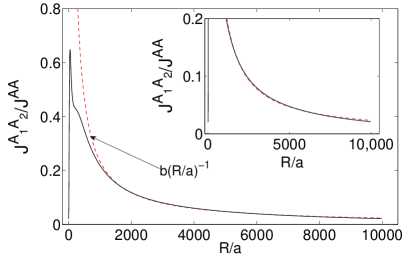
Figure 5: Plot of the $J^{A_{1}A_{2}}(\mathbf{R}_{ij})$ in units of $J^{AA}(\mathbf{R}_{ij})$ for $\mathbf{R}_{ij}$ along the armchair direction (black solid line) fitted to $\frac{b}{(R/a)}$ curve (red dashed line) as a function of $R/a$ where $b=234$.

Now we consider the $R$ dependence of the interlayer RKKY interaction between magnetic impurities located on same sublattice. Plot of $J^{A_{1}A_{2}}(\mathbf{R}_{ij})$ in units of $J^{AA}(\mathbf{R}_{ij})$ as a function of $R/a$ for $\mathbf{R}_{ij}$ along the armchair direction (Figure 1) has been shown in figure 5. Note that the oscillatory factor of $J^{A_{1}A_{2}}(\mathbf{R}_{ij})$, $1-cos[(\mathbf{K}-\mathbf{K}^{{}^{\prime}}).\mathbf{R}_{ij}+2\theta_{\mathbf{R}}]$, and that of $J^{AA}(\mathbf{R}_{ij})$, $1+cos[(\mathbf{K}-\mathbf{K}^{{}^{\prime}}).\mathbf{R}_{ij}]$, are equal for $\mathbf{R}_{ij}$ along the armchair direction. Figure 5 shows that for all impurity distances, $J^{A_{1}A_{2}}(\mathbf{R}_{ij})<J^{AA}(\mathbf{R}_{ij})$. Also we see that by increasing the impurity distance, at first $J^{A_{1}A_{2}}(\mathbf{R}_{ij})/J^{AA}(\mathbf{R}_{ij})$ increases which means that $J^{A_{1}A_{2}}(\mathbf{R}_{ij})$ decays smoother than $1/R^{3}$. Then after approaching to a maximum amount it decreases and at very large distances it shows asymptotically $1/R^{4}$ decay, which is unlike the long-distances behavior of the RKKY interaction in both SLG[18, 20, 21, 19] and ordinary 2DEG[17]. Long-distances behavior of $J^{A_{1}A_{2}}(\mathbf{R}_{ij})$ is similar to that of $J^{A_{1}B_{1}}(\mathbf{R}_{ij})$.

4.4 Magnetic impurities on different sublattices for interlayer case

We now study the interlayer RKKY interaction between magnetic impurities located on apposite sublattices. Note that two possible interlayer RKKY interactions, $J^{A_{1}B_{2}}(\mathbf{R}_{ij})$ and $J^{B_{1}A_{2}}(\mathbf{R}_{ij})$, are different and should be calculated separately. After calculating the required Green functions and substituting them into equation (9), we get following relations for $J^{A_{1}B_{2}}(\mathbf{R}_{ij})$ and $J^{B_{1}A_{2}}(\mathbf{R}_{ij})$

$$J^{A_{1}B_{2}}(\mathbf{R}_{ij})=-\frac{9g^{2}}{64\pi^{2}t}\frac{1+cos[(\mathbf{K}-\mathbf{K}^{{}^{\prime}}).\mathbf{R}_{ij}+4\theta_{\mathbf{R}}]}{(R/a)^{3}}\int_{0}^{\infty}dy[\int_{0}^{\infty}xdxJ_{2}(x)($$

$$\frac{\varepsilon_{1}}{\sqrt{x^{2}+(\frac{\gamma}{3t}\frac{R}{a})^{2}}}e^{-\varepsilon_{1}\tau}-\frac{\varepsilon_{2}}{\sqrt{x^{2}+(\frac{\gamma}{3t}\frac{R}{a})^{2}}}e^{-\varepsilon_{2}\tau})]^{2},$$ (33)

and

$$J^{B_{1}A_{2}}(\mathbf{R}_{ij})=-\frac{9g^{2}}{16\pi^{2}t}\frac{1+cos[(\mathbf{K}-\mathbf{K}^{{}^{\prime}}).\mathbf{R}_{ij}]}{(R/a)^{3}}\int_{0}^{\infty}dy[\int_{0}^{\infty}xdxJ_{0}(x)($$

$$\frac{x^{2}}{\varepsilon_{1}^{2}+x^{2}}e^{-\varepsilon_{1}\tau}-\frac{x^{2}}{\varepsilon_{2}^{2}+x^{2}}e^{-\varepsilon_{2}\tau})]^{2},$$ (34)

where $J_{2}(x)$ is Bessel function of second order. Equations (33) and (34) show that the interlayer RKKY interactions between magnetic impurities on different sublattices, $J^{A_{1}B_{2}}(\mathbf{R}_{ij})$ and $J^{B_{1}A_{2}}(\mathbf{R}_{ij})$, are always negative which indicate antiferromagnetic order. Also $J^{B_{1}A_{2}}(\mathbf{R}_{ij})$ has an anisotropic $1+cos[(\mathbf{K}-\mathbf{K}^{{}^{\prime}}).\mathbf{R}_{ij}]$ oscillatory factor which is similar to that of $J^{AA}(\mathbf{R}_{ij})$ in SLG[18, 20, 21, 19], but $J^{A_{1}B_{2}}(\mathbf{R}_{ij})$ has different oscillatory factor, $1+cos[(\mathbf{K}-\mathbf{K}^{{}^{\prime}}).\mathbf{R}_{ij}+4\theta_{\mathbf{R}}]$.

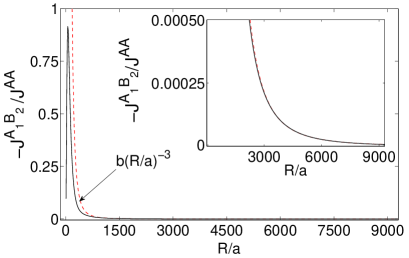
Figure 6: Plot of the $J^{A_{1}B_{2}}(\mathbf{R}_{ij})$ in units of $J^{AA}(\mathbf{R}_{ij})$ for $\mathbf{R}_{ij}$ along the armchair direction (black solid line) fitted $\frac{b}{(R/a)^{3}}$ curve (red dashed line) as a function of $R/a$ where $b=5813000$.

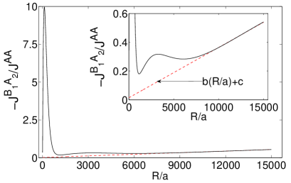
Figure 7: Plot of the $J^{B_{1}A_{2}}(\mathbf{R}_{ij})$ in units of $J^{AA}(\mathbf{R}_{ij})$ for $\mathbf{R}_{ij}$ along the armchair direction (black solid line) fitted to $b\frac{R}{a}+c$ line (red dashed line) as a function of $R/a$ where $b=0.000035$ and $c=0.0142$.

Now we consider the $R$ dependence of the interlayer RKKY interaction between magnetic impurities located on apposite sublattices. Plots of $J^{A_{1}B_{2}}(\mathbf{R}_{ij})$ and $J^{B_{1}A_{2}}(\mathbf{R}_{ij})$ in units of $J^{AA}(\mathbf{R}_{ij})$ as a function of $R/a$ for $\mathbf{R}_{ij}$ along the armchair direction have been shown in figures 6 and 7 respectively. Figure 6 shows that for small impurity distances, $J^{A_{1}B_{2}}(\mathbf{R}_{ij})$ falls off smoother than $1/R^{3}$ decay of the RKKY interaction in SLG. But by increasing impurity distance after approaching to a maximum amount, $J^{A_{1}B_{2}}(\mathbf{R}_{ij})/J^{AA}(\mathbf{R}_{ij})$ decreases which means that $J^{A_{1}B_{2}}(\mathbf{R}_{ij})$ decays faster than RKKY interaction in SLG. At large impurity distances, $J^{A_{1}B_{2}}(\mathbf{R}_{ij})$ exhibits closely $1/R^{6}$ decay which is similar to the long distances power law decay of $J^{A_{1}A_{1}}(\mathbf{R}_{ij})$ in BLG but is unlike the long distances behavior of the RKKY interaction in both SLG[18, 20, 21, 19] and ordinary 2DEG[17].

From figure 7 wee see that for small distances, by increasing $R$ first $J^{B_{1}A_{2}}(\mathbf{R}_{ij})/J^{AA}(\mathbf{R}_{ij})$ increases (which means that $J^{B_{1}A_{2}}(\mathbf{R}_{ij})$ falls of smoother than $1/R^{3}$) and after approaching to a maximum amount then it decreases (which indicates a power law decay faster than $1/R^{3}$ for $J^{B_{1}A_{2}}(\mathbf{R}_{ij})$). This behavior repeats at larger impurity distances again but with smaller maximum amount. At very large impurity distances $J^{B_{1}A_{2}}(\mathbf{R}_{ij})$ shows a decay close to $1/R^{2}$ which is similar to the long distance behavior of the RKKY interaction in the ordinary 2DEG.

As we mentioned in the subsection 4.1 , in the limit of strong interlayer coupling the low energy states are localized on $B_{1}$ and $A_{2}$ sublattices, so we only calculate and discuss the $J^{B_{1}A_{2}}(\mathbf{R}_{ij})$. In this limiting case we found

$$J^{B_{1}A_{2}}(\mathbf{R}_{ij})=-\frac{27mg^{2}a^{4}}{32\pi^{2}}\frac{1+cos[(\mathbf{K}-\mathbf{K}^{{}^{\prime}}).\mathbf{R}_{ij}]}{R^{2}}\int_{0}^{\infty}dy[\int_{0}^{\infty}xdxJ_{0}(x)e^{-x^{2}y}]^{2},$$ (35)

which after performing the integral numerically it can be written as

$$J^{B_{1}A_{2}}(\mathbf{R}_{ij})=-\frac{27mg^{2}a^{4}}{32\pi^{2}}\frac{1+cos[(\mathbf{K}-\mathbf{K}^{{}^{\prime}}).\mathbf{R}_{ij}]}{R^{2}}.$$ (36)

We see that in the strong interlayer coupling limit, the long distance behavior of the interlayer RKKY interaction in BLG is similar to that in the ordinary 2DEG but with a different $1+cos[(\mathbf{K}-\mathbf{K}^{{}^{\prime}}).\mathbf{R}_{ij}]$ oscillatory factor.

5 Summary and conclusion

In summary, we studied the intralayer and interlayer RKKY interaction between two magnetic impurities in BLG in the four-band model. We derived them semi-analytically by calculating the Green functions in the eigenvalues and eigenvectors representation. For this we first obtained the eigenvalues and eigenvectors of BLG in the four-band model and by using them the required Green functions for four possible configurations of two magnetic impurities are calculated. Then we used them to calculate corresponding intralayer and interlayer RKKY interactions.

First we summarize our results for the intralayer RKKY interaction. We found that, similar to the RKKY interaction in SLG, the intralayer RKKY interactions between magnetic impurities located on same (opposite) sublattices in BLG are always ferromagnetic (antiferromagnetic). Also the intralayer RKKY interactions in BLG have $1+cos[(\mathbf{K}-\mathbf{K}^{{}^{\prime}}).\mathbf{R}_{ij}+\theta]$ oscillatory part which is equal to that of the RKKY interaction in SLG. The phase factor $\theta$ is equal to $0$ when two magnetic impurities are on same sublattice but it is equal to $2\theta_{\mathbf{R}}$ when two magnetic impurities are on apposite sublattices. Furthermore we found that at large impurity distances, $J^{A_{1}A_{1}}(\mathbf{R}_{ij})$ falls off as $1/R^{6}$ approximately while $J^{A_{1}B_{1}}(\mathbf{R}_{ij})$ shows closely $1/R^{4}$ decay, which both power law decays are unlike $1/R^{3}$ decay of the RKKY interaction in SLG, and also unlike the $1/R^{2}$ decay of the RKKY interaction in ordinary 2DEG. But $J^{B_{1}B_{1}}(\mathbf{R}_{ij})$, similar to ordinary two dimensional electron gas, at large impurity distances decays closely as $1/R^{2}$. The other attractive result of our work is breaking symmetry of the intralayer RKKY between magnetic moments on same sublattice in BLG. In contrast to SLG which exhibits $J^{AA}(\mathbf{R}_{ij})=J^{BB}(\mathbf{R}_{ij})$ we found that $J^{B_{1}B_{1}}(\mathbf{R}_{ij})$ is always stronger than $J^{A_{1}A_{1}}(\mathbf{R}_{ij})$. This is due to the difference between the local density of states of BLG at sublattice $B_{1}$ and $A_{1}$. The tunneling between $A_{1}$ and $B_{2}$ leads to localization of low energy states on $B_{1}$ sublattices [34]. This means density of low energy states at $B_{1}$ is more than $A_{1}$ [37] and $A_{1}$ and $B_{1}$ are not equivalent. Hence $A_{1}A_{1}$ and $B_{1}B_{1}$ RKKY couplings are different (breaking symmetry of RKKY coupling between magnetic moment on same sublattices). Furthermore we found that for all impurity distances, $J^{A_{1}A_{1}}(\mathbf{R}_{ij})<J^{AA}(\mathbf{R}_{ij})$ and $J^{A_{1}B_{1}}(\mathbf{R}_{ij})<J^{AB}(\mathbf{R}_{ij})$, but for $J^{B_{1}B_{1}}(\mathbf{R}_{ij})$ we obtained $J^{B_{1}B_{1}}(\mathbf{R}_{ij})>J^{BB}(\mathbf{R}_{ij})$ for small impurity distances and $J^{B_{1}B_{1}}(\mathbf{R}_{ij})<J^{BB}(\mathbf{R}_{ij})$ for large impurity distances. It is noticeable that our results for power law decay of intralayer RKKY couplings are in agreement with what has been reported in Ref. 31.

Now we present our results for interlayer RKKY interactions in BLG. We found that, similar to the intralayer case, the interlayer RKKY interaction between magnetic impurity located on same (apposite) sublattices are also ferromagnetic (antiferromagnetic). The interlayer RKKY interactions have $1+cos[(\mathbf{K}-\mathbf{K}^{{}^{\prime}}).\mathbf{R}_{ij}+\theta]$ oscillatory factor, where $\theta$ for $J^{A_{1}A_{2}}(\mathbf{R}_{ij})$ and $J^{B_{1}B_{2}}(\mathbf{R}_{ij})$ is equal to $2\theta_{\mathbf{R}}$. But $J^{A_{1}B_{2}}(\mathbf{R}_{ij})$ and $J^{B_{1}A_{2}}(\mathbf{R}_{ij})$ have different phase factors $4\theta_{\mathbf{R}}$ and $0$ respectively. Also we found that at large distances, the interlayer RKKY interactions between magnetic located on same sublattice in BLG decay as $1/R^{4}$ approximately. But the interlayer RKKY interactions between magnetic impurities located on apposite sublattices, $J^{A_{1}B_{2}}(\mathbf{R}_{ij})$ and $J^{B_{1}A_{2}}(\mathbf{R}_{ij})$, show decays close to $1/R^{6}$ and $1/R^{2}$ decays at large impurity distances respectively. Note that only $J^{B_{1}A_{2}}(\mathbf{R}_{ij})$, similar to the RKKY interaction in ordinary 2DEG, decays as $1/R^{2}$ at large impurity distances.

To examine our results we discussed the RKKY interaction in BLG in the two limiting cases, weak $(\gamma\rightarrow 0)$ and strong $(\gamma\rightarrow\infty)$ interlayer coupling. Our results in these two limiting cases reduced to RKKY interaction in SLG and to that in BLG in the two-band approximation respectively.

References

• [1] K. S. Novosolov, A. K. Geim, S. V. Morozov, D. Jiang, Y. Zhang, S. V. Dubonos, I. V. Gregorieva and A. A. Firsov, Electric field effect in atomically thin carbon films, Science 306 (2004) 666-669.
• [2] A. H. Castro Neto, F. Guinea, N. M. R. Peres, K. S. Novoselov and A. K. Geim, The electronic properties of graphene, Rev. Mod. Phys 81 (2009) 109-162.
• [3] K. S. Novoselov, A. K. Geim, S. V. Morozov, D. Jiang, M. I. Katsnelson, I. V. Grigorieva, S. V. Dubonos and A. A. Firsov, Two-dimensional gas of massless Dirac fermions in graphene, Nature (London) 438 (2005) 197-200.
• [4] V. P. Gusynin, and S. G. Sharapov, Unconventional Integer Quantum Hall Effect in Graphene, Phys. Rev. Lett. 95 (2005) 146801:1-146801:4.
• [5] N. M. R. Peres, A. H. Castro Neto, and F. Guinea, Conductance quantization in mesoscopic graphene, Phys. Rev. B 73 (2006) 195411:1-195411:8.
• [6] J. Tworzydlo, B. Trauzettel, M. Titov, A. Rycerz, and C. W. J. Beenakker, Sub-Poissonian Shot Noise in Graphene, Phys. Rev. Lett. 96 (2006) 246802:1-246802:4.
• [7] T. Ando, Screening Effect and Impurity Scattering in Monolayer Graphene, J. Phys. Soc. Jpn. 75 (2006) 074716:1-074716:7.
• [8] M. I. Katsnelson, K. S. Novoselov, and A. K. Geim, Chiral tunnelling and the Klein paradox in graphene, Nat. Phys. 2 (2006) 620-625.
• [9] M. I. Katsnelson, Graphene: carbon in two dimensions, Mater. Today 10 (2007) 20-27.
• [10] S. V. Morozov, K. S. Novoselov, M. I. Katsnelson, F. Schedin, L. A. Ponomarenko, D. Jiang, and A. K. Geim, Strong Suppression of Weak Localization in Graphene, Phys. Rev. Lett. 97 (2006) 016801:1-016801:4.
• [11] S. Piscanec, M. Lazzeri, F. Mauri, A. C. Ferrari, and J. Robertson, Kohn Anomalies and Electron-Phonon Interactions in Graphite, Phys. Rev. Lett. 93 (2004) 185503:1-185503:4.
• [12] M. Lazzeri and F. Mauri, Nonadiabatic Kohn Anomaly in a Doped Graphene Monolayer, Phys. Rev. Lett. 97 (2006) 266407:1-266407:4.
• [13] M. A. Ruderman and C. Kittel, Indirect Exchange Coupling of Nuclear Magnetic Moments by Conduction Elecrons, Phys. Rev. 96 (1954) 99-102.
• [14] T. Kasuya, A theory of metallic ferro- and antiferromagnetism on Zener’s model, Prog. Theor. Phys. 16 (1956) 45-57.
• [15] K. Yosida, Magnetic properties of Cu-Mn alloys, Phys. Rev. 106 (1957) 893-898.
• [16] Y. Yafet, Ruderman-Kittel-Kasuya-Yosida range function of a one-dimensional free-electron gas, Phys. Rev. B 36 (1987) 3948-3949.
• [17] B. Fischer and M. W. Klein, Magnetic and nonmagnetic impurities in two-dimensional metals, Phys. Rev. B 11 (1975) 2025-2029.
• [18] S. Saremi, RKKY in half-filled bipartite lattices: Graphene as an example, Phys. Rev. B 76 (2007) 184430:1–184430:6.
• [19] A. M. Black-Schaffer, RKKY coupling in graphene, Phys. Rev. B 81 (2010) 205416:1-205416:8.
• [20] M. Sherafati and S. Satpathy, RKKY interaction in graphene from the lattice Green’s function, Phys. Rev. B 83 (2011) 165425:1–165425:8.
• [21] E. Kogan, RKKY interaction in graphene, Phys. Rev. B 84 (2011) 115119:1–115119:6.
• [22] A. M. Black-Schaffer, Importance of electron-electron interactions in the RKKY coupling in graphene, Phys. Rev. B 82 (2010) 073409:1–073409:4.
• [23] H. Lee, J. Kim, E. R. Mucciolo, G. Bouzerar, and S. Kettemann, RKKY interaction in disordered graphene, Phys. Rev. B 85 (2012) 075420:1–075420:5.
• [24] O. Roslyak, G. Gumbs and D. Huang, Gap-modulated doping effects on indirect exchange interaction between magnetic impurities in graphene, J. Appl. Phys. 113, (2013) 123702:1-123702:7.
• [25] Y. Zhang, Y. -W. Tan, H. L. Stormer and P. Kim, Experimental observation of the quantum Hall effect and Berry’s phase in graphene, Nature 438 (2005) 201-204.
• [26] E. McCann, Asymmetry gap in the electronic band structure of bilayer graphene, Phys. Rev. B(R) 74 (2006) 161403:1-161403:4.
• [27] E. V. Castro, N. M. R. Peres, J. M. B. Lopes dos Santos, A. H. Castro Neto, and F. Guinea, Localized States at Zigzag Edges of Bilayer Graphene, Phys. Rev. Lett. 100 (2008) 026802:1-026802:4.
• [28] R. V. Gorbachev, F. V. Tikhonenko, A. S. Mayorov, D. W. Horsell, and A. K. Savchenko, Weak Localization in Bilayer Graphene, Phys. Rev. Lett. 98 (2007) 176805:1-176805:4.
• [29] E. H. Hwang and S. Das Sarma, Screening, Kohn Anomaly, Friedel Oscillation, and RKKY Interaction in Bilayer Graphene, Phys. Rev. Lett. 101 (2008) 156802:1–156802:4.
• [30] X. -F. Wang, and T. Chakraborty, Coulomb screening and collective excitations in a graphene bilayer, Phys. Rev. B(R) 75 (2007) 041404:1-041404:4.
• [31] L. Jiang, X. Lu, W. Gao, G. Yu, Z. Liu and Y. Zheng, RKKY interaction in AB-sstacked multilayer graphene, J. Phys: Condens. Matter 24 (2012) 206003:-206003:12.
• [32] M. Killi, D. Heidarian, and A. Paramekanti, Controlling local moment formation and local moment interaction in bilayer graphene, New J. Phy. 13 (2011) 053043:1-053043:18.
• [33] P. Parhizgar, M. Sherafati, R. Asgari, S. Satpathy, Ruderman-Kittel-Kasuya-Yosida interaction in biased bilayer graphene, arXiv:1302.3649 (2013).
• [34] E. McCann and V. I. Fal’ko, Landau-Level Degeneracy and Quantum Hall Effect in a Graphite Bilayer, Phys. Rev. Lett. 96 (2006) 086805:1-086805:4.
• [35] A. A. Abrikosov, L. P. Gorkov, and I. E. Dzyloshinski, Methods of Quantum Field Theory in Statistical Physics, Pergamon Press, Oxford, 1965.
• [36] V. V. Cheianov, O. Syljuasen, B. L. Altshuler, and V. I. Fal’ko, Ordered states of adatoms on graphene, Phys. Rev. B 80 (2009) 233409:1-233409:4.
• [37] Z. F. Wang, Q. Li, H. Su, X. Wang, Q. W. Shi, J. Chen, J. Yang, and J. G. Hou, Electronic structure of bilayer graphene: A real-space Green’s function study, Phys. Rev. B 75 (2007) 085424:1-085424:8.
• [38] A. P. Prudnikov, Yu. A. Brychkov, and O. I. Marichev, Integrals and Series, Vol. 2, Gordon and Breach Science Publishers, Amsterdam, 1986.
• [39] The integrals in Eqs. 17 and 18 could be solved by using the mathematical identity for integral of Bessel functions[21, 38] which are $\int_{0}^{\infty}dy[\int_{0}^{\infty}xdxJ_{0}(x)e^{-xy}]^{2}=\frac{\pi}{16}$.
• [40] M. Koshino, and T. Ando, Transport in bilayer graphene: Calculations within a self-consistent Born approximation, Phys. Rev. B 73 (2006) 245403:1-245403:8.
• [41] G. N. Watson, A Treatise on the Theory of Bessel Functions, Cambridge University Press, Cambridge, 1922.
• [42] By using the mathematical identity for integral of Bessel functions[21, 41] one can show that $\int_{0}^{\infty}dy[\int_{0}^{\infty}xdxJ_{0}(x)e^{-x^{2}y}]^{2}=\frac{1}{2}$.
Refer to caption