The Renormalizable Three-Term Polynomial Inflation with Large Tensor-to-Scalar Ratio

Abstract

We systematically study the renormalizable three-term polynomial inflation in the supersymmetric and non-supersymmetric models. The supersymmetric inflaton potentials can be realized in supergravity theory, and only have two independent parameters. We show that the general renormalizable supergravity model is equivalent to one kind of our supersymmetric models. We find that the spectral index and tensor-to-scalar ratio can be consistent with the Planck and BICEP2 results, but the running of spectral index is always out of the $2\sigma$ range. If we do not consider the BICEP2 experiment, these inflationary models can be highly consistent with the Planck observations and saturate its upper bound on the tensor-to-scalar ratio ($r\leq 0.11$). Thus, our models can be tested at the future Planck and QUBIC experiments.

I Introduction

It is well-known that the standard big bang cosmology has some problems, for instance, the flatness, horizon, and monopole problems, etc, which can be solved naturally by inflation Staro ; Guth:1980zm ; Linde:1981mu ; Albrecht:1982wi . Also, the observed temperature fluctuations in the cosmic microwave background radiation (CMB) strongly suggests an accelerated expansion at a very early stage of our Universe evolution, i.e., inflation. Moreover, the inflationary models predict the cosmological perturbations in the matter density and spatial curvature from the vacuum fluctuations of the inflaton, which can explain the primordial power spectrum elegantly. Besides the scalar perturbation, the tensor perturbation is produced as well, which has special features in the B-mode of the CMB polarization data as a signature of the primordial inflation.

The Planck satellite measured the CMB temperature anisotropy with an unprecedented accuracy. From its first-year observational data Ade:2013ktc in combination with the nine years of Wilkinson Microwave Anisotropy Probe (WMAP) polarization low-multipole likelihood data Hinshaw:2012aka and the high-multipole spectra data from the Atacama Cosmology Telescope (ACT) Das:2013zf and the South Pole Telescope (SPT) Keisler:2011aw (Planck+WP+highL), the scalar spectral index $n_{s}$, the running of the scalar spectral index $n_{s}^{\prime}\equiv dn_{s}/d\ln k$, the tensor-to-scalar ratio $r$, and the scalar amplitude $A_{s}$ for the power spectrum of the curvature perturbations are respectively constrained to be Ade:2013zuv ; Ade:2013uln

$$n_{s}=0.9603\pm 0.0073~{},~{}~{}n_{s}^{\prime}=-0.0134\pm 0.0090~{},~{}~{}$$

$$r\leq 0.11~{},~{}~{}A^{1/2}_{s}=4.6856^{+0.0566}_{-0.0628}\times 10^{-5}~{}.~{}\,$$ (1)

As given by the Planck Collaboration, we also quote 68% errors on the measured parameters and 95% upper limits on the other parameters.

Recently, the BICEP2 experiment announced the discovery of the gravitational waves or primordial tensor perturbations in the B-mode power spectrum around $\ell\sim 80$ Ade:2014xna . If confirmed by future experiments, it will definitely be a huge progress in fundamental physics. The measured tensor-to-scalar ratio is

$$r~{}=~{}0.20^{+0.07}_{-0.05}~{}.~{}\,$$ (2)

Subtracting the various dust models and re-deriving the $r$ constraint still results in high significance of detection, we have

$$r~{}=~{}0.16^{+0.06}_{-0.05}~{}.~{}\,$$ (3)

Thus, the BICEP2 results are in tension with the Planck results. To be consistent with both experiments, one can consider the running of the spectral index. With it, we have the following results from the Planck+WP+highL data Ade:2013zuv

$$n_{s}=0.9570\pm 0.0075~{},~{}~{}~{}n^{\prime}_{s}=-0.022\pm 0.010~{},~{}~{}r~{}<~{}0.26~{}(95\%~{}{\rm C.L.})~{}.~{}\,$$ (4)

And the combined Planck+WP+highL+BICEP2 data give

$$n_{s}=0.9574^{+0.0073}_{-0.0074}~{},~{}~{}~{}n^{\prime}_{s}=-0.0292\pm 0.0096~{},~{}~{}r~{}=~{}0.21^{+0.05}_{-0.06}~{}.~{}\,$$ (5)

Therefore, we must at least require the running of the spectral index $n^{\prime}_{s}$ to be smaller than 0.0004 at 3$\sigma$ level for any viable inflationary model. However, there might exist the foreground subtleties in the BICEP2 experiment such as dust effects, etc. As we know, the recent observations from the Planck and BICEP2/Keck Array Collaborations provided strong constraints on the primordial tensor fluctuations Ade:2015tva ; Planck:2015xua ; Ade:2015lrj , $r<0.11$ ($r<0.12$ from BICEP2/Keck Array) at 95% Confidence Level (C.L.). Because these results were announced seven months after we submitted our paper to arXiv, we will not consider them here.

Obviously, such a large tensor-to-scalar ratio $r$ from the BICEP2 measurement does impose a strong constraint on the inflationary models. For example, most inflationary models from string theory predict small $r$ far below $0.01$ and then contradict with the BICEP2 results Burgess:2013sla . With $r=0.16$ or 0.20, we obtain that the Hubble scale during inflation is about $1.0\times 10^{14}$ GeV, and the inflaton potential is around the Grand Unified Theory (GUT) scale $2\times 10^{16}$ GeV which might have some connections with GUTs. From the naive analysis of Lyth bound Lyth:1996im , we will have large field inflation, and then the effective field theory might not be valid since the high-dimensional operators are suppressed by the reduced Planck scale. The inflationary models, which can realize $n_{s}\simeq 0.96$ and $r\simeq 0.16/0.20$, have been studied extensively Anchordoqui:2014uua ; Czerny:2014wua ; Hamada:2014iga ; Kobayashi:2014jga ; Ferrara:2014ima ; Choudhury:2014kma ; Gong:2014cqa ; Ashoorioon:2014nta ; Okada:2014lxa ; Ellis:2014rxa ; Hamaguchi:2014mza ; DiBari:2014oja ; Kawai:2014doa ; Antusch:2014cpa ; Freivogel:2014hca ; Bousso:2014jca ; Kaloper:2014zba ; Choudhury:2014wsa ; Choi:2014aca ; Murayama:2014saa ; McDonald:2014oza ; Gao:2014fha ; Gao:2014yra ; Li:2014owa ; Chialva:2014rla ; Li:2014xna ; Kallosh:2014xwa ; Gao:2014pca ; Gao:2014uha ; Nakayama:2014hga ; Choudhury:2013iaa ; Li:2014lpa ; Ben-Dayan:2014lca ; Okada:2014nia . Especially, the simple chaotic and natural inflation models are favoured.

From the particle physics point of view, supersymmetry is the most promising new physics beyond the Standard Model (SM). Especially, it can stabilize the scalar masses, and has a non-renormalized superpotential. Moreover, gravity is very important in the early Universe. Thus, a natural framework for inflationary model building is supergravity theory SUGRA . However, supersymmetry breaking scalar masses in a generic supergravity theory are of the same order as gravitino mass, giving rise to the so-called $\eta$ problem eta , where all the scalar masses are at the order of the Hubble scale due to the large vacuum energy density during inflation glv . Two elegant solutions were proposed: no-scale supergravity Cremmer:1983bf ; Ellis:1984bf ; Enqvist:1985yc ; Ellis:2013xoa ; Ellis:2013nxa ; Li:2013moa ; Ellis:2013nka , and shift symmetry in the Kähler potential Kawasaki:2000yn ; Yamaguchi:2000vm ; Yamaguchi:2001pw ; Kawasaki:2001as ; Kallosh:2010ug ; Kallosh:2010xz ; Nakayama:2013jka ; Nakayama:2013txa ; Takahashi:2013cxa ; Li:2013nfa .

The Planck satellite experiment might measure the tensor-to-scalar ratio $r$ down to 0.03-0.05 in one or two years. And the target of future QUBIC experiment is to constrain the tensor-to-scalar ratio of 0.01 at the 90% Confidence Level (C.L.) with one year of data taking from the Concordia Station at ${\rm D\hat{o}me}$ C, Antarctica Battistelli:2010aa . Thus, even if the BICEP2 results on tensor-to-scalar ratio $r$ were too large, as long as $r$ is not smaller than 0.01, for example, $r=0.05$ or $0.1$, how to construct the inflationary models which highly agree with the Planck results and have large tensor-to-scalar ratio is still a very important question since these models can be tested in the near future.

The simple inflationary models have one parameter, for example, the monomial inflaton potentials. So the next to the simple inflationary models have two parameters. In the supergravity models with two parameters, we will generically have three terms due to the square of the F-term. In particular, we show that the general renormalizable supergravity model is equivalent to one kind of our supersymmetric models. Thus, in this paper, we will classify the renormalizable three-term polynomial inflationary models for both supersymmetric and non-supersymmetric models. The supersymmetric inflaton potentials can be obtained from supergravity theory. We find that their spectral indices and tensor-to-scalar ratios can be consistent with the Planck and BICEP2 experiments. However, $n^{\prime}_{s}$ is always out of the $2\sigma$ range. In addition, even if we do not consider the BICEP2 results, we find that the three-term polynomial inflationary models can be consistent with the Planck observations. Especially, the tensor-to-scalar ratio can not only be larger than $0.01$ in the $1\sigma$ region, above the well-known Lyth bound Lyth:1996im , but also saturate the Planck upper bound $0.11$ in the $1\sigma$ region. Thus, these models produce the typical large field inflation, and can be tested at the future Planck and QUBIC experiments.

This paper is organized as follows. In Section II, we briefly review the slow-roll inflation. In Section III, we construct the supersymmetric models from the supergravity theory. In Section IV, we systematically study the three-term polynomial inflation. Our conclusion is given in Section V.

II Brief Review of Slow-Roll Inflation

In the inflation, the slow-roll parameters are defined as

$$\epsilon=\frac{M_{\rm Pl}^{2}V_{\phi}^{2}}{2V^{2}},$$ (6)

$$\eta=\frac{M_{\rm Pl}^{2}V_{\phi\phi}}{V},$$ (7)

$$\xi^{2}=\frac{M_{\rm Pl}^{4}V_{\phi}V_{\phi\phi\phi}}{V^{2}},$$ (8)

where $M^{2}_{\rm Pl}=(8\pi G)^{-1}$ is the reduced Planck scale, $V_{\phi}\equiv\partial V(\phi)/\partial\phi$, $V_{\phi\phi}\equiv\partial^{2}V(\phi)/\partial\phi^{2}$, and $V_{\phi\phi\phi}\equiv\partial^{3}V(\phi)/\partial\phi^{3}$. Also, the scalar power spectrum in the single field inflation is

$$\mathcal{P}_{\mathcal{R}}=A_{s}\left(\frac{k}{k_{*}}\right)^{n_{s}-1+n_{s}^{\prime}\ln(k/k_{*})/2},$$ (9)

where the subscript “*” means the value at the horizon crossing, the scalar amplitude is

$$A_{s}\approx\frac{1}{24\pi^{2}M^{4}_{\rm Pl}}\frac{\Lambda^{4}}{\epsilon}~{},~{}\,$$ (10)

and the scalar spectral index as well as its running at the second order are Lyth:1998xn ; Stewart:1993bc

$$\begin{split}n_{s}~{}=~{}1+2\eta-6\epsilon+2\left[\frac{1}{3}\eta^{2}+(8C-1)\epsilon\eta\right.\\ \left.-\left(\frac{5}{3}+12C\right)\epsilon^{2}-\left(C-\frac{1}{3}\right)\xi^{2}\right],\end{split}$$ (11)

$$n_{s}^{\prime}~{}=~{}16\epsilon\eta-24\epsilon^{2}-2\xi^{2},$$ (12)

where $C=-2+\ln 2+\gamma\simeq-0.73$ with $\gamma$ the Euler-Mascheroni constant. Moreover, the tensor power spectrum is

$$\mathcal{P}_{T}=A_{T}\left(\frac{k}{k_{*}}\right)^{n_{t}}~{},$$ (13)

where the tensor spectral index is Lyth:1998xn ; Stewart:1993bc

$$n_{t}=-2\epsilon\left[1+\left(4C+\frac{11}{3}\right)\epsilon-2\left(\frac{2}{3}+C\right)\eta\right]~{}.~{}$$ (14)

Thus, the tensor-to-scalar ratio is given by Lyth:1998xn ; Stewart:1993bc

$$r\equiv\frac{A_{T}}{A_{s}}=16\epsilon\left[1+8\left(C+\frac{2}{3}\right)(2\epsilon-\eta)\right]~{}.$$ (15)

Because $8(C+\frac{2}{3})\simeq-0.506667$, we can safely neglect the term $8(C+\frac{2}{3})(2\epsilon-\eta)$ at the next leading order in the above equation. Thus, we will take the next leading order approximation $r=16\epsilon$ for simplicity. Therefore, with the BICEP2 result $r=0.16/0.20$, we obtain the inflation scale about $2\times 10^{16}$ GeV and the Hubble scale around $1.0\times 10^{14}$ GeV.

The number of e-folding before the end of inflation is

$$N(\phi)~{}=~{}\int_{t_{i}}^{t_{e}}Hdt\approx\frac{1}{M_{\rm Pl}^{2}}\int_{\phi_{e}}^{\phi_{i}}\frac{V(\phi)}{V_{\phi}(\phi)}d\phi=\frac{1}{\sqrt{2}\,M_{\rm Pl}}\int_{\phi_{e}}^{\phi_{i}}\frac{d\phi}{\sqrt{\epsilon(\phi)}},$$ (16)

where the value $\phi_{i}$ of the inflaton at the beginning of the inflation is the value at the horizon crossing, and the value $\phi_{e}$ of the inflaton at the end of inflation is defined by either $\epsilon(\phi_{e})=1$ or $\eta(\phi_{e})=1$. From the above equation, we get the Lyth bound Lyth:1996im

$$\Delta\phi\equiv|\phi_{i}-\phi_{e}|>{\sqrt{2\epsilon_{\rm min}}}N(\phi)M_{\rm Pl}~{},~{}\,$$ (17)

where $\epsilon_{\rm min}$ is the minimal $\epsilon$ during inflation. If $\epsilon(\phi)$ is a monotonic function of $\phi$, we have $\epsilon_{\rm min}=\epsilon(\phi_{i})\equiv\epsilon$. Thus, for $r=0.01$, 0.05, 0.1, 0.16, and 0.21, we obtain the large field inflation due to $\Delta\phi>1.77~{}M_{\rm Pl}$, $4.0~{}M_{\rm Pl}$, $5.6~{}M_{\rm Pl}$, $7.1~{}M_{\rm Pl}$, and $8.1~{}M_{\rm Pl}$ for $N(\phi)=50$, respectively. Moreover, to violate the Lyth bound and have the magnitude of $\phi$ smaller than the reduced Planck scale during inflation, we require that $\epsilon(\phi)$ be not a monotonic function and have a minimum between $\phi_{i}$ and $\phi_{e}$.

In this paper, we will consider the renormalizable three-term polynomial inflation with large tensor-to-scalar ratio. With slow-roll condition, each term in the polynomial potential will be around $10^{-8}M^{4}_{\rm Pl}$ or smaller. However, without slow-roll condition and with fine-tuning, each term could be much larger than $10^{-8}M^{4}_{\rm Pl}$ and there exist large cancellations among three terms. Thus, the quantum corrections can be very large and then out of control during large field inflation.

III Supergravity Model Building

In this paper, to simplify the discussions, we take $M_{\rm Pl}=1$. In the non-supersymmetric inflationary models, we will consider the following polynomial potentials at the renormalizable level

$$V = a_{0}+a_{1}\phi+a_{2}\phi^{2}+a_{3}\phi^{3}+a_{4}\phi^{4}~{},~{}$$ (18)

where $\phi$ is the inflaton, and $a_{i}$ are couplings. In the supersymmetric inflationary models from the supergravity theory, there are some relations among $a_{i}$. Before we construct the concrete models, let us briefly review the supergravity model building.

In the supergravity theory with a Kähler potential $K$ and a superpotential $W$, the scalar potential is

$$V=e^{K}\left((K^{-1})^{i}_{\bar{j}}D_{i}WD^{\bar{j}}\overline{W}-3|W|^{2}\right)~{},~{}$$ (19)

where $(K^{-1})^{i}_{\bar{j}}$ is the inverse of the Kähler metric $K_{i}^{\bar{j}}=\partial^{2}K/\partial\Phi^{i}\partial{\bar{\Phi}}_{\bar{j}}$, and $D_{i}W=W_{i}+K_{i}W$. Moreover, the kinetic term for a scalar field is

$${\cal L}~{}=~{}K_{i}^{\bar{j}}\partial_{\mu}\Phi^{i}\partial^{\mu}{\bar{\Phi}}_{\bar{j}}~{}.~{}\,$$ (20)

We first briefly review the generic model building. Introducing two superfields $\Phi$ and $X$, we consider the Kähler potential and superpotential as below

$$K=-\frac{1}{2}(\Phi-{\bar{\Phi}})^{2}+X{\bar{X}}-\delta(X{\bar{X}})^{2}~{},~{}$$ (21)

$$W~{}=~{}Xf(\Phi)~{}.~{}\,$$ (22)

Thus, the above Kähler potential $K$ is invariant under the following shift symmetry Kawasaki:2000yn ; Yamaguchi:2000vm ; Yamaguchi:2001pw ; Kawasaki:2001as ; Kallosh:2010ug ; Kallosh:2010xz ; Nakayama:2013jka ; Nakayama:2013txa ; Takahashi:2013cxa ; Li:2013nfa

$$\Phi\rightarrow\Phi+CM_{\rm Pl}~{},~{}\,$$ (23)

with $C$ a dimensionless real parameter. In general, the Kähler potential $K$ is a function of $\Phi-{\bar{\Phi}}$ and independent on the real part of $\Phi$. Before further discussions, we shall present a few comments on the Kähler potential and superpotential

• If shift symmetry is a global symmetry, it will be violated by quantum gravity effects, i.e., one might add high-dimensional operators suppressed by the reduced Planck scale. To solve this problem, one can consider gauged discrete symmetry from anomalous $U(1)_{X}$ gauge symmetry inspired from string models, and then quantum gravity violating effects can be forbidden.

• Shift symmetry is violated by the superpotential in Eq. (25). In principle, we can break the shift symmetry spontaneuously by introducing a spurion field $S$ and extending the shift symmetry as follows Kawasaki:2000ws

  $$\Phi\rightarrow\Phi+CM_{\rm Pl}~{},~{}~{}S\rightarrow\frac{S\Phi}{\Phi+CM_{\rm Pl}}\,~{}.~{}$$ (24)

  And we consider the following superpotential

  $$W~{}=~{}Xf(S\Phi/M_{\rm Pl})~{},~{}\,$$ (25)

  which is clearly invariant under the extended shift symmetry. After $S$ obtains a non-zero vacuum expectation values, we obtain the superpotential in Eq. (25). The effects from spontaneous shift symmetry breaking have been studied in Ref. Mazumdar:2014bna .

• In a supersymmetric theory, the superpotential is non-renormalized, while there indeed exist quantum corrections to the Kähler potential in general. In the renormalizable three-term polynomial inflation which we shall study in the following, the inflaton value is about $10M_{\rm Pl}$, and each term in the scalar potential is about $10^{-8}M^{4}_{\rm Pl}$ or smaller during inflation. The Kähler potential for $\Phi$ in Eq. (21) is about $100M^{2}_{\rm Pl}$, and the quantum corrections will be around $10^{-6}M^{2}_{\rm Pl}$ from the naive dimensional annalyses with loop factor. Thus, such quantum corrections are under control and negligible.

  In addition, supersymmetry is violated during inflation. Thus, the masses for the scalar and fermionic components of any superfield may be splitted. And then we might have additional one-loop effective scalar potential, which may affect the inflation and is beyond the scope of our current paper.

From the above Kähler potential and superpotential, the scalar potential is given by

$$V = e^{K}\left[|(\Phi-{\bar{\Phi}})Xf(\Phi)+X\frac{\partial f(\Phi)}{\partial\Phi}|^{2}+|({\bar{X}}-2\delta X{\bar{X}}^{2})Xf(\Phi)+f(\Phi)|^{2}\right.$$ (26)

$$\left.-3|Xf(\Phi)|^{2}\right]~{}.~{}\,$$

Because there is no real component ${\rm Re}[\Phi]$ of $\Phi$ in the Kähler potential due to the shift symmetry, this scalar potential along ${\rm Re}[\Phi]$ is very flat and then ${\rm Re}[\Phi]$ is a natural inflaton candidate. From the previous studies Kallosh:2010ug ; Kallosh:2010xz ; Li:2013nfa , we can stabilize the imaginary component ${\rm Im}[\Phi]$ of $\Phi$ and $X$ at the origin during inflation, i.e., ${\rm Im}[\Phi]=0$ and $X=0$. Therefore, with ${\rm Re}[\Phi]=\phi/{\sqrt{2}}$, we get the inflaton potential

$$V~{}=~{}|f(\phi/{\sqrt{2}})|^{2}~{}.~{}\,$$ (27)

For a renormalizable superpotential, we have

$$f(\Phi)~{}=~{}a^{\prime}_{0}+a^{\prime}_{1}{\sqrt{2}}\Phi+2a^{\prime}_{2}\Phi^{2}~{},~{}\,$$ (28)

where we choose $a_{i}$ as real numbers. And then the polynomial inflaton potential is

$$V = |a^{\prime}_{0}+a^{\prime}_{1}\phi+a^{\prime}_{2}\phi^{2}|^{2}~{}.~{}\,$$ (29)

The polynomial inflations from supergravity model building have been considered before. At the renormalizable level, only the case with $a_{1}^{\prime}\not=0$ and $a_{2}^{\prime}\not=0$ has been studied in the literatures Kallosh:2014xwa ; Nakayama:2013jka ; Nakayama:2013txa . In this paper, we also consider the following three cases with $a_{0}^{\prime}\not=0$: (1) $a_{0}^{\prime}\not=0$ and $a_{1}^{\prime}\not=0$; (2) $a_{0}^{\prime}\not=0$ and $a_{2}^{\prime}\not=0$; (3) The most general case with $a_{0}^{\prime}\not=0$, $a_{1}^{\prime}\not=0$, and $a_{2}^{\prime}\not=0$. Moreover, we study the three-term polynomial inflations whose coefficients for the lowest and highest order terms in the inflaton potential can be negative. These inflations cannot be realized in supergravity model building where the coefficients for the lowest and highest order terms must be positive.

IV The Renormalizable Three-Term Polynomial Inflation

To classify the three-term polynomial inflation at renormalizable level, we consider the following inflaton potential

$$V = a_{j}\phi^{j}+a_{k}\phi^{k}+a_{l}\phi^{l}~{},~{}$$ (30)

where $0\leq j<k<l\leq 4$. With $(j,~{}k,~{}l)$, we will study all the renormalizable non-supersymmetric and supersymmetric three-term polynomial inflation with large tensor-to-scalar ratio $r$, which can be consistent with the Planck and/or BICEP2 experiments. For simplicity, we denote the maximum and minimum of the inflaton potential as $\phi_{M}$ and $\phi_{m}$, respectively. Because we shall consider the super-Planckian inflation, our inflation around the maxima and minima of inflaton potentials is similar to the inflection point inflation Allahverdi:2006iq ; Allahverdi:2006we ; Allahverdi:2008bt ; Enqvist:2010vd .

IV.1 Inflaton Potential with $(j,~{}k,~{}l)=(0,~{}1,~{}2)$

First, we consider the non-supersymmetric models with the inflaton potential $V=a_{0}+a_{1}\phi+a_{2}\phi^{2}$. For $a_{2}<0$, there exists a maximum at $\phi_{M}=-\frac{a_{1}}{2a_{2}}$. No matter the slow-roll inflation occurs at the right or left of this maximum (which is the same because of symmetry), we cannot find any $r$ within the $2\sigma$ range of the BICEP2 data. And the numerical results for $r$ versus $n_{s}$ is given in Fig. 1. When $n_{s}$ is within the $1\sigma$ range $0.9603\pm 0.0073$, the range of $r$ is $[0.0132,~{}0.0534]$.

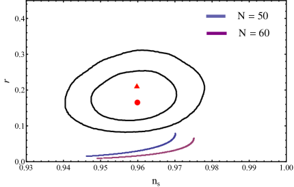
Figure 1: $r$ versus $n_{s}$ for the inflaton potential with $(j,~{}k,~{}l)=(0,~{}1,~{}2)$ and $a_{2}<0$. The inner and outer circles are $1\sigma$ and $2\sigma$ regions, respectively.

Moreover, for $a_{2}>0$ and $a_{1}<0$, we have a minimum at $\phi_{m}=-\frac{a_{1}}{2a_{2}}$. We present the numerical results for $r$ versus $n_{s}$ in Fig. 2, where the inner and outer circles are $1\sigma$ and $2\sigma$ regions, respectively. For $n_{s}$ in the $1\sigma$ range $0.9603\pm 0.0073$, the range of $r$ is $[0.0132,~{}0.16160]$, which can be consistent with the BICEP2 experiment. In addition, for the number of e-folding $N_{e}=50$, $n_{s}$ and $r$ are within $1\sigma$ and $2\sigma$ regions of the BICEP2 experiment for $a_{1}>-30a_{2}$ and $a_{0}<\frac{a_{1}^{2}+2a_{2}^{2}}{4a_{2}}$ and for $a_{1}>-10a_{2}$ and $a_{0}<\frac{a_{1}^{2}+2a_{2}^{2}}{4a_{2}}$, respectively. Also, for $N_{e}=60$, $n_{s}$ and $r$ are within $2\sigma$ region for $a_{1}>-10a_{2}$ and $a_{0}<\frac{a_{1}^{2}+2a_{2}^{2}}{4a_{2}}$, but no viable parameter space for $1\sigma$ region. In particular, the best fit point with $n_{s}=0.96$ and $r=0.16$ for the BICEP2 data can be obtained for $N_{e}=50$, $a_{2}\approx-a_{1}$ and $a_{2}\approx-3a_{0}$. For example, $a_{0}=3,~{}a_{1}=-10$, and $a_{2}=10$, and the corresponding $\phi_{i},~{}\phi_{e}$, and $\phi_{m}$ respectively are $-13.621,~{}0.464$, and $0.5$. Thus, we obtain $\Delta\phi=14.085$, which satisfies the Lyth bound. In the following discussions, we will not comment on $\Delta\phi$ since the Lyth bound is always satisfied in our models.

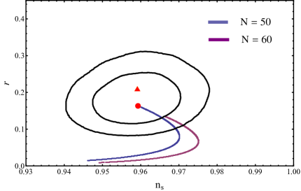
Figure 2: $r$ versus $n_{s}$ for the inflaton potential with $(j,~{}k,~{}l)=(0,~{}1,~{}2)$, $a_{1}<0$, and $a_{2}>0$.

Second, we consider the supersymmetric model with inflaton potential $V=a^{2}+2ab\phi+b^{2}\phi^{2}$, which has a minimum at $-a/b$. We obtain that for $\phi=-a/b\pm\sqrt{2}$, both $\epsilon$ and $\eta$ are equal to 1, and then the slow-roll inflation ends. Also, we find that no matter the slow-roll inflation occurs at the left or right of the minimum, $n_{s}$ and $r$ can be written as functions of the e-folding number $N_{e}$

$$n_{s}~{}=~{}1-\frac{8}{4N_{e}+2}~{},~{}~{}~{}r~{}=~{}\frac{32}{4N_{e}+2}$$ (31)

Thus, for $N_{e}=50$, we get $n_{s}=0.9604$ and $r=0.1584$. And for $N_{e}=60$, we get $n_{s}=0.9669$ and $r=0.1322$. In fact, this is similar to the chaotic inflation with inflaton potential $\phi^{2}$.

IV.2 Inflaton Potential with $(j,~{}k,~{}l)=(0,~{}1,~{}3)$

The inflaton potential is $V=a_{0}+a_{1}\phi+a_{3}\phi^{3}$. First, we consider $a_{1}>0$ and $a_{3}<0$. Because there is a minimum at $\phi_{m}=-\sqrt{-\frac{a_{1}}{3a_{3}}}$ and a maximum at $\phi_{M}=\sqrt{-\frac{a_{1}}{3a_{3}}}$, we have three inflationary trajectories, and let us discuss them one by one. When the slow-roll inflation occurs at the left of the minimum, the numerical results for $r$ versus $n_{s}$ is given in Fig. 3. The range of $r$ is about $[0.1231,~{}0.2237]$ for $n_{s}$ within its $1\sigma$ range $0.9603\pm 0.0073$, which is consistent with the BICEP2 results. In the viable parameter space, we generically have $a_{0}<a_{1}$. For the number of e-folding $N_{e}=50$, $n_{s}$ and $r$ are within $1\sigma$ and $2\sigma$ regions of the BICEP2 experiment for $-11a_{3}<a_{1}<-1000a_{3}$ and $-11a_{3}<a_{1}<-5000a_{3}$, respectively. For the number of e-folding $N_{e}=60$, $n_{s}$ and $r$ are within $1\sigma$ and $2\sigma$ regions of the BICEP2 experiment for $a_{1}<-125a_{3}$ and $a_{1}<-600a_{3}$, respectively. To be concrete, we will present two best fit points for the BICEP2 data. The best fit point with $n_{s}=0.963$ and $r=0.16$ can be realized for $N_{e}=50$, $a_{0}\thickapprox a_{1}\thickapprox-230a_{3}$, for example, $a_{0}=1,a_{1}=1$ and $a_{3}=-0.00436$, and the corresponding $\phi_{i},~{}\phi_{f},~{}\phi_{m}$, and $\phi_{M}$ are respectively $-27.1459,-15.3793,-8.74372$, and $8.74372$. Another best fit point with $n_{s}=0.959$ and $r=0.196$ can be obtained for $N_{e}=60$, $a_{0}\thickapprox a_{1}\thickapprox-2a_{3}$, for example, $a_{0}=1,~{}a_{1}=1$, and $a_{3}=-0.5$, and the corresponding $\phi_{i},~{}\phi_{f},~{}\phi_{m}$, and $\phi_{M}$ are $-19.2289,~{}-2.35496,~{}-0.816497$, and $0.816497$, respectively. In addition, when slow-roll inflation occurs at the right of the minimum, we also present the numerical results for $r$ versus $n_{s}$ in Fig. 3. The range of $r$ is about [0.0337, 0.0669] for $n_{s}$ within its $1\sigma$ range $0.9603\pm 0.0073$. Although we can not fit the BICEP2 data, we still have large enough tensor-to-scalar ratio, which can be tested at the future Planck and QUBIT experiments.

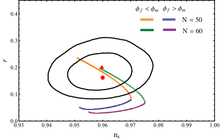
Figure 3: $r$ versus $n_{s}$ for the inflaton potential with $(j,~{}k,~{}l)=(0,~{}1,~{}3)$, $a_{1}>0$, and $a_{3}<0$, where the inflationary trajectories are at the left and right of the minimum.

Furthermore, for the slow-roll inflation at the right of the maximum, the numerical results for $r$ versus $n_{s}$ is given in Fig. 4. For $n_{s}$ in the $1\sigma$ range $0.9603\pm 0.0073$, the range of $r$ is $[0.0085,~{}0.0482]$, which is within the reach of the future Planck and QUBIT experiments.

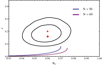
Figure 4: $r$ versus $n_{s}$ for the inflaton potential with $(j,~{}k,~{}l)=(0,~{}1,~{}3)$, $a_{1}>0$, and $a_{3}<0$, where the inflationary trajectory is at the right of the maximum.

Second, we consider $a_{1}<0$ and $a_{3}<0$, the potential will decrease monotonically, and the curves for $r$ versus $n_{s}$ are given in Fig. 5. The range of $r$ is about $[0.1670,~{}0.2427]$ for $n_{s}$ within its $1\sigma$ range $0.9603\pm 0.0073$, which is consistent with the BICEP2 results. In the viable parameter space, we generically have $a_{0}\thickapprox 1$. For the number of e-folding $N_{e}=50$, $n_{s}$ and $r$ are within $1\sigma$ and $2\sigma$ regions of the BICEP2 experiment for $-90a_{3}<-a_{1}<-300a_{3}$ and $-a_{1}<-1000a_{3}$, respectively. For the number of e-folding $N_{e}=60$, $n_{s}$ and $r$ are within $1\sigma$ and $2\sigma$ regions of the BICEP2 experiment for $-a_{1}<-210a_{3}$ and $-a_{1}<-300a_{3}$, respectively. The best fit point with $n_{s}=0.96$ and $r=0.206$ can be realized for $N_{e}=60$, $a_{0}\thickapprox 1$ and $-a_{1}\thickapprox-90a_{3}$, for example, $a_{0}=1,a_{1}=-90$ and $a_{3}=-1$, and the corresponding $\phi_{i}$ and $\phi_{f}$ are respectively $-15.2061$ and $-0.7038$.

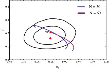
Figure 5: $r$ versus $n_{s}$ for the inflaton potential with $(j,~{}k,~{}l)=(0,~{}1,~{}3)$, $a_{1}<0$, and $a_{3}<0$.

IV.3 Inflaton Potential with $(j,~{}k,~{}l)=(0,~{}1,~{}4)$

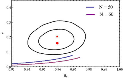
Figure 6: $r$ versus $n_{s}$ for the inflaton potential with $(j,~{}k,~{}l)=(0,~{}1,~{}4)$, $a_{1}>0$, and $a_{4}<0$ for inflation at the left of the maximum.

We consider the non-supersymmetric inflation models with $V=a_{0}+a_{1}\phi+a_{4}\phi^{4}$. First, we consider $a_{1}>0$ and $a_{4}<0$. There is a maximum at $\phi_{M}=\left(-\frac{a_{1}}{4a_{4}}\right)^{1/3}$. When slow-roll inflation occurs at the left and right of the maximum, we present the numerical results for $r$ versus $n_{s}$ in Figs. 6 and 7, respectively. For $n_{s}$ in the $1\sigma$ range $0.9603\pm 0.0073$, the corresponding ranges of $r$ are $[0.0250,~{}0.0732]$ and $[0.0077,~{}0.0459]$, respectively, which is large enough to be tested at the future Planck and QUBIT experiments.

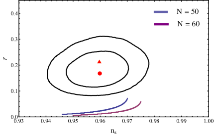
Figure 7: $r$ versus $n_{s}$ for the inflaton potential with $(j,~{}k,~{}l)=(0,~{}1,~{}4)$, $a_{1}>0$, and $a_{4}<0$ for inflation at the right of the maximum.

Second, we consider $a_{1}<0$ and $a_{4}>0$. There exists a minimum at $\phi_{m}=\left(-\frac{a_{1}}{4a_{4}}\right)^{1/3}$. If the slow-roll inflation occurs at the left of the minimum, we obtain $n_{s}\leq 0.94$ and $r>0.3$, which is not consistent with the Planck and BICEP2 data. When the slow-roll inflation occurs at the right of the minimum, the numerical results for $r$ versus $n_{s}$ is given in Fig. 8. With $n_{s}$ in the $1\sigma$ range $0.9603\pm 0.0073$, the range of $r$ is about $[0.1288,~{}0.2498]$, which agrees with the BICEP2 experiment. Moreover, for the number of e-folding $N_{e}=50$, $n_{s}$ and $r$ are within $1\sigma$ and $2\sigma$ regions of the BICEP2 experiment for $-5\times 10^{4}a_{4}<a_{1}<-1000a_{4}$ and $-1\times 10^{6}a_{4}<a_{1}<-3000a_{4}$, respectively. And for $N_{e}=60$, $n_{s}$ and $r$ are within $1\sigma$ and $2\sigma$ regions of the BICEP2 experiment for $-1\times 10^{4}a_{4}<a_{1}<-100a_{4}$ and $-5\times 10^{4}a_{4}<a_{1}$, respectively. To be concrete, we will present the best fit point for the BICEP2 data. The best fit point with $n_{s}=0.9607$ and $r=0.2035$ can be realized for $N_{e}=60$, $a_{1}<-100a_{0}$, and $a_{1}\thickapprox-1000a_{4}$, for example, $a_{0}=1,~{}a_{1}=-1000$, and $a_{4}=1$, and the corresponding $\phi_{i},~{}\phi_{f}$, and $\phi_{m}$ are respectively $26.1887,~{}10.8134$, and $6.29961$.

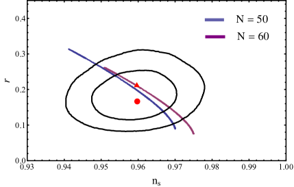
Figure 8: $r$ versus $n_{s}$ for the inflaton potential with $(j,~{}k,~{}l)=(0,~{}1,~{}4)$, $a_{1}<0$, and $a_{4}>0$.

IV.4 Inflaton Potential with $(j,~{}k,~{}l)=(0,~{}2,~{}3)$

We consider the inflationary model with potential $V=a_{0}+a_{2}\phi^{2}+a_{3}\phi^{3}$. First, for $a_{2}>0$ and $a_{3}<0$, there exist a minimum at $\phi_{m}=0$ and a maximum at $\phi_{M}=-\frac{2a_{2}}{3a_{3}}$. So we have three inflationary trajectories, and let us discuss them one by one. When the slow-roll inflation occurs at the left of the minimum, we present the numerical results for $r$ versus $n_{s}$ in Fig. 9. For $n_{s}$ within its $1\sigma$ range $0.9603\pm 0.0073$, the range of $r$ is about $[0.1363,~{}0.2206]$, which agree with the BICEP2 results. For the number of e-folding $N_{e}=50$, $n_{s}$ and $r$ are within $1\sigma$ and $2\sigma$ regions of the BICEP2 experiment for $a_{2}>-5a_{3}$ and $a_{0}<{\rm Max}(a_{2}/2,-2a_{3})$ and for $a_{0}<{\rm Max}(a_{2}/2,-2a_{3})$, respectively. Also, for $N_{e}=60$, $n_{s}$ and $r$ are within $1\sigma$ and $2\sigma$ regions of the BICEP2 experiment for $a_{0}<{\rm Max}(a_{2}/2,-2a_{3})$. To be concrete, we will present two best fit points for the BICEP2 data. The best fit point with $n_{s}=0.96$ and $r=0.16$ can be realized for $N_{e}=50$, $a_{2}>10a_{0}$ and $a_{2}\thickapprox 10^{3}a_{3}$, for instance, $a_{0}=1,~{}a_{2}=10$, and $a_{3}=-0.01$, and the corresponding $\phi_{i},~{}\phi_{f}$, and $\phi_{m}$ are respectively $-14.2222,~{}-1.34067$, and $0$. Another best fit point with $n_{s}=0.958$ and $r=0.199$ can be obtained for $N_{e}=59$, $a_{2}\approx 40a_{0}$, and $a_{2}\thickapprox-2a_{3}$, for example, $a_{0}=1,a_{2}=10$ and $a_{3}=-0.01$, and the corresponding $\phi_{i},~{}\phi_{f}$, and $\phi_{m}$ are respectively $-18.3869,~{}-1.73496$, and $0$.

In addition, when slow-roll inflation occurs at the right of the minimum, the numerical results for $r$ versus $n_{s}$ are given in Fig. 9 as well. The range of $r$ is about $[0.0645,~{}0.160]$ for $n_{s}$ within its $1\sigma$ range $0.9603\pm 0.0073$. In the viable parameter space, we have $a_{0}<a_{2}/2$ in general. For the number of e-folding $N_{e}=50$, $n_{s}$ and $r$ are within $1\sigma$ and $2\sigma$ regions of the BICEP2 experiment for $a_{2}>-50a_{3}$ and $a_{2}>-30a_{3}$, respectively. And for the number of e-folding $N_{e}=60$, $n_{s}$ and $r$ are out of the $1\sigma$ region of the BICEP2 experiment and are within $2\sigma$ region for $a_{2}>-50a_{3}$. The best fit point with $n_{s}=0.96$ and $r=0.158$ for the BICEP2 data can be realized for $N_{e}=50$, $a_{2}>10a_{0}$, and $a_{2}>-10^{4}a_{3}$, for instance, $a_{0}=0.1,~{}a_{2}=1$, and $a_{3}=-10^{-4}$, and the corresponding $\phi_{i},~{}\phi_{f},~{}\phi_{m}$, and $\phi_{M}$ are respectively $14.1854,~{}1.33945,~{}0.0$, and $6666.67$.

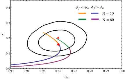
Figure 9: $r$ versus $n_{s}$ for the inflaton potential with $(j,~{}k,~{}l)=(0,~{}2,~{}3)$ where the inflationary trajectories are at the left and right of the minimum.

Furthermore, for the slow-roll inflation at the right of the maximum, the numerical results for $r$ versus $n_{s}$ are given in Fig. 10. For $n_{s}$ in the $1\sigma$ range $0.9603\pm 0.0073$, the range of $r$ is $[0.0097,~{}0.0431]$, which can be tested at the future Planck and QUBIT experiments.

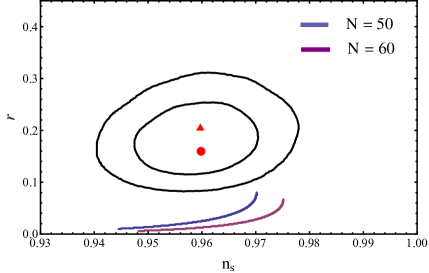
Figure 10: $r$ versus $n_{s}$ for the inflaton potential with $(j,~{}k,~{}l)=(0,~{}2,~{}3)$ where the inflationary trajectory is at the right of the maximum.

Second, for $a_{2}<0$ and $a_{3}<0$, there exist a minimum at $\phi_{m}=-\frac{2a_{2}}{3a_{3}}$ and a maximum at $\phi_{M}=0$. Similar to the above discussions, there exist three inflationary trajectories, and we will discuss them one by one. When the slow-roll inflation occurs at the left of the minimum, we present the numerical results for $r$ versus $n_{s}$ in Fig. 11. For $n_{s}$ within its $1\sigma$ range $0.9603\pm 0.0073$, the range of $r$ is about $[0.1249,~{}0.2242]$, which can be consistent with the BICEP2 experiment. Generically, we have $a_{0}\thickapprox 1$. For the number of e-folding $N_{e}=50$, $n_{s}$ and $r$ are within $1\sigma$ and $2\sigma$ regions of the BICEP2 experiment for $-a_{2}<-30a_{3}$ and $-a_{2}<-100a_{3}$, respectively. Also, for $N_{e}=60$, $n_{s}$ and $r$ are within $1\sigma$ and $2\sigma$ regions of the BICEP2 experiment respectively for $-a_{2}<-15a_{3}$ and $-a_{2}<-35a_{3}$. To be concrete, we will present two best fit points for the BICEP2 data. The best fit point with $n_{s}=0.959$ and $r=0.196$ can be realized for $N_{e}=60$, $a_{0}=1$, and $-a_{2}\thickapprox-2a_{3}$, for instance, $a_{0}=1,~{}a_{2}=-2$, and $a_{3}=-1$, and the corresponding $\phi_{i},~{}\phi_{f}$, and $\phi_{m}$ are respectively $-19.8863,~{}-3.10761$, and $-1.33333$.

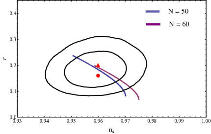
Figure 11: $r$ versus $n_{s}$ for the inflaton potential with $(j,~{}k,~{}l)=(0,~{}2,~{}3)$ where the inflationary trajectory is at the left of the minimum.

In addition, when the slow-roll inflations occur at the right of the minimum and maximum, we present the numerical results for $r$ versus $n_{s}$ in Figs. 12 and 13. For $n_{s}$ within its $1\sigma$ range $0.9603\pm 0.0073$, the corresponding ranges of $r$ are respectively $[0.0104,~{}0.0512]$ and $[0.0099,~{}0.0505]$, which are within the reach of the future Planck and BICEP2 experiments.

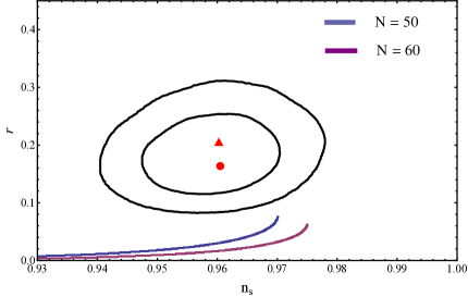
Figure 12: $r$ versus $n_{s}$ for the inflaton potential with $(j,~{}k,~{}l)=(0,~{}2,~{}3)$ where the inflationary trajectory is at the right of the minimum.

Figure 13: $r$ versus $n_{s}$ for the inflaton potential with $(j,~{}k,~{}l)=(0,~{}2,~{}3)$ where the inflationary trajectory is at the right of the maximum.

Third, for $a_{2}<0$ and $a_{3}>0$, there exist a maximum at $\phi_{M}=0$ and a minimum at $\phi_{m}=-\frac{2a_{2}}{3a_{3}}$. Similarly, we have three inflationary trajectories, and will discuss them one by one as well. When the slow-roll inflations occur at the left and right of the maximum, we present the numerical results for $r$ versus $n_{s}$ in Figs. 14 and 15, respectively. For $n_{s}$ within its $1\sigma$ range $0.9603\pm 0.0073$, the corresponding ranges of $r$ are $[0.0099,~{}0.0485]$ and $[0.0097,~{}0.0515]$, which can be tested at the future Planck and BICEP2 experiments.

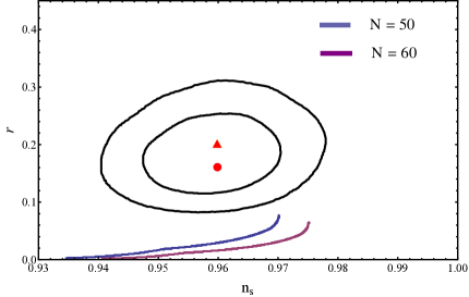
Figure 14: $r$ versus $n_{s}$ for the inflaton potential with $(j,~{}k,~{}l)=(0,~{}2,~{}3)$ where the inflationary trajectory is at the left of the maximum.

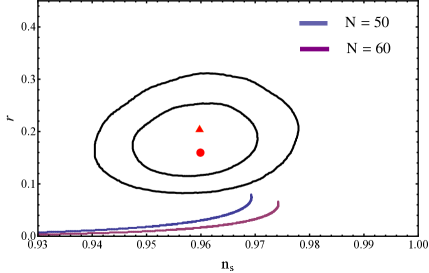
Figure 15: $r$ versus $n_{s}$ for the inflaton potential with $(j,~{}k,~{}l)=(0,~{}2,~{}3)$ where the inflationary trajectory is at the right of the maximum.

Furthermore, for the slow-roll inflation at the right of the minimum, the numerical results for $r$ versus $n_{s}$ are given in Fig. 16. For $n_{s}$ in the $1\sigma$ range $0.9603\pm 0.0073$, the range of $r$ is $[0.1232,~{}0.2253]$, which can be consistent with the BICEP2 experiment. In general, we can take $a_{0}\thickapprox 1$. For the number of e-folding $N_{e}=50$, $n_{s}$ and $r$ are within $1\sigma$ and $2\sigma$ regions of the BICEP2 experiment for $-a_{2}<30a_{3}$ and $-a_{2}<100a_{3}$ respectively. Also, for $N_{e}=60$, $n_{s}$ and $r$ are within $1\sigma$ and $2\sigma$ regions of the BICEP2 experiment respectively for $-a_{2}<15a_{3}$ and $-a_{2}<35a_{3}$. The best fit point with $n_{s}=0.959$ and $r=0.196$ can be realized for $N_{e}=60$, $a_{0}=1$ and $-a_{2}\thickapprox-2a_{3}$, for instance, $a_{0}=1,~{}a_{2}=-2$, and $a_{3}=1$, and the corresponding $\phi_{i},~{}\phi_{f}$, and $\phi_{m}$ are respectively $19.8863,~{}3.10761$, and $1.33333$.

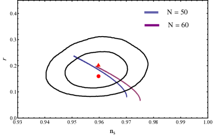
Figure 16: $r$ versus $n_{s}$ for the inflaton potential with $(j,~{}k,~{}l)=(0,~{}2,~{}3)$ where the inflationary trajectory is at the right of the minimum.

IV.5 Inflaton Potential with $(j,~{}k,~{}l)=(0,~{}2,~{}4)$

First, we consider the non-supersymmetric inflation models with potential $V=a_{0}+a_{2}\phi^{2}+a_{4}\phi^{4}$. For simplicity, we only study the hill-top scenario with $a_{0}>0$, $a_{2}>0$, and $a_{4}<0$. Thus, there is a maximum at $\phi=\phi_{M}=\sqrt{-\frac{a_{2}}{2a_{4}}}$. For the slow-roll inflation occurs at the left of the maximum with $0<\phi_{f}<\phi_{i}<\phi_{M}$, to achieve a proper $r$, we require $|a_{4}|\ll a_{2}$ to get a relatively large $\phi_{M}$, and thus, the $\phi^{2}$ term dominates the potential. We present the numerical results for $r$ versus $n_{s}$ in Fig. 17. For $n_{s}$ in the $1\sigma$ range $0.9603\pm 0.0073$, the range of $r$ is $[0.0480,~{}0.1565]$, which can be consistent with the BICEP2 experiment. In the viable parameter space, we always have $a_{2}>10a_{0}$. Moreover, for the number of e-folding $N_{e}=50$, $n_{s}$ and $r$ are within $1\sigma$ and $2\sigma$ regions of the BICEP2 experiment for $a_{2}>-1000a_{4}$ and $a_{2}>-700a_{4}$, respectively. Also, for $N_{e}=60$, $n_{s}$ and $r$ are within $2\sigma$ region for $a_{2}>-1200a_{4}$, but no viable parameter space for $1\sigma$ region. The best fit point with $n_{s}=0.96$ and $r=0.158$ for the BICEP2 data can be obtained for $N_{e}=50$, $a_{2}>10^{5}a_{4}$, and $a_{2}>10a_{0}$. For example, $a_{0}=1$, $a_{2}=10$, and $a_{4}=-10^{-4}$, and the corresponding $\phi_{i}$, $\phi_{f}$, and $\phi_{M}$ are respectively $14.1817,1.33953$, and $223.607$.

Figure 17: $r$ versus $n_{s}$ for the non-supersymmetric inflaton potential with $(j,~{}k,~{}l)=(0,~{}2,~{}4)$, $a_{0}>0$, $a_{2}>0$, and $a_{4}<0$, where the inflationary trajectory is at the left of the maximum.

In addition, when slow-roll inflation occurs at the right of the maximum, i.e., $\phi_{M}<\phi_{i}<\phi_{f}$, the numerical results for $r$ versus $n_{s}$ are given in Fig. 18. For $n_{s}$ within its $1\sigma$ range $0.9603\pm 0.0073$, the range of $r$ is about $[0.0072,~{}0.0444]$, which is within the reach of the future Planck and QUBIT experiments.

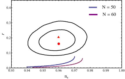
Figure 18: $r$ versus $n_{s}$ for the non-supersymmetric inflaton potential with $(j,~{}k,~{}l)=(0,~{}2,~{}4)$, $a_{0}>0$, $a_{2}>0$, and $a_{4}<0$, where the inflationary trajectory is at the right of the maximum.

Second, we consider the supersymmetric inflationary model with potential $V=|a+b\phi^{2}|^{2}=a^{2}+2ab\phi^{2}+b^{2}\phi^{4}$. For simplicity, we assume $a>0$ and $b<0$. So the potential has two minima at $\phi=\phi_{m}=\pm\sqrt{-\frac{a}{b}}$. Without loss of generality, we only consider the positive branch of the filed $\phi=\phi_{m}=\sqrt{-\frac{a}{b}}$. The inflationary process can occur at either the left or right of the minimum. When the slow-roll inflation occurs at the left of the minimum, i.e., $\phi_{i}<\phi_{f}<\phi_{m}$, we present the numerical results for $r$ versus $n_{s}$ in Fig. 19. For $n_{s}$ in its $1\sigma$ range $0.9603\pm 0.0073$, the range of $r$ is $[0.0254,~{}0.1585]$. In addition, for the number of e-folding $N_{e}=50$, $n_{s}$ and $r$ are within $1\sigma$ and $2\sigma$ regions of the BICEP2 experiment for $a>-1650b$ and $a>-550b$, respectively. Also, for $N_{e}=60$, $n_{s}$ and $r$ are within $2\sigma$ region for $a>-1650b$, but no viable parameter space for $1\sigma$ region. Also, the best fit point with $n_{s}=0.96$ and $r=0.158$ for the BICEP2 data can be obtained for $N_{e}=50$ and $a>-3\times 10^{7}b$. For example, $a=1$ and $b=-3\times 10^{-7}$, and the corresponding $\phi_{i},~{}\phi_{e}$, and $\phi_{m}$ are respectively $3148.08,~{}3160.86$, and $3162.28$.

Furthermore, when the slow-roll inflation occurs at the right of the minimum, i.e., $\phi_{m}<\phi_{f}<\phi_{i}$, the numerical results for $r$ versus $n_{s}$ are given in Fig. 19. Interestingly, we will always get a larger $r$ than the above case for any value of $a$ or $b$. With $n_{s}$ in its $1\sigma$ range $0.9603\pm 0.0073$, the range of $r$ is about $[0.1319,~{}0.2484]$. In addition, for the number of e-folding $N_{e}=50$, $n_{s}$ and $r$ are within $1\sigma$ and $2\sigma$ regions of the BICEP2 experiment for $a>-165b$ and $a>-33b$, respectively. Also, for $N_{e}=60$, $n_{s}$ and $r$ are within $1\sigma$ region for $a>-17b$, and $2\sigma$ region for the viable parameter space. Let us present two best fit points for the BICEP2 data. The best fit point with $n_{s}=0.96$ and $r=0.16$ can be realized for $N_{e}=50$ and $a\thickapprox-1\times 10^{6}b$. For example, $a=1$ and $b=-1\times 10^{-6}$, and the corresponding $\phi_{i},~{}\phi_{f}$, and $\phi_{m}$ are respectively $1014.25,~{}1001.42$, and $1000.0$. Another best fit point with $n_{s}=0.96$ and $r=0.2$ can be obtained for $a=165$ and $b=-1$. For example, $a=165$ and $b=-1$, and the corresponding $\phi_{i},~{}\phi_{f}$, and $\phi_{m}$ are $30.5877$, $14.3371$, and $12.8452$, respectively.

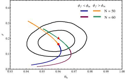
Figure 19: $r$ versus $n_{s}$ for the supersymmetric inflaton potential with $(j,~{}k,~{}l)=(0,~{}2,~{}4)$.

IV.6 Inflaton Potential with $(j,~{}k,~{}l)=(0,~{}3,~{}4)$

We consider the inflaton potential $V=a_{0}+a_{3}\phi^{3}+a_{4}\phi^{4}$. First, we study the hill-top scenario with $a_{0}>0$, $a_{3}>0$, and $a_{4}<0$. So there is a maximum at $\phi_{M}=-\frac{3a_{3}}{4a_{4}}$. When the slow-roll inflation occurs at the left of the maximum, i.e., $\phi_{f}<\phi_{i}<\phi_{M}$, we present the numerical results for $r$ versus $n_{s}$ in Fig. 20. The range of $r$ is about $[0.0742,~{}0.1956]$ for $n_{s}$ within its $1\sigma$ range $0.9603\pm 0.0073$, which can be consistent with the BICEP2 results. In the viable parameter space, we generically have $a_{0}<a_{3}$. For the number of e-folding $N_{e}=50$, $n_{s}$ and $r$ are within $1\sigma$ and $2\sigma$ regions of the BICEP2 experiment for $a_{3}>-33a_{4}$ and $a_{3}>-26a_{4}$, respectively. And for $N_{e}=60$, $n_{s}$ and $r$ are within $1\sigma$ and $2\sigma$ regions of the BICEP2 experiment for $a_{3}>-40a_{4}$ and $a_{3}>-29a_{4}$, respectively. Let us present two best fit points for the BICEP2 data. The best fit point with $n_{s}=0.96$ and $r=0.16$ can be realized for $N_{e}=59$, $a_{3}>10a_{0}$, and $a_{3}\thickapprox-58.4a_{4}$, for example, $a_{0}=10,~{}a_{3}=100$, and $a_{4}=-1.71$, and the corresponding $\phi_{i},~{}\phi_{f}$, and $\phi_{M}$ are respectively $18.0429,~{}2.07119$, and $43.8596$. Another best fit point with $n_{s}=0.959$ and $r=0.196$ can be obtained for $N_{e}=60$, $a_{3}\approx 5a_{0}$, and $a_{3}\thickapprox-1000a_{4}$, for instance, $a_{0}=20,a_{3}=100$, and $a_{4}=-0.1$, and the corresponding $\phi_{i},~{}\phi_{f}$, and $\phi_{M}$ are $19.0411,~{}2.07322$, and $750.0$, respectively.

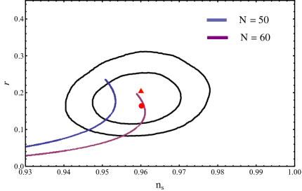
Figure 20: $r$ versus $n_{s}$ for the inflaton potential with $(j,~{}k,~{}l)=(0,~{}3,~{}4)$ where the inflationary trajectory is at the left of the maximum.

Moreover, we consider the slow-roll inflation occurs at the right of the maximum, i.e., $\phi_{M}<\phi_{i}<\phi_{f}$. The numerical results for $r$ versus $n_{s}$ is given in Fig. 21. For $n_{s}$ within the $1\sigma$ range $0.9603\pm 0.0073$, the range of $r$ is $[0.0067,~{}0.0454]$, which is large enough to be tested at the future Planck and QUBIT experiments.

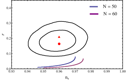
Figure 21: $r$ versus $n_{s}$ for the inflaton potential with $(j,~{}k,~{}l)=(0,~{}3,~{}4)$ where the inflationary trajectory is at the right of the maximum.

Second, we consider the other case with $a_{0}>0$, $a_{3}<0$, and $a_{4}>0$, which has a minimum at $\phi_{m}=-\frac{3a_{3}}{4a_{4}}$. When the slow-roll inflation occurs at the left of the minimum, i.e., $\phi_{i}<\phi_{f}<\phi_{m}$, we present the numerical results for $r$ versus $n_{s}$ in Fig. 22. The range of $r$ is about $[0.1995,~{}0.2473]$ for $n_{s}$ within its $1\sigma$ range $0.9603\pm 0.0073$, which can be consistent with the BICEP2 results. In the viable parameter space, we generically have $a_{0}\thickapprox 1$. For the number of e-folding $N_{e}=50$, $n_{s}$ and $r$ are within $2\sigma$ region of the BICEP2 experiment for $-a_{3}>50a_{4}$ but no viable parameter space for $1\sigma$ region. And for $N_{e}=60$, $n_{s}$ and $r$ are within $1\sigma$ region of the BICEP2 experiment for $-a_{3}>15a_{4}$, and will always lie in $2\sigma$ region for any values of $a_{3}$ and $a_{4}$. The best fit point with $n_{s}=0.958$ and $r=0.199$ can be realized for $N_{e}=60$, $a_{0}\thickapprox 1$, and $a_{3}\thickapprox-1000a_{4}$, for example, $a_{0}=1,~{}a_{3}=-1000$, and $a_{4}=1$, and the corresponding $\phi_{i},~{}\phi_{f}$, and $\phi_{m}$ are respectively $-19.1319,~{}-2.1226$, and $750$.

In addition, let us consider the slow-roll inflation, which occurs at the right of the minimum, i.e., $\phi_{m}<\phi_{f}<\phi_{i}$. We present the numerical results for $r$ versus $n_{s}$ in Fig. 23. The range of $r$ is about $[0.1311,~{}0.2512]$ for $n_{s}$ within its $1\sigma$ range $0.9603\pm 0.0073$, which can be consistent with the BICEP2 results. In the viable parameter space, we have $a_{0}\thickapprox 1$ in general. For the number of e-folding $N_{e}=50$, $n_{s}$ and $r$ are within $1\sigma$ and $2\sigma$ regions of the BICEP2 experiment for $10a_{4}<-a_{3}<150a_{4}$ and $15a_{4}<-a_{3}<60a_{4}$, respectively. And for $N_{e}=60$, $n_{s}$ and $r$ are within $1\sigma$ and $2\sigma$ regions of the BICEP2 experiment for $-a_{3}<55a_{4}$ and $8a_{4}<-a_{3}<32a_{4}$, respectively. The best fit point with $n_{s}=0.96$ and $r=0.2$ can be obtained for $N_{e}=54$, $a_{0}=1$, and $-a_{3}\thickapprox-19a_{4}$, for instance, $a_{0}=1,a_{3}=-19$, and $a_{4}=1$, and the corresponding $\phi_{i},~{}\phi_{f}$, and $\phi_{m}$ are $33.5051,~{}19.7918$, and $14.25$, respectively.

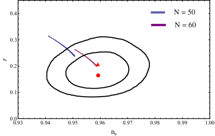
Figure 22: $r$ versus $n_{s}$ for the inflaton potential with $(j,~{}k,~{}l)=(0,~{}3,~{}4)$ and $a_{3}<0$, where the inflationary trajectory is at the left of the minimum.

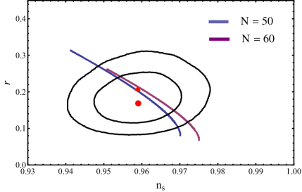
Figure 23: $r$ versus $n_{s}$ for the inflaton potential with $(j,~{}k,~{}l)=(0,~{}3,~{}4)$ and $a_{3}<0$, where the inflationary trajectory is at the right of the minimum.

IV.7 Inflaton Potential with $(j,~{}k,~{}l)=(1,~{}2,~{}3)$

We consider the inflaton potential $V=a_{1}\phi+a_{2}\phi^{2}+a_{3}\phi^{3}$. For simplicity, we only study the hill-top scenario with $a_{1}>0$, $a_{2}>0$, and $a_{3}<0$. So, there exist a minimum at $\phi_{m}=-\frac{a_{2}}{3a_{3}}-\frac{1}{3}\sqrt{\frac{a_{2}^{2}-3a_{1}a_{3}}{a_{3}^{2}}}$ and a maximum at $\phi_{M}=-\frac{a_{2}}{3a_{3}}+\frac{1}{3}\sqrt{\frac{a_{2}^{2}-3a_{1}a_{3}}{a_{3}^{2}}}$. We find that only the inflationary processes near the minimum will give us a proper $r$. First, for the slow-roll inflation at the left of the minimum, we present the numerical results for $r$ versus $n_{s}$ in Fig. 24. With $n_{s}$ in its $1\sigma$ range $0.9603\pm 0.0073$, the range of $r$ is about $[0.1234,0.2207]$, which can be consistent with the BICEP2 results. Moreover, for the number of e-folding $N_{e}=50$, $n_{s}$ and $r$ are within $1\sigma$ and $2\sigma$ regions of the BICEP2 experiment for $-20a_{3}<a_{1}<-1000a_{3}$ and $a_{1}<1000~{}{\rm Max}(a_{2},-a_{3})$, respectively. Also, for $N_{e}=60$, $n_{s}$ and $r$ are within $1\sigma$ and $2\sigma$ regions for $a_{1}<-100a_{3}$ and $a_{1}<-1000a_{3}$, respectively. Let us present two best fit points for the BICEP2 data. The best fit point with $n_{s}=0.963$ and $r=0.16$ can be realized for $N_{e}=50$, $a_{2}>10a_{1}$, and $a_{2}\thickapprox-10^{3}a_{3}$, for example, $a_{1}=0.1,~{}a_{2}=1$, and $a_{3}=-10^{-3}$, and the corresponding $\phi_{i},~{}\phi_{f},~{}\phi_{m}$, and $\phi_{M}$ are respectively $-14.2966,~{}-1.46697,~{}-0.0499963$, and $666.717$. Another best fit point with $n_{s}=0.958$ and $r=0.2$ can be obtained for $N_{e}=58$, $a_{2}>10a_{1}$, and $a_{2}\thickapprox-3.3a_{3}$, for example, $a_{1}=0.1,a_{2}=1$ and $a_{3}=-0.3$, and the corresponding $\phi_{i},~{}\phi_{f},~{}\phi_{m}$, and $\phi_{M}$ are $-17.9616,~{}-1.64821,~{}-0.0000499989$, and 2.22227, respectively.

Second, we consider the slow-roll inflation at the right of the minimum. The numerical results for $r$ versus $n_{s}$ are given in Fig. 24 as well. The range of $r$ is about $[0.0337,~{}0.158]$ for $n_{s}$ in its $1\sigma$ range $0.9603\pm 0.0073$, which can be consistent with the BICEP2 results. In addition, for the number of e-folding $N_{e}=50$, $n_{s}$ and $r$ are within $1\sigma$ and $2\sigma$ regions of the BICEP2 experiment for $a_{2}>-50a_{3}$ and $a_{1}<a_{2}(1+\ln{-\frac{a_{2}}{50a_{3}}})$ and for $a_{2}>-32a_{3}$ and $a_{1}<8[a_{2}(1+\ln{-\frac{a_{2}}{32a_{3}}})]$, respectively. Also, for $N_{e}=60$, $n_{s}$ and $r$ are within $2\sigma$ region for $a_{2}>-50a_{3}$ and $a_{1}<2[a_{2}(1+\ln{-\frac{a_{2}}{50a_{3}}})]$, but no viable parameter space for $1\sigma$ region. Especially, the best fit point with $n_{s}=0.96$ and $r=0.158$ for the BICEP2 data can be obtained for $N_{e}=50$, $a_{2}>10a_{1}$, and $a_{2}>-10^{4}a_{3}$. For example, $a_{1}=0.1,~{}a_{2}=1$, and $a_{3}=-10^{-4}$, and the corresponding $\phi_{i},~{}\phi_{f},~{}\phi_{m}$, and $\phi_{M}$ respectively are $14.1599,~{}1.36588,~{}-0.0499996$, and $6666.72$.

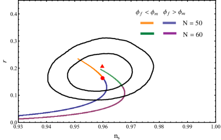
Figure 24: $r$ versus $n_{s}$ for the inflaton potential with $(j,~{}k,~{}l)=(1,~{}2,~{}3)$ where the inflationary trajectories are at the left and right of the minimum.

Third, for the slow-roll inflation at the right of the maximum, we present the numerical results for $r$ versus $n_{s}$ in Fig. 25. So we cannot find the proper parameter space which can give a large enough $r$ in the $2\sigma$ region of the BICEP2 data. For $n_{s}$ within the $1\sigma$ range $0.9603\pm 0.0073$, the range of $r$ is $[0.0083,~{}0.0471]$, which can still be tested at the future Planck and QUBIT experiments.

Figure 25: $r$ versus $n_{s}$ for the inflaton potential with $(j,~{}k,~{}l)=(1,~{}2,~{}3)$ where the inflationary trajectory is at the right of the maximum.

IV.8 Inflaton Potential with $(j,~{}k,~{}l)=(1,~{}2,~{}4)$

For the inflaton potential $V=a_{1}\phi+a_{2}\phi^{2}+a_{4}\phi^{4}$, we consider the hill-top scenario with $a_{4}<0$. Thus, either we have only one maximum at

$$\phi_{m}=\frac{\left(1-i\sqrt{3}\right)a_{2}}{2\sqrt[3]{3}\sqrt[3]{\sqrt{3}\sqrt{27a_{1}^{2}a_{4}^{4}+8a_{2}^{3}a_{4}^{3}}-9a_{1}a_{4}^{2}}}-\frac{\left(1+i\sqrt{3}\right)\sqrt[3]{\sqrt{3}\sqrt{27a_{1}^{2}a_{4}^{4}+8a_{2}^{3}a_{4}^{3}}-9a_{1}a_{4}^{2}}}{4\ 3^{2/3}a_{4}}~{},$$ (32)

or we have one minimum given by the above Eq. (32) and two maxima at

$$\phi_{M1}=\frac{1}{2}\left(\frac{\sqrt[3]{\sqrt{3}\sqrt{27a_{1}^{2}a_{4}^{4}+8a_{2}^{3}a_{4}^{3}}-9a_{1}a_{4}^{2}}}{3^{2/3}a_{4}}-\frac{2a_{2}}{\sqrt[3]{3}\sqrt[3]{\sqrt{3}\sqrt{27a_{1}^{2}a_{4}^{4}+8a_{2}^{3}a_{4}^{3}}-9a_{1}a_{4}^{2}}}\right)~{},$$ (33)

and

$$\phi_{M2}=\frac{\left(1+i\sqrt{3}\right)a_{2}}{2\sqrt[3]{3}\sqrt[3]{\sqrt{3}\sqrt{27a_{1}^{2}a_{4}^{4}+8a_{2}^{3}a_{4}^{3}}-9a_{1}a_{4}^{2}}}-\frac{\left(1-i\sqrt{3}\right)\sqrt[3]{\sqrt{3}\sqrt{27a_{1}^{2}a_{4}^{4}+8a_{2}^{3}a_{4}^{3}}-9a_{1}a_{4}^{2}}}{4\ 3^{2/3}a_{4}}~{},~{}\,$$ (34)

with $\phi_{M1}<\phi_{M2}$. For the former case with $\phi_{m}$ as a maximum, because the parameters can only be considered in a very restricted way, we cannot get a proper $r$. Therefore, we will consider the later case with $\phi_{m}$ a minimum.

First, we consider the inflation at the left of the maximum, i.e., $\phi_{f}<\phi_{i}<\phi_{M1}$. We present the numerical results for $r$ versus $n_{s}$ in Fig. 26. So we cannot find the viable parameter space which can generate a large enough $r$. For $n_{s}$ in the $1\sigma$ range $0.9603\pm 0.0073$, the range of $r$ is $[0.0084,~{}0.0449]$. Interestingly, such $r$ can still be within the reach of the future Planck and QUBIT experiments.

Figure 26: $r$ versus $n_{s}$ for the inflaton potential with $(j,~{}k,~{}l)=(1,~{}2,~{}4)$ where the inflationary trajectory is at the left of the maximum $\phi_{M1}$.

Second, we consider the inflationary trajectory between $\phi_{M1}$ and $\phi_{m}$, i.e., $\phi_{M1}<\phi_{i}<\phi_{f}<\phi_{m}$. We present the numerical results for $r$ versus $n_{s}$ in Fig. 27. For $n_{s}$ within the $1\sigma$ range $0.9603\pm 0.0073$, the range of $r$ is $[0.0487,~{}0.1585]$, which can be consistent with the BICEP2 experiment. In addition, for the number of e-folding $N_{e}=50$, $n_{s}$ and $r$ are within $1\sigma$ and $2\sigma$ regions of the BICEP2 experiment for $a_{2}>-1250a_{4}$ and $a_{1}<[a_{2}(1+20\ln{\frac{a_{2}}{-1250a_{4}}})]/10$ and for $a_{2}>-660a_{4}$ and $a_{1}<[a_{2}(1+20\ln{\frac{a_{2}}{-660a_{4}}})]/10$, respectively. Also, for $N_{e}=60$, $n_{s}$ and $r$ are within $2\sigma$ region for $a_{2}>-1100a_{4}$ and $a_{1}<[a_{2}(1+20\ln{\frac{a_{2}}{-1100a_{4}}})]/10$, but no viable parameter space for $1\sigma$ region. The best fit point with $n_{s}=0.96$ and $r=0.158$ for the BICEP2 data can be obtained for $N_{e}=50$, $a_{2}>10a_{1}$, and $a_{2}>-10^{6}a_{4}$. For example, $a_{1}=0.1,~{}a_{2}=1$, and $a_{4}=-10^{-6}$, and the corresponding $\phi_{i},~{}\phi_{f},~{}\phi_{M1}$, and $\phi_{m}$ are respectively $-14.2625,~{}-1.46598,~{}-707.082$, and $-0.05$.

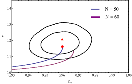
Figure 27: $r$ versus $n_{s}$ for the inflaton potential with $(j,~{}k,~{}l)=(1,~{}2,~{}4)$ where the inflationary trajectory is between $\phi_{M1}$ and $\phi_{m}$.

Third, we consider the inflationary trajectory between $\phi_{m}$ and $\phi_{M2}$, i.e., $\phi_{m}<\phi_{f}<\phi_{i}<\phi_{M2}$. We present the numerical results for $r$ versus $n_{s}$ in Fig. 28. For $n_{s}$ in the $1\sigma$ range $0.9603\pm 0.0073$, the range of $r$ is $[0.0487,~{}0.1585]$. This case is similar to the above second case with $\phi_{M1}<\phi_{i}<\phi_{f}<\phi_{m}$, so we will not present benchmark point here.

Figure 28: $r$ versus $n_{s}$ for the inflaton potential with $(j,~{}k,~{}l)=(1,~{}2,~{}4)$ where the inflationary trajectory is between $\phi_{m}$ and $\phi_{M2}$.

Fourth, we consider the inflation at the right of the maximum $\phi_{M2}$, i.e., $\phi_{M2}<\phi_{i}<\phi_{f}$. The numerical results for $r$ versus $n_{s}$ are given in Fig. 29. With $n_{s}$ in its $1\sigma$ range $0.9603\pm 0.0073$, the range of $r$ is about $[0.0084,~{}0.0449]$. Similar to the first case, $r$ is not large enough, but can still be tested at the future Planck and QUBIT experiments.

Figure 29: $r$ versus $n_{s}$ for the inflaton potential with $(j,~{}k,~{}l)=(1,~{}2,~{}4)$ where the inflationary trajectory is at the right of the maximum $\phi_{M2}$.

IV.9 Inflaton Potential with $(j,~{}k,~{}l)=(1,~{}3,~{}4)$

We consider the inflaton potential $V=a_{1}\phi+a_{3}\phi^{3}+a_{4}\phi^{4}$. For simplicity, we focus on the hill-top scenario with $a_{1}>0$ and $a_{3}>0$ while $a_{4}<0$. So, there exists a maximum as follows

$$\phi=\phi_{M}=\frac{1}{4}\left(\frac{a_{3}^{2}}{a_{4}\sqrt[3]{-a_{3}^{3}-8a_{1}a_{4}^{2}+4\sqrt{4a_{1}^{2}a_{4}^{4}+a_{1}a_{3}^{3}a_{4}^{2}}}}-\frac{a_{3}}{a_{4}}+\frac{\sqrt[3]{-a_{3}^{3}-8a_{1}a_{4}^{2}+4\sqrt{4a_{1}^{2}a_{4}^{4}+a_{1}a_{3}^{3}a_{4}^{2}}}}{a_{4}}\right)~{}.$$ (35)

First, for the inflation at the left of the maximum with $\phi_{f}<\phi_{i}<\phi_{M}$, we present the numerical results for $r$ versus $n_{s}$ in Fig. 30. For $n_{s}$ within the $1\sigma$ range $0.9603\pm 0.0073$, the range of $r$ is $[0.0556,~{}0.2328]$, which can be consistent with the BICEP2 experiment. In addition, for the number of e-folding $N_{e}=50$, $n_{s}$ and $r$ are within $1\sigma$ and $2\sigma$ regions of the BICEP2 experiment for $a_{3}>-30a_{4}$ and $100a_{3}<a_{1}<100\left[3\tan{\left(\sec^{-1}{\left(-a_{3}/10a_{4}+3\right)}-2.5\right)}+7\right]a_{3}$ and for $a_{3}>-25a_{4}$ and $a_{1}<100\left[3\tan{\left(\sec^{-1}{\left(-a_{3}/10a_{4}+0.8\right)}-2.5\right)}+13\right]a_{3}$ , respectively. Also, for $N_{e}=60$, $n_{s}$ and $r$ are within $1\sigma$ and $2\sigma$ regions for $a_{3}>-35a_{4}$ and $a_{1}<100\left[3\tan{\left(\sec^{-1}{\left(-a_{3}/10a_{4}+6.5\right)}-2.5\right)}+6\right]a_{3}$ and for $a_{3}>-30a_{4}$ and $a_{1}<100\left[3\tan{\left(\sec^{-1}{\left(-a_{3}/10a_{4}+1.7\right)}-2.5\right)}+8\right]a_{3}$, respectively. Let us present two best fit points for the BICEP2 data. The best fit point with $n_{s}=0.96$ and $r=0.16$ can be realized for $N_{e}=50$, $a_{1}\thickapprox 100a_{3}$, and $a_{3}\thickapprox-36.5a_{4}$, for example, $a_{1}=10000,a_{3}=100$, and $a_{4}=-2.74$, and the corresponding $\phi_{i},~{}\phi_{f}$, and $\phi_{M}$ are respectively $12.3513,~{}0.714071$, and $28.4959$. Another best fit point with $n_{s}=0.96$ and $r=0.2$ can be obtained for $N_{e}=60$, $a_{1}\thickapprox 90a_{3}$, and $a_{3}\thickapprox-1000a_{4}$, for example, $a_{1}=9000,~{}a_{3}=100$, and $a_{4}=-0.1$, and the corresponding $\phi_{i},~{}\phi_{f}$, and $\phi_{M}$ are $15.1757,~{}0.715088$, and $750.04$, respectively.

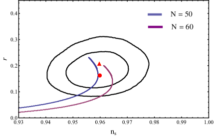
Figure 30: $r$ versus $n_{s}$ for the inflaton potential with $(j,~{}k,~{}l)=(1,~{}3,~{}4)$ where the inflationary trajectory is at the left of the maximum.

Second, we consider the inflation at the right of the maximum with $\phi_{M}<\phi_{f}<\phi_{i}$, we present the numerical results for $r$ versus $n_{s}$ in Fig. 31. For $n_{s}$ within the $1\sigma$ range $0.9603\pm 0.0073$, the range of $r$ is $[0.0081,~{}0.0458]$, which is still within the reach of the future Planck and QUBIT experiments.

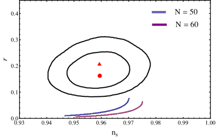
Figure 31: $r$ versus $n_{s}$ for the inflaton potential with $(j,~{}k,~{}l)=(1,~{}3,~{}4)$ where the inflationary trajectory is at the right of the maximum.

IV.10 Inflaton Potential with $(j,~{}k,~{}l)=(2,~{}3,~{}4)$

First, we consider the non-supersymmetric models with inflaton potential $V=a_{2}\phi^{2}+a_{3}\phi^{3}+a_{4}\phi^{4}$. For simplicity, we assume $a_{2}>0$ and $a_{3}>0$, while $a_{4}<0$. Thus, there exist a minimum at $\phi_{m}=0$ as well as two maxima at $\phi_{M1}=\frac{-3a_{3}-\sqrt{9a_{3}^{2}-32a_{2}a_{4}}}{8a_{4}}$ and $\phi_{M2}=\frac{-3a_{3}+\sqrt{9a_{3}^{2}-32a_{2}a_{4}}}{8a_{4}}$. Thus, we shall discuss four cases as follows:

(1) When the slow-roll inflation occurs at the left of the maximum $\phi_{M1}$, i.e., $\phi_{f}<\phi_{i}<\phi_{M1}$, $a_{2}$ must be large enough to get a $\phi_{f}$ with a relatively large absolute value, and we present the numerical results for $r$ versus $n_{s}$ in Fig. 32. For $n_{s}$ in the $1\sigma$ range $0.9603\pm 0.0073$, the range of $r$ is $[0.0073,~{}0.0472]$, which is out of the $2\sigma$ region for the BICEP2 data. Interestingly, we still have large enough tensor-to-scalar ratio within the reach of the future Planck and QUBIT experiments.

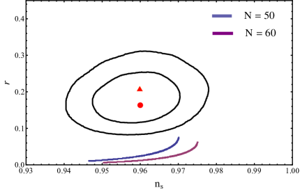
Figure 32: $r$ versus $n_{s}$ for the non-supersymmetric inflaton potential with $(j,~{}k,~{}l)=(2,~{}3,~{}4)$ where the inflationary trajectory is at the left of the maximum $\phi_{M1}$.

(2) For the slow-roll inflation occurs at the right of $\phi_{M1}$, i.e., $\phi_{M1}<\phi_{i}<\phi_{f}<\phi_{m}$, we can obtain large $r$ via chaotic inflation by requiring $a_{3}\ll a_{2}$ and $a_{4}\ll a_{2}$. The numerical results for $r$ versus $n_{s}$ are given in Fig. 33. With $n_{s}$ in the $1\sigma$ range $0.9603\pm 0.0073$, the range of $r$ is $[0.0496,~{}0.1585]$, which can be consistent with the BICEP2 experiment. In the viable parameter space, we generically have $a_{2}>1000a_{3}$. Moreover, for the number of e-folding $N_{e}=50$, $n_{s}$ and $r$ are within $1\sigma$ and $2\sigma$ regions of the BICEP2 experiment for $a_{2}>-1250a_{4}$ and $a_{2}>-660a_{4}$, respectively. Also, for $N_{e}=60$, $n_{s}$ and $r$ are within $2\sigma$ region for $a_{2}>-1000a_{4}$, but no viable parameter space for $1\sigma$ region. The best fit point with $n_{s}=0.96$ and $r=0.158$ for the BICEP2 data can be obtained for $N_{e}=50$, $a_{2}>10^{4}a_{3}$, and $a_{2}>-10^{6}a_{4}$. For instance, $a_{2}=10000,~{}a_{3}=1$, and $a_{4}=-0.01$, and the corresponding $\phi_{i},~{}\phi_{e}$, and $\phi_{M1}$ are respectively $-14.2086,~{}-1.41411$, and $-670.6$.

Figure 33: $r$ versus $n_{s}$ for the non-supersymmetric inflaton potential with $(j,~{}k,~{}l)=(2,~{}3,~{}4)$ where the inflationary trajectory is at the right of the maximum $\phi_{M1}$.

(3) When the slow-roll inflation occurs at the left of the maximum $\phi_{M2}$, i.e., $\phi_{m}<\phi_{f}<\phi_{i}<\phi_{M2}$, we present the numerical results for $r$ versus $n_{s}$ in Fig. 34. For $n_{s}$ in the $1\sigma$ range $0.9603\pm 0.0073$, the range of $r$ is $[0.0490,~{}0.2228]$, which can be consistent with the BICEP2 experiment. For the number of e-folding $N_{e}=50$, $n_{s}$ and $r$ are within $1\sigma$ and $2\sigma$ regions of the BICEP2 experiment for $a_{2}>-1000a_{4}$ and $a_{3}>-150a_{4}$ and for $a_{2}>-660a_{4}$ and $a_{3}>-100a_{4}$, respectively. For the number of e-folding $N_{e}=60$, $n_{s}$ and $r$ are within $1\sigma$ and $2\sigma$ regions of the BICEP2 experiment for $a_{2}>-1550a_{4}$ and $a_{3}>-150a_{4}$ and for $a_{2}>-1250a_{4}$ and $a_{3}>-100a_{4}$, respectively. Let us give two best fit points for the BICEP2 data. The best fit point with $n_{s}=0.96$ and $r=0.16$ can be realized for $N_{e}=50$, $a_{2}\approx 900a_{3}$, and $a_{3}>-10^{3}a_{4}$, for example, $a_{2}=90,~{}a_{3}=0.1$, and $a_{4}=-0.0001$, and the corresponding $\phi_{i},~{}\phi_{f}$, and $\phi_{M2}$ are respectively $14.249,~{}1.41532$, and $1143.52$. Another best fit point with $n_{s}=0.959$ and $r=0.1953$ can be obtained for $N_{e}=60$, $a_{2}\approx a_{3}$, and $a_{3}\approx-10^{3}a_{4}$, for instance, $a_{2}=1,~{}a_{3}=1$, and $a_{4}=-0.001$, and the corresponding $\phi_{i},~{}\phi_{f}$, and $\phi_{M2}$ are $18.7512,~{}1.87413$, and $750.666$, respectively.

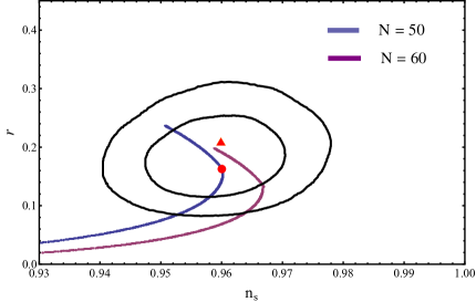
Figure 34: $r$ versus $n_{s}$ for the non-supersymmetric inflaton potential with $(j,~{}k,~{}l)=(2,~{}3,~{}4)$ where the inflationary trajectory is at the left of the maximum $\phi_{M2}$.

(4) When the slow-roll inflation occurs at the right of the maximum $\phi_{M2}$, i.e., $\phi_{M2}<\phi_{i}<\phi_{f}$, we will not study it here since it is the same as the above case (1).

Second, we study the supersymmetric models with inflaton potential $V=|a\phi+b\phi^{2}|^{2}=a^{2}\phi^{2}+2ab\phi^{3}+b^{2}\phi^{4}$. For simplicity, we assume $a>0$ while $b<0$. Thus, there exist a maximum at $\phi_{M}=-\frac{a}{2b}$ and two minima at $\phi_{m1}=0$ and $\phi_{m2}=-\frac{a}{b}$. And we shall consider the following four cases:

(1) When the slow-roll inflation occurs at the left of the minimum $\phi_{m1}$, i.e., $\phi_{i}<\phi_{f}<\phi_{m1}$, we present the numerical results for $r$ versus $n_{s}$ in Fig. 35. With $n_{s}$ in the $1\sigma$ range $0.9603\pm 0.0073$, the range of $r$ is $[0.1369,~{}0.2490]$, which can be consistent with the BICEP2 experiment. Moreover, for the number of e-folding $N_{e}=50$, $n_{s}$ and $r$ are within $1\sigma$ and $2\sigma$ regions of the BICEP2 experiment for $a>-30b$ and $a>-15b$, respectively. For the number of e-folding $N_{e}=60$, $n_{s}$ and $r$ are within $1\sigma$ region of the BICEP2 experiment for $a>-8b$ and are generically in $2\sigma$ region. Let us give two best fit points for the BICEP2 data. The best fit point with $n_{s}=0.96$ and $r=0.16$ can be realized for $N_{e}=50$, and $a\thickapprox-2000b$, for example, $a=2000$ and $b=-1$, and the corresponding $\phi_{i},~{}\phi_{f}$, and $\phi_{m1}$ are respectively $-14.2462,~{}-1.41521$, and $0$. Another best fit point with $n_{s}=0.959$ and $r=0.20$ can be obtained for $N_{e}=60$, and $a\thickapprox-26b$, for instance, $a=26$ and $b=-1$, and the corresponding $\phi_{i},~{}\phi_{f}$, and $\phi_{m1}$ are $-17.7247,~{}-1.49091$, and $0$, respectively.

(2) When the slow-roll inflation occurs at the right of the minimum $\phi_{m1}$ and the left of the maximum $\phi_{M}$, i.e., $\phi_{m1}<\phi_{f}<\phi_{i}<\phi_{M}$, to have relatively large $r$, we find that $|b|$ cannot be equal to or larger than $a$. The numerical results for $r$ versus $n_{s}$ are also given in Fig. 35. For $n_{s}$ in the $1\sigma$ range $0.9603\pm 0.0073$, the range of $r$ is $[0.0254,~{}0.1584]$, which can be consistent with the BICEP2 experiment. In addition, for the number of e-folding $N_{e}=50$, $n_{s}$ and $r$ are within $1\sigma$ and $2\sigma$ regions of the BICEP2 experiment for $a>-85b$ and $a>-47b$, respectively. For the number of e-folding $N_{e}=60$, $n_{s}$ and $r$ are within $2\sigma$ region for $a>-85b$, while no viable parameter space for $1\sigma$ region. Especially, the best fit point with $n_{s}=0.96$ and $r=0.158$ for the BICEP2 data can be obtained for $N_{e}=50$, and $a>-10^{4}b$. For example, $a=1$ and $b=-10^{-4}$, and the corresponding $\phi_{i},~{}\phi_{e}$, and $\phi_{M}$ respectively are $14.2025,~{}1.41391$, and $3333.33$.

Figure 35: $r$ versus $n_{s}$ for the supersymmetric inflaton potential with $(j,~{}k,~{}l)=(2,~{}3,~{}4)$ where the inflationary trajectories are at the left and right of the minimum $\phi_{m1}$.

(3) When the slow-roll inflation occurs at the right of the maximum $\phi_{M}$, i.e., $\phi_{M}<\phi_{i}<\phi_{f}<\phi_{m2}$, it is the same as the above case (2) and then we will not discuss it here.

(4) When the slow-roll inflation occurs at the right of the minimum $\phi_{m2}$, i.e., $\phi_{m2}<\phi_{f}<\phi_{i}$, we will not study it here since it is the same as the above case (1).

IV.11 The Most General Renormalizable Supersymemtric Inflationary Models

We briefly comment on the most general renormalizable supersymmetric inflationary models with the following inflaton potential

$$V = (a^{\prime}+b^{\prime}\phi^{\prime}+c^{\prime}\phi^{\prime 2})^{2}~{},~{}\,$$ (36)

where $a^{\prime}$, $b^{\prime}$, and $c^{\prime}$ are all non-zero. Redefining the inflaton field and parameters as follows

$$\phi~{}\equiv~{}\phi^{\prime}+\frac{b^{\prime}}{2c^{\prime}}~{},~{}~{}a~{}\equiv~{}a^{\prime}-\frac{b^{\prime 2}}{4c^{\prime}}~{},~{}b~{}\equiv~{}c^{\prime}~{}.~{}\,$$ (37)

we obtain the inflaton potential

$$V = (a+b\phi^{2})^{2}~{}.~{}\,$$ (38)

This is the same as the supersymmetric inflaton potential, which is studied in the subsection E. Thus, we will not repeat it here.

IV.12 Numerical Result Summary

To summarize the above results for $n_{s}$ within its $1\sigma$ range $0.9603\pm 0.0073$, we present the ranges of $r$ for different signs of parameters in the non-supersymmetric and supersymmetric models respectively in Tables 1 and 2. Interestingly, we always have large enough tensor-to-scalar ratios, which are within the reach of the future Planck and QUBIT experiments.

Table 1: The ranges of $r$ for different signs of parameters and $n_{s}$ within its $1\sigma$ range $0.9603\pm 0.0073$ in the non-supersymmetric models.

Model	Sign of the Parameters	Range I	Range II	Range III	Range IV
(0, 1, 2)	(+, +, $-$)	[0.0132, 0.0534]	[0.0132, 0.0534]
	(+, $-$, +)	[0.0132, 0.1610]	[0.0132, 0.1610]
(0, 1, 3)	(+, +, $-$)	[0.1231, 0.2237]	[0.0337, 0.0669]	[0.0085, 0.0482]
	(+, $-$, $-$)	[0.1670, 0.2427]
(0, 1, 4)	(+, +, $-$)	[0.0250, 0.0732]	[0.0077, 0.0459]
	(+, $-$, +)	NO FIT	[0.1288, 0.2498]
(0, 2, 3)	(+, +, $-$)	[0.1363, 0.2206]	[0.0645, 0.160]	[0.0097, 0.0431]
	(+, $-$, $-$)	[0.1249, 0.2242]	[0.0104, 0.0512]	[0.0099, 0.0505]
	(+, $-$, +)	[0.0099, 0.0485]	[0.0099, 0.0515]	[0.1232, 0.2253]
(0, 2, 4)	(+, +, $-$)	[0.0480, 0.1565]	[0.0072, 0.0444]
(0, 3, 4)	(+, +, $-$)	[0.0742, 0.1956]	[0.0067, 0.0454]
	(+, $-$, +)	[0.1995, 0.2473]	[0.1311, 0.2512]
(1, 2, 3)	(+, +, $-$)	[0.1234,0.2207]	[0.0337, 0.158]	[0.0083, 0.0471]
(1, 2, 4)	(+, +, $-$)	[0.0084, 0.0449]	[0.0487, 0.1585]	[0.0487, 0.1585]	[0.0084, 0.0449]
(1, 3, 4)	(+, +, $-$)	[0.0556, 0.2328]	[0.0081, 0.0458]
(2, 3, 4)	(+, +, $-$)	[0.0073, 0.0472]	[0.0496, 0.1585]	[0.0490, 0.2228]	[0.0073, 0.0472]

Table 2: The ranges of $r$ for different signs of parameters and $n_{s}$ within its $1\sigma$ range $0.9603\pm 0.0073$ in the supersymmetric models.

Model	Sign of the Parameters	Range I	Range II	Range III	Range IV
$|a+b\phi|^{2}$	(+, $-$)	[0.1322, 0.1584]	[0.1322, 0.1584]
$|a+b\phi^{2}|^{2}$	(+, $-$)	[0.1319, 0.2484]	[0.0254, 0.1585]	[0.0254, 0.1585]	[0.1319, 0.2484]
$|a\phi+b\phi^{2}|^{2}$	(+, $-$)	[0.1369, 0.2490]	[0.0254, 0.1369]	[0.0254, 0.1369]	[0.1369, 0.2490]

V Conclusion

We have systematically studied the renormalizable three-term polynomial inflation in the supersymmetric and non-supersymmetric models. We can construct the supersymmetric inflaton potentials via the supergravity theory, and we showed that the general renormalizable supergravity model is equivalent to one kind of our supersymmetric models. Although the running of the spectral index is out of the $2\sigma$ range for all the models, we found that the spectral index and tensor-to-scalar ratio can be consistent with the Planck and BICEP2 results. Even if we do not consider the BICEP2 experiment, our inflationary models can not only highly agree with the Planck observations, but also saturate its upper bound on the tensor-to-scalar ratio ($r\leq 0.11$). In short, our models can be tested at the future Planck and QUBIC experiments.

- (1) A. A. Starobinsky, Phys. Lett. B 91, 99 (1980).
- (2) A. H. Guth, Phys. Rev. D 23, 347 (1981).
- (3) A. D. Linde, Phys. Lett. B 108, 389 (1982).
- (4) A. Albrecht and P. J. Steinhardt, Phys. Rev. Lett. 48, 1220 (1982).
- (5) P. A. R. Ade et al. [Planck Collaboration], arXiv:1303.5062 [astro-ph.CO].
- (6) G. Hinshaw et al. [WMAP Collaboration], Astrophys. J. Suppl. 208, 19 (2013) [arXiv:1212.5226 [astro-ph.CO]].
- (7) S. Das, T. Louis, M. R. Nolta, G. E. Addison, E. S. Battistelli, J. R. Bond, E. Calabrese and D. C. M. J. Devlin et al., JCAP 1404, 014 (2014) [arXiv:1301.1037 [astro-ph.CO]].
- (8) R. Keisler, C. L. Reichardt, K. A. Aird, B. A. Benson, L. E. Bleem, J. E. Carlstrom, C. L. Chang and H. M. Cho et al., Astrophys. J. 743, 28 (2011) [arXiv:1105.3182 [astro-ph.CO]].
- (9) P. A. R. Ade et al. [Planck Collaboration], arXiv:1303.5076 [astro-ph.CO].
- (10) P. A. R. Ade et al. [Planck Collaboration], arXiv:1303.5082 [astro-ph.CO].
- (11) P. A. R. Ade et al. [BICEP2 Collaboration], arXiv:1403.3985 [astro-ph.CO].
- (12) P. A. R. Ade et al. [BICEP2 and Planck Collaborations], Phys. Rev. Lett. 114, no. 10, 101301 (2015) [arXiv:1502.00612 [astro-ph.CO]].
- (13) P. A. R. Ade et al. [Planck Collaboration], arXiv:1502.01589 [astro-ph.CO].
- (14) P. A. R. Ade et al. [Planck Collaboration], arXiv:1502.02114 [astro-ph.CO].
- (15) C. P. Burgess, M. Cicoli and F. Quevedo, JCAP 1311, 003 (2013) [arXiv:1306.3512, arXiv:1306.3512 [hep-th]].
- (16) D. H. Lyth, Phys. Rev. Lett. 78, 1861 (1997) [hep-ph/9606387].
- (17) L. A. Anchordoqui, V. Barger, H. Goldberg, X. Huang and D. Marfatia, arXiv:1403.4578 [hep-ph].
- (18) M. Czerny, T. Kobayashi and F. Takahashi, arXiv:1403.4589 [astro-ph.CO].
- (19) Y. Hamada, H. Kawai, K. -y. Oda and S. C. Park, arXiv:1403.5043 [hep-ph].
- (20) T. Kobayashi and O. Seto, Phys. Rev. D 89, 103524 (2014) [arXiv:1403.5055 [astro-ph.CO]].
- (21) S. Ferrara, A. Kehagias and A. Riotto, arXiv:1403.5531 [hep-th].
- (22) S. Choudhury and A. Mazumdar, arXiv:1403.5549 [hep-th].
- (23) Y. Gong, arXiv:1403.5716 [gr-qc].
- (24) A. Ashoorioon, K. Dimopoulos, M. M. Sheikh-Jabbari and G. Shiu, arXiv:1403.6099 [hep-th].
- (25) N. Okada, V. N. Şenoğuz and Q. Shafi, arXiv:1403.6403 [hep-ph].
- (26) J. Ellis, M. A. G. Garcia, D. V. Nanopoulos and K. A. Olive, arXiv:1403.7518 [hep-ph].
- (27) K. Hamaguchi, T. Moroi and T. Terada, Physics Letters B 733C (2014), pp. 305-308 [arXiv:1403.7521 [hep-ph]].
- (28) P. Di Bari, S. F. King, C. Luhn, A. Merle and A. Schmidt-May, arXiv:1404.0009 [hep-ph].
- (29) S. Kawai and N. Okada, arXiv:1404.1450 [hep-ph].
- (30) S. Antusch and D. Nolde, arXiv:1404.1821 [hep-ph].
- (31) B. Freivogel, M. Kleban, M. R. Martinez and L. Susskind, arXiv:1404.2274 [astro-ph.CO].
- (32) R. Bousso, D. Harlow and L. Senatore, arXiv:1404.2278 [astro-ph.CO].
- (33) N. Kaloper and A. Lawrence, arXiv:1404.2912 [hep-th].
- (34) S. Choudhury and A. Mazumdar, arXiv:1404.3398 [hep-th].
- (35) K. -Y. Choi and B. Kyae, arXiv:1404.3756 [hep-ph].
- (36) H. Murayama, K. Nakayama, F. Takahashi and T. T. Yanagida, arXiv:1404.3857 [hep-ph].
- (37) J. McDonald, arXiv:1404.4620 [hep-ph].
- (38) X. Gao, T. Li and P. Shukla, arXiv:1404.5230 [hep-ph].
- (39) Q. Gao, Y. Gong, T. Li and Y. Tian, Sci. China Phys. Mech. Astron. 57, 1442 (2014) [arXiv:1404.7214 [hep-th]].
- (40) T. Li, Z. Li and D. V. Nanopoulos, arXiv:1405.0197 [hep-th].
- (41) D. Chialva and A. Mazumdar, arXiv:1405.0513 [hep-th].
- (42) T. Li, Z. Li and D. V. Nanopoulos, JHEP 1407, 052 (2014) [arXiv:1405.1804 [hep-th]].
- (43) R. Kallosh, A. Linde and A. Westphal, arXiv:1405.0270 [hep-th].
- (44) Q. Gao, Y. Gong and T. Li, arXiv:1405.6451 [gr-qc].
- (45) X. Gao, T. Li and P. Shukla, arXiv:1406.0341 [hep-th].
- (46) K. Nakayama, F. Takahashi and T. T. Yanagida, arXiv:1406.4265 [hep-ph].
- (47) S. Choudhury and A. Mazumdar, Nucl. Phys. B 882, 386 (2014) [arXiv:1306.4496 [hep-ph]].
- (48) T. Li, Z. Li and D. V. Nanopoulos, arXiv:1407.1819 [hep-th].
- (49) I. Ben-Dayan, F. G. Pedro and A. Westphal, arXiv:1407.2562 [hep-th].
- (50) N. Okada and S. Okada, arXiv:1407.3544 [hep-ph].
- (51) D. Z. Freedman, P. van Nieuwenhuizen and S. Ferrara, Phys. Rev. D 13 (1976) 3214; S. Deser and B. Zumino, Phys. Lett. B 62 (1976) 335.
- (52) E. J. Copeland, A. R. Liddle, D. H. Lyth, E. D. Stewart and D. Wands, Phys. Rev. D 49, 6410 (1994) [astro-ph/9401011]; E. D. Stewart, Phys. Rev. D 51, 6847 (1995) [hep-ph/9405389]; Also see, for example: A. D. Linde, Particle Physics and Inflationary Cosmology (Harwood, Chur, Switzerland, 1990); D. H. Lyth and A. Riotto, Phys. Rep. 314 (1999) 1 [arXiv:hep-ph/9807278]. J. Martin, C. Ringeval and V. Vennin, arXiv:1303.3787 [astro-ph.CO]; M. Yamaguchi, Class. Quant. Grav. 28, 103001 (2011) [arXiv:1101.2488 [astro-ph.CO]].
- (53) A. S. Goncharov, A. D. Linde and M. I. Vysotsky, Phys. Lett. B 147, 279 (1984).
- (54) E. Cremmer, S. Ferrara, C. Kounnas and D. V. Nanopoulos, Phys. Lett. B 133, 61 (1983); J. R. Ellis, A. B. Lahanas, D. V. Nanopoulos and K. Tamvakis, Phys. Lett. B 134, 429 (1984); J. R. Ellis, C. Kounnas and D. V. Nanopoulos, Nucl. Phys. B 241, 406 (1984); Nucl. Phys. B 247, 373 (1984); A. B. Lahanas and D. V. Nanopoulos, Phys. Rept. 145, 1 (1987).
- (55) J. R. Ellis, K. Enqvist, D. V. Nanopoulos, K. A. Olive and M. Srednicki, Phys. Lett. B 152, 175 (1985) [Erratum-ibid. 156B, 452 (1985)].
- (56) K. Enqvist, D. V. Nanopoulos and M. Quiros, Phys. Lett. B 159, 249 (1985).
- (57) J. Ellis, D. V. Nanopoulos and K. A. Olive, Phys. Rev. Lett. 111, 111301 (2013) [arXiv:1305.1247 [hep-th]].
- (58) J. Ellis, D. V. Nanopoulos and K. A. Olive, JCAP 1310, 009 (2013) [arXiv:1307.3537 [hep-th]].
- (59) T. Li, Z. Li and D. V. Nanopoulos, arXiv:1310.3331 [hep-ph].
- (60) J. Ellis, D. V. Nanopoulos and K. A. Olive, arXiv:1310.4770 [hep-ph].
- (61) M. Kawasaki, M. Yamaguchi and T. Yanagida, Phys. Rev. Lett. 85, 3572 (2000) [hep-ph/0004243].
- (62) M. Yamaguchi and J. ’i. Yokoyama, Phys. Rev. D 63, 043506 (2001) [hep-ph/0007021].
- (63) M. Yamaguchi, Phys. Rev. D 64, 063502 (2001) [hep-ph/0103045].
- (64) M. Kawasaki and M. Yamaguchi, Phys. Rev. D 65, 103518 (2002) [hep-ph/0112093].
- (65) R. Kallosh and A. Linde, JCAP 1011, 011 (2010) [arXiv:1008.3375 [hep-th]].
- (66) R. Kallosh, A. Linde and T. Rube, Phys. Rev. D 83, 043507 (2011) [arXiv:1011.5945 [hep-th]].
- (67) K. Nakayama, F. Takahashi and T. T. Yanagida, Phys. Lett. B 725, 111 (2013) [arXiv:1303.7315 [hep-ph]].
- (68) K. Nakayama, F. Takahashi and T. T. Yanagida, JCAP 1308, 038 (2013) [arXiv:1305.5099 [hep-ph]].
- (69) F. Takahashi, Physics Letters B 727, 21 (2013) [arXiv:1308.4212 [hep-ph]].
- (70) T. Li, Z. Li and D. V. Nanopoulos, JCAP 1402, 028 (2014) [arXiv:1311.6770 [hep-ph]].
- (71) E. Battistelli et al. [QUBIC Collaboration], Astropart. Phys. 34, 705 (2011) [arXiv:1010.0645 [astro-ph.IM]].
- (72) D. H. Lyth and A. Riotto, Phys. Rept. 314, 1 (1999) [hep-ph/9807278].
- (73) E. D. Stewart and D. H. Lyth, Phys. Lett. B 302, 171 (1993) [gr-qc/9302019].
- (74) M. Kawasaki, M. Yamaguchi and T. Yanagida, Phys. Rev. D 63, 103514 (2001) [hep-ph/0011104].
- (75) A. Mazumdar, T. Noumi and M. Yamaguchi, Phys. Rev. D 90, no. 4, 043519 (2014) [arXiv:1405.3959 [hep-th]].
- (76) R. Allahverdi, K. Enqvist, J. Garcia-Bellido and A. Mazumdar, Phys. Rev. Lett. 97, 191304 (2006) [hep-ph/0605035].
- (77) R. Allahverdi, K. Enqvist, J. Garcia-Bellido, A. Jokinen and A. Mazumdar, JCAP 0706, 019 (2007) [hep-ph/0610134].
- (78) R. Allahverdi, B. Dutta and A. Mazumdar, Phys. Rev. D 78, 063507 (2008) [arXiv:0806.4557 [hep-ph]].
- (79) K. Enqvist, A. Mazumdar and P. Stephens, JCAP 1006, 020 (2010) [arXiv:1004.3724 [hep-ph]].