Hypothesis setting and order statistic for
robust genomic meta-analysis

Abstract

Meta-analysis techniques have been widely developed and applied in genomic applications, especially for combining multiple transcriptomic studies. In this paper we propose an order statistic of $p$-values ($r$th ordered $p$-value, rOP) across combined studies as the test statistic. We illustrate different hypothesis settings that detect gene markers differentially expressed (DE) “in all studies,” “in the majority of studies” or “in one or more studies,” and specify rOP as a suitable method for detecting DE genes “in the majority of studies.” We develop methods to estimate the parameter $r$ in rOP for real applications. Statistical properties such as its asymptotic behavior and a one-sided testing correction for detecting markers of concordant expression changes are explored. Power calculation and simulation show better performance of rOP compared to classical Fisher’s method, Stouffer’s method, minimum $p$-value method and maximum $p$-value method under the focused hypothesis setting. Theoretically, rOP is found connected to the naïve vote counting method and can be viewed as a generalized form of vote counting with better statistical properties. The method is applied to three microarray meta-analysis examples including major depressive disorder, brain cancer and diabetes. The results demonstrate rOP as a more generalizable, robust and sensitive statistical framework to detect disease-related markers.

and T1Supported by NIH R21MH094862 and R01DA016750.

1 Introduction

With the advances in high-throughput experimental technology in the past decade, the production of genomic data has become affordable and thus prevalent in biomedical research. Accumulation of experimental data in the public domain has grown rapidly, particularly of microarray data for gene expression analysis and single nucleotide polymorphism (SNP) genotyping data for genome-wide association studies (GWAS). For example, the Gene Expression Omnibus (GEO; http://www.ncbi.nlm.nih.gov/geo/) from the National Center for Biotechnology Information (NCBI) and the Gene Expression Atlas (http://www.ebi.ac.uk/gxa/) from the European Bioinformatics Institute (EBI) are the two largest public depository websites for gene expression data and the database of Genotypes and Phenotypes (dbGaP, http://www.ncbi.nlm.nih.gov/gap/) has the largest collection of genotype data. Because individual studies usually contain limited numbers of samples and the reproducibility of genomic studies is relatively low, the generalizability of their conclusions is often criticized. Therefore, combining multiple studies to improve statistical power and to provide validated conclusions has emerged as a common practice [see recent review papers by Tseng, Ghosh and Feingold (2012) and Begum et al. (2012)]. Such genomic meta-analysis is particularly useful in microarray analysis and GWAS. In this paper we focus on microarray meta-analysis while the proposed methodology can be applied to the traditional “univariate” meta-analysis or other types of genomic meta-analysis.

Microarray experiments measure transcriptional activities of thousands of genes simultaneously. One commonly seen application of microarray data is to detect differentially expressed (DE) genes in samples labeled with two conditions (e.g., tumor recurrence versus nonrecurrence), multiple conditions (e.g., multiple tumor subtypes), survival information or time series. In the literature, microarray meta-analysis usually refers to combining multiple studies of related hypotheses or conditions to better detect DE genes (also called candidate biomarkers). For this problem, two major types of statistical procedures have been used: combining effect sizes or combining $p$-values. Generally speaking, no single method performs uniformly better than the others in all data sets for various biological objectives, both from a theoretical point of view [Littell and Folks (1971, 1973)] and from empirical experiences. In combining effect sizes, the fixed effects model and the random effects model are the most popular methods [Cooper, Hedges and Valentine (2009)]. These methods are usually more straightforward and powerful to directly synthesize information of the effect size estimates, compared to $p$-value combination methods. They are, however, only applicable to samples with two conditions when the effect sizes can be defined and combined. On the other hand, methods combining $p$-values provide better flexibility for various outcome conditions as long as $p$-values can be assessed for integration. Fisher’s method is among the earliest $p$-value methods applied to microarray meta-analysis [Rhodes et al. (2002)]. It sums the log-transformed $p$-values to aggregate statistical significance across studies. Under the null hypothesis, assuming that the studies are independent and the hypothesis testing procedure correctly fits the observed data, Fisher’s statistic follows a chi-squared distribution with degrees of freedom $2K$, where $K$ is the number of studies combined. Other methods such as Stouffer’s method [Stouffer et al. (1949)], the minP method [Tippett (1931)] and the maxP method [Wilkinson (1951)] have also been widely used in microarray meta-analysis. It can be shown that these test statistics have simple analytical forms of null distributions and, thus, they are easy to apply to the genomic settings. The assumptions and hypothesis settings behind these methods are, however, very different and have not been carefully considered in most microarray meta-analysis applications so far. In Fisher, Stouffer and minP, the methods detect markers that are differentially expressed in “one or more” studies (see the definition of $\mathrm{HS}_{B}$ in Section 2.1). In other words, an extremely small $p$-value in one study is usually enough to impact the meta-analysis and cause statistical significance. On the contrary, methods like maxP tend to detect markers that are differentially expressed in “all” studies (called $\mathrm{HS}_{A}$ in Section 2.1) since maxP requires that all combined $p$-values are small for a marker to be detected. In this paper, we begin in Section 2.1 to elucidate the hypothesis settings and biological implications behind these methods. In many meta-analysis applications, detecting markers differentially expressed in all studies is more appealing. The requirement of DE in “all” studies, however, is too stringent when $K$ is large and in light of the fact that experimental data are peppered with noisy measurements from probe design, sample collection, data generation and analysis. Thus, we describe in Section 2.1 a robust hypothesis setting (called $\mathrm{HS}_{r}$) that detects biomarkers differentially expressed “in the majority of” studies (e.g., $>$70% of the studies) and we propose a robust order statistic, the $r$th ordered $p$-value (rOP), for this hypothesis setting.

The remainder of this paper is structured as follows to develop the rOP method. In Section 2.2 the rationale and algorithm of rOP are outlined, and the methods for parameter estimation are described in Section 2.3. Section 2.4 extends rOP with a one-sided test correction to avoid detection of DE genes with discordant fold change directions across studies. Section 3 demonstrates applications of rOP to three examples in brain cancer, major depressive disorder (MDD) and diabetes, and compares the result with other classical meta-analysis methods. We further explore power calculation and asymptotic properties of rOP in Section 4.1, and evaluate rOP in genomic settings by simulation in Section 4.2. We also establish an unexpected but insightful connection of rOP with the classical naïve vote counting method in Section 4.3. Section 5 contains final conclusions and discussions.

2 $r$th ordered $p$-value (rOP)

2.1 Hypothesis settings and motivation

We consider the situation when $K$ transcriptomic studies are combined for a meta-analysis where each study contains $G$ genes for information integration. Denote by $\theta_{gk}$ the underlying true effect size for gene $g$ and study $k$ ($1\leq g\leq G$, $1\leq k\leq K$). For a given gene $g$, we follow the convention of Birnbaum (1954) and Li and Tseng (2011) to consider two complementary hypothesis settings, depending on the pursuit of different types of targeted markers:

$$\mathrm{HS}_{A}\dvtx\biggl{\{}H_{0}\dvtx\bigcap_{k}\{\theta_{gk}=0\}\mbox{ versus }H_{a}^{(A)}\dvtx\bigcap_{k}\{\theta_{gk}\neq 0\}\biggr{\}},$$

$$\mathrm{HS}_{B}\dvtx\biggl{\{}H_{0}\dvtx\bigcap_{k}\{\theta_{gk}=0\}\mbox{ versus }H_{a}^{(B)}\dvtx\bigcup_{k}\{\theta_{gk}\neq 0\}\biggr{\}}.$$

In $\mathrm{HS}_{A}$, the targeted biomarkers are those differentially expressed in all studies (i.e., the alternative hypothesis is the intersection event that effect sizes of all $K$ studies are nonzero), while $\mathrm{HS}_{B}$ pursues biomarkers differentially expressed in one or more studies (the alternative hypothesis is the union event instead of the intersection in $\mathrm{HS}_{A}$). Biologically speaking, $\mathrm{HS}_{A}$ is more stringent and more desirable to identify consistent biomarkers across all studies if the studies are homogeneous. $\mathrm{HS}_{B}$, however, is useful when heterogeneity is expected. For example, if studies analyzing different tissues are combined (e.g., study 1 uses epithelial tissues and study 2 uses blood samples), it is reasonable to identify tissue-specific biomarkers detected by $\mathrm{HS}_{B}$. We note that $\mathrm{HS}_{B}$ is identical to the classical union-intersection test (UIT) [Roy (1953)] but $\mathrm{HS}_{A}$ is different from the intersection-union test (IUT) [Berger (1982), Berger and Hsu (1996)]. In IUT, the statistical hypothesis is in a complementary form between the null and alternative hypotheses $\{H_{0}\dvtx\bigcup_{k}\{\theta_{gk}=0\}$ versus $H_{a}^{(A)}\dvtx\bigcap_{k}\{\theta_{gk}\neq 0\}\}$. Solutions for IUT require a more sophisticated mixture or Bayesian modeling to accommodate the composite null hypothesis and are not the focus of this paper [for more details, see Erickson, Kim and Allison (2009)].

As discussed in Tseng, Ghosh and Feingold (2012), most existing genomic meta-analysis methods target on $\mathrm{HS}_{B}$. Popular methods include classical Fisher’s method [sum of minus log-transformed $p$-values; Fisher (1925)], Stouffer’s method [sum of inverse-normal-transformed $p$-values; Stouffer et al. (1949)], minP [minimum of combined $p$-values; Tippett (1931)] and a recently proposed adaptively weighted (AW) Fisher’s method [Li and Tseng (2011)]. The random effects model targets on a slight variation of $\mathrm{HS}_{A}$, where the effect sizes in the alternative hypothesis are random effects drawn from a Gaussian distribution centered away from zero (but are not guaranteed to be all nonzero). The maximum $p$-value method (maxP) is probably the only method available to specifically target on $\mathrm{HS}_{A}$ so far. By taking the maximum of $p$-values from combined studies as the test statistic, the method requires that all $p$-values be small for a gene to be detected. Assuming independence across studies and that the inferences to generate $p$-values in single studies are correctly specified, $p$-values ($p_{k}$ as the $p$-value of study $k$) are i.i.d. uniformly distributed in $[0,1]$. Fisher’s statistic ($S^{\mathrm{Fisher}}=-2\sum\log p_{k}$) follows a chi-squared distribution with degree of freedom $2K$ [i.e., $S^{\mathrm{Fisher}}\sim\chi^{2}(2K)$] under null hypothesis $H_{0}$; Stouffer’s statistic [$S^{\mathrm{Stouffer}}=\sum\Phi^{-1}(1-p_{k})$, where $\Phi^{-1}(\cdot)$ is the quantile function of a standard normal distribution] follows a normal distribution with variance $K$ [i.e., $S^{\mathrm{Stouffer}}\sim N(0,K)$]; minP statistic ($S^{\mathrm{minP}}=\min\{p_{k}\}$) follows a Beta distribution with parameters 1 and $K$ [i.e., $S^{\mathrm{minP}}\sim\operatorname{Beta}(1,K)$]; and maxP statistic ($S^{\mathrm{maxP}}=\max\{p_{k}\}$) follows a Beta distribution with parameters $K$ and 1 [i.e., $S^{\mathrm{maxP}}\sim\operatorname{Beta}(K,1)$].

The $\mathrm{HS}_{A}$ hypothesis setting and maxP method are obviously too stringent in light of the generally noisy nature of microarray experiments. When $K$ is large, $\mathrm{HS}_{A}$ is not robust and inevitably detects very few genes. Instead of requiring differential expression in all studies, biologists are more interested in, for example, “biomarkers that are differentially expressed in more than 70% of the combined studies.” Denote by $\Theta_{h}=\{\sum_{k=1}^{K}I(\theta_{gk}\neq 0)=h\}$ the situation that exactly $h$ out of $K$ studies are differentially expressed. The new robust hypothesis setting becomes

$$\mathrm{HS}_{r}\dvtx\Biggl{\{}H_{0}\dvtx\bigcap_{k}\{\theta_{gk}=0\}\mbox{ versus }H_{a}^{(r)}\dvtx\bigcup_{h=r}^{K}\Theta_{h}\Biggr{\}},$$

where $r=\lceil p\cdot K\rceil$, $\lceil x\rceil$ is the smallest integer no less than $x$ and $p$ ($0<p\leq 1$) is the minimal percentage of studies required to call differential expression (e.g., $p=70\%$). We note that $\mathrm{HS}_{A}$ and $\mathrm{HS}_{B}$ are both special cases of the extended $\mathrm{HS}_{r}$ class (i.e., $\mathrm{HS}_{A}=\mathrm{HS}_{K}$ and $\mathrm{HS}_{B}=\mathrm{HS}_{1}$), but we will focus on large $r$ (i.e., $p>50\%$) in this paper and view $\mathrm{HS}_{r}$ as a relaxed and robust form of $\mathrm{HS}_{A}$.

=250pt Gene A Gene B Gene C Gene D Study 1 $0.1$ 1e–20[*]tt $0.25$ $0.15$ Study 2 $0.1$ $0.9$ $0.25$ $0.15$ Study 3 $0.1$ $0.9$ $0.25$ $0.15$ Study 4 $0.1$ $0.9$ $0.25$ $0.15$ Study 5 $0.1$ $0.9$ $0.25$ $0.9$ Fisher ($\mathrm{HS}_{B}$) $0.01\tabnoteref[*]{tt}$ 1e–15[*]tt $0.18$ $0.12$ Stouffer ($\mathrm{HS}_{B}$) $0.002\tabnoteref[*]{tt}$ $0.03\tabnoteref[*]{tt}$ $0.07$ $0.10$ minP ($\mathrm{HS}_{B}$) $0.41$ 5e–20[*]tt $0.76$ $0.56$ maxP ($\mathrm{HS}_{A}$) 1e–5[*]tt $0.59$ $0.001\tabnoteref[*]{tt}$ $0.59$ rOP ($r=4$) ($\mathrm{HS}_{r}$) 5e–4[*]tt $0.92$ $0.015\tabnoteref[*]{tt}$ $0.002\tabnoteref[*]{tt}$ [*]tt$p$-values smaller than 0.05.

Table 1: Four hypothetical genes to compare different meta-analysis methods and to illustrate the motivation of rOP

In the literature, maxP has been used for $\mathrm{HS}_{A}$ and minP has been used for $\mathrm{HS}_{B}$. An intuitive extension of these two methods for $\mathrm{HS}_{r}$ is to use the $r$th ordered $p$-value (rOP). Before introducing the algorithm and properties of rOP, we illustrate the motivation of it by the following example. Suppose we consider four genes in five studies: gene A has marginally significant $p$-values ($p=0.1$) in all five studies; gene B has a strong $p$-value in study 1 ($p={}$1e–20) but $p=0.9$ in the other four studies; gene C is similar to gene A but has much weaker statistical significance ($p=0.25$ in all five studies); gene D differs from gene C in that studies 1–4 have small $p$-values ($p=0.15$) but study 5 has a large $p$-value ($p=0.9$). Table 1 shows the resulting $p$-values from five meta-analysis methods that are derived from classical parametric inference in Section 1. Comparing Fisher and minP in $\mathrm{HS}_{B}$, minP is sensitive to a study that has a very small $p$-value (see gene B) while Fisher, as an evidence aggregation method, is more sensitive when all or most studies are marginally statistically significant (e.g., gene A). Stouffer behaves similarly to Fisher except that it is less sensitive to the extremely small $p$-value in gene B. When we turn our attention to $\mathrm{HS}_{A}$, gene C and gene D cannot be detected by all three of the Fisher, Stouffer and minP methods. Gene C can be detected by both maxP and rOP as expected ($p=0.001$ and $0.015$, resp.). For gene D, it cannot be identified by the maxP method ($p=0.59$) but can be detected by rOP at $r=4$ ($p=0.002$). Gene D gives a good motivating example that maxP may be too stringent when many studies are combined and rOP provides additional robustness when one or a small portion of studies are not statistically significant. In genomic meta-analysis, genes similar to gene D are common due to the noisy nature of high-throughput genomic experiments or when a low-quality study is accidentally included in the meta-analysis. Although the types of desired markers (under $\mathrm{HS}_{A}$, $\mathrm{HS}_{B}$ or $\mathrm{HS}_{r}$) depend on the biological goal of a specific application, genes A, C and D are normally desirable marker candidates that researchers wish to detect in most situations while gene B is not (unless study-specific markers are expected as mentioned in Section 1). This toy example motivates the development of a robust order statistic of rOP below.

2.2 The rOP method

Below is the algorithm for rOP when the parameter $r$ is fixed. For a given gene $g$, without loss of generality, we ignore the subscript $g$ and denote by $S_{r}=p_{(r)}$, where $p_{(r)}$ is the $r$th order statistic of $p$-values $\{p_{1},p_{2},\ldots,p_{K}\}$. Under the null hypothesis $H_{0}$, $S_{r}$ follows a beta distribution with shape parameters $r$ and $K-r+1$, assuming that the model to generate $p$-values under the null hypothesis is correctly specified and all studies are independent. To implement rOP, one may apply this parametric null distribution to calculate the $p$-values for all genes and perform a Benjamini–Hochberg (BH) correction [Benjamini and Hochberg (1995)] to control the false discovery rate (FDR) under the general dependence structure. The Benjamini–Hochberg procedure can control the FDR at the nominal level or less when the multiple comparisons are independent or positively dependent. Although the Benjamini–Yekutieli (BY) procedure can be applied to a more general dependence structure of the comparisons, it is often too conservative and unnecessary [Benjamini and Yekutieli (2001)], especially in gene expression analysis where the comparisons are more likely to be positively dependent and the effect sizes are usually small to moderate (also see Section 4.2 for simulation results). As a result, we will not consider the BY procedure in this paper. The parametric BH approach has the advantage of fast computation, but in many situations the parametric beta null distribution may be violated because the assumptions to obtain $p$-values from each single study are not met and the null distributions of $p$-values are not uniformly distributed. When such violations of assumptions are suspected, we alternatively recommend a conventional permutation analysis (PA) instead. Class labels of the samples in each study are randomly permuted and the entire DE and meta-analysis procedures are followed. The permutation is repeated for $B$ times ($B=500$ in this paper) to simulate the null distribution and assess the $p$-values and $q$-values. The permutation analysis is used for all meta-analysis methods (including rOP, Fisher, Stouffer, minP and maxP) in this paper unless otherwise stated.

We note that both minP and maxP are special cases of rOP, but in this paper we mainly consider properties of rOP as a robust form of maxP (specifically, $K/2\leq r\leq K$).

2.3 Selection of $r$ in an application

The best selection of $r$ should depend on the biological interests. Ideally, $r$ is a tuning parameter that is selected by the biologists based on the biological questions asked and the experimental designs of the studies. However, in many cases, biologists may not have a strong prior knowledge for the selection of $r$ and data-driven methods for estimating $r$ may provide additional guidance in applications. The purpose of selecting $r<K$ is to tolerate potentially outlying studies and noises in the data. The noises may come from experimental limitations (e.g., failure in probe design, erroneous gene annotation or bias from experimental protocol) or heterogeneous patient cohorts in different studies. Another extreme case may come from inappropriate inclusion of a low-quality study into the genomic meta-analysis. Below we introduce two complementary guidelines to help select $r$ for rOP. The first method comes from the adjusted number of detected DE genes and the second is based on pathway association (a.k.a. gene set analysis), incorporating external biological knowledge.

2.3.1 Evaluation based on the number of detected DE genes

In the first method, we use a heuristic criterion to find the best $r$ such that the number of detected DE genes is the largest. The dashed line in Figure 1(a) shows the number of detected DE genes using different $r$ in rOP in a brain cancer application. The result shows a general decreasing trend in the number of detected DE genes when $r$ increases. However, when we randomly permute the $p$-values across genes within each study, the detected number of DE genes also shows a bias toward small $r$’s (dotted line). It shows that a large number of DE genes can be detected by a small $r$ (e.g., $r=1$ or 2) simply by chance. To eliminate this artifact, we apply a detrending method by subtracting the dotted permuted baseline from the dashed line. The resulting adjusted number of DE genes (solid line) is then used to seek the maximum that correspond to the suggested $r$. This detrend adjustment is similar to what was used in the GAP statistic [Tibshirani, Walther and Hastie (2001)] when estimating the number of clusters in cluster analysis. In such a scenario, the curve of number of clusters (on $x$-axis) versus sum of squared within-cluster dispersions is used to estimate the number of clusters. The curve always has a decreasing trend even in random data sets and the goal is usually to find an “elbow-like” turning point. The GAP statistic permutes the data to generate a baseline curve and subtract it from the observed curve. The problem becomes finding the maximum point in the detrended curve, a setting very similar to ours.

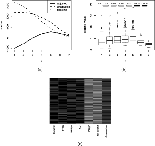
Figure 1: Results of brain cancer data set applying rOP. (a) Adjusted and unadjusted number of detected DE genes using different $r$. (b) Boxplots of $-\log(p)$ for the biological association evaluation. $p$-values for Wilcoxon signed-rank tests are shown on the top. Black filled rectangles represent a $p$-value smaller than 0.05. (c) Heatmap to show effective studies of rOP in each gene. Effective studies are shown in black and noneffective ones are in light gray.

Below we describe the algorithm for the first criterion. Using the original $K$ studies, the number of DE genes detected by rOP using different $r$ ($1\leq r\leq K$) is first calculated as $N_{r}$ [under the certain false discovery rate threshold, e.g., $\mathrm{FDR}=5\%$; see dashed line in Figure 1(a)]. We then randomly permute $p$-values in each study independently and recalculate the number of DE genes as $N_{r}^{(b)}$ in the $b$th permutation. The permutation is repeated for $B$ times ($B=100$ in this paper) and the adjusted number of detected DE genes is defined as $N^{\prime}_{r}=N_{r}-\sum_{b=1}^{B}N_{r}^{(b)}/B$ [see solid line in Figure 1(a)]. In other words, the adjusted number of DE genes is detrended so that it is purely contributed by the consistent DE information among studies. The parameter $r$ is selected so that $N^{\prime}_{r}$ is maximized (or we manually select $r$ as large as possible when $N^{\prime}_{r}$ reaches among the largest).

Remark 1.

Note that $N^{\prime}_{r}$ could sometimes be negative. This happens mostly when the signal in a single study is strong and $r$ is small. However, since we usually apply rOP for relatively large $K$ and $r$, the negative value is usually not an issue. We also note that, unlike the GAP statistic, the criterion to choose $r$ with the maximal adjusted number of detected DE genes is heuristic and has no theoretical guarantee. In simulations and real applications to be shown later, this method performs well and provides results consistent with the second criterion described below.

2.3.2 Evaluation based on biological association

Pathway analysis (a.k.a. gene set analysis) is a statistical tool to infer the correlation of differential expression evidence in the data with pathway knowledge (usually sets of genes with known common biological function or interactions) from established databases. In this approach, we hypothesize that the best selection of $r$ will produce a DE analysis result that generates the strongest statistical association with “important” (i.e., disease-related) pathways. Such pathways can be provided by biologists or obtained from pathway databases. However, it is well recognized that our understanding of biological and disease-related pathways are relatively poor and subject to change every few years. This is especially true for many complex diseases, such as cancers, psychiatric disorders and diabetes. In this case, it is more practical to use computational methods to generate “pseudo” disease-related pathways that are further reviewed by biologists before being utilized to estimate $r$. Below, we develop a computational procedure for selecting disease-related pathways. We perform pathway analysis using a large pathway database (e.g., GO, KEGG or BioCarta) and select pathways that are top ranked by aggregated committee decision of different $r$ from rOP. The detailed algorithm is as follows:

Step I.

Identification of disease-related pathways (committee decision by $[K/2]+1\leq r\leq K$):

1. [3.]

2. Apply rOP method to combine studies and generate $p$-values for each gene. Run through different $r$, $[K/2]+1\leq r\leq K$.

3. For a given pathway $m$, apply Kolmogorov–Smirnov test to compare the $p$-values of genes in the pathway and those outside the pathway. The pathway enrichment $p$-values are generated as $p_{r,m}$. Its rank among all pathways for a given $r$ is calculated as $R_{r,m}=\mathrm{rank}_{m}(p_{r,m})$. Small ranks suggest strong pathway enrichment for pathway $m$.

4. The sums of ranks of different $r$ are calculated as $S_{m}=\sum_{r=[K/2]+1}^{K}R_{r,m}$. The top $U=100$ pathways with the smallest $S_{m}$ scores are selected and denoted as $M$. We treat $M$ as the “pseudo” disease-related pathway set.

Step II.

Sequential testing of improved pathway enrichment significance:

1. [2.]

2. We perform sequential hypothesis testing that starts from $r^{\prime}=K$ since conceptually we would like to pick $r$ as large as possible. We first perform a Wilcoxon signed-rank test to test for difference of pathway enrichment significance for $r^{\prime}=K$ and $r^{\prime}=K-1$. In other words, we perform a two-sample test on the paired vectors of $(p_{K,m};m\in M)$ and $(p_{K-1,m};m\in M)$ and record the $p$-value as $\tilde{p}_{K,K-1}$.

3. If the test is rejected (using the conventional type I error of 0.05), it indicates that reducing from $r=K$ to $r=K-1$ can generate a DE gene list that produce more significant pathway enrichment in $M$. We will continue to reduce $r^{\prime}$ by one (i.e., $r^{\prime}=K-1$) and repeat the test between $(p_{r^{\prime},m};m\in M)$ and $(p_{r^{\prime}-1,m};m\in M)$. Similarly, the resulting $p$-values are recorded as $\tilde{p}_{r^{\prime},r^{\prime}-1}$. The procedure is repeated until the test from $r^{\prime}$ is not rejected. The final $r^{\prime}$ is selected for rOP.

Remark 2.

Note that for simplicity and since this evaluation should be examined together with the first criterion in Section 2.3.1, we will not perform $p$-value correction for multiple comparison or sequentially dependent hypothesis testings here. Practically, we suggest to select $r$ based on the diagnostic plots of the two criteria simultaneously. Examples of the selection will be shown in Section 3.

Remark 3.

We have tested different $U$ in real applications. As can be expected, the selection of $U$ did not affect the result much. In supplement Figure 7 [Song and Tseng (2014d)], we show that the ranks for rOP with different selection of $r$ as well as other methods become stable enough when $U=100$ for all our applications.

2.4 One-sided test modification to avoid discordant effect sizes

Methods combining effect sizes (e.g., random or fixed effects models) are suitable to combine studies with binary outcome, in which case the effect sizes are well defined as the standardized mean differences or odds ratios. Methods combining $p$-values, however, have advantages in combining studies with nonbinary outcomes (e.g., multi-class, continuous or censored data), in which case the F-test, simple linear regression or the Cox proportional hazard model can be used to generate $p$-values for integration. On the other hand, $p$-value combination methods usually combine two-sided $p$-values in binary outcome data. A gene may be found statistically significant with up-regulation in one study and down-regulation in another study. Such a confusing discordance, although sometimes a reflection of the biological truth, is often undesirable in most applications. Therefore, we make a one-sided test modification to the rOP method similar to the modification that Owen (2009) and Pearson (1934) applied on Fisher’s method. The modified rOP statistic is defined as the minimum of the two rOP statistics combining the one-sided tests of both tails. Details of this test statistic can be found in the supplementary material [Song and Tseng (2014a)].

3 Applications

We applied rOP as well as other meta-analysis methods to three microarray meta-analysis applications with different strengths of DE signal and different degrees of heterogeneity. Supplement Table 1A–C [Song and Tseng (2014c)] list the detailed information on seven brain cancer studies, nine major depressive disorder (MDD) studies and 16 diabetes studies for meta-analysis. Data were preprocessed and normalized by standard procedures in each array platform. Affymetrix data sets were processed by the RMA method and Illumina data sets were processed by manufacturer’s software with quantile normalization for probe analysis. Probes were matched to the same gene symbols. When multiple probes (or probe sets) matched to one gene symbol, the probe that contained the largest variability (i.e., inter-quartile range) was used to represent the gene. After gene matching and filtering, 5836, 7577 and 6645 genes remained in the brain cancer, MDD and diabetes data sets, respectively. The brain cancer studies were collected from the GEO database. The MDD studies were obtained from Dr. Etienne Sibille’s lab. A random intercept model adjusted for potential confounders was applied to each MDD study to obtain $p$-values [Wang et al. (2012a)]. Preprocessed data of 16 diabetes studies described by Park et al. (2009) were obtained from the authors. For studies with multiple groups, we followed the procedure of Park et al. by taking the minimum $p$-value of all the pairwise comparisons and adjusted for multiple tests. All the pathways used in this paper were downloaded from the Molecular Signatures Database [MSigDB, Subramanian et al. (2005)]. Pathway collections c2, c3 and c5 were used for the $r$ selection purpose.

3.1 Application of rOP

In all three applications, we demonstrate the estimation of $r$ for rOP using the two evaluation criteria in Section 2.3. In the first data set, two important subtypes of brain tumors—anaplastic astrocytoma (AA) and glioblastoma multiforme (GBM)—were compared in seven microarray studies. To estimate an adequate $r$ for the rOP application, we calculated the unadjusted number, the baseline number from permutation and the adjusted number of detected DE genes using $1\leq r\leq 7$ under FDR${}=5\%$ [Figure 1(a)]. The result showed a peak at $r=5$. For the second estimation method by pathway analysis, boxplots of $-\log_{10}(p)$ ($p$-values calculated from association of DE gene list with top pathways) versus $r$ were plotted [Figure 1(b)]. The Wilcoxon signed-rank tests showed that the result from $r=6$ is significantly more associated with pathways than that from $r=7$ ($p={}$2.7e–11) and similarly for $r=5$ versus $r=6$ ($p={}$4.4e–9). Combining the results from Figure 1(a) and (b), we decided to choose $r=5$ for this application. Figure 1(c) shows the heatmap of studies effective in rOP (when $r=5$) for each detected DE gene (a total of 1469 DE genes on the rows and seven studies on the columns). For example, if $p$-values for the seven studies are $(0.13,0.11,0.03,0.001,0.4,0.7,0.15)$, the test statistic for rOP is $S^{\mathrm{rOP}}=0.15$ and the five effective studies that contribute to rOP are indicated as $(1,1,1,1,0,0,1)$. In the heatmap, effective studies were indicated by black color and noneffective studies were in light gray. As shown in Figure 1(c), Paugh and Yamanaka were noneffective studies in almost all detected DE genes, suggesting that the two studies did not contribute to the meta-analysis and may potentially be problematic studies. This finding agrees with a recent MetaQC assessment result using the same seven studies [Kang et al. (2012)]. In our application, AA and GBM patients were compared in all seven studies. We expected to detect biomarkers that have consistent fold-change direction across studies and the one-sided corrected rOP method was more preferable. Supplement Figure 1 [Song and Tseng (2014d)] showed plots similar to Figure 1 for one-sided corrected rOP. The result similarly concluded that $r=5$ was the most suitable choice for this application.

For the second application, nine microarray studies used different areas of post-mortem brain tissues from MDD patients and control samples (supplement Table 1B [Song and Tseng (2014c)]). MDD is a complex genetic disease with largely unknown disease mechanism and gene regulatory networks. The postmortem brain tissues usually result in weak signals, compared to blood or tumor tissues, which makes meta-analysis an appealing approach. In supplement Figure 2(a) [Song and Tseng (2014d)], the maximizer of adjusted DE gene detection was at $r=6$ ($r=7$ or $8$ is also a good choice). For supplement Figure 2(b), the statistical significance improved “from $r=9$ to $r=8$” ($p={}$5.6e–14), “from $r=8$ to $r=7$” ($p={}$8.7e–7) and “from $r=7$ to $r=6$” ($p=0.045$). We also obtained 98 pathways that were potentially related to MDD from Dr. Etienne Sibille. As shown in supplement Figure 2(c), the statistical significance improved “from $r=8$ to $r=7$” using the 98 expert selected pathways. Combining the results, we decided to choose $r=7$ (since $r=6$ only provided marginal improvement in both criteria and we preferred $r$ as large as possible) for the rOP method in this application. Supplement Figure 2(d) showed the heatmap of effective studies in rOP. No obvious problematic study was observed. The one-sided rOP was also applied (results not shown); good selection of $r$ appeared to be between 5 and 7.

In the last application, 16 diabetes microarray studies were combined. These 16 studies were very heterogeneous in terms of the organisms, tissues and experimental design (supplement Table 1C [Song and Tseng (2014c)]). Supplement Figure 7 [Song and Tseng (2014d)] showed diagnostic plots to estimate $r$. Although the number of studies and heterogeneity across data sets were relatively larger than the previous two examples, we could still observe similar trends in supplement Figure 7. Specifically, for supplement Figure 3(a), it was shown that $r=7$–12 detected a higher adjusted number of DE genes. For pathway analysis, results from $r=12$ were more associated with the top pathways. As a result, we decided to use $r=12$ in this application. It was noticeable that the $r$ selection in this diabetes example was relatively vague compared to the previous examples. Supplement Figure 3(c) showed the heatmap of effective studies in rOP. Two to four studies (s01, s05, s08 and s14) appeared to be candidates of problematic studies, but the evidence was not as clear as the brain cancer example in Figure 1(c). It should be noted that the results of supplement Figure 3 used the beta null distribution inference and Benjamini–Hochberg correction. Permutation analysis generated a relatively unstable result (supplement Figure 4), although it suggested a similar selection of $r$. This was possibly due to the unusual ad hoc DE analysis from minimum $p$-values of all possible pairs of comparisons [procedures that were used in the original paper Park et al. (2009)].

Next, we explored the robustness of rOP by mixing a randomly chosen MDD study into seven brain cancer studies as an outlier. The results in supplement Figure 5 [Song and Tseng (2014d)] showed that $r=5$ or $6$ may be a good choice [supplement Figure 5(a) and (b)]. We used $r=6$ in rOP for this application. Supplement Figure 5(c) interestingly showed that the mixed MDD study, together with the Paugh and Yamanaka studies, was a potentially problematic study in the rOP meta-analysis. This result verified our intuition that rOP is robust to outlying studies and the $p$-values of the outlying studies minimally contribute to the rOP statistic.

3.2 Comparison of rOP with other meta-analysis methods

We performed rOP using $r$ determined from Section 3.1 in four applications (brain cancer, MDD, diabetes and brain cancer $+$ 1 random MDD) and compared to Fisher’s method, Stouffer’s method, minP, maxP and vote counting. The vote counting method will be discussed in greater detail in Section 4.3. Two quantitative measures were used to compare the methods. The first measure compared the number of detected DE genes from each method as a surrogate of sensitivity (although the true list of DE genes is unknown and sensitivity cannot be calculated). The second approach was by pathway analysis, very similar to the method we introduced to select parameter $r$. However, in order to avoid bias in top pathway selection, single study analysis results were used as the committee to select disease-related pathways. KEGG, BioCarta, Reactome and GO pathways were used in the pathway analysis. The Wilcoxon signed-rank test was then used to test if two methods detected DE genes with differential association with disease-related pathways.

Table 2: Number of DE genes detected by different methods under FDR${}=5\%$

	rOP
	Two-sided	One-sided	Fisher	Stouffer	minP	maxP	VC
Brain cancer	1469 ($r=5$)	1625 ($r=5$)	2918	2449	$2380$	$273$	$328$
	Overlap${}={}$1139
MDD	0617 ($r=7$)	0086 ($r=7$)	1124	1423	$0$	$310$	$0$
	Overlap${}={}$48
Diabetes	10636 ($r=12$)	Not applicable	1698	1492	$1$	$85$	$0$
Brain${}+{}$1 MDD	0751 ($r=6$)	Not applicable	2081	1773	$1648$	$132$	$64$

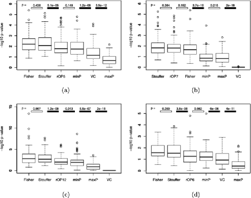
Figure 2: Comparison of different meta-analysis methods using pathway analysis. (a) Brain cancer. (b) MDD. (c) Diabetes. (d) Brain cancer and 1 random MDD.

Table 2 showed the number of detected DE genes under FDR${}=5\%$. We can immediately observe that Fisher and Stouffer generally detected many more biomarkers because they targeted on $\mathrm{HS}_{B}$ (genes differentially expressed in one or more studies). Although minP also targeted on $\mathrm{HS}_{B}$, it sometimes detected extremely small numbers of DE genes in weak-signal data such as the MDD and diabetes examples. This is reasonable because minP has very weak power to detect consistent but weak signals across studies [e.g., $p$-values${}=(0.1,0.1,\ldots,0.1)$]. The stringent maxP method detected few numbers of DE genes in general. Vote counting detected very few genes especially when the effect sizes were moderate (in the MDD and diabetes examples). rOP detected more DE genes than maxP because of its relaxed $\mathrm{HS}_{r}$ hypothesis setting. It identified about 50–65% fewer DE genes than Fisher’s and Stouffer’s methods, but guaranteed that the genes detected were differentially expressed in the majority of the studies. We also performed the one-sided corrected rOP for comparison. This method detected similar numbers of DE genes compared to two-sided rOP, and the majority of detected DE genes in two-sided and one-sided rOP were overlapped in the brain cancer example. The result showed that almost all DE genes detected by two-sided rOP had a consistent fold-change direction across studies. In MDD, the one-sided rOP detected much fewer genes than the two-sided method. This implied that many genes related to MDD acted differently in different brain regions and in different cohorts.

Figure 2 showed the results of biological association from pathway analysis that were similarly shown in Figure 1(b). The result showed that the DE gene lists generated by Fisher and Stouffer were more associated with biological pathways. The rOP method generally performed better than maxP and minP and had similar biological association performance to Fisher’s and Stouffer’s methods.

4 Statistical properties of rOP

4.1 Power calculation of rOP and asymptotic properties

When $K$ studies are combined, suppose $r_{0}$ of the $K$ studies have equal nonzero effect sizes and the rest of the ($K-r_{0}$) studies have zero effect sizes. That is,

$$H_{0}\dvtx\theta_{1} = \cdots=\theta_{K}=0,$$

$$H_{a}\dvtx\theta_{1} = \cdots=\theta_{r_{0}}=\theta\neq 0,\qquad\theta_{r_{0}+1}=\cdots=\theta_{K}=0.$$

For a single study, the power function given effect size $\theta$ is known as $\Pr(p_{i}\leq\alpha_{0}|\theta)$. We will derive the statistical power of rOP under this simplified hypothesis setting when $r_{0}$ and $r$ for rOP are given. Under $H_{0}$, the rejection threshold for the rOP statistic is $\beta=B_{\alpha}(r,K-r+1)$ (the $\alpha$ quantile of a beta distribution with shape parameters $r$ and $K-r+1$), where the significance level of the meta-analysis is set at $\alpha$. The power of rejection threshold $\beta$ under $H_{a}$ is $\Pr(p_{(r)}\leq\beta|H_{a})=\Pr(\sum_{i=1}^{K}I(p_{i}\leq\beta)\geq r|H_{a})$. By definition, $\Pr(p_{i}\leq\beta|\theta_{i}=0)=\beta$ and we further denote $\beta^{\prime}=\Pr(p_{i}\leq\beta|\theta_{i}=\theta)$. The power calculation of interest is equivalent to finding the probabilities of having at least $r$ successes in $K$ independent Bernoulli trials, among which $r_{0}$ have success probabilities $\beta^{\prime}$, and $K-r_{0}$ have success probabilities $\beta$:

$$\Pr(p_{(r)}\leq\beta|H_{a}) = \sum_{i=r}^{K}\sum_{j=\max(0,i-K+r_{0})}^{\min(i,r_{0})}\pmatrix{r_{0}\cr j}\beta^{\prime j}\bigl{(}1-\beta^{\prime}\bigr{)}^{r_{0}-j}$$

$$\hskip 84.0pt{}\times\pmatrix{K-r_{0}\cr i-j}\beta^{i-j}(1-\beta)^{K-r_{0}-i+j}.$$

Remark 4.

We note that the assumption of $r_{0}$ equal nonzero effect sizes can be relaxed. When the nonzero effects are not equal, the power calculation can be done in polynomial time using dynamic programming.

Below we demonstrate some asymptotic properties of rOP.

Theorem 4.1

Assume $r_{0}$ is fixed. When the effect size $\theta$ and $K$ are fixed and the sample size of study $k$ $N_{k}\rightarrow\infty$, $\Pr(p_{(r)}\leq\beta|H_{a})\rightarrow 1$ if $r\leq r_{0}$. When $r>r_{0}$, $\Pr(p_{(r)}\leq\beta|H_{a})\rightarrow c(r)<1$ and $c(r)$ is a decreasing function in $r$.

When $N_{k}\rightarrow\infty$, $\beta^{\prime}\rightarrow 1$. The theorem easily follows from the power calculation formulae. Theorem 4.1 states that, asymptotically, if the parameter $r$ in rOP is specified less or equal to the true $r_{0}$, the statistical power converges to 1 as intuitively expected. When specifying $r$ greater than $r_{0}$, the statistical power is weakened with increasing $r$. Particularly, maxP will have weak power. In contrast to Theorem 4.1, for methods designed for $\mathrm{HS}_{B}$ (e.g., Fisher’s method, Stouffer’s method and minP), the power always converges to 1 if $N_{k}\rightarrow\infty$ and $r_{0}>0$. Figure 3(a) shows the power curve of rOP for different $r$ when $K=10$, $r_{0}=6$ and $N_{k}\rightarrow\infty$.

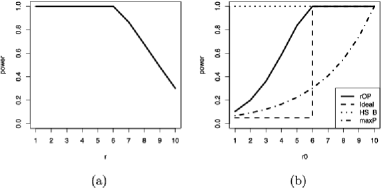
Figure 3: Power of rOP method when $N_{k}\rightarrow\infty$, $K=10$. (a) $r_{0}=6$, $r=1$–10. (b) $r=6$, $r_{0}=0$–10.

Lemma 4.1

Assume the parameter $r$ used in rOP is fixed. When the effect size $\theta$ and $K$ are fixed and the sample sizes $N_{k}\rightarrow\infty$, $\Pr(p_{(r)}\leq\beta|H_{a})\rightarrow 1$ if $r_{0}\geq r$. When $r_{0}<r$, $\Pr(p_{(r)}\leq\beta|H_{a})\rightarrow c(r_{0})<1$ and $c(r_{0})$ is an increasing function in $r_{0}$.

Lemma 4.1 takes a different angle from Theorem 4.1. When the parameter $r$ used in rOP is fixed, it asymptotically has perfect power to detect all genes that are differentially expressed in $r$ or more studies. It then does not have strong power to detect genes that are differentially expressed in less than $r$ studies. Figure 3(b) shows a power curve of rOP for $K=10$, $r=6$ and $N_{k}\rightarrow\infty$ (solid line). We note that the dashed line [$f(r)=0$ when $0\leq r_{0}<6$ and $f(r)=1$ when $6\leq r_{0}\leq 10$] is the ideal power curve for $\mathrm{HS}_{r}$ (i.e., it detects all genes that are differentially expressed in $r$ or more studies but does not detect any genes that are differentially expressed in less than $r$ studies). Methods like Fisher, Stouffer and minP target on $\mathrm{HS}_{B}$ and their power is always 1 asymptotically when $r_{0}>0$. The maxP method has perfect asymptotic power when $r_{0}=K=10$ but has relatively weak power when $r_{0}<K$. The rOP method lies between maxP and the methods designed for $\mathrm{HS}_{B}$. The power of rOP for $r_{0}\geq 6$ converges to 1, and for $r_{0}\leq 5$, the power is always smaller than 1 as the sample sizes in single studies go to infinity. Although the asymptotic powers of rOP for $r_{0}=4$ and $r_{0}=5$ are not too small, we are less concerned about these genes because they are still very likely to be important biomarkers.

4.2 Power comparison in simulated studies

To evaluate the performance of rOP in the genomic setting, we simulated a data set using the following procedure.

Step I.

Sample 200 gene clusters, with 20 genes in each and another 6000 genes that do not belong to any cluster. Denote $C_{g}\in\{0,1,2,\ldots,200\}$ as the cluster membership of gene $g$, where $C_{g}=0$ means that gene $g$ is not in a gene cluster.

Step II.

Sample the covariance matrix $\Sigma_{ck}$ for genes in cluster $c$ and in study $k$, where $1\leq c\leq 200$ and $1\leq k\leq 10$. First, sample $\Sigma^{\prime}_{ck}\sim W^{-1}(\Psi,60)$, where $\Psi=0.5I_{20\times 20}+0.5J_{20\times 20}$, $W^{-1}$ denotes the inverse Wishart distribution, $I$ is the identity matrix and $J$ is the matrix with all the elements equal 1. Then $\Sigma_{ck}$ is calculated by standardizing $\Sigma^{\prime}_{ck}$ such that the diagonal elements are all 1’s.

Step III.

Denote $g_{c1},\ldots,g_{c20}$ as the indices for the 20 genes in cluster $c$, that is, $C_{g_{cj}}=c$, where $1\leq c\leq 200$ and $1\leq j\leq 20$. Assuming the effect sizes are all zeros, sample gene expression levels of genes in cluster $c$ for sample $n$ as $(X^{\prime}_{g_{c1}nk},\ldots,X^{\prime}_{g_{c20}nk})^{T}\sim\mathit{MVN}(0,\Sigma_{ck})$, where $1\leq n\leq 100$ and $1\leq k\leq 10$, and sample expression level for gene $g$ which is not in a cluster (i.e., $C_{g}=0$) for sample $n$ as $X^{\prime}_{gnk}\sim N(0,1)$, where $1\leq n\leq 100$ and $1\leq k\leq 10$.

Step IV.

Sample the true number of studies that gene $g$ is DE, $t_{g}$, from a discrete uniform distribution that takes values on $1,2,\ldots,10$, for $1\leq g\leq 1000$; and set $t_{g}=0$ for $1001\leq g\leq{}$10,000.

Step V.

Sample $\delta_{gk}$, which indicates whether gene $g$ is DE in study $k$, from a discrete uniform distribution that takes values on 0 or 1 and with the constraint that $\sum_{k}\delta_{gk}=t_{g}$, where $1\leq g\leq 1000$ and $1\leq k\leq 10$. For $1001\leq g\leq{}$10,000 and $1\leq k\leq 10$, set $\delta_{gk}=0$.

Step VI.

Sample the effect size $\mu_{gk}$ uniformly from $[-1,-0.5]\cup[0.5,1]$. For control samples, set the expression levels as $X_{gnk}=X^{\prime}_{gnk}$; for case samples, set the expression levels as $Y_{gnk}=X^{\prime}_{g(n+50)k}+\mu_{gk}\cdot\delta_{gk}$, for $1\leq g\leq{}$10,000, $1\leq n\leq 50$ and $1\leq k\leq 10$.

Table 3: Mean FDRs for different methods in $\mathrm{HS}_{r}$ with $r=6$ by simulation analysis with correlated genes. The standard deviations of the FDRs in using 100 simulations are shown in the parentheses

	$\mathbf{FDR_{1}}$	$\mathbf{FDR_{2}}$	# of detected genes
rOP ($r=6$, PA)	0.0439 ($\pm$ 0.0106)	0.1818 ($\pm$ 0.0179)	620.16
rOP ($r=6$, BH)	0.0472 ($\pm$ 0.0094)	0.2029 ($\pm$ 0.0184)	617.53
rOP ($r=6$, BY)	0.0043 ($\pm$ 0.0031)	0.1044 ($\pm$ 0.0139)	539.85
Fisher	0.0441 ($\pm$ 0.0090)	0.4186 ($\pm$ 0.0212)	934.91
Stouffer	0.0440 ($\pm$ 0.0089)	0.3623 ($\pm$ 0.0217)	858.86
minP	0.0466 ($\pm$ 0.0103)	0.4567 ($\pm$ 0.0207)	958.26
maxP	0.0459 ($\pm$ 0.0199)	0.0729 ($\pm$ 0.0251)	201.02
Vote counting	0.0000 ($\pm$ 0.0000)	0.0003 ($\pm$ 0.0016)	234.43

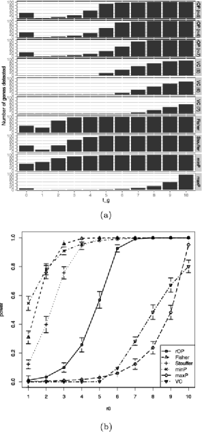
Figure 4: Simulation results for rOP and other methods with correlated genes. (a) Number of genes detected by difference methods. The detected genes are binned according to their $t_{g}$’s. (b) Power of different methods for genes with $r_{0}$ nonzero effect sizes.

In the simulated data set, 10 studies with 10,000 genes were simulated. Within each study, there were 50 cases and 50 controls. The first 1000 genes were DE in 1 to 10 studies with equal probabilities; and the rest of the 9000 genes were DE in none of the studies. We denoted $t_{g}$ as the true number of studies where gene $g$ was DE. To mimic the gene dependencies in a real gene expression data set, within the 10,000 genes, we drew 200 gene clusters with 20 genes in each. We sampled the data such that the genes within the same cluster were correlated. The correlation matrices for different studies and different gene clusters were sampled from an inverse Wishart distribution. Suppose the goal of the meta-analysis was to obtain biomarkers differentially expressed in at least 60% (6 out of 10) of the studies (i.e., $\mathrm{HS}_{r}$ with $r=6$). We performed two sample $t$-tests in each study and combined the $p$-values using rOP with $r=6$. $\mathrm{FDR}\leq 5\%$ was controlled using the permutation analysis. To compare rOP with other methods in the $\mathrm{HS}_{r}$ setting, we defined two FDR criteria as follows. Note that $\mathrm{FDR}_{1}$ targets on $H_{0}\dvtx t_{g}=0$ and $\mathrm{FDR}_{2}$ targets on $H_{0}\dvtx t_{g}<r$:

$$\mathrm{FDR}_{1} = \frac{\sum_{g}I(t_{g}=0\mbox{ and gene $g$ is detected})}{\#\{\mbox{genes detected}\}},$$

$$\mathrm{FDR}_{2} = \frac{\sum_{g}I(t_{g}<r\mbox{ and gene $g$ is detected})}{\#\{\mbox{genes detected}\}}.$$

Table 3 listed the average $\mathrm{FDR}_{1}$ and $\mathrm{FDR}_{2}$ for different methods calculated using 100 simulations. We can see that although $\mathrm{FDR}_{1}$ was well controlled, all the methods were anti-conservative in terms of $\mathrm{FDR}_{2}$, since the inference of the five methods was based on $H_{0}\dvtx t_{g}=0$ while genes with $1\leq t_{g}\leq 5$ existed and were calculated toward $\mathrm{FDR}_{2}$. To compare different FDR control methods, we also included the results of the Benjamini–Hochberg and Benjamini–Yekutieli procedures. According to the simulation, the Benjamini–Hochberg procedure controlled FDR similarly to the permutation test. The Benjamini–Yekutieli procedure, on the other hand, was too conservative that the $\mathrm{FDR}_{1}$ was controlled at about $1/10$ of the nominal FDR level. Figure 4 showed the number of detected DE genes and the statistical power of different methods for genes with $t_{g}$ from 1 to 10. From Figure 4(a), we noticed that Fisher, Stouffer and minP methods detected many genes with $1\leq t_{g}\leq 5$, which violated our targeted $\mathrm{HS}_{r}$ with $r=6$. MaxP detected very few genes and missed many targeted markers with $6\leq t_{g}\leq 9$. Only rOP generated the result most compatible with $\mathrm{HS}_{r}$ ($r=6$). Most genes with $6\leq t_{g}\leq 10$ were detected. The high $\mathrm{FDR}_{2}=18.2\%$ mostly came from genes with $4\leq t_{g}\leq 5$, genes that were very likely important markers and were minor mistakes. Vote counting detected genes with $t_{g}\geq 6$ but was less powerful. The relationship of vote counting and rOP will be further discussed in Section 4.3. We also performed rOP ($r=5$) and rOP ($r=7$) to compare the robustness of slightly different selections of $r$. Among the 620.16 DE genes (averaged over 100 simulations) detected by rOP ($r=6$), 594.15 (95.8%) of them were also detected by rOP ($r=5$) and 516.28 (83.3%) of them were also detected by rOP ($r=7$). The result of Figure 4(b) was consistent with the theoretical power calculation as shown in Figure 3(b).

We also performed the simulation without correlated genes. The results were shown in the supplement Table 2 [Song and Tseng (2014c)] and supplement Figure 6 [Song and Tseng (2014d)]. We noticed that the FDRs were controlled well in both correlated and uncorrelated cases. However, the standard deviations of FDRs with correlated genes were higher than the FDRs with only independent genes, which indicated some instability of the FDR control with correlated genes reported by Qiu, Yakovlev et al. (2006).

4.3 Connection with vote counting

Vote counting has been used in many meta-analysis applications due to its simplicity, while it has been criticized as being problematic and statistically inefficient. Hedges and Olkin (1980) showed that the power of vote counting converges to 0 when many studies of moderate effect sizes are combined (see supplement Theorem 1 [Song and Tseng (2014b)]). We, however, surprisingly found that rOP has a close connection with vote counting, and rOP can be viewed as a generalized vote counting with better statistical properties. There are many variations of vote counting in the literature. One popular approach is to count the number of studies that have $p$-values smaller than a prespecified threshold, $\alpha$. We define this quantity as

$$r=f(\alpha)=\sum_{k=1}^{K}I\{p_{k}<\alpha\}$$ (1)

and define its related proportion as $\pi=E(r)/K$. The test hypothesis is

$$\cases{H_{0}\dvtx\pi=\pi_{0},\vspace*{2pt}\cr H_{a}\dvtx\pi>\pi_{0},}$$

where $\pi_{0}=0.5$ is often used in the applications. Under the null hypothesis, $r\sim\mathit{BIN}(K,\alpha)$ and $\pi=\alpha$, so the rejection region can be established. In the vote counting procedure, $\alpha$ and $\pi_{0}$ are two preset parameters and the inference is made on the test statistic $r$.

In the rOP method, we view equation (1) from another direction. We can easily show that if we solve equation (1) to obtain $\alpha=f^{-1}(r)$, the solution will be $\alpha\in[p_{(r)},p_{(r+1)})$, and one may choose $\alpha=p_{(r)}$ as the solution. In other words, rOP presets $r$ as a given parameter, and the inference is based on the test statistic $\alpha=p_{(r)}$.

It is widely criticized that vote counting is powerless because when the effect sizes are moderate and the power of single studies is lower than $\pi_{0}$, as $K$ increases, the percentage of significant studies will converge to the single study power. However, in the rOP method, because the $r$th quantile is used, tests of the top $r$ studies are combined, which helps the rejection probability of rOP achieve 1 as $K\rightarrow\infty$. It should be noted that the major difference between rOP and vote counting is that the test statistic $\alpha=p_{(r)}$ in rOP increases as $K$ and $r=K\cdot c$ increase, which keeps information of the $r$ smallest $p$-values. On the contrary, for vote counting, $\alpha$ is often chosen small and fixed when $K$ increases. In supplement Theorem 1 [Song and Tseng (2014b)], the power of vote counting converges to 0 as $K\rightarrow\infty$, while the power of rOP converges to 1 asymptotically as proved in supplement Theorem 2 [Song and Tseng (2014b)].

5 Conclusion

In this paper we proposed a general class of order statistics of $p$-values, called $r$th ordered $p$-value (rOP), for genomic meta-analysis. This family of statistics included the traditional maximum $p$-value (maxP) and minimum $p$-value (minP) statistics that target on DE genes in “all studies” ($\mathrm{HS}_{A}$) or “one or more studies” ($\mathrm{HS}_{B}$). We extended $\mathrm{HS}_{A}$ to a robust form that detected DE genes “in the majority of studies” ($\mathrm{HS}_{r}$) and developed the rOP method for this purpose. The new robust hypothesis setting has an intuitive interpretation and is more adequate in genomic applications where unexpected noise is common in the data. We developed the algorithm of rOP for microarray meta-analysis and proposed two methods to estimate $r$ in real applications. Under “two-class” comparisons, we proposed a one-sided corrected form of rOP to avoid detection of discordant expression change across studies (i.e., significant up-regulation in some studies but down-regulation in other studies). Finally, we performed power analysis and examined asymptotic properties of rOP to demonstrate appropriateness of rOP for $\mathrm{HS}_{r}$ over existing methods such as Fisher, Stouffer, minP and maxP. We further showed a surprising connection between vote counting and rOP that rOP can be viewed as a generalized vote counting with better statistical property. Applications of rOP to three examples of brain cancer, major depressive disorder (MDD) and diabetes showed better performance of rOP over maxP in terms of detection power (number of detected markers) and biological association by pathway analysis.

There are two major limitations of rOP. First, rOP is for $\mathrm{HS}_{r}$, but the null and alternative hypotheses are not complementary (see Section 2.1). Thus, it has weaker ability to exclude markers that are differentially expressed in “less than $r$” studies since the null of $\mathrm{HS}_{r}$ is “differentially expressed in none of the studies.” One solution to improve the anti-conservative inference (which is also our future work) is by Bayesian modeling of $p$-values with a family of beta distributions [Erickson, Kim and Allison (2009)]. Second, selection of $r$ may not always be conclusive from the two methods we proposed; the external pathway information may especially be prone to errors and may not be informative to the data. But since choosing slightly different $r$ usually gives similar results, this is not a severe problem in most applications. We have tested a different approach by adaptively choosing the best gene-specific $r$ that generates the best $p$-value. The result is, however, not stable and the gene-specific parameter $r$ is hard to interpret in applications.

Although many meta-analysis methods have been proposed and applied to microarray applications, it is still not clear which method enjoys better performance under what condition. The selection of an adequate (or best) method heavily depends on the biological goal (as illustrated by the hypothesis settings in this paper) and the data structure. In this paper, we stated a robust hypothesis setting ($\mathrm{HS}_{r}$) that is commonly targeted in biological applications (i.e., identify markers statistically significant in the majority of studies) and developed an order statistic method (rOP) as a solution. The three applications covered “cleaner” data (brain cancer) to “noisier” data (complex genetics in MDD and diabetes), and rOP performed well in all three examples. We expect that the robust hypothesis setting and the order statistic methodology will find many more applications in genomic research and traditional univariate meta-analysis in the future.

For multiple comparison control, we propose to either apply the parametric beta null distribution to assess the $p$-value and perform the Benjamini–Hochberg (BH) procedure for $p$-value adjustment or conduct a conventional permutation analysis by permuting class labels in each study. The former approach is easy to implement, and the latter approach better preserves the gene correlation structure in the inference. Instead of the BH procedure, we also tested the Benjamini–Yekutieli (BY) procedure which is applicable to the general dependence structure but found that it is overly conservative for genomic applications. The problem of FDR control under general high-dimensional dependence structures is beyond the scope of this paper but is critical in applications and deserves future research.

Implementation of rOP is available in the “MetaDE” package in R together with over 12 microarray meta-analysis methods in the package.MetaDE has been integrated with other quality control methods [“MetaQC” package, Kang et al. (2012)] and pathway enrichment analysis methods [“MetaPath” package, Shen and Tseng (2010)]. The future plan is to integrate the three packages with other genomic meta-analysis tools into a “MetaOmics” software suite [Wang et al. (2012b)].

References

- Begum et al. (2012) {barticle}[pbm] \bauthor\bsnmBegum, \bfnmFerdouse\binitsF., \bauthor\bsnmGhosh, \bfnmDebashis\binitsD., \bauthor\bsnmTseng, \bfnmGeorge C.\binitsG. C. and \bauthor\bsnmFeingold, \bfnmEleanor\binitsE. (\byear2012). \btitleComprehensive literature review and statistical considerations for GWAS meta-analysis. \bjournalNucleic Acids Res. \bvolume40 \bpages3777–3784. \biddoi=10.1093/nar/gkr1255, issn=1362-4962, pii=gkr1255, pmcid=3351172, pmid=22241776 \bptokimsref\endbibitem
- Benjamini and Hochberg (1995) {barticle}[mr] \bauthor\bsnmBenjamini, \bfnmYoav\binitsY. and \bauthor\bsnmHochberg, \bfnmYosef\binitsY. (\byear1995). \btitleControlling the false discovery rate: A practical and powerful approach to multiple testing. \bjournalJ. R. Stat. Soc. Ser. B \bvolume57 \bpages289–300. \bidissn=0035-9246, mr=1325392 \bptokimsref\endbibitem
- Benjamini and Yekutieli (2001) {barticle}[mr] \bauthor\bsnmBenjamini, \bfnmYoav\binitsY. and \bauthor\bsnmYekutieli, \bfnmDaniel\binitsD. (\byear2001). \btitleThe control of the false discovery rate in multiple testing under dependency. \bjournalAnn. Statist. \bvolume29 \bpages1165–1188. \biddoi=10.1214/aos/1013699998, issn=0090-5364, mr=1869245 \bptokimsref\endbibitem
- Berger (1982) {barticle}[mr] \bauthor\bsnmBerger, \bfnmRoger L.\binitsR. L. (\byear1982). \btitleMultiparameter hypothesis testing and acceptance sampling. \bjournalTechnometrics \bvolume24 \bpages295–300. \biddoi=10.2307/1267823, issn=0040-1706, mr=0687187 \bptokimsref\endbibitem
- Berger and Hsu (1996) {barticle}[mr] \bauthor\bsnmBerger, \bfnmRoger L.\binitsR. L. and \bauthor\bsnmHsu, \bfnmJason C.\binitsJ. C. (\byear1996). \btitleBioequivalence trials, intersection-union tests and equivalence confidence sets. \bjournalStatist. Sci. \bvolume11 \bpages283–319. \biddoi=10.1214/ss/1032280304, issn=0883-4237, mr=1445984 \bptnotecheck related \bptokimsref\endbibitem
- Birnbaum (1954) {barticle}[mr] \bauthor\bsnmBirnbaum, \bfnmAllan\binitsA. (\byear1954). \btitleCombining independent tests of significance. \bjournalJ. Amer. Statist. Assoc. \bvolume49 \bpages559–574. \bidissn=0162-1459, mr=0065101 \bptokimsref\endbibitem
- Cooper, Hedges and Valentine (2009) {bbook}[author] \bauthor\bsnmCooper, \bfnmH. M.\binitsH. M., \bauthor\bsnmHedges, \bfnmL. V.\binitsL. V. and \bauthor\bsnmValentine, \bfnmJ. C.\binitsJ. C. (\byear2009). \btitleThe Handbook of Research Synthesis and Meta-Analysis. \bpublisherRussell Sage Foundation, \blocationThousand Oaks, CA. \bptokimsref\endbibitem
- Erickson, Kim and Allison (2009) {bbook}[author] \bauthor\bsnmErickson, \bfnmS.\binitsS., \bauthor\bsnmKim, \bfnmK.\binitsK. and \bauthor\bsnmAllison, \bfnmD. B.\binitsD. B. (\byear2009). \btitleMeta-Analysis and Combining Information in Genetics and Genomics. \bpublisherChapman & Hall/CRC, \blocationLondon. \bptokimsref\endbibitem
- Fisher (1925) {bbook}[author] \bauthor\bsnmFisher, \bfnmR. A.\binitsR. A. (\byear1925). \btitleStatistical Methods for Research Workers. \bpublisherOliver and Boyd, \blocationEdinburgh. \bptokimsref\endbibitem
- Hedges and Olkin (1980) {barticle}[author] \bauthor\bsnmHedges, \bfnmL. V.\binitsL. V. and \bauthor\bsnmOlkin, \bfnmI.\binitsI. (\byear1980). \btitleVote-counting methods in research synthesis. \bjournalPsychol. Bull. \bvolume88 \bpages359–369. \bptokimsref\endbibitem
- Kang et al. (2012) {barticle}[pbm] \bauthor\bsnmKang, \bfnmDongwan D.\binitsD. D., \bauthor\bsnmSibille, \bfnmEtienne\binitsE., \bauthor\bsnmKaminski, \bfnmNaftali\binitsN. and \bauthor\bsnmTseng, \bfnmGeorge C.\binitsG. C. (\byear2012). \btitleMetaQC: Objective quality control and inclusion/exclusion criteria for genomic meta-analysis. \bjournalNucleic Acids Res. \bvolume40 \bpagese15. \biddoi=10.1093/nar/gkr1071, issn=1362-4962, pii=gkr1071, pmcid=3258120, pmid=22116060 \bptokimsref\endbibitem
- Li and Tseng (2011) {barticle}[mr] \bauthor\bsnmLi, \bfnmJia\binitsJ. and \bauthor\bsnmTseng, \bfnmGeorge C.\binitsG. C. (\byear2011). \btitleAn adaptively weighted statistic for detecting differential gene expression when combining multiple transcriptomic studies. \bjournalAnn. Appl. Stat. \bvolume5 \bpages994–1019. \biddoi=10.1214/10-AOAS393, issn=1932-6157, mr=2840184 \bptokimsref\endbibitem
- Littell and Folks (1971) {barticle}[mr] \bauthor\bsnmLittell, \bfnmRamon C.\binitsR. C. and \bauthor\bsnmFolks, \bfnmJ. Leroy\binitsJ. L. (\byear1971). \btitleAsymptotic optimality of Fisher’s method of combining independent tests. \bjournalJ. Amer. Statist. Assoc. \bvolume66 \bpages802–806. \bidissn=0162-1459, mr=0312634 \bptokimsref\endbibitem
- Littell and Folks (1973) {barticle}[mr] \bauthor\bsnmLittell, \bfnmRamon C.\binitsR. C. and \bauthor\bsnmFolks, \bfnmJ. Leroy\binitsJ. L. (\byear1973). \btitleAsymptotic optimality of Fisher’s method of combining independent tests. II. \bjournalJ. Amer. Statist. Assoc. \bvolume68 \bpages193–194. \bidissn=0162-1459, mr=0375577 \bptokimsref\endbibitem
- Owen (2009) {barticle}[mr] \bauthor\bsnmOwen, \bfnmArt B.\binitsA. B. (\byear2009). \btitleKarl Pearson’s meta-analysis revisited. \bjournalAnn. Statist. \bvolume37 \bpages3867–3892. \biddoi=10.1214/09-AOS697, issn=0090-5364, mr=2572446 \bptokimsref\endbibitem
- Park et al. (2009) {barticle}[pbm] \bauthor\bsnmPark, \bfnmPeter J.\binitsP. J., \bauthor\bsnmKong, \bfnmSek Won\binitsS. W., \bauthor\bsnmTebaldi, \bfnmToma\binitsT., \bauthor\bsnmLai, \bfnmWeil R.\binitsW. R., \bauthor\bsnmKasif, \bfnmSimon\binitsS. and \bauthor\bsnmKohane, \bfnmIsaac S.\binitsI. S. (\byear2009). \btitleIntegration of heterogeneous expression data sets extends the role of the retinol pathway in diabetes and insulin resistance. \bjournalBioinformatics \bvolume25 \bpages3121–3127. \biddoi=10.1093/bioinformatics/btp559, issn=1367-4811, pii=btp559, pmcid=2778339, pmid=19786482 \bptokimsref\endbibitem
- Pearson (1934) {barticle}[author] \bauthor\bsnmPearson, \bfnmK.\binitsK. (\byear1934). \btitleOn a new method of determining “goodness of fit.” \bjournalBiometrika \bvolume26 \bpages425–442. \bptokimsref\endbibitem
- Qiu, Yakovlev et al. (2006) {barticle}[author] \bauthor\bsnmQiu, \bfnmX.\binitsX., \bauthor\bsnmYakovlev, \bfnmA.\binitsA. \betalet al. (\byear2006). \btitleSome comments on instability of false discovery rate estimation. \bjournalJ. Bioinform. Comput. Biol. \bvolume4 \bpages1057–1068. \bptokimsref\endbibitem
- Rhodes et al. (2002) {barticle}[pbm] \bauthor\bsnmRhodes, \bfnmDaniel R.\binitsD. R., \bauthor\bsnmBarrette, \bfnmTerrence R.\binitsT. R., \bauthor\bsnmRubin, \bfnmMark A.\binitsM. A., \bauthor\bsnmGhosh, \bfnmDebashis\binitsD. and \bauthor\bsnmChinnaiyan, \bfnmArul M.\binitsA. M. (\byear2002). \btitleMeta-analysis of microarrays: Interstudy validation of gene expression profiles reveals pathway dysregulation in prostate cancer. \bjournalCancer Res. \bvolume62 \bpages4427–4433. \bidissn=0008-5472, pmid=12154050 \bptokimsref\endbibitem
- Roy (1953) {barticle}[mr] \bauthor\bsnmRoy, \bfnmS. N.\binitsS. N. (\byear1953). \btitleOn a heuristic method of test construction and its use in multivariate analysis. \bjournalAnn. Math. Stat. \bvolume24 \bpages220–238. \bidissn=0003-4851, mr=0057519 \bptokimsref\endbibitem
- Shen and Tseng (2010) {barticle}[pbm] \bauthor\bsnmShen, \bfnmKui\binitsK. and \bauthor\bsnmTseng, \bfnmGeorge C.\binitsG. C. (\byear2010). \btitleMeta-analysis for pathway enrichment analysis when combining multiple genomic studies. \bjournalBioinformatics \bvolume26 \bpages1316–1323. \biddoi=10.1093/bioinformatics/btq148, issn=1367-4811, pii=btq148, pmcid=2865865, pmid=20410053 \bptokimsref\endbibitem
- Song and Tseng (2014a) {bmisc}[auto] \bauthor\bsnmSong, \bfnmChi\binitsC. and \bauthor\bsnmTseng, \bfnmGeorge C.\binitsG. C. (\byear2014a). \bhowpublishedSupplement to “Hypothesis setting and order statistic for robust genomic meta-analysis.” DOI:\doiurl10.1214/13-AOAS683SUPPA. \bptokimsref \endbibitem
- Song and Tseng (2014b) {bmisc}[auto] \bauthor\bsnmSong, \bfnmChi\binitsC. and \bauthor\bsnmTseng, \bfnmGeorge C.\binitsG. C. (\byear2014b). \bhowpublishedSupplement to “Hypothesis setting and order statistic for robust genomic meta-analysis.” DOI:\doiurl10.1214/13-AOAS683SUPPB. \bptokimsref \endbibitem
- Song and Tseng (2014c) {bmisc}[auto] \bauthor\bsnmSong, \bfnmChi\binitsC. and \bauthor\bsnmTseng, \bfnmGeorge C.\binitsG. C. (\byear2014c). \bhowpublishedSupplement to “Hypothesis setting and order statistic for robust genomic meta-analysis.” DOI:\doiurl10.1214/13-AOAS683SUPPC. \bptokimsref \endbibitem
- Song and Tseng (2014d) {bmisc}[auto] \bauthor\bsnmSong, \bfnmChi\binitsC. and \bauthor\bsnmTseng, \bfnmGeorge C.\binitsG. C. (\byear2014d). \bhowpublishedSupplement to “Hypothesis setting and order statistic for robust genomic meta-analysis.” DOI:\doiurl10.1214/13-AOAS683SUPPD. \bptokimsref \endbibitem
- Stouffer et al. (1949) {bbook}[author] \bauthor\bsnmStouffer, \bfnmS. A.\binitsS. A., \bauthor\bsnmSuchman, \bfnmE. A.\binitsE. A., \bauthor\bsnmDevinney, \bfnmL. C.\binitsL. C., \bauthor\bsnmStar, \bfnmS. A.\binitsS. A. and \bauthor\bsnmWilliams Jr., \bfnmR. M.\binitsR. M. (\byear1949). \btitleThe American Soldier: Adjustment During Army Life. \bpublisherPrinceton Univ. Press, \blocationPrinceton, NJ. \bptokimsref\endbibitem
- Subramanian et al. (2005) {barticle}[author] \bauthor\bsnmSubramanian, \bfnmA.\binitsA., \bauthor\bsnmTamayo, \bfnmP.\binitsP., \bauthor\bsnmMootha, \bfnmV. K.\binitsV. K., \bauthor\bsnmMukherjee, \bfnmS.\binitsS., \bauthor\bsnmEbert, \bfnmB. L.\binitsB. L., \bauthor\bsnmGillette, \bfnmM. A.\binitsM. A., \bauthor\bsnmPaulovich, \bfnmA.\binitsA., \bauthor\bsnmPomeroy, \bfnmS. L.\binitsS. L., \bauthor\bsnmGolub, \bfnmT. R.\binitsT. R., \bauthor\bsnmLander, \bfnmE. S.\binitsE. S. \betalet al. (\byear2005). \btitleGene set enrichment analysis: A knowledge-based approach for interpreting genome-wide expression profiles. \bjournalProc. Natl. Acad. Sci. USA \bvolume102 \bpages15545–15550. \bptokimsref\endbibitem
- Tibshirani, Walther and Hastie (2001) {barticle}[mr] \bauthor\bsnmTibshirani, \bfnmRobert\binitsR., \bauthor\bsnmWalther, \bfnmGuenther\binitsG. and \bauthor\bsnmHastie, \bfnmTrevor\binitsT. (\byear2001). \btitleEstimating the number of clusters in a data set via the gap statistic. \bjournalJ. R. Stat. Soc. Ser. B Stat. Methodol. \bvolume63 \bpages411–423. \biddoi=10.1111/1467-9868.00293, issn=1369-7412, mr=1841503 \bptokimsref\endbibitem
- Tippett (1931) {bbook}[author] \bauthor\bsnmTippett, \bfnmL. H. C.\binitsL. H. C. (\byear1931). \btitleThe Methods of Statistics. \bpublisherWilliams Norgate, \blocationLondon. \bptokimsref\endbibitem
- Tseng, Ghosh and Feingold (2012) {barticle}[pbm] \bauthor\bsnmTseng, \bfnmGeorge C.\binitsG. C., \bauthor\bsnmGhosh, \bfnmDebashis\binitsD. and \bauthor\bsnmFeingold, \bfnmEleanor\binitsE. (\byear2012). \btitleComprehensive literature review and statistical considerations for microarray meta-analysis. \bjournalNucleic Acids Res. \bvolume40 \bpages3785–3799. \biddoi=10.1093/nar/gkr1265, issn=1362-4962, pii=gkr1265, pmcid=3351145, pmid=22262733 \bptokimsref\endbibitem
- Wang et al. (2012a) {barticle}[pbm] \bauthor\bsnmWang, \bfnmXingbin\binitsX., \bauthor\bsnmLin, \bfnmYan\binitsY., \bauthor\bsnmSong, \bfnmChi\binitsC., \bauthor\bsnmSibille, \bfnmEtienne\binitsE. and \bauthor\bsnmTseng, \bfnmGeorge C.\binitsG. C. (\byear2012a). \btitleDetecting disease-associated genes with confounding variable adjustment and the impact on genomic meta-analysis: With application to major depressive disorder. \bjournalBMC Bioinformatics \bvolume13 \bpages52. \biddoi=10.1186/1471-2105-13-52, issn=1471-2105, pii=1471-2105-13-52, pmcid=3342232, pmid=22458711 \bptokimsref\endbibitem
- Wang et al. (2012b) {barticle}[author] \bauthor\bsnmWang, \bfnmX.\binitsX., \bauthor\bsnmKang, \bfnmD. D.\binitsD. D., \bauthor\bsnmShen, \bfnmK.\binitsK., \bauthor\bsnmSong, \bfnmC.\binitsC., \bauthor\bsnmLu, \bfnmS.\binitsS., \bauthor\bsnmChang, \bfnmL. C.\binitsL. C., \bauthor\bsnmLiao, \bfnmS. G.\binitsS. G., \bauthor\bsnmHuo, \bfnmZ.\binitsZ., \bauthor\bsnmTang, \bfnmS.\binitsS., \bauthor\bsnmKaminski, \bfnmN.\binitsN. \betalet al. (\byear2012b). \btitleAn R package suite for microarray meta-analysis in quality control, differentially expressed gene analysis and pathway enrichment detection. \bjournalBioinformatics \bvolume28 \bpages2534–2536. \bptokimsref\endbibitem
- Wilkinson (1951) {barticle}[pbm] \bauthor\bsnmWilkinson, \bfnmB.\binitsB. (\byear1951). \btitleA statistical consideration in psychological research. \bjournalPsychol. Bull. \bvolume48 \bpages156–158. \bidissn=0033-2909, pmid=14834286 \bptokimsref\endbibitem