Detection boundary and Higher Criticism approach for rare and weak genetic effects

Abstract

Genome-wide association studies (GWAS) have identified many genetic factors underlying complex human traits. However, these factors have explained only a small fraction of these traits’ genetic heritability. It is argued that many more genetic factors remain undiscovered. These genetic factors likely are weakly associated at the population level and sparsely distributed across the genome. In this paper, we adapt the recent innovations on Tukey’s Higher Criticism (Tukey [The Higher Criticism (1976) Princeton Univ.]; Donoho and Jin [Ann. Statist. 32 (2004) 962–994]) to SNP-set analysis of GWAS, and develop a new theoretical framework in large-scale inference to assess the joint significance of such rare and weak effects for a quantitative trait. In the core of our theory is the so-called detection boundary, a curve in the two-dimensional phase space that quantifies the rarity and strength of genetic effects. Above the detection boundary, the overall effects of genetic factors are strong enough for reliable detection. Below the detection boundary, the genetic factors are simply too rare and too weak for reliable detection. We show that the HC-type methods are optimal in that they reliably yield detection once the parameters of the genetic effects fall above the detection boundary and that many commonly used SNP-set methods are suboptimal. The superior performance of the HC-type approach is demonstrated through simulations and the analysis of a GWAS data set of Crohn’s disease.

, , , , and

1 Introduction

Genome-wide association studies (GWAS) aim to detect associated genetic factors by scanning up to several million genetic variants over the whole genome. Although many genetic factors have been successfully identified for human diseases, genes discovered to date account for only a small proportion of overall genetic contribution to many complex traits [Kraft and Hunter (2009), McCarthy et al. (2008)]. The remaining genetic factors to be detected likely have weak associations at the population level and are relatively rare among the huge number of candidates in the whole genome [Goldstein (2009), Wade (2009)]. Besides the efforts to increase sample size and improve disease classification, it is desirable to develop statistical methods that more effectively detect these rare and weak genetic signals not yet discovered.

Two types of statistical association methods are commonly used to analyze GWAS data: (1) single-SNP methods that analyze the associations between a trait and individual SNPs, and (2) SNP-set methods that study the associations between a trait and sets of SNPs. SNP-set methods were expected to be more promising than single-SNP methods from a biological perspective. Since multiple SNPs within the same gene, pathway or other physical and functional genomic segment could jointly affect disease risk, joint analysis of a set of such SNPs may better reveal the underlying mechanisms of complex traits than individual SNPs do. In the past years, many SNP-set methods have been proposed [Ballard, Cho and Zhao (2010), Hoh and Ott (2003), Hoh, Wille and Ott (2001), Li et al. (2009), Luo et al. (2010), Mukhopadhyay et al. (2010), Peng et al. (2009), Wang and Abbott (2008), Wang, Li and Bucan (2007), Yang, Hsieh and Fann (2008)]. Despite the encouraging progress in the literature, there lacks a statistical foundation for when and why the SNP-set methods would outperform single-SNP methods. In fact, some SNP-set methods are not automatically better, as we will show in this paper. At the same time, it is critical to know the limit of any statistical association methods, as well as the “best” of the methods, especially when genetic effects are rare and weak.

In this paper, we approach these problems from a statistical perspective. For a set of $L$ SNPs of $n$ individuals, we consider an additive genetic model

$$\mathbf{Y}=\beta_{0}+\beta_{1}\mathbf{X}_{1}+\beta_{2}\mathbf{X}_{2}+\cdots+\beta_{L}\mathbf{X}_{L}+\bolds{\varepsilon},$$ (1)

that is frequently used in GWAS [Kraft and Hunter (2009)]. The linear model is likely an oversimplification but we develop our ideas for this one first. See further comments in Section 7. Here $\mathbf{Y}=(Y_{1},\ldots,Y_{n})^{\prime}$ is the trait vector, and $\mathbf{X}_{j}=(X_{1j},\ldots,X_{nj})^{\prime}$ is the genotype vector of the $j$th SNP, $1\leq j\leq L$. The error term $\bolds{\varepsilon}=(\varepsilon_{1},\ldots,\varepsilon_{n})^{\prime}\sim N(\mathbf{0},\sigma^{2}\mathbf{I})$ is independent of the genotypes and can be used to represent other genetic and environmental variations [Falconer, Mackay and Frankham (1996)]. The variance parameter $\sigma^{2}$ is usually unknown and needs to be estimated. The coefficient vector $\beta=(\beta_{1},\beta_{2},\ldots,\beta_{L})^{\prime}$ is unknown to us, but is presumably rare in the sense that only a few of the coordinates of $\beta$ are nonzero. We call the $j$th coordinate of $\beta$ a “signal” if $\beta_{j}\neq 0$ and otherwise a “noise.” The term “rare signal” should not be confused with “rare genetic variation.” Signal rarity is the sparsity among features, but rare genetic variation is the sparsity among samples. In the literature, while signal rarity is well defined, signal weakness is a much more vague notion. As we will show below, signal weakness may result from weak genetic effect, small sample size and/or small genetic variation. Signal weakness is one of the main challenges in analyzing big data, such as GWAS data: The signals are generally very subtle and hard to find, and it is easy to be fooled.

Statistical literature on linear regression modeling has focused largely on the goal of separating the signals from the noise [Ayers and Cordell (2010), Guan and Stephens (2011), Hoggart et al. (2008), Wu et al. (2009), Xie, Cai and Li (2011)]. While this goal may provide a perfect solution, it is hard to reach due to a high demand for strong signals and is often not necessary in GWAS practice either. Thus, in this paper, we are primarily interested in the problem of signal detection, where the goal is to discover the associated SNP-sets rather than to identify the individually associated SNPs.

To understand why signal detection is important, from a statistics point of view it can be shown that given a rarity level of the signals there is a threshold effect on the signal strength. That is, signals falling under such a threshold cannot be separated from noise: for any procedure the sum of the number of signals that are misclassified as noises and the number of noises that are misclassified as signals cannot get substantially smaller than the number of signals. Nonetheless, in many cases while signal rarity and signal strength prohibit us to separate the signals from the noise, the numerous rare and weak effects can be combined and utilized in a meaningful way to solve many challenging problems including, but not limited to, signal detection, classification and clustering. This challenge has been successfully met, for example, in Donoho and Jin (2004, 2008), Jin and Wang (2013). From the genetics point of view, the signal detection problem is of major interest in the GWAS because the primary target of GWAS is to screen and allocate the informative genome regions, such as genes, which are more natural genomic functional units than individual SNPs. Furthermore, to validate associations, such positive regions will be further studied and individual SNP effects can still be discovered by refined and reliable experimental methods.

The signal detection problem in the model (1) can be reformulated as a joint hypothesis testing problem where $H_{0}$ is

$$H_{0}\dvtx\quad\beta_{j}=0,\qquad 1\leq j\leq L,$$

that is, no association exists between the trait and the SNP sets, against an alternative hypothesis $H_{1}$ that the trait is associated with a small fraction of SNPs in the sets

$$H_{1}\dvtx\quad\mbox{$\beta_{j}\neq 0$\qquad only for a small fraction of $j$, $1\leq j\leq L$}.$$

See Donoho and Jin (2004) for the subtlety of this problem, where the focus was on a Stein’s normal means model, which is much simpler than the model considered here.

Our study contains two key components: the detection boundary for signal detection and the statistic of Higher Criticism. We now discuss two components separately.

The detection boundary can be viewed as a way to address the fundamental capability and limit of SNP-set methods. In the two-dimensional phase space calibrating the signal rarity and signal strength, the detection boundary is a curve that separates the region of impossibility from the region of possibility. In the region of impossibility, the signals are so rare and weak that it is impossible to separate $H_{1}$ from $H_{0}$. That is, even for the most powerful method available, the signals are so rare and weak that it would have the sum of types I and II error rates to be almost $1$. In the region of possibility, it is possible to separate $H_{1}$ from $H_{0}$, and there exists a procedure whose sum of types I and II error rates is approximately $0$.

The study of the detection boundary has two merits. First, the detection boundary is provided as a function of the rarity and strength of genetic effects, the SNP-set size, the sample size, the error variance and the allele frequency, and thus simultaneously reveals the roles of these factors in gene-hunting. The result is applicable to genetic association studies of both common and rare genetic variants, the latter are the main target of finding the missing genetic factors using deep sequencing technologies [Ansorge (2009), Mardis (2008), Metzker (2010)]. Second, the detection boundary can serve as a benchmark for evaluating different SNP-set methods. In particular, note that any procedure will partition the aforementioned phase spaces into two regions: a region of possibility and a region of impossibility. We say a method achieves the optimal phase diagram if it partitions the two-dimensional phase space in exactly the same way as the optimal procedure does. As a result, for any procedure we can assess its optimality by investigating whether it achieves the optimal phase diagram.

Higher Criticism (HC) is a notion that goes back to Tukey (1976), and it was shown in Arias-Castro, Candès and Plan (2011), Donoho and Jin (2004), Hall and Jin (2008, 2010), Ingster, Tsybakov and Verzelen (2010) that HC is useful in detecting very rare and weak effects. However, these works deal with models different from the genetic model (1), and it is unclear whether the HC continues to behave well for the setting considered here. The genetic model is new in several aspects. First, the covariates are genotype data, rather than standardized or Gaussian variables. Second, the conditions for correlations among covariates, that is, the linkage disequilibrium structure, are better placed on the population correlations, rather than on the empirical correlations. Third, the error variance is realistically considered as unknown and needs to be estimated, rather than being assumed as known.

In this paper we adapt the HC to detect rare and weak genetic effects in a SNP-set analysis context. With substantial efforts, we work out the exact detection boundary associated with the genetic model (1). We propose a realistic HC procedure for analyzing real GWAS data and show that it achieves the optimal phase diagram in a rather broad context. We provide theoretical comparisons between HC and the several most commonly used SNP-set methods. Somewhat surprisingly, these well-known SNP-set methods do not achieve the optimal phase diagram for rare and weak signals. We further demonstrate the superiority of the HC-type methods with simulated data and real data.

The paper is organized as follows. In Section 2 we set up the genetic model and provide the detection boundary for rare and weak genetic effects. In Section 3 an HC procedure is proposed to reach the optimal detection boundary for rare and weak genetic signals. In Section 4 we discuss the connections of HC to False Discovery Rate (FDR) controlling methods. We show in Section 5 that some commonly used SNP-set based methods cannot reach the best detection boundary, and thus are not optimal. In Section 6 we compare various methods through numerical simulations and the analysis of a GWAS data of Crohn’s disease. In Section 7 we discuss relevant theoretical and practical issues. The proofs of the main theoretical results, the fundamental lemmas and their proofs, as well as the supplementary figures and tables, are given in the online supplementary material [Wu et al. (2014)].

2 Genetic model and detection boundary

In this section we characterize the detection boundary by introducing a theoretical framework.

We write in model (1)

$$\mathbf{X}_{j}=(X_{1j},X_{2j},\ldots,X_{nj})^{\prime},$$

so that $X_{kj}$ is the genotype of the $j$th SNP for the $k$th individual, where $1\leq j\leq L$, $1\leq k\leq n$. Let the minor allele $A_{j}$ of the $j$th SNP have a minor allele frequency (MAF) of $q_{j}$. We assume $q_{j}>q>0$, $1\leq j\leq L$, for some constant $q$. We use the copy number of minor alleles to code the SNP genotype, which follows a binomial distribution under the Hardy–Weinberg equilibrium (HWE) [Mendel (1866), Pearson (1904), Yulh (1902)]

$$X_{kj}\sim\operatorname{Binomial}(2,q_{j}).$$ (2)

In some genetic association studies, the individuals are assumed to be independent, that is, $X_{k_{1}j}$ and $X_{k_{2}l}$ are independent for any $k_{1}\neq k_{2}$. However, the dependency among SNPs, called linkage disequilibrium (LD), is a critical feature in GWAS data. We characterize the LD structure by the correlation matrix $\bolds{\Sigma}=\bolds{\Sigma}_{L\times L}$ among $X_{k1},\ldots,X_{kL}$. For $\gamma>0$ and $\Delta>0$, let

$$\mathcal{S}_{L}(\gamma,\Delta)=\{\bolds{\Sigma}\dvtx\mbox{each row of }\bolds{\Sigma}\mbox{ has no more than }$$

(3)

$$\hskip 62.0pt\Delta\mbox{ elements exceeding }\gamma\mbox{ in magnitude}\}.$$

With an appropriately small $\gamma$ and a moderately large $\Delta$, a matrix $\bolds{\Sigma}$ in $\mathcal{S}_{L}(\gamma,\Delta)$ can be interpreted as sparse, in the sense that each row of $\bolds{\Sigma}$ has relatively small coordinates. This setup has been studied in the theoretical statistics literature [Arias-Castro, Candès and Plan (2011)], and is relatively general and flexible for GWAS because the large correlations are allowed between SNPs far from each other. In Section 5 we will also consider another setup for $\bolds{\Sigma}$, where the correlation decays polynomially as the SNP distance increases.

We develop a theoretical framework where we use $L$ as the driving asymptotic parameter, and other parameters are tied to $L$ through fixed parameters. In particular, we model the sample size $n$ by

$$n=n_{L}=L^{a}\qquad\mbox{for some constant }a>0.$$ (4)

As $L$ grows to $\infty$, $n_{L}$ grows to $\infty$ as well. $n_{L}$ can be either larger than or smaller than $L$; both cases are common in recent GWAS.

Next, fixing $1/2<\alpha<1$ which we call the rarity parameter, we model the number of associated SNPs by

$$K=K_{L}=L^{1-\alpha},$$ (5)

so that the fraction of signals tends to $0$ as $L\rightarrow\infty$. In our calibrations, $K_{L}\ll\sqrt{L}$ and the signals are very rare. Seemingly, this is a very subtle situation. In contrast, the case $0<\alpha<1/2$ is both easier to analyze and less relevant to the major challenge of the genetic association study, so we omit the discussion on that. See, for example, Arias-Castro, Candès and Plan (2011), Donoho and Jin (2004).

At the same time, let $M^{\ast}\equiv\{j_{1},\ldots,j_{K}\}$ be the support of $\beta$ (or, equivalently, the set of SNPs associated with $Y$), and let $b_{j}$ be the sign of $\beta_{j}$:

$$b_{j}=b_{j}(\beta)=\operatorname{sgn}(\beta_{j}),\qquad 1\leq j\leq L,$$

where $\operatorname{sgn}(x)=0,1,-1$ if $x=0$, $x>0$, and $x<0$, respectively. From a practical view, the locations and the directions of the genetic effects are usually unknown, so we assume the “worst-case” scenario and model $b_{j}$ and $M^{\ast}$ as completely random. In other words, for any fixed indices $i_{1}<i_{2}<\cdots<i_{K}$, we assume

$$P\bigl{(}M^{\ast}=(i_{1},i_{2},\ldots,i_{K})\bigr{)}=\left[\pmatrix{L\cr K}\right]^{-1},$$ (6)

and that given $j\in M^{\ast}$,

$$b_{j}=\pm 1\qquad\mbox{with equal probabilities},$$ (7)

and $b_{j}=0$ if $j\notin M^{\ast}$.

Moreover, let $\tau_{j}$ be the normalized strength of genetic effect at index $j$ by

$$\tau_{j}=|\beta_{j}|\sqrt{2nq_{j}(1-q_{j})}/\sigma,$$ (8)

where we note $\sqrt{2nq_{j}(1-q_{j})}$ is approximately equal to the $L^{2}$-norm of $\mathbf{X}_{j}$, $1\leq j\leq p$. Together with the following results, the detection boundary illustrates how sample size $n$, group size $L$, error deviation $\sigma$, genetic effects $\beta_{j}$ and MAF $q_{j}$ simultaneously determine the detectability of the genetic signals through a specific function. For example, for rare variants with reduced $q_{j}$, the magnitude of their genetic effects $\beta_{j}$ need to increase in the same order of $\sqrt{q_{j}(1-q_{j})}$ to keep the same level of detectability. This result is valuable for providing a guideline for gene detection in practice.

In the literature [Arias-Castro, Candès and Plan (2011), Donoho and Jin (2004), Ingster (2002)], it is understood that the most delicate case is for all $j\in M^{\ast}$,

$$\tau_{j}=O\bigl{(}\sqrt{2\log(L)}\bigr{)}.$$

In fact, if $\tau_{j}\gg\sqrt{2\log(L)}$ for all $j\in M^{\ast}$, then the detection problem is easy and many crude methods can give successful detection. On the other hand, if $\tau_{j}\ll\sqrt{2\log(L)}$ for all such $j$, then it is impossible to separate $H_{1}$ from $H_{0}$ and all methods must fail. In light of this, we recalibrate $\tau_{j}$ through a so-called strength parameter $r_{j}$ by

$$\tau_{j}=\sqrt{2r_{j}\log(L)},$$ (9)

where $r_{j}=O(1)$ if $j\in M^{\ast}$ and $r_{j}=0$ otherwise. Write $\mathbf{r}=(r_{1},r_{2},\ldots,r_{L})^{\prime}$. We have the following definition.

We call (4)–(9) the Asymptotic Rare and Weak model $\operatorname{ARW}(a,\alpha,\mathbf{r})$.

The following notation is frequently used in this paper.

A test statistic is said to have asymptotically full power if the sum of its type I and type II error rates converges to 0 for some critical value. A test statistic is said to be asymptotically powerless if the sum of its type I and type II error rates converges to 1 for any critical value.

We are now ready to spell out the precise expression of the detection boundary. The detectability of genetic association between a set of SNPs and a trait depends on both the proportion of associated SNPs and the strength of the genetic effects. The sharp detection boundary (i.e., with the exact constant) relates the rarity and the strength of the genetic effects by the curve

$$r=r^{\ast}(\alpha)$$

in the phase space, where

$$r^{\ast}(\alpha)=\cases{\alpha-1/2,&\quad$1/2<\alpha<3/4,$\vspace*{2pt}\cr(1-\sqrt{1-\alpha})^{2},&\quad$3/4\leq\alpha<1.$}$$ (10)

The first main conclusion of this paper is that for any fixed $\alpha\in(1/2,1)$, if

$$r_{j}<r^{\ast}(\alpha)\qquad\mbox{for all $j\in M^{\ast}$},$$

then the genetic effects are merely so rare and weak that it is impossible to separate $H_{1}$ from $H_{0}$ asymptotically: all statistical tests are asymptotically powerless!

Later in Section 3, we show that if there are at least $L^{-\alpha}$ proportion of genetic effects having $r_{j}>r^{\ast}(\alpha)$, there exist statistical methods, such as the HC approach to be discussed, that can reliably detect the genetic signal with asymptotically full power.

To rigorously describe our theoretical results, the technique conditions for asymptotic analysis are summarized as follows. These assumptions indicate that the SNP correlation matrix $\bolds{\Sigma}$ is sparse and guarantee that $\hat{\bolds{\Sigma}}$ has the same property as $\bolds{\Sigma}$:

1. [(A1)]

2. The number of large correlations in each row of $\bolds{\Sigma}$ is assumed to be $\Delta=O(L^{\varepsilon})$ for all $\varepsilon>0$.

3. The correlation $\gamma$ in (2) and the $L$–$n$ relative value $\gamma^{\prime}=\sqrt{\frac{\log L}{n}}$ satisfy some of the following conditions in different theorems for required levels of sparsity of $\bolds{\Sigma}$:

   1. [(A2.1)]

   2. $(\gamma+\gamma^{\prime})L^{1-\alpha}(\log L)^{4}\rightarrow 0$.

   3. $(\gamma^{2}+\gamma^{\prime 2})L^{1-\alpha}(\log L)^{3}\rightarrow 0$.

   4. $(\gamma+\gamma^{\prime})L^{1-\alpha}\rightarrow 0$.

   5. $\gamma^{3}+\gamma^{\prime 3}=O(L^{5\alpha-4+\varepsilon})$ for all $\varepsilon>0$.

   6. $\gamma+\gamma^{\prime}=O(L^{-1/2+\varepsilon})$ for all $\varepsilon>0$.

Theorem 1

Consider the genetic model setup in (1)–(9). Under assumptions (A1) and (A2.1), all tests are asymptotically powerless if $r_{j}$ $<$ $r^{\ast}(\alpha)$, $j\in M^{\ast}$.

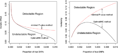
Figure 1: Left: Detection boundary on the plane of the proportion of associated SNPs and the genetic effect. Right: Detection boundary on the plane of the proportion of associated SNPs and the heritability. Solid line: the optimal boundary (reached by HC procedure); Dashed line: the boundary of the minimal $p$-value method. Here $L=10\mbox{,}000$, $n=1000$, $\sigma=1$ and $q_{j}=0.3$ for all $j$.

By equations (5) and (8)–(9), for a given proportion of true SNPs $L^{-\alpha}$, the detection boundary in (10) implies the boundaries of detectability for the genetic effects $\beta_{j}$, as well as for the genetic heritability of the trait—the proportion of total trait variation due to genetic variation:

$$\mathrm{Heritability}=\frac{\sum_{j=1}^{L}\beta_{j}^{2}2q_{j}(1-q_{j})}{\sum_{j=1}^{L}\beta_{j}^{2}2q_{j}(1-q_{j})+\sigma^{2}}.$$ (11)

For easy visualization of these boundaries, consider a special case where $|\beta_{j}|=\beta$ for $j\in M^{\ast}$ and $q_{j}=0.3$ for all $j$. The solid lines in Figure 1 illustrate the detection boundary regarding the genetic effect $\beta$ (left panel) and the detection boundary regarding the heritability (right penal) over a range of the proportion of associated SNPs corresponding to $\alpha$from $0.999$ to $0.499$.

3 Higher Criticism procedures for gene detection

The Higher Criticism (HC) procedure has been studied for the Gaussian mean model and regression model with Gaussian design matrix and known error variance [Arias-Castro, Candès and Plan (2011), Donoho and Jin (2004), Hall and Jin (2010), Ingster, Tsybakov and Verzelen (2010)]. Under the genetic model setup in (1)–(9), we adopt this procedure for gene detection based on the marginal associations between the trait and each SNP. We show that the HC procedure has asymptotically full power upon the rare and weak genetic effects exceeding the detection boundary.

Let $p_{(1)}\leq\cdots\leq p_{(L)}$ be the increasingly ordered $p$-values of $L$ individual SNPs. The HC test statistic is

$$\mathrm{HC}_{L}=\max_{1\leq j\leq L}\mathrm{HC}_{L,j}\qquad\mbox{where }\mathrm{HC}_{L,j}=\sqrt{L}\frac{(j/L)-p_{(j)}}{\sqrt{p_{(j)}(1-p_{(j)})}}.$$ (12)

In contrast to considering the minimal $p$-value in a group of SNPs, the HC considers the maximum of the normalized differences between the empirical $p$-values $j/L$ and the observed $p$-values $p_{(j)}$.

Denote the survival function of $N(0,1)$ as $\bar{\Phi}(\cdot)$. If marginal test statistics $S_{j}\sim N(0,1)$, $j=1,\ldots,L$, and the $p$-values are two-tailed, the HC statistic can be written as [Arias-Castro, Candès and Plan (2011), Donoho and Jin (2004)]

$$\mathrm{HC}_{L}=\max_{t}\mathrm{HC}_{L}(t)\qquad\mbox{where }\mathrm{HC}_{L}(t)=\frac{|\{j\dvtx|S_{j}|>t\}|-2L\bar{\Phi}(t)}{\sqrt{2L\bar{\Phi}(t)(1-2\bar{\Phi}(t))}}.$$ (13)

To study the theoretical properties of the HC procedure, for technical simplification to obtain the upper bound, we follow Arias-Castro, Candès and Plan (2011) to search for the maximum on a discrete grid and define an HC^∗ procedure with statistic

$$\mathrm{HC}^{\ast}_{L}(s)=\max\bigl{\{}\mathrm{HC}_{L}(t)\dvtx t\in{}[s,\sqrt{5\log L}]\cap\mathbb{N}\bigr{\}}.$$ (14)

In practice, we recommend to still use the straight HC in (12).

To simplify discussion, we first consider the case where $\sigma^{2}$ is known. For the genetic model in (1), let $\bar{\mathbf{Y}}=(\bar{Y},\ldots,\bar{Y})^{\prime}$ and $\bar{\mathbf{X}}_{j}=(\bar{X}_{j},\ldots,\bar{X}_{j})^{\prime}$, where $\bar{Y}=\frac{1}{n}\sum_{k=1}^{n}Y_{k}$ and $\bar{X}_{j}=\frac{1}{n}\sum_{k=1}^{n}X_{kj}$. The test statistic $S_{j}$ for the association between the trait and SNP $j$ is defined as the marginal correlation:

$$R_{j}^{\sigma}=\frac{(\mathbf{X}_{j}-\bar{\mathbf{X}}_{j})^{\prime}\mathbf{Y}}{\sigma\|\mathbf{X}_{j}-\bar{\mathbf{X}}_{j}\|},$$ (15)

where $\|\mathbf{x}\|$ is the $L^{2}$-norm of a vector $\mathbf{x}$. When SNP $j$ is not associated, we have $R_{j}^{\sigma}\rightsquigarrow N(0,1)$.

Proposition 1 states that the HC^∗ procedure reaches the optimal detection boundary. That is, for some well-controlled type I error rate converging to 0 slowly enough, the statistical power of the HC^∗ procedure converges to 1 for detecting the genetic effects that fall above the detection boundary.

Proposition 1

Consider the genetic model setup in (1)–(9). Let the marginal test statistic $S_{j}$ in (13) be $R_{j}^{\sigma}$. Under assumptions (A1), (A2.2) and (A2.4), $\mathrm{HC}^{\ast}_{L}(\sqrt{2\delta\log L})$ with $\delta=\min(1,4r^{\ast}(\alpha))$ has asymptotically full power if $r_{j}$ $>$ $r^{\ast}(\alpha)$, $j\in M^{\ast}$. Furthermore, under assumptions (A1) and (A2.5), $\mathrm{HC}^{\ast}_{L}(1)$ has asymptotically full power if $r_{j}$ $>$ $r^{\ast}(\alpha)$, $j\in M^{\ast}$.

Now we turn to a more realistic case where $\sigma$ is unknown and cannot be used in genetic association tests. We propose the following tests that incorporate $\sigma$ estimation. Specifically, the marginal association between the trait and SNP $j$ can be measured by either of the following two test statistics:

$$R_{j}=\sqrt{n-1}\rho_{j}\quad\mbox{and}\quad T_{j}=\sqrt{n-2}\rho_{j}/\sqrt{1-\rho_{j}},$$ (16)

where $\rho_{j}$ is the Pearson correlation coefficient between the observed trait values and the genotypes of the $j$th SNP. $T_{j}$ is the standard $T$-test statistic when we regress the trait on the $j$th SNP. When SNP $j$ is not associated, both $R_{j}$ and $T_{j}\rightsquigarrow N(0,1)$. Note that $R_{j}$ and $T_{j}$ are asymptotically equivalent because $\rho_{j}\rightarrow 0$ under the $\operatorname{ASW}(a,\alpha,\mathbf{r})$ model for both the null and the alternative hypotheses. The numerical results in Section 6 also show that their performances are very similar in simulations and real GWAS data analysis.

When $\sigma$ is unknown, we need a slightly stronger condition than that in Proposition 1 to guarantee the proper behavior of the $\sigma$ estimation. The following theorem shows that the HC^∗ procedure based on $R_{j}$ still reaches the detection boundary.

Theorem 2

Consider the genetic model setup in (1)–(9). Let the marginal test statistic $S_{j}$ in (13) be $R_{j}$. Under assumptions (A1), (A2.3) and (A2.4), $\mathrm{HC}^{\ast}_{L}(\sqrt{2\delta\log L})$ with $\delta=\min(1,4r^{\ast}(\alpha))$ has asymptotically full power if $r_{j}$ $>$ $r^{\ast}(\alpha)$, $j\in M^{\ast}$. Furthermore, under assumptions (A1) and (A2.5), $\mathrm{HC}^{\ast}_{L}(1)$ has asymptotically full power if $r_{j}$ $>$ $r^{\ast}(\alpha)$, $j\in M^{\ast}$.

Figure 1 illustrates that the detection boundary for the HC^∗ procedure is the same as the optimal detection boundary.

4 Connections to FDR-controlling methods

Tukey’s Higher Criticism (HC) is closely related to methods of controlling the False Discovery Rate (FDR) [e.g., Benjamini and Hochberg (1995), Efron et al. (2001)], but is also different in important ways. While there is a long line of works on FDR controlling methods, for reasons of space, we focus our discussion on Benjamini and Hochberg’s FDR-controlling method (BH), proposed in Benjamini and Hochberg (1995). The connection and difference between HC and BH can be briefly summarized as follows:

• Both BH and HC are $p$-value driven methods, the use of which needs only the $p$-values associated with all SNPs.

• BH focuses on the regime where the signals are rare but relatively strong, and the goal is signal identification.

• HC focuses on the regime where the signals are so rare and weak that signal identification is frequently impossible, but valid signal detection or screening is still possible and could be substantially helpful.

Let $p_{(1)}\leq p_{(2)}\leq\cdots\leq p_{(L)}$ be the sorted $p$-values associated with $L$ SNPs. The formulas of HC and BH are intimately connected. In detail, fix the FDR-control parameter $\alpha\in(0,1)$ (say, $\alpha=5\%$). The goal of BH is usually to control the expected fraction of false discovered SNPs out of all discovered SNPs (i.e., the FDR) so that it does not exceed $\alpha$. The procedure selects the SNPs whose $p$-values are among the $k_{\alpha}^{\mathrm{FDR}}$-smallest as discoveries, where $k_{\alpha}^{\mathrm{FDR}}$ is the largest integer $k$ such that

$$Q_{k}\leq\alpha\qquad\mbox{where }Q_{k}=\frac{p_{(k)}}{k/L}.$$

When $\min_{1\leq k\leq L}\{Q_{k}\}>\alpha$, BH reports an empty set of discoveries. $Q_{k}$ is a quantity that has been extensively studied in empirical processes. See, for example, Wellner (1978).

Following the same argument on page 975 of Donoho and Jin (2004), it can be shown that for any testing critical value $\sqrt{2q\log(L)}$ with any $0<q<1$, the ratio between the expected number of recoveries under the alternative [with signal slightly above the detection boundary in (10)] and the expected number of recoveries under the null is about 1. So the problem of BH for the rare and weak signal (which may be interesting targets in GWAS) is that

$$\min_{1\leq k\leq L}\{Q_{k}\}\approx 1.$$ (17)

As a result, for any $\alpha$ that is bounded away from $1$ (say, $\alpha\leq 90\%$), the BH method reports an empty set of discoveries. The BH method could produce a nonempty set of discoveries if we let $\alpha$ get even closer to $1$, but the FDR is so high that the set of discoveries is no longer informative for signal identification.

We will never know what was in Tukey’s mind when he proposed the Higher Criticism in 1976 [Tukey (1976)], but there is an interesting connection between HC and BH (which was proposed about 20 years later) as follows. Suppose we apply $Q_{k}$ to the HC statistic in (12). Heuristically, if $k\ll L$ and (17) holds,

$$\mathrm{HC}_{L,k}\approx\sqrt{k}(1-Q_{k}).$$

As before, think of the signal detection problem as testing a null hypothesis $H_{0}$ versus an alternative hypothesis $H_{1}^{(L)}$. In the null case where all $p$-values are i.i.d. from $U(0,1)$ and so that data contains no signal at all, then $\mathrm{HC}_{L,k}\approx N(0,1)$ for all $k$, and $\mathrm{HC}_{L,k}$ are uniformly bounded from above by a relatively small number, say, $3$. In the alternative case where the $p$-values come from rare and weak signals, even when $Q_{k}\approx 1$ for all $k$, it is still possible that for some $k$,

$$\mathrm{HC}_{L,k}\approx\sqrt{k}(1-Q_{k})\gg 1.$$

This fact says that even when signals are so rare and weak that signal identification (say, by BH) is impossible, there could still be ample space for valid inference (e.g., screening or signal detection), and HC is such a tool. Partially, we guess, this is the reason why Tukey interprets HC as the second-level significance testing.

Denote the maximizing index $k$ for $\mathrm{HC}_{L,k}$ by

$$k^{\mathrm{HC}}=\mathop{\operatorname{arg\,max}}_{1\leq k\leq L}\{\mathrm{HC}_{L,k}\}.$$

Such an index is very different from $k_{\alpha}^{\mathrm{FDR}}$. The index suggests a very interesting phenomenon that is frequently found for rare and weak signals (however, the phenomenon is not that frequently found when signals are rare and strong). Specifically, it is not always the case that $k^{\mathrm{HC}}=1$; it could happen that the index is larger than $1$, say, $k^{\mathrm{HC}}=50$. When this phenomenon happens, the interpretation is that the strongest evidence against the null is not necessarily the smallest $p$-value, but is the collection of moderately smallest $p$-values; see Donoho and Jin (2004) for discussion on moderate significances. When moderate significances contain more information for inference than does the smallest $p$-value, the HC type methodology is frequently more appropriate than BH, where the goal is shifted from signal identification to detection, to accommodate the presence of weak signals.

5 Some other gene detection procedures

With the genetic detection boundary we can show that many well-known SNP-set methods are not optimal for the rare and weak genetic effects. First, we consider the minimal $p$-value method that treats the smallest $p$-value in a SNP-set as the measurement for the association between the trait and the SNPs in the set. The following proposition considers the minimal $p$-value method under cases where $\sigma$ is either known or unknown.

Proposition 2

Consider the genetic model setup in (1)–(9). Under the assumptions (A1) and (A2.2), the minimal $p$-value procedure based on $R_{j}^{\sigma}$ has asymptotically full power if $r_{j}$ $>$ $r^{\mathrm{MP}}(\alpha)$, $j\in M^{\ast}$, and is asymptotically powerless if $r_{j}$ $<r^{\mathrm{MP}}(\alpha)$, $j\in M^{\ast}$, where

$$r^{\mathrm{MP}}(\alpha)\equiv(1-\sqrt{1-\alpha})^{2},\qquad\alpha\in(1/2,1).$$

Furthermore, under assumptions (A1) and (A2.3), the minimal $p$-value procedure based on $R_{j}$ has asymptotically full power if $r_{j}$ $>$ $r^{\mathrm{MP}}(\alpha)$, $j\in M^{\ast}$, and is asymptotically powerless if $r_{j}$ $<r^{\mathrm{MP}}(\alpha)$, $j\in M^{\ast}$.

Proposition 2 shows that the minimal $p$-value method is not optimal because $r^{\mathrm{MP}}(\alpha)$ $>r^{\ast}(\alpha)$ for $\alpha\in(1/2,3/4)$. Figure 1 illustrates the comparison between the minimal $p$-value method (dashed curve) and the HC procedure (solid curve) regarding the genetic effect ($\beta_{j}=\beta$ for all $j\in M^{\ast}$) and the heritability. When the associated SNPs are extremely rare with $\alpha\in(3/4,1)$, the two methods have the same detection boundary. However, in a wide range of the proportion of associated SNPs corresponding to $\alpha\in(1/2,3/4)$, the HC procedure can detect significantly weaker genetic effects and heritability than the minimal $p$-value method does. This regime is more important in combating the detection of the undiscovered common and rare genetic variants that could number in the hundreds [Goldstein (2009), Hall, Jin and Miller (2009), Kraft and Hunter (2009), Wade (2009)].

We further consider three commonly used SNP-set methods in the GWAS literature [Luo et al. (2010)] and show that they are not as good as the minimal $p$-value method under our model setup. Let $\mathbf{S}=(S_{1},\ldots,S_{L})^{\prime}$ be a vector of marginal test statistics and $\hat{\bolds{\Sigma}}$ be the Pearson correlation coefficients among the SNP genotypes, that is, $\hat{\bolds{\Sigma}}(i,j)=\frac{(\mathbf{X}_{i}-\bar{\mathbf{X}}_{i})^{\prime}(\mathbf{X}_{j}-\bar{\mathbf{X}}_{j})}{\|\mathbf{X}_{i}-\bar{\mathbf{X}}_{i}\|\|\mathbf{X}_{j}-\bar{\mathbf{X}}_{j}\|}$. First, the linear combination test (LCT) statistic is defined as

$$T^{L}=\mathbf{e}^{\prime}\mathbf{S}/\sqrt{\mathbf{e}^{\prime}\hat{\bolds{\Sigma}}\mathbf{e}},$$ (18)

where $\mathbf{e}$ is the vector of 1s. Second, when $\hat{\bolds{\Sigma}}^{-1}$ exists, the quadratic test (QT) statistic is defined as

$$T^{Q}=\mathbf{S}^{\prime}\hat{\bolds{\Sigma}}^{-1}\mathbf{S}.$$ (19)

Third, the decorrelation test (DT) statistic is the Fisher’s combination test after the decorrelation generating independent $p$-values:

$$T^{D}=-2\sum_{j=1}^{L}\log p_{j},$$ (20)

where the $p$-values $p_{j}=2\bar{\Phi}(|W_{j}|)$ and $W_{j}$ is the $j$th element of $\mathbf{W}=\mathbf{D}^{-1}\mathbf{S}$, where $\mathbf{D}$ is a triangular matrix of Cholesky decomposition such that $\hat{\bolds{\Sigma}}=\mathbf{D}\mathbf{D}^{\prime}$. The following theorem says that LCT, QT and DT are not optimal for rare and weak effects when SNPs are independent or have a polynomially decaying correlation along the distance between the SNPs. Specifically, for the true correlation matrix among the SNPs $\bolds{\Sigma}$, we denote the operation norm as $\|\bolds{\Sigma}\|=\sup_{\{\mathbf{a}\dvtx\|\mathbf{a}\|_{2}=1\}}\|\bolds{\Sigma}\mathbf{a}\|_{2}$. $\bolds{\Sigma}$ has a polynomial off-diagnal decay if for positive constants $M$, $\lambda$ and $C$, the magnitude of the $(j,k)$th element is upper bounded by a polynomial function

$$\bigl{|}\bolds{\Sigma}(j,k)\bigr{|}\leq M\bigl{(}1+|j-k|\bigr{)}^{-\lambda}\quad\mbox{and}\quad\|\bolds{\Sigma}\|\geq C>0.$$ (21)

Theorem 3

Consider the genetic model setup in (1)–(2), (4)–(9) and (21). The three tests in (18)–(20) correspond to $\mathbf{S}=(R_{1},\ldots,R_{L})^{\prime}$, where $R_{j}$ is defined in (16). Let $\gamma^{\prime}=\sqrt{\frac{\log L}{n}}$. For any $\lambda\geq 3$, $M\geq 1$ and $\gamma^{\prime}L=o(1)$, LCT does not have asymptotically full power when $r_{j}$ $<1$, $j\in M^{\ast}$. For any $\lambda>1$ and $\gamma^{\prime}L^{d}=o(1)$ for some $d>1$, both QT and DT do not have asymptotically full power when $r_{j}<1$, $j\in M^{\ast}$.

Because the detection boundary $r^{\mathrm{MP}}(\alpha)$ of the minimal $p$-value method is always less than $1$ for each $\alpha\in(1/2,1)$, the SNP-set methods LCT, QT and DT have poorer performance than the minimal $p$-value method. In particular, this theorem indicates that Fisher’s combination test (such as DT) is not a good choice for the rare and weak genetic effects considered here.

6 Simulations and Crohn’s disease study

Simulations and real GWAS analysis are conducted to evaluate the performance of HC-type methods and other traditional and newly proposed gene-based SNP-set methods, in which SNP genotypes in genes form sets of covariates. Instead of finding individual causative SNPs, the goal of signal detection here is to test which genes may contain these causative SNPs. Although the above theoretical results focus on model (1), in order to guide practical applications, we study both quantitative and binary traits in the following analysis of three types of data sets (Table 1): both simulated genotypes and phenotypes, real genotypes and simulated phenotypes, and both real genotypes and phenotypes for Crohn’s disease study. The following summarizes the implementation of the methods to be compared:

[1.]

Higher Criticism method. The test statistic is given in (12) for each gene. For quantitative traits, the $p$-values are calculated based on either $T_{j}$ (method denoted HC) or $R_{j}$ (denoted HCm) in (16). For binary traits, we adopt a $Z$-statistic by Zuo, Zou and Zhao (2006) (denoted HC):

$$D_{j}=\sqrt{n}\frac{\hat{p}_{\mathrm{case}}-\hat{p}_{\mathrm{control}}}{\sqrt{2\hat{p}_{\mathrm{all}}(1-\hat{p}_{\mathrm{all}})}},$$ (22)

where $\hat{p}_{\mathrm{case}}$, $\hat{p}_{\mathrm{control}}$ and $\hat{p}_{\mathrm{all}}$ are the estimated MAF in cases, controls and the combined group, respectively. When the $j$th SNP is not associated, $D_{j}\rightsquigarrow N(0,1)$, the two-tailed $p$-values $p_{j}=2\bar{\Phi}(|D_{j}|)$ are applied to (12) to get the HC statistic.

Minimal $p$-value method (denoted MinP). The association of a SNP set in a gene is determined by the smallest $p$-value $p_{(1)}$. This is the most commonly used method in GWAS practice. The $p$-values are obtained either based on $T_{j}$ in (16) for quantitative traits or $D_{j}$ in (22) for binary traits.

Principal Component Analysis (PCA) [Ballard, Cho and Zhao (2010), Wang and Abbott (2008)]. To measure the significance of a gene, a $p$-value is obtained by fitting a multiple regression for quantitative traits (or a logistic regression for binary traits) by using the least principal components that count over 85% variation.

Ridge regression (denoted Ridge) [He and Wu (2011)]. SNP covariates in a gene are fitted with traits by ridge regression at the tuning parameter that minimizes the prediction error based on cross-validation (R function lm.ridge). The residual sum of squares describes the goodness of fit of the model, and thus is treated as the score for the SNP set. The same procedure is applied to both quantitative and binary traits for simplicity.

Linear combination test (LCT), quadratic test (QT) and decorrelation test (DT) [Luo et al. (2010)]. To calculate the statistics in (18)–(20), we apply $\mathbf{S}=(T_{1},\ldots,T_{L})^{\prime}$ with $T_{j}$ in (16) for quantitative traits and $\mathbf{S}=(D_{1},\ldots,D_{L})^{\prime}$ with $D_{j}$ in (22) for binary traits.

Kernel-machine test [Wu et al. (2010)]. This is a SNP-set method that applies the generalized semiparametric models [Liu, Lin and Ghosh (2007), Wu et al. (2010)] to detect the association of genes. For the additive genetic model defined in (1), the linear kernel function is recommended by the authors [Wu et al. (2010)]. So the semiparametric model is simplified to either a multiple regression model for quantitative traits (denoted KMT) or logistic regression for binary traits (denoted LKMT). The genetic association is measured by a variance-component score statistic [Zhang and Lin (2003)]. We apply the R functions implemented by the authors of this method.

Table 1: List of the data used for analysis. Genotypes are either simulated based on six Toeplitz correlation matrices (TCM) or from the true GWAS data of NIDDK–IBDGC. The number of SNPs per gene is either 100 or according to the true data. Phenotypes are either simulated based on the additive model ($\sigma^{2}=1$) or logistic regression model ($\beta_{0}=-2$) or the true Crohn’s disease status. The locations of nonzero coefficients are always random and the values are either fixed or random, where $b_{1}$ ranges from 0.088 to 0.131 and $b_{2}$ ranges from 0.1 to 0.24

Data	Genotype	Sample	SNPs/gene	LD	MAF	Phenotype	Nonzero coefficients
1	Simulation	1000	100	6 TCM	0.4	Additive	3, $b_{1}$
2	Simulation	2000	100	6 TCM	0.4	Logit	3, $b_{2}$
3	Simulation	1000	100	6 TCM	0.4	Additive	3, $+$/$-b_{1}$ equal chance
4	Simulation	1000	100	6 TCM	0.4	Additive	3, $\operatorname{Unif}[b_{1},1.2b_{1}]$
5	Simulation	1000	100	6 TCM	0.4	Additive	3, $\operatorname{Unif}[0.9b_{1},1.1b_{1}]$
6	BCHE	851 Jew	100	real	real	Additive	3, $b_{1}$
7	BCHE	851 Jew	100	real	real	Logit	3, $b_{2}$
8	EXT1	851 Jew	106	real	real	Additive	3, $b_{1}$
9	EXT1	851 Jew	106	real	real	Logit	3, $b_{2}$
10	FSHR	851 Jew	117	real	real	Additive	3, $b_{1}$
11	FSHR	851 Jew	117	real	real	Logit	3, $b_{2}$
12	15,860 genes	851 Jew	vary	real	real	Additive	$\alpha=0.8$, $r=0.9$
13	15,860 genes	1145 non-Jewish	vary	real	real	Additive	$\alpha=0.8$, $r=0.9$
14	15,860 genes	851 Jew	vary	real	real	CD status	–
15	15,860 genes	1145 non-Jewish	vary	real	real	CD status	–

6.1 Simulated genotypes and phenotypes

We simulated both genotype and phenotype data to fully control the data structure and genetic effect pattern. Data sets 1 and 2 in Table 1 were obtained in the following. First, to simulate the genotype data, it was assumed that one gene unit contains $L=100$ SNPs, whose genotypes follow HWE in (2) with MAF $q=0.4$. To demonstrate how typical LD structures may affect these methods, six Toeplitz correlation matrices (TCM) were studied: (I) Independent SNPs, that is, the correlation matrix $\bolds{\Sigma}$ is the identity matrix. (II) SNPs in the first order neighborhoods are correlated, that is, $\bolds{\Sigma}$ has 1 in the main diagonal, 0.3 (or 0.25, or 0.2) in the first off-diagonals and 0 elsewhere. (III) SNPs are correlated with the nearest two neighbors, that is, $\bolds{\Sigma}$ has 1 in the main diagonal, 0.25 in the first off-diagonal, 0.3 (or 0.2) in the second off-diagonal and 0 elsewhere. The R package mvtBinaryEP [By and Qaqish (2011), Emrich and Piedmonte (1991)] was used to generate the correlated genotype data.

Second, to simulate the phenotype data, we considered the cases of rare and weak genetic effects based on the above theoretical results. Specifically, the rarity parameter was assumed $\alpha=0.76$, so $K=L^{1-\alpha}\approx 3$ randomly picked SNPs were made causative. Quantitative traits were generated by model (1) with error variance $\sigma^{2}=1$. The sample size was $n=1000$. We examined a series of strength parameters $r_{j}=r$ in (9) from $0.4$ to $0.9$, which correspond to the genetic effects $\beta_{j}$ in (8) equals $b_{1}$ ranging from $0.088$ to $0.131$, and the heritability of trait ranging in (11) from $0.011$ to $0.024$. On the other hand, binary traits were generated by a logistic model

$$\operatorname{logit}\biggl{(}\frac{P(Y=1|\mathbf{X})}{P(Y=0|\mathbf{X})}\biggr{)}=\beta_{0}+\beta_{1}X_{1}+\beta_{2}X_{2}+\cdots+\beta_{L}X_{L}.$$ (23)

Conditional on the genotype data, many diseased ($Y=1$) and nondiseased outcomes ($Y=0$) were generated according to the genetic risk. Then the retrospective case–control data were collected by randomly sampling $1000$ cases and $1000$ controls. We considered the coefficient $\beta_{0}=-2$ and a sequence of nonzero coefficients $\beta_{j}=b_{2}$ ranging from $0.10$ to $0.24$, which correspond to the disease allele odds ratio ranging from $1.11$ to $1.27$.

The empirical power was compared based on a well-controlled empirical type I error rate. Specifically, we ran 1000 simulations, each with newly generated genotypes, and then the phenotypes according to a specific genetic model with random locations of causative SNPs. For each simulation, we also permuted the phenotype responses and calculated the test statistics for the null hypothesis of no association. Over all simulations, the 95th percentile of the null statistics was used as the cutoffs to control the type I error rate at a level 0.05. The empirical power, that is, the true positive rate of tests, is the proportion of simulations where the test statistics exceeded the corresponding cutoff. Figures 2 and 3 show the comparisons of empirical power for data sets 1 and 2, respectively. In all the setups, the HC-type methods had the highest power. The comparisons were not significantly affected by these LD structures.

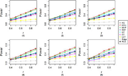
Figure 2: For quantitative traits under the fixed value of nonzero coefficients, HC and HCm have the highest power. X-axis: the strength parameter $r$ in equation (9), which corresponds to the nonzero coefficients $\beta_{j}=b_{1}$ in (8). The six panels correspond to six correlation matrices of SNPs: (1) identity matrix, (2) the 1st off-diagonals equal 0.3, (3) the 1st off-diagonals equal 0.25, (4) the 1st off-diagonals equal 0.2, (5) the 1st off-diagonals equal 0.25 and the 2nd off-diagonals equal 0.3, (6) the 1st off-diagonals equal 0.25 and the 2nd off-diagonals equal 0.2.

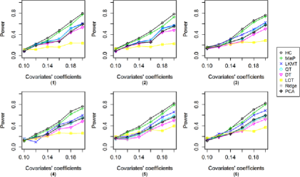
Figure 3: For binary traits from the fixed value of nonzero coefficients, HC has the highest power. X-axis: the nonzero coefficients $\beta_{j}=b_{2}$ in equation (23). The six panels correspond to the same six correlation matrices of SNPs as those in Figure 2.

In reality, causative SNPs may not have homogenous contribution to the traits. We simulated data sets 3–5 described in Table 1 for three scenarios of random genetic effects. First, the nonzero coefficients have the same magnitude $b_{1}$, but with random $+$/$-$ signs of equal probabilities. Second, the nonzero coefficients are uniformly distributed in $[b_{1},1.2b_{1}]$. Third, the nonzero coefficients are uniformly distributed in $[0.9b_{1},1.1b_{1}]$. Figure 4 shows the comparisons of the methods under random nonzero coefficients $\pm b_{1}$ with equal probabilities. HC methods were still the best among these methods assessed. Since the genetic effects have two directions, the linear combination test (LCT) causes the signals to cancel out and has low power. The results for the other two scenarios of random genetic effects (data sets 4–5 in Table 1) are given in supplementary Figures 1 and 2 [Wu et al. (2014)].

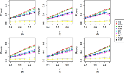
Figure 4: For quantitative traits from random nonzero coefficients $\pm b_{1}$ with equal probabilities, HC and HCm have the highest power. X-axis: the strength parameter $r$ in equation (9), which corresponds to the nonzero coefficients $\beta_{j}=b_{1}$ in (8). The six panels correspond to the same six correlation matrices of SNPs as those in Figure 2.

Our theoretical results in Sections 3–5 are about reliable detection, that is, to get asymptotically full power of detecting true genes containing a small number of weak causative SNPs. In reality, the sample size may not be large enough to allow the power approaching to 1, and there is a chance of obtaining false discoveries. Here we assessed the False Discovery Rate (FDR) of these methods over a variety of type I error rate cutoffs. Figure 5 illustrates the FDR of HC methods for quantitative traits (Data 1 in Table 1), with the strength parameter $r=0.4$–0.9. It can be seen that the FDR is well controlled, with an expected decreasing trend for increasing signal strength $r$. The HC method was also compared with other methods in terms of the FDR in supplementary Figures 3–8 [Wu et al. (2014)]. The FDR of the HC method is similar to or lower than those of the other methods.

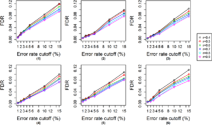
Figure 5: False Discovery Rates of the HC method for quantitative traits. X-axis: the empirical type I error rate cutoff. The six panels correspond to the same six correlation matrices of SNPs as those in Figure 2.

6.2 Real genotypes and simulated phenotypes

By using real genotype data, we studied how the real allelic distributions and LD structures, which are more complicated than the above simulations, may influence the results. For this purpose, we used the observed SNP genotypes from the data of NIDDK–IBDGC (National Institute of Diabetes, Digestive and Kidney Diseases–Inflammatory Bowel Disease Genetics Consortium) [Duerr et al. (2006)]. The data contain 851 independent subjects from the Jewish population (417 cases and 434 controls) and 1145 independent subjects from the non-Jewish population (572 cases and 573 controls). SNPs were grouped into 15,860 genes on chromosomes 1–22 according to physical locations of genes and SNPs (NCBI Human Genome Build 35). For data quality control, SNPs were excluded if they have HWE $p$-values less than 0.01 or MAF less than 0.01. SNPs were also removed if their genotypes are redundant or have a missing rate over 10%. The final data set contains 307,964 SNPs. The gene length (number of SNPs) ranges from 1 to 844 and is highly skewed to the right: the lower, median and upper quartiles are 3, 7 and 19, respectively. The missing genotypes were imputed as the average over subjects.

Quantitative and binary traits were simulated under similar setups of rare and weak genetic effects as those in Section 6.1. Data sets 6–11 in Table 1 list the parameters and setups based on three genes: BCHE (butyrylcholinesterase) is a gene with 100 SNPs located at 3q26.1-q26.2; EXT1 (exostosin 1) is a gene with 106 SNPs located at 8q24.11; FSHR (follicle stimulating hormone receptor) is a gene with 117 SNPs located at 2p21-p16. At the empirical type I error rate 0.05 from 1000 simulations, Figure 6 shows the empirical power of testing these genes through quantitative (row 1) and binary traits (row 2). It is clear that HC procedures performed similarly to or better than the other SNP-set methods.

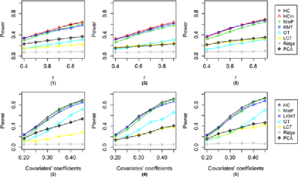
Figure 6: Power comparison based on genotype data of genes BCHE (left), EXT1 (middle) and FSHR (right), respectively. Row 1 X-axis: the strength parameter $r$ for the genetic effect in equation (9) for the quantitative trait model; row 2 X-axis: the genetic effect $\beta$ in equation (23) for the binary trait model.

We further studied the performance of these gene-detection methods when causative SNPs are simultaneously located within multiple risk genes. Specifically, we took 10 genes found to be associated with Crohn’s disease (CD) in the literature [Franke et al. (2010)] and made each of these contain $L_{g}^{1-\alpha}$ causative SNPs (rounded to integer), where $L_{g}$ is the number of SNPs in the $g$th risk gene. The locations of these associated SNPs in each risk gene were randomly chosen. The quantitative traits were then generated by an additive model (1) that contains all the causative SNPs from the 10 risk genes, where each causative SNP has a genetic effect $\beta_{j}$ defined in (8)–(9) with the rarity parameter $\alpha=0.8$ and the strength parameter $r_{j}=0.9$. After generating the quantitative trait, we carried out the GWA study by using the whole genotypes data of all 15,860 genes. Data sets 12 and 13 in Table 1 summarize the information on the parameters and setups.

To accommodate the fact that genes have distinct numbers of SNPs and LD structures, we again adapted the permutation test by randomly shuffling the response traits for obtaining the gene-by-gene empirical $p$-values. For the 10 risk genes, Tables 2 and 3 show their empirical $p$-values from $10\mbox{,}000$ permutations as well as the corresponding ranks (ties are averaged) among all 15,860 genes based on Jewish and non-Jewish data, respectively. Only HC methods reliably had the smallest average $p$-values and ranks for both data sets.

== MinP LCT QT KMT HC HCm Genes SNPs/gene Rank $\bolds{p}$-value Rank $\bolds{p}$-value Rank $\bolds{p}$-value Rank $\bolds{p}$-value Rank $\bolds{p}$-value Rank $\bolds{p}$-value IL23R $23$ $490$ $0.0314$ $1772$ $0.1138$ $2337.5$ 0.1577 $23$ $0.0007$ $109.5$ $0.0071$ $104.5$ $0.0069$ PTGER4 $72$ $3984.5$ $0.2496$ $14\mbox{,}246$ $0.901$ $2885$ 0.1931 $490$ $0.0309$ $470.5$ $0.0313$ $455$ $0.0298$ IL12B $41$ $2.5$ $0$ $15\mbox{,}574.5$ $0.9831$ $11.5$ 0.0006 $3$ $0$ $2.5$ $0$ $2.5$ $0$ CDKAL1 $160$ $2245.5$ $0.1423$ $4481$ $0.2859$ $6418.5$ 0.4155 $150$ $0.0084$ $534.5$ $0.0352$ $506.5$ $0.0335$ PRDM1 $71$ $4801.5$ $0.3029$ $2908$ $0.1858$ $5735.5$ 0.3733 $8203$ $0.5243$ $8290$ $0.5243$ $8327$ $0.5275$ ZNF365 $54$ $2.5$ $0$ $1809.5$ $0.1159$ $22$ 0.0013 $8$ $0.0002$ $2.5$ $0$ $2.5$ $0$ PLCL1 $64$ $1708.5$ $0.1092$ $8957$ $0.564$ $7353.5$ 0.4751 $338$ $0.0194$ $807.5$ $0.0505$ $768.5$ $0.049$ BACH2 $83$ $2.5$ $0$ $9747.5$ $0.6118$ $384$ 0.0274 $3$ $0$ $2.5$ $0$ $2.5$ $0$ GALC $120$ $919$ $0.0578$ $15\mbox{,}391$ $0.972$ $7146.5$ 0.4612 $1392$ $0.0948$ $936$ $0.0589$ $924.5$ $0.0581$ SMAD3 $52$ $5806.5$ $0.3642$ $4193$ $0.268$ $3079$ 0.2041 $5456$ $0.359$ $4985.5$ $0.3135$ $5024$ $0.316$ Average $74$ $1996.3$ $0.1257$ $7907.95$ $0.5001$ $3537.3$ 0.2309 .1606.6 0.1038 1614.1 0.1021 1611.9 0.1021

Table 2: Based on the NIDDK–IBDGC Jewish genotype data and the additive genetic model that contains 10 risk genes for Crohn’s disease, all 15,860 genes were tested by gene-based SNP-set method, and were ranked based on their empirical $p$-values. The ranks and $p$-values of the 10 risk genes for each method are listed, and their averages are shown in the last row

== MinP LCT QT KMT HC HCm Genes SNPs/gene Rank $\bolds{p}$-value Rank $\bolds{p}$-value Rank $\bolds{p}$-value Rank $\bolds{p}$-value Rank $\bolds{p}$-value Rank $\bolds{p}$-value IL23R $23$ $7184$ $0.4638$ $13\mbox{,}952.5$ $0.8833$ $3800.5$ 0.2603 $4979$ $0.3379$ $5626$ $0.3584$ $5635$ $0.3587$ PTGER4 $72$ $4627.5$ $0.2965$ $3859$ $0.2509$ $2983$ 0.2048 $2080$ $0.1396$ $2327.5$ $0.1449$ $2318.5$ $0.1446$ IL12B $41$ $35$ $0.0016$ $48$ $0.0026$ $2552.5$ 0.1751 $167$ $0.0075$ $29$ $0.0014$ $29.5$ $0.0013$ CDKAL1 $160$ $3$ $0.0001$ $393$ $0.0246$ $3.5$ 0.0001 $38$ $0.0011$ $4.5$ $0.0002$ $5.5$ $0.0002$ PRDM1 $71$ $878$ $0.0529$ $9258.5$ $0.5888$ $8300.5$ 0.5427 $41$ $0.0012$ $543$ $0.0322$ $517.5$ $0.0304$ ZNF365 $54$ $6080.5$ $0.3912$ $4873$ $0.313$ $4021$ 0.2741 $7593$ $0.4941$ $6857$ $0.4398$ $6837$ $0.4379$ PLCL1 $64$ $1071$ $0.0656$ $404.5$ $0.0253$ $9475$ 0.6181 $1048$ $0.0665$ $768$ $0.0479$ $777$ $0.048$ BACH2 $83$ $2357.5$ $0.1469$ $11\mbox{,}721.5$ $0.7461$ $1055.5$ 0.069 $2382$ $0.1591$ $1711$ $0.1065$ $1648.5$ $0.1032$ GALC $120$ $379.5$ $0.0232$ $14\mbox{,}902$ $0.9419$ $299.5$ 0.0209 $45$ $0.0014$ $57.5$ $0.0033$ $58.5$ $0.0033$ SMAD3 $52$ $119$ $0.0069$ $13\mbox{,}274.5$ $0.8428$ $952$ 0.0632 $2378$ $0.1588$ $98$ $0.0052$ $96$ $0.0051$ Average $74$ $2273.5$ $0.1449$ $7268.7$ $0.4619$ $3344.3$ 0.2228 $2075.1$ $0.1367$ 1802.2 0.1140 1792.3 0.1133

Table 3: Same analysis as that for Table 2, except by using the NIDDK–IBDGC non-Jewish genotype data

6.3 Real GWAS of Crohn’s disease

Crohn’s disease primarily causes ulcerations of the small and large intestines, which affects between 400,000 and 600,000 people in North America alone [Baumgart and Sandborn (2007), Loftus, Schoenfeld and Sandborn (2002)]. To detect novel risk genes of Crohn’s disease, we applied the above gene-based SNP-set methods to the NIDDK–IBDGC data that contain both real genotypes and Crohn’s disease status as the phenotype (see data sets 14 and 15 in Table 1).

The genetic architecture of Crohn’s disease remains unclear. One way to partially compare the above methods for detecting remaining risk genes is to base on risk genes that have similar properties as those undiscovered ones. In particular, we studied a set of 41 recently reported putative genes that likely contain such SNPs with rare and weak genetic effects to the susceptibility of Crohn’s disease [Table 2 of Franke et al. (2010)]. The empirical $p$-values and the corresponding ranks for these 41 genes are summarized in supplementary Tables 1 and 2 in the supplementary materials [Wu et al. (2014)] for the Jewish data and the non-Jewish data, respectively. For both data sets the HC method provided higher average ranks for the 41 risk genes than the other methods.

For the top 96 ranked genes by HC and those by MinP methods, 87 of them are common. Nine genes were included in the top 96 genes by HC, but not by MinP: PFAAP5, AGTR1, CDA08, NXPH1, LCN10, OR51G1, FDXR, KIAA1904, and EDG1. Interestingly, by the Catalogue of Somatic Mutations in Cancer (COSMIC), all nine genes contain one or more genetic variations associated to the tumor site on the large intestine. Some of these genes are likely to be relevant according to their functions. For example, PFAAP5 (human phosphonoformate immuno-associated protein 5) on chr13 is likely related to Crohn’s disease, a disease of the immune system. AGTR1 (Angiotensin II receptor type 1) on chr3 involves positive regulation of inflammatory response [The UniProt Consortium (2012)] and is associated with the increase of immunoglobulin [Wallukat et al. (1999)]. As a critical antibody in mucosal immunity, 3–5 grams of immunoglobulin is secreted daily into the intestinal lumen [Brandtzaeg and Pabst (2004)]. For NXPH1 (neurexophilin 1) on chr7, neurexophilins are signaling molecules that resemble neuropeptides by binding to alpha-neurexins and possibly other receptors. This gene may be relevant because Crohn’s disease can also present with neurological complications. Gene LCN10 is potentially relevant because biopsies of the affected colon of Crohn’s patients may show mucosal inflammation, characterized by focal infiltration of neutrophils, a type of inflammatory cell, into the epithelium [Baumgart and Sandborn (2012)]. Gene EDG1 (endothelial differentiation gene 1) has regulatory functions in normal physiology and disease processes, particularly involving the immune, and influences the delivery of systemic antigens [Arnon et al. (2011)]. Furthermore, genes AGTR1, CDA08, OR51G1 and EDG1 correspond to the components integral to membranes [Binns et al. (2009)], thus are also linked to Crohn’s disease, which is categorized as a membrane transport protein disorder. Certainly, further biological validations are needed to confirm how these genes are related to Crohn’s disease.

7 Discussion

This paper makes several contributions to the literature. First, it considers the detection boundary for rare and weak genetic effects in the GWAS setting. Second, our approach allows for marker dependencies (LD) and unknown error variance, which are lacking in theoretical consideration in the literature and are better aligned with practical GWAS settings. Third, it shows that some of the commonly used SNP-set methods are suboptimal. Fourth, it proposes a HC-based method to evaluate the statistical evidence of association between a set of SNPs and a complex trait. We show that this method achieves the most power for the specified rare and weak genetic effect setting. Application of this method to the second wave of GWAS will likely help researchers identify more trait-associated genes.

Because the values of $R$- or $T$-test statistics in (16) depend on the correlations among the genotypic covariates, the HC procedure for optimal gene detection implicitly incorporates the LD information into the hypotheses testing. For example, those SNPs correlated with an associated SNP likely have larger magnitude of their $R$- or $T$-test statistics and thus smaller marginal $p$-values. So the maximization procedure in (12) can capture this information to strengthen the genetic signal. At least in the polynomially decaying correlations defined in (21), this implicit LD-incorporation is asymptotically more powerful than some commonly applied procedures that explicitly calculate and incorporate the correlation matrix into constructing test statistics [Luo et al. (2010)], as is illustrated by Theorem 3.

This paper sheds some light on the power of genetic association studies based on marginal association tests versus joint association tests [Genovese, Jin and Wasserman (2009)]. One interesting discovery of this paper is that the HC procedure based on marginal association tests has actually reached the optimal detection boundary for the additive genetic model in (1). That is, the merit of joint association analysis is probably not for the additively joint genetic effects, but rather for gene–gene interactions [Wu and Zhao (2009, 2012)].

Although we have derived some theoretical results in this paper, and the general setup may be a reasonable abstraction of the real model, the assumptions considered are still relatively simple and may not capture the complexity of the real genetic architecture. For example, we did not consider potential gene–gene interactions that are believed to play an important role in biological systems. However, our work does represent advances over the simpler setup in the literature [Arias-Castro, Candès and Plan (2011), Donoho and Jin (2004)], with the allowance of genotype covariates and unknown environmental variance. Our theoretical results offer insights on the relative performance of different methods, which were supported by results from simulation and practical GWAS.

Our current work can lead to several future research topics in statistical genetics. The empirical null distribution may depart from $N(0,1)$ in large scale data due to unobserved covariates and/or correlations [Efron (2004, 2007a, 2007b)]. It is important to address how likely this problem could arise in gene-based detection in GWAS, and how to theoretically and practically address the issue in detecting sparse heterogeneous mixtures. From a genetics perspective, first, it would be interesting to study more complex genetic models, such as those measuring gene–gene interactions. Second, the proposed HC procedure can be extended to broader applications in genetic studies. We have illustrated the methods for gene detection based on SNP-sets grouped within genes. Depending on the scientific interests, SNPs can also be grouped based on other genomic segments or based on pathways containing sets of relevant genes [Luo et al. (2010), Yu et al. (2009)]. For example, in a pathway analysis, we can directly calculate the HC statistics using all individual SNPs within the pathway. We can also construct a two-level study, in which we calculate $p$-values for genes, for example, by the goodness-of-fit test [Donoho and Jin (2004), Section 1.6] for all SNPs within those genes, then use $p$-values of genes to calculate an HC type statistic for each pathway. These strategies will be investigated in further research.

References

- Ansorge (2009) {barticle}[pbm] \bauthor\bsnmAnsorge, \bfnmWilhelm J.\binitsW. J. (\byear2009). \btitleNext-generation DNA sequencing techniques. \bjournalN. Biotechnol. \bvolume25 \bpages195–203. \biddoi=10.1016/j.nbt.2008.12.009, issn=1871-6784, pii=S1871-6784(09)00008-9, pmid=19429539 \bptokimsref\endbibitem
- Arias-Castro, Candès and Plan (2011) {barticle}[mr] \bauthor\bsnmArias-Castro, \bfnmEry\binitsE., \bauthor\bsnmCandès, \bfnmEmmanuel J.\binitsE. J. and \bauthor\bsnmPlan, \bfnmYaniv\binitsY. (\byear2011). \btitleGlobal testing under sparse alternatives: ANOVA, multiple comparisons and the Higher Criticism. \bjournalAnn. Statist. \bvolume39 \bpages2533–2556. \biddoi=10.1214/11-AOS910, issn=0090-5364, mr=2906877 \bptokimsref\endbibitem
- Arnon et al. (2011) {barticle}[author] \bauthor\bsnmArnon, \bfnmT. I.\binitsT. I., \bauthor\bsnmXu, \bfnmY.\binitsY., \bauthor\bsnmLo, \bfnmC.\binitsC., \bauthor\bsnmPham, \bfnmT.\binitsT., \bauthor\bsnmAn, \bfnmJ.\binitsJ., \bauthor\bsnmCoughlin, \bfnmS.\binitsS., \bauthor\bsnmDorn, \bfnmG. W.\binitsG. W. and \bauthor\bsnmCyster, \bfnmJ. G.\binitsJ. G. (\byear2011). \btitleGRK2-dependent S1PR1 desensitization is required for lymphocytes to overcome their attraction to blood. \bjournalScience Signalling \bvolume333 \bpages1898. \bptokimsref\endbibitem
- Ayers and Cordell (2010) {barticle}[pbm] \bauthor\bsnmAyers, \bfnmKristin L.\binitsK. L. and \bauthor\bsnmCordell, \bfnmHeather J.\binitsH. J. (\byear2010). \btitleSNP selection in genome-wide and candidate gene studies via penalized logistic regression. \bjournalGenet. Epidemiol. \bvolume34 \bpages879–891. \biddoi=10.1002/gepi.20543, issn=1098-2272, pmcid=3410531, pmid=21104890 \bptokimsref\endbibitem
- Ballard, Cho and Zhao (2010) {barticle}[pbm] \bauthor\bsnmBallard, \bfnmDavid H.\binitsD. H., \bauthor\bsnmCho, \bfnmJudy\binitsJ. and \bauthor\bsnmZhao, \bfnmHongyu\binitsH. (\byear2010). \btitleComparisons of multi-marker association methods to detect association between a candidate region and disease. \bjournalGenet. Epidemiol. \bvolume34 \bpages201–212. \biddoi=10.1002/gepi.20448, issn=1098-2272, mid=NIHMS172277, pmcid=3158797, pmid=19810024 \bptokimsref\endbibitem
- Baumgart and Sandborn (2007) {barticle}[pbm] \bauthor\bsnmBaumgart, \bfnmDaniel C.\binitsD. C. and \bauthor\bsnmSandborn, \bfnmWilliam J.\binitsW. J. (\byear2007). \btitleInflammatory bowel disease: Clinical aspects and established and evolving therapies. \bjournalLancet \bvolume369 \bpages1641–1657. \biddoi=10.1016/S0140-6736(07)60751-X, issn=1474-547X, pii=S0140-6736(07)60751-X, pmid=17499606 \bptokimsref\endbibitem
- Baumgart and Sandborn (2012) {barticle}[author] \bauthor\bsnmBaumgart, \bfnmDaniel C.\binitsD. C. and \bauthor\bsnmSandborn, \bfnmWilliam J.\binitsW. J. (\byear2012). \btitleCrohn’s disease. \bjournalLancet \bvolume380 \bpages1590–1605. \bptokimsref\endbibitem
- Benjamini and Hochberg (1995) {barticle}[mr] \bauthor\bsnmBenjamini, \bfnmYoav\binitsY. and \bauthor\bsnmHochberg, \bfnmYosef\binitsY. (\byear1995). \btitleControlling the False Discovery Rate: A practical and powerful approach to multiple testing. \bjournalJ. R. Stat. Soc. Ser. B Stat. Methodol. \bvolume57 \bpages289–300. \bidissn=0035-9246, mr=1325392 \bptokimsref\endbibitem
- Binns et al. (2009) {barticle}[pbm] \bauthor\bsnmBinns, \bfnmDavid\binitsD., \bauthor\bsnmDimmer, \bfnmEmily\binitsE., \bauthor\bsnmHuntley, \bfnmRachael\binitsR., \bauthor\bsnmBarrell, \bfnmDaniel\binitsD., \bauthor\bsnmO’Donovan, \bfnmClaire\binitsC. and \bauthor\bsnmApweiler, \bfnmRolf\binitsR. (\byear2009). \btitleQuickGO: A web-based tool for Gene Ontology searching. \bjournalBioinformatics \bvolume25 \bpages3045–3046. \biddoi=10.1093/bioinformatics/btp536, issn=1367-4811, pii=btp536, pmcid=2773257, pmid=19744993 \bptokimsref\endbibitem
- Brandtzaeg and Pabst (2004) {barticle}[pbm] \bauthor\bsnmBrandtzaeg, \bfnmPer\binitsP. and \bauthor\bsnmPabst, \bfnmReinhard\binitsR. (\byear2004). \btitleLet’s go mucosal: Communication on slippery ground. \bjournalTrends Immunol. \bvolume25 \bpages570–577. \biddoi=10.1016/j.it.2004.09.005, issn=1471-4906, pii=S1471-4906(04)00269-8, pmid=15489184 \bptokimsref\endbibitem
- By and Qaqish (2011) {bmisc}[author] \bauthor\bsnmBy, \bfnmKunthel\binitsK. and \bauthor\bsnmQaqish, \bfnmBahjat\binitsB. (\byear2011). \bhowpublishedmvtBinaryEP: Generates correlated binary data (R package). \bptokimsref\endbibitem
- Donoho and Jin (2004) {barticle}[mr] \bauthor\bsnmDonoho, \bfnmDavid\binitsD. and \bauthor\bsnmJin, \bfnmJiashun\binitsJ. (\byear2004). \btitleHigher criticism for detecting sparse heterogeneous mixtures. \bjournalAnn. Statist. \bvolume32 \bpages962–994. \biddoi=10.1214/009053604000000265, issn=0090-5364, mr=2065195 \bptokimsref\endbibitem
- Donoho and Jin (2008) {barticle}[pbm] \bauthor\bsnmDonoho, \bfnmDavid\binitsD. and \bauthor\bsnmJin, \bfnmJiashun\binitsJ. (\byear2008). \btitleHigher criticism thresholding: Optimal feature selection when useful features are rare and weak. \bjournalProc. Natl. Acad. Sci. USA \bvolume105 \bpages14790–14795. \biddoi=10.1073/pnas.0807471105, issn=1091-6490, pii=0807471105, pmcid=2553037, pmid=18815365 \bptokimsref\endbibitem
- Duerr et al. (2006) {barticle}[author] \bauthor\bsnmDuerr, \bfnmR. H.\binitsR. H., \bauthor\bsnmTaylor, \bfnmK. D.\binitsK. D., \bauthor\bsnmBrant, \bfnmS. R.\binitsS. R., \bauthor\bsnmRioux, \bfnmJ. D.\binitsJ. D., \bauthor\bsnmSilverberg, \bfnmM. S.\binitsM. S., \bauthor\bsnmDaly, \bfnmM. J.\binitsM. J., \bauthor\bsnmSteinhart, \bfnmA. H.\binitsA. H., \bauthor\bsnmAbraham, \bfnmC.\binitsC., \bauthor\bsnmRegueiro, \bfnmM.\binitsM., \bauthor\bsnmGriffiths, \bfnmA.\binitsA. \betalet al. (\byear2006). \btitleA genome-wide association study identifies IL23R as an inflammatory bowel disease gene. \bjournalScience Signalling \bvolume314 \bpages1461. \bptokimsref\endbibitem
- Efron (2004) {barticle}[mr] \bauthor\bsnmEfron, \bfnmBradley\binitsB. (\byear2004). \btitleLarge-scale simultaneous hypothesis testing: The choice of a null hypothesis. \bjournalJ. Amer. Statist. Assoc. \bvolume99 \bpages96–104. \biddoi=10.1198/016214504000000089, issn=0162-1459, mr=2054289 \bptokimsref\endbibitem
- Efron (2007a) {barticle}[mr] \bauthor\bsnmEfron, \bfnmBradley\binitsB. (\byear2007a). \btitleCorrelation and large-scale simultaneous significance testing. \bjournalJ. Amer. Statist. Assoc. \bvolume102 \bpages93–103. \biddoi=10.1198/016214506000001211, issn=0162-1459, mr=2293302 \bptokimsref\endbibitem
- Efron (2007b) {barticle}[mr] \bauthor\bsnmEfron, \bfnmBradley\binitsB. (\byear2007b). \btitleSize, power and false discovery rates. \bjournalAnn. Statist. \bvolume35 \bpages1351–1377. \biddoi=10.1214/009053606000001460, issn=0090-5364, mr=2351089 \bptokimsref\endbibitem
- Efron et al. (2001) {barticle}[mr] \bauthor\bsnmEfron, \bfnmBradley\binitsB., \bauthor\bsnmTibshirani, \bfnmRobert\binitsR., \bauthor\bsnmStorey, \bfnmJohn D.\binitsJ. D. and \bauthor\bsnmTusher, \bfnmVirginia\binitsV. (\byear2001). \btitleEmpirical Bayes analysis of a microarray experiment. \bjournalJ. Amer. Statist. Assoc. \bvolume96 \bpages1151–1160. \biddoi=10.1198/016214501753382129, issn=0162-1459, mr=1946571 \bptokimsref\endbibitem
- Emrich and Piedmonte (1991) {barticle}[author] \bauthor\bsnmEmrich, \bfnmL. J.\binitsL. J. and \bauthor\bsnmPiedmonte, \bfnmM. R.\binitsM. R. (\byear1991). \btitleA method for generating high-dimensional multivariate binary variates. \bjournalAmer. Statist. \bvolume45 \bpages302–304. \bptokimsref\endbibitem
- Falconer, Mackay and Frankham (1996) {barticle}[author] \bauthor\bsnmFalconer, \bfnmD. S.\binitsD. S., \bauthor\bsnmMackay, \bfnmT. F. C.\binitsT. F. C. and \bauthor\bsnmFrankham, \bfnmR.\binitsR. (\byear1996). \btitleIntroduction to quantitative genetics (4th edition). \bjournalTrends in Genetics \bvolume12 \bpages280. \bptokimsref\endbibitem
- Franke et al. (2010) {barticle}[author] \bauthor\bsnmFranke, \bfnmA.\binitsA., \bauthor\bsnmMcGovern, \bfnmD. P. B.\binitsD. P. B., \bauthor\bsnmBarrett, \bfnmJ. C.\binitsJ. C., \bauthor\bsnmWang, \bfnmK.\binitsK., \bauthor\bsnmRadford-Smith, \bfnmG. L.\binitsG. L., \bauthor\bsnmAhmad, \bfnmT.\binitsT., \bauthor\bsnmLees, \bfnmC. W.\binitsC. W., \bauthor\bsnmBalschun, \bfnmT.\binitsT., \bauthor\bsnmLee, \bfnmJ.\binitsJ., \bauthor\bsnmRoberts, \bfnmR.\binitsR. \betalet al. (\byear2010). \btitleGenome-wide meta-analysis increases to 71 the number of confirmed Crohn’s disease susceptibility loci. \bjournalNature Genetics \bvolume42 \bpages1118–1125. \bptokimsref\endbibitem
- Genovese, Jin and Wasserman (2009) {bmisc}[author] \bauthor\bsnmGenovese, \bfnmC.\binitsC., \bauthor\bsnmJin, \bfnmJ.\binitsJ. and \bauthor\bsnmWasserman, \bfnmL.\binitsL. (\byear2009). \bhowpublishedRevisiting marginal regression. Preprint. Available at \arxivurlarXiv:0911.4080v1. \bptokimsref\endbibitem
- Goldstein (2009) {barticle}[pbm] \bauthor\bsnmGoldstein, \bfnmDavid B.\binitsD. B. (\byear2009). \btitleCommon genetic variation and human traits. \bjournalN. Engl. J. Med. \bvolume360 \bpages1696–1698. \biddoi=10.1056/NEJMp0806284, issn=1533-4406, pii=NEJMp0806284, pmid=19369660 \bptokimsref\endbibitem
- Guan and Stephens (2011) {barticle}[mr] \bauthor\bsnmGuan, \bfnmYongtao\binitsY. and \bauthor\bsnmStephens, \bfnmMatthew\binitsM. (\byear2011). \btitleBayesian variable selection regression for genome-wide association studies and other large-scale problems. \bjournalAnn. Appl. Stat. \bvolume5 \bpages1780–1815. \biddoi=10.1214/11-AOAS455, issn=1932-6157, mr=2884922 \bptokimsref\endbibitem
- Hall and Jin (2008) {barticle}[mr] \bauthor\bsnmHall, \bfnmPeter\binitsP. and \bauthor\bsnmJin, \bfnmJiashun\binitsJ. (\byear2008). \btitleProperties of higher criticism under strong dependence. \bjournalAnn. Statist. \bvolume36 \bpages381–402. \biddoi=10.1214/009053607000000767, issn=0090-5364, mr=2387976 \bptokimsref\endbibitem
- Hall and Jin (2010) {barticle}[mr] \bauthor\bsnmHall, \bfnmPeter\binitsP. and \bauthor\bsnmJin, \bfnmJiashun\binitsJ. (\byear2010). \btitleInnovated higher criticism for detecting sparse signals in correlated noise. \bjournalAnn. Statist. \bvolume38 \bpages1686–1732. \biddoi=10.1214/09-AOS764, issn=0090-5364, mr=2662357 \bptokimsref\endbibitem
- Hall, Jin and Miller (2009) {bmisc}[author] \bauthor\bsnmHall, \bfnmP.\binitsP., \bauthor\bsnmJin, \bfnmJ.\binitsJ. and \bauthor\bsnmMiller, \bfnmH.\binitsH. (\byear2009). \bhowpublishedFeature selection when there are many influential features. Preprint. Available at \arxivurlarXiv:0911.4076. \bptokimsref\endbibitem
- He and Wu (2011) {barticle}[author] \bauthor\bsnmHe, \bfnmS.\binitsS. and \bauthor\bsnmWu, \bfnmZ.\binitsZ. (\byear2011). \btitleGene-based Higher Criticism methods for large-scale exonic single-nucleotide polymorphism data. \bjournalBMC Proceedings \bvolume5 \bpagesS65. \bptokimsref\endbibitem
- Hoggart et al. (2008) {barticle}[author] \bauthor\bsnmHoggart, \bfnmC. J.\binitsC. J., \bauthor\bsnmWhittaker, \bfnmJ. C.\binitsJ. C., \bauthor\bsnmIorio, \bfnmM. De\binitsM. D. and \bauthor\bsnmBalding, \bfnmD. J.\binitsD. J. (\byear2008). \btitleSimultaneous analysis of all SNPs in genome-wide and re-sequencing association studies. \bjournalPLoS Genetics \bvolume4 \bpagese1000130. \bptokimsref\endbibitem
- Hoh and Ott (2003) {barticle}[pbm] \bauthor\bsnmHoh, \bfnmJosephine\binitsJ. and \bauthor\bsnmOtt, \bfnmJurg\binitsJ. (\byear2003). \btitleMathematical multi-locus approaches to localizing complex human trait genes. \bjournalNat. Rev. Genet. \bvolume4 \bpages701–709. \biddoi=10.1038/nrg1155, issn=1471-0056, pii=nrg1155, pmid=12951571 \bptokimsref\endbibitem
- Hoh, Wille and Ott (2001) {barticle}[pbm] \bauthor\bsnmHoh, \bfnmJ.\binitsJ., \bauthor\bsnmWille, \bfnmA.\binitsA. and \bauthor\bsnmOtt, \bfnmJ.\binitsJ. (\byear2001). \btitleTrimming, weighting, and grouping SNPs in human case–control association studies. \bjournalGenome Res. \bvolume11 \bpages2115–2119. \biddoi=10.1101/gr.204001, issn=1088-9051, pmcid=311222, pmid=11731502 \bptokimsref\endbibitem
- Ingster (2002) {barticle}[mr] \bauthor\bsnmIngster, \bfnmY. I.\binitsY. I. (\byear2002). \btitleAdaptive detection of a signal of growing dimension. II. \bjournalMath. Methods Statist. \bvolume11 \bpages37–68. \bidissn=1066-5307, mr=1900973 \bptokimsref\endbibitem
- Ingster, Tsybakov and Verzelen (2010) {barticle}[mr] \bauthor\bsnmIngster, \bfnmYuri I.\binitsY. I., \bauthor\bsnmTsybakov, \bfnmAlexandre B.\binitsA. B. and \bauthor\bsnmVerzelen, \bfnmNicolas\binitsN. (\byear2010). \btitleDetection boundary in sparse regression. \bjournalElectron. J. Stat. \bvolume4 \bpages1476–1526. \biddoi=10.1214/10-EJS589, issn=1935-7524, mr=2747131 \bptokimsref\endbibitem
- Jin and Wang (2013) {bmisc}[author] \bauthor\bsnmJin, \bfnmJ.\binitsJ. and \bauthor\bsnmWang, \bfnmL.\binitsL. (\byear2013). \bhowpublishedSpectral clustering by Higher Criticism Thresholding. Unpublished manuscript. \bptokimsref\endbibitem
- Kraft and Hunter (2009) {barticle}[author] \bauthor\bsnmKraft, \bfnmP.\binitsP. and \bauthor\bsnmHunter, \bfnmD. J.\binitsD. J. (\byear2009). \btitleGenetic risk prediction—Are we there yet? \bjournalNew England Journal of Medicine \bvolume360 \bpages1701. \bptokimsref\endbibitem
- Li et al. (2009) {barticle}[pbm] \bauthor\bsnmLi, \bfnmMingyao\binitsM., \bauthor\bsnmWang, \bfnmKai\binitsK., \bauthor\bsnmGrant, \bfnmStruan F. A.\binitsS. F. A., \bauthor\bsnmHakonarson, \bfnmHakon\binitsH. and \bauthor\bsnmLi, \bfnmChun\binitsC. (\byear2009). \btitleATOM: A powerful gene-based association test by combining optimally weighted markers. \bjournalBioinformatics \bvolume25 \bpages497–503. \biddoi=10.1093/bioinformatics/btn641, issn=1367-4811, pii=btn641, pmcid=2642636, pmid=19074959 \bptokimsref\endbibitem
- Liu, Lin and Ghosh (2007) {barticle}[mr] \bauthor\bsnmLiu, \bfnmDawei\binitsD., \bauthor\bsnmLin, \bfnmXihong\binitsX. and \bauthor\bsnmGhosh, \bfnmDebashis\binitsD. (\byear2007). \btitleSemiparametric regression of multidimensional genetic pathway data: Least-squares kernel machines and linear mixed models. \bjournalBiometrics \bvolume63 \bpages1079–1088, 1311. \biddoi=10.1111/j.1541-0420.2007.00799.x, issn=0006-341X, mr=2414585 \bptokimsref\endbibitem
- Loftus, Schoenfeld and Sandborn (2002) {barticle}[author] \bauthor\bsnmLoftus, \bfnmE. V.\binitsE. V., \bauthor\bsnmSchoenfeld, \bfnmP.\binitsP. and \bauthor\bsnmSandborn, \bfnmW. J.\binitsW. J. (\byear2002). \btitleThe epidemiology and natural history of Crohn’s disease in population-based patient cohorts from North America: A systematic review. \bjournalAlimentary Pharmacology & Therapeutics \bvolume16 \bpages51–60. \bptokimsref\endbibitem
- Luo et al. (2010) {barticle}[pbm] \bauthor\bsnmLuo, \bfnmLi\binitsL., \bauthor\bsnmPeng, \bfnmGang\binitsG., \bauthor\bsnmZhu, \bfnmYun\binitsY., \bauthor\bsnmDong, \bfnmHua\binitsH., \bauthor\bsnmAmos, \bfnmChristopher I.\binitsC. I. and \bauthor\bsnmXiong, \bfnmMomiao\binitsM. (\byear2010). \btitleGenome-wide gene and pathway analysis. \bjournalEur. J. Hum. Genet. \bvolume18 \bpages1045–1053. \biddoi=10.1038/ejhg.2010.62, issn=1476-5438, mid=NIHMS187627, pii=ejhg201062, pmcid=2924916, pmid=20442747 \bptokimsref\endbibitem
- Mardis (2008) {barticle}[pbm] \bauthor\bsnmMardis, \bfnmElaine R.\binitsE. R. (\byear2008). \btitleNext-generation DNA sequencing methods. \bjournalAnnu. Rev. Genomics Hum. Genet. \bvolume9 \bpages387–402. \biddoi=10.1146/annurev.genom.9.081307.164359, issn=1527-8204, pmid=18576944 \bptokimsref\endbibitem
- McCarthy et al. (2008) {barticle}[pbm] \bauthor\bsnmMcCarthy, \bfnmMark I.\binitsM. I., \bauthor\bsnmAbecasis, \bfnmGonçalo R.\binitsG. R., \bauthor\bsnmCardon, \bfnmLon R.\binitsL. R., \bauthor\bsnmGoldstein, \bfnmDavid B.\binitsD. B., \bauthor\bsnmLittle, \bfnmJulian\binitsJ., \bauthor\bsnmIoannidis, \bfnmJohn P. A.\binitsJ. P. A. and \bauthor\bsnmHirschhorn, \bfnmJoel N.\binitsJ. N. (\byear2008). \btitleGenome-wide association studies for complex traits: Consensus, uncertainty and challenges. \bjournalNat. Rev. Genet. \bvolume9 \bpages356–369. \biddoi=10.1038/nrg2344, issn=1471-0064, pii=nrg2344, pmid=18398418 \bptokimsref\endbibitem
- Mendel (1866) {barticle}[author] \bauthor\bsnmMendel, \bfnmG.\binitsG. (\byear1866). \btitleVersuche über Pflanzen-Hybriden. Verhandlungen des naturforschenden Vereines in Brünn, Bd. IV for das Jahr 1865, Abhandlungen, 3–47. \bjournalGenetic Theory \bvolume295 \bpages3–47. \bptokimsref\endbibitem
- Metzker (2010) {barticle}[pbm] \bauthor\bsnmMetzker, \bfnmMichael L.\binitsM. L. (\byear2010). \btitleSequencing technologies—The next generation. \bjournalNat. Rev. Genet. \bvolume11 \bpages31–46. \biddoi=10.1038/nrg2626, issn=1471-0064, pii=nrg2626, pmid=19997069 \bptnotecheck year \bptokimsref\endbibitem
- Mukhopadhyay et al. (2010) {barticle}[pbm] \bauthor\bsnmMukhopadhyay, \bfnmIndranil\binitsI., \bauthor\bsnmFeingold, \bfnmEleanor\binitsE., \bauthor\bsnmWeeks, \bfnmDaniel E.\binitsD. E. and \bauthor\bsnmThalamuthu, \bfnmAnbupalam\binitsA. (\byear2010). \btitleAssociation tests using kernel-based measures of multi-locus genotype similarity between individuals. \bjournalGenet. Epidemiol. \bvolume34 \bpages213–221. \biddoi=10.1002/gepi.20451, issn=1098-2272, mid=NIHMS350293, pmcid=3272581, pmid=19697357 \bptokimsref\endbibitem
- Pearson (1904) {barticle}[author] \bauthor\bsnmPearson, \bfnmK.\binitsK. (\byear1904). \btitleMathematical contributions to the theory of evolution. XII. On a generalised theory of alternative inheritance, with special reference to Mendel’s laws. \bjournalPhilos. Trans. R. Soc. Lond. Ser. A Math. Phys. Eng. Sci. \bvolume203 \bpages53–86. \bptokimsref\endbibitem
- Peng et al. (2009) {barticle}[author] \bauthor\bsnmPeng, \bfnmG.\binitsG., \bauthor\bsnmLuo, \bfnmL.\binitsL., \bauthor\bsnmSiu, \bfnmH.\binitsH., \bauthor\bsnmZhu, \bfnmY.\binitsY., \bauthor\bsnmHu, \bfnmP.\binitsP., \bauthor\bsnmHong, \bfnmS.\binitsS., \bauthor\bsnmZhao, \bfnmJ.\binitsJ., \bauthor\bsnmZhou, \bfnmX.\binitsX., \bauthor\bsnmReveille, \bfnmJ. D.\binitsJ. D. and \bauthor\bsnmJin, \bfnmL.\binitsL. (\byear2009). \btitleGene and pathway-based second-wave analysis of genome-wide association studies. \bjournalEuropean Journal of Human Genetics \bvolume18 \bpages111–117. \bptokimsref\endbibitem
- The UniProt Consortium (2012) {bmisc}[author] \borganizationThe UniProt Consortium (\byear2012). \bhowpublishedReorganizing the protein space at the Universal Protein Resource (UniProt). Nucleic. Acids Res. 40 D71–D75. \bptokimsref\endbibitem
- Tukey (1976) {bmisc}[author] \bauthor\bsnmTukey, \bfnmJ. W.\binitsJ. W. (\byear1976). \bhowpublishedThe higher criticism. Course Notes, Statistics 411, Princeton Univ. \bptokimsref\endbibitem
- Wade (2009) {bmisc}[author] \bauthor\bsnmWade, \bfnmN.\binitsN. (\byear2009). \bhowpublishedGenes show limited value in predicting diseases. New York Times April 16. \bptokimsref\endbibitem
- Wallukat et al. (1999) {barticle}[author] \bauthor\bsnmWallukat, \bfnmG.\binitsG., \bauthor\bsnmHomuth, \bfnmV.\binitsV., \bauthor\bsnmFischer, \bfnmT.\binitsT., \bauthor\bsnmLindschau, \bfnmC.\binitsC., \bauthor\bsnmHorstkamp, \bfnmB.\binitsB., \bauthor\bsnmJüpner, \bfnmA.\binitsA., \bauthor\bsnmBaur, \bfnmE.\binitsE., \bauthor\bsnmNissen, \bfnmE.\binitsE., \bauthor\bsnmVetter, \bfnmK.\binitsK., \bauthor\bsnmNeichel, \bfnmD.\binitsD. \betalet al. (\byear1999). \btitlePatients with preeclampsia develop agonistic autoantibodies against the angiotensin AT1 receptor. \bjournalJournal of Clinical Investigation \bvolume103 \bpages945–952. \bptokimsref\endbibitem
- Wang and Abbott (2008) {barticle}[pbm] \bauthor\bsnmWang, \bfnmKai\binitsK. and \bauthor\bsnmAbbott, \bfnmDiana\binitsD. (\byear2008). \btitleA principal components regression approach to multilocus genetic association studies. \bjournalGenet. Epidemiol. \bvolume32 \bpages108–118. \biddoi=10.1002/gepi.20266, issn=0741-0395, pmid=17849491 \bptokimsref\endbibitem
- Wang, Li and Bucan (2007) {barticle}[pbm] \bauthor\bsnmWang, \bfnmKai\binitsK., \bauthor\bsnmLi, \bfnmMingyao\binitsM. and \bauthor\bsnmBucan, \bfnmMaja\binitsM. (\byear2007). \btitlePathway-based approaches for analysis of genomewide association studies. \bjournalAm. J. Hum. Genet. \bvolume81 \bpages1278–1283. \biddoi=10.1086/522374, issn=1537-6605, pii=S0002929707637756, pmcid=2276352, pmid=17966091 \bptokimsref\endbibitem
- Wellner (1978) {barticle}[mr] \bauthor\bsnmWellner, \bfnmJon A.\binitsJ. A. (\byear1978). \btitleLimit theorems for the ratio of the empirical distribution function to the true distribution function. \bjournalZ. Wahrsch. Verw. Gebiete \bvolume45 \bpages73–88. \bidissn=0178-8051, mr=0651392 \bptokimsref\endbibitem
- Wu and Zhao (2009) {barticle}[pbm] \bauthor\bsnmWu, \bfnmZheyang\binitsZ. and \bauthor\bsnmZhao, \bfnmHongyu\binitsH. (\byear2009). \btitleStatistical power of model selection strategies for genome-wide association studies. \bjournalPLoS Genet. \bvolume5 \bpagese1000582. \biddoi=10.1371/journal.pgen.1000582, issn=1553-7404, pmcid=2712761, pmid=19649321 \bptokimsref\endbibitem
- Wu and Zhao (2012) {barticle}[mr] \bauthor\bsnmWu, \bfnmZheyang\binitsZ. and \bauthor\bsnmZhao, \bfnmHongyu\binitsH. (\byear2012). \btitleOn model selection strategies to identify genes underlying binary traits using genome-wide association data. \bjournalStatist. Sinica \bvolume22 \bpages1041–1074. \biddoi=10.5705/ss.2010.183, issn=1017-0405, mr=2987483 \bptokimsref\endbibitem
- Wu et al. (2009) {barticle}[pbm] \bauthor\bsnmWu, \bfnmTong Tong\binitsT. T., \bauthor\bsnmChen, \bfnmYi Fang\binitsY. F., \bauthor\bsnmHastie, \bfnmTrevor\binitsT., \bauthor\bsnmSobel, \bfnmEric\binitsE. and \bauthor\bsnmLange, \bfnmKenneth\binitsK. (\byear2009). \btitleGenome-wide association analysis by lasso penalized logistic regression. \bjournalBioinformatics \bvolume25 \bpages714–721. \biddoi=10.1093/bioinformatics/btp041, issn=1367-4811, pii=btp041, pmcid=2732298, pmid=19176549 \bptokimsref\endbibitem
- Wu et al. (2010) {barticle}[pbm] \bauthor\bsnmWu, \bfnmMichael C.\binitsM. C., \bauthor\bsnmKraft, \bfnmPeter\binitsP., \bauthor\bsnmEpstein, \bfnmMichael P.\binitsM. P., \bauthor\bsnmTaylor, \bfnmDeanne M.\binitsD. M., \bauthor\bsnmChanock, \bfnmStephen J.\binitsS. J., \bauthor\bsnmHunter, \bfnmDavid J.\binitsD. J. and \bauthor\bsnmLin, \bfnmXihong\binitsX. (\byear2010). \btitlePowerful SNP-set analysis for case–control genome-wide association studies. \bjournalAm. J. Hum. Genet. \bvolume86 \bpages929–942. \biddoi=10.1016/j.ajhg.2010.05.002, issn=1537-6605, pii=S0002-9297(10)00248-X, pmcid=3032061, pmid=20560208 \bptokimsref\endbibitem
- Wu et al. (2014) {bmisc}[author] \bauthor\bsnmWu, \bfnmZheyang\binitsZ., \bauthor\bsnmSun, \bfnmYiming\binitsY., \bauthor\bsnmHe, \bfnmShiquan\binitsS., \bauthor\bsnmCho, \bfnmJudy H.\binitsJ. H., \bauthor\bsnmZhao, \bfnmHongyu\binitsH. and \bauthor\bsnmJin, \bfnmJiashun\binitsJ. (\byear2014). \bhowpublishedSupplement to “Detection boundary and Higher Criticism approach for rare and weak genetic effects.” DOI:\doiurl10.1214/14-AOAS724SUPP. \bptokimsref \endbibitem
- Xie, Cai and Li (2011) {barticle}[mr] \bauthor\bsnmXie, \bfnmJichun\binitsJ., \bauthor\bsnmCai, \bfnmT. Tony\binitsT. T. and \bauthor\bsnmLi, \bfnmHongzhe\binitsH. (\byear2011). \btitleSample size and power analysis for sparse signal recovery in genome-wide association studies. \bjournalBiometrika \bvolume98 \bpages273–290. \biddoi=10.1093/biomet/asr003, issn=0006-3444, mr=2806428 \bptokimsref\endbibitem
- Yang, Hsieh and Fann (2008) {barticle}[author] \bauthor\bsnmYang, \bfnmH. C.\binitsH. C., \bauthor\bsnmHsieh, \bfnmH. Y.\binitsH. Y. and \bauthor\bsnmFann, \bfnmC. S. J.\binitsC. S. J. (\byear2008). \btitleKernel-based association test. \bjournalGenetics \bvolume179 \bpages1057–1068. \bptokimsref\endbibitem
- Yu et al. (2009) {barticle}[pbm] \bauthor\bsnmYu, \bfnmKai\binitsK., \bauthor\bsnmLi, \bfnmQizhai\binitsQ., \bauthor\bsnmBergen, \bfnmAndrew W.\binitsA. W., \bauthor\bsnmPfeiffer, \bfnmRuth M.\binitsR. M., \bauthor\bsnmRosenberg, \bfnmPhilip S.\binitsP. S., \bauthor\bsnmCaporaso, \bfnmNeil\binitsN., \bauthor\bsnmKraft, \bfnmPeter\binitsP. and \bauthor\bsnmChatterjee, \bfnmNilanjan\binitsN. (\byear2009). \btitlePathway analysis by adaptive combination of -values. \bjournalGenet. Epidemiol. \bvolume33 \bpages700–709. \biddoi=10.1002/gepi.20422, issn=1098-2272, mid=NIHMS117665, pmcid=2790032, pmid=19333968 \bptokimsref\endbibitem
- Yulh (1902) {barticle}[author] \bauthor\bsnmYulh, \bfnmG. U.\binitsG. U. (\byear1902). \btitleMendel’s laws and their probable relations to intra-racial heredity. \bjournalThe New Phytologist \bvolume1 \bpages193–207. \bptokimsref\endbibitem
- Zhang and Lin (2003) {barticle}[pbm] \bauthor\bsnmZhang, \bfnmDaowen\binitsD. and \bauthor\bsnmLin, \bfnmXihong\binitsX. (\byear2003). \btitleHypothesis testing in semiparametric additive mixed models. \bjournalBiostatistics \bvolume4 \bpages57–74. \biddoi=10.1093/biostatistics/4.1.57, issn=1465-4644, pii=4/1/57, pmid=12925330 \bptokimsref\endbibitem
- Zuo, Zou and Zhao (2006) {barticle}[pbm] \bauthor\bsnmZuo, \bfnmYijun\binitsY., \bauthor\bsnmZou, \bfnmGuohua\binitsG. and \bauthor\bsnmZhao, \bfnmHongyu\binitsH. (\byear2006). \btitleTwo-stage designs in case–control association analysis. \bjournalGenetics \bvolume173 \bpages1747–1760. \biddoi=10.1534/genetics.105.042648, issn=0016-6731, pii=genetics.105.042648, pmcid=1526674, pmid=16624925 \bptokimsref\endbibitem