Small area estimation of general parameters with application to poverty indicators: A hierarchical Bayes approach

Abstract

Poverty maps are used to aid important political decisions such as allocation of development funds by governments and international organizations. Those decisions should be based on the most accurate poverty figures. However, often reliable poverty figures are not available at fine geographical levels or for particular risk population subgroups due to the sample size limitation of current national surveys. These surveys cannot cover adequately all the desired areas or population subgroups and, therefore, models relating the different areas are needed to “borrow strength” from area to area. In particular, the Spanish Survey on Income and Living Conditions (SILC) produces national poverty estimates but cannot provide poverty estimates by Spanish provinces due to the poor precision of direct estimates, which use only the province specific data. It also raises the ethical question of whether poverty is more severe for women than for men in a given province. We develop a hierarchical Bayes (HB) approach for poverty mapping in Spanish provinces by gender that overcomes the small province sample size problem of the SILC. The proposed approach has a wide scope of application because it can be used to estimate general nonlinear parameters. We use a Bayesian version of the nested error regression model in which Markov chain Monte Carlo procedures and the convergence monitoring therein are avoided. A simulation study reveals good frequentist properties of the HB approach. The resulting poverty maps indicate that poverty, both in frequency and intensity, is localized mostly in the southern and western provinces and it is more acute for women than for men in most of the provinces.

, and t1Supported in part by the Spanish Grants MTM2009-09473 and SEJ2007-64500 from the Spanish Ministerio de Educación y Ciencia. t2Supported in part by the Natural Sciences and Engineering Research Council of Canada.

1 Introduction

Before the recent world economic crisis, the goal of a 23% maximum global poverty rate established in the United Nations Millennium Development Goals for the year 2015 seemed to be easy to achieve and there was also a clear indication of progress in all the other goals. However, after the crisis and also due to the late environmental disasters such as the drought in East Africa, the situation regarding poverty is getting worse. A reliable and detailed statistical measurement is certainly essential in the assessment of the well being of different regions, which will lead to the design of effective developmental policies.

Often, national surveys are not designed to give reliable statistics at the local level. This is the case of the Spanish Survey on Income and Living Conditions (SILC), which is planned to produce estimates for poverty incidence at the Spanish Autonomous Communities (large regions), but it cannot provide estimates for Spanish provinces due to the small SILC sample sizes for some of the provinces. The population subdivisions, not necessarily geographical, which constitute the estimation domains, will be called in general “areas.” When estimating some aggregate characteristic of an area, a “direct” estimator is the one that uses solely the data from that area. These estimators are often design unbiased, at least approximately. However, they have overly large sampling errors for areas with small sample sizes. The areas with inadequate sample sizes are labeled as “small areas.” This problem has given rise to the development of the scientific field called small area estimation, which studies “indirect” estimation methods that “borrow strength” from related areas. Some of these methods are based on explicit models that link all areas through common parameters and making use of auxiliary information. Such model-based techniques are appealing because they provide estimators with high efficiency even under very small area-specific sample sizes. The monograph of Rao (2003) contains a comprehensive account of small area estimation techniques that appeared until the publication date; see Jiang and Lahiri (2006), Datta (2009) and Pfeffermann (2013) for reviews of the more recent work.

Small area models may be classified into two broad types: (i) Area-level models that relate small area direct estimates to area-specific covariates, and (ii) Unit-level models that relate the unit values of a study variable to associated unit-specific covariates and possibly also area-specific covariates. So far, most of the model-based small area methods have focused on the estimation of totals and means, and nonlinear parameters have not received much attention. However, many poverty and inequality indicators are rather complex nonlinear functions of the income or other welfare measures of individuals; see, for example, Neri, Ballini and Betti (2005). The main purpose of this paper is to develop a suitable method, based on the hierarchical Bayes approach, to handle general nonlinear parameters. We, however, focus on poverty indicators as particular cases due to the important socio-economic impact of this application.

Hierarchical Bayesian models have been extensively used in small area estimation; see Rao (2003), Chapter 10 and Datta (2009). A hierarchical Bayesian model can accommodate very complex models for the data based on very simple models as building blocks. For example, within the Bayesian paradigm, by making parameters stochastic, one can introduce an intracluster correlation and different sources of variability can be also incorporated. In small area estimation, the hierarchical Bayesian model provides the much needed “borrowing of strength” in a simple manner; see, for example, Nandram and Choi (2005, 2010), where hierarchical Bayesian models are used to study body mass index on the continuous scale. You and Zhou (2011) use a spatial hierarchical Bayes model in an application to health survey data. Finally, Mohadjer et al. (2012) study small area estimation of adult literacy in the U.S. using unmatched sampling and linking models, using hierarchical Bayes methods.

In the context of poverty estimation, area-level models have been used to estimate the proportion of school age children under poverty at the county level under the SAIPE program (Small Area Income and Poverty Estimates) of the U.S. Census Bureau; for more details, see, for example, Bell (1997) or the program webpage http://www.census.gov/did/www/saipe/. Using the Spanish SILC data, Molina and Morales (2009) used an area-level model relating direct estimates of poverty proportions and poverty gaps (defined in Section 2) to area covariates obtained from a much larger survey, the Labor Force Survey (LFS). In this application, the areas are the Spanish provinces. Results based on the empirical best (or Bayes) approach for this area-level model indicated only marginal gains in efficiency over direct estimates.

Few approaches have appeared in the literature for efficient estimation of general nonlinear indicators using unit-level models. Here we discuss the most popular ones. The first one, due to Elbers, Lanjouw and Lanjouw (2003), is the method used by the World Bank (WB). This method was designed specially to deal with complex nonlinear poverty indicators. It assumes that the log incomes of the individuals in the population follow a unit-level model similar to the nested error linear regression model of Battese, Harter and Fuller (1988), but including random effects for sampling clusters instead of area effects. After fitting the model to survey data, the WB method generates by bootstrap resampling a number of synthetic censuses making use of census auxiliary data and the fitted model. From each synthetic census, a poverty indicator of interest is computed for each small area. The average of the estimates over simulated censuses is then taken as the point estimate of the poverty indicator, and the variance of the estimates is taken as a measure of variability. The WB used the above simple method to produce poverty maps for many countries, by securing census auxiliary data and income data from a sample survey. In European countries, registers that provide unit-level population data may be obtained through collaboration with statistical offices. In Scandinavian countries and in Switzerland, continuously updated census auxiliary unit-level data are available through statistical offices. We emphasize that unit level auxiliary data for the population is needed to implement the WB method, based on a unit-level model, to estimate small area poverty indicators or other complex parameters; area means of the auxiliary variables would be sufficient in the case of estimating area means of a variable of interest.

The second approach for estimation of general small area parameters, based on the empirical best/Bayes (EB) method, was recently introduced by Molina and Rao (2010). This method gives estimators with minimum mean squared error called best predictors or, more exactly, Monte Carlo approximations to the best predictors. This is done under the assumption that there exists a transformation of the incomes of individuals or another welfare variable used to measure poverty such that the transformed incomes follow the nested error regression model of Battese, Harter and Fuller (1988). Mean squared errors of the EB estimators are estimated by a parametric bootstrap method. The method of Molina and Rao (2010) also requires unit-level auxiliary data for the population.

Both methods approximate an expected value by Monte Carlo, which requires generation of many full synthetic censuses that might be of huge size (e.g., over 43 million in the Spanish application of Section 5). In addition, the mean squared error is estimated using the bootstrap (or double bootstrap) in which the expected values need to be approximated for each bootstrap (or double bootstrap) replicate. The full procedure might be very intensive computationally and even may not be feasible for very complex poverty indicators such as those requiring sorting population elements or for very large populations such as Brazil or India.

The hierarchical Bayes method is a good alternative to EB because it does not require the use of bootstrap for mean squared error estimation and it provides credible intervals and other useful summaries from the posterior distributions with practically no additional effort. We propose a very simple hierarchical Bayes (HB) approach that is computationally much more efficient than the alternative EB procedure. Only noninformative priors are considered to save us from the introduction of subjective information which might be controversial in official statistics applications. Moreover, using a particular reparameterization of the model and noninformative priors, we avoid the use of Markov chain Monte Carlo (MCMC) methods and therefore also the need for monitoring convergence of the Markov chains for each generated sample in the simulation studies, but ensuring propriety of the posterior under general conditions. In our simulations, this HB method provides point estimates that are practically the same as EB estimates and inferences that have frequentist validity. This frequentist validity gives a strong support to the use of the proposed HB method in practice.

2 Poverty indicators

Certainly, poverty and income inequality are broad and complex concepts which cannot be easily summarized in one measure or indicator. In the literature there are many different indicators intending to summarize poverty or income inequality in one measure, each of them focusing on the measurement of particular aspects of poverty. For a summary of poverty and inequality indicators see, for example, Neri, Ballini and Betti (2005). Basic poverty indicators are the head count ratio, referred to here as poverty incidence, which is simply the proportion of individuals with welfare measure under the poverty line, and the poverty gap, measuring the mean relative distance to the poverty line of the individuals with welfare measure under the poverty line. The class of poverty indicators introduced by Foster, Greer and Thorbecke (1984) contains the previous two as particular cases. Other measures include the Sen Index, the Fuzzy monetary and the Fuzzy supplementary poverty indicators [Betti et al. (2006)]. Practically all poverty measures are rather complex nonlinear functions of the income or some other welfare measure of individuals. We will introduce HB methodology that is suitable for the estimation of general nonlinear parameters, but we illustrate the procedure by applying it to particular indicators of interest, namely, the poverty incidence and the poverty gap as in Molina and Rao (2010). This will allow comparison with the EB method introduced in that paper.

Let us consider a population of size $N$ that is partitioned into $D$ subpopulations of sizes $N_{1},\ldots,N_{D}$ and called small areas. Let $E_{di}$ be a suitable quantitative measure of welfare for individual $i$ in small area $d$, such as income or expenditure, and let $z$ be the poverty line, that is, the threshold for $E_{di}$ under which a person is considered as “under poverty.” The family of poverty measures of Foster, Greer and Thorbecke (1984) for a small area $d$ may be expressed as

$$F_{\alpha d}=\frac{1}{N_{d}}\sum_{i=1}^{N_{d}}\biggl{(}\frac{z-E_{di}}{z}\biggr{)}^{\alpha}I(E_{di}<z),\qquad\alpha\geq 0,d=1,\ldots,D,$$

where $I(E_{di}<z)=1$ if $E_{di}<z$ or the person is under poverty and$I(E_{di}<z)=0$ if $E_{di}\geq z$ or the person is not under poverty. Taking $\alpha=0$, we obtain the area poverty incidence, which measures the frequency of the poverty, and $\alpha=1$ leads to the area poverty gap, which quantifies the intensity of the poverty.

3 Hierarchical Bayes predictors of poverty indicators

Estimation of the target area characteristics is based on a random sample drawn from the finite population according to a specified sampling design. Let $P$ denote the set of indices of the population units, $s$ be the set of units selected in the sample, of size $n<N$, and $r=P-s$ be the set of the units, with size $N-n$, that are not selected. Let $P_{d}$, $s_{d}$, $r_{d}$, $N_{d}$ and $n_{d}$ be, respectively, the set of population units, sample, sample complement, population size and sample size, restricted to area $d$. We allow zero sample sizes for some of the areas. Without loss of generality, we assume that those areas are the last $D-D^{*}$ areas, that is, $n_{d}>0$, for $d=1,\ldots,D^{*}$, where $D^{*}\leq D$, and $n_{d}=0$ for $d=D^{*}+1,\ldots,D$. Then the overall sample size is $n=n_{1}+\cdots+n_{D^{*}}$. For $d=D^{*}+1,\ldots,D$ with $n_{d}=0$, we have $s_{d}=\varnothing$ and $r_{d}=P_{d}$.

To estimate $F_{\alpha d}$ efficiently for each area $d$, we assume that there are $p$ auxiliary variables related linearly to some one-to-one transformation $Y_{di}=T(E_{di})$ of the welfare variables. More concretely, we assume that the transformed population values $\{Y_{di};i=1,\ldots,N_{d}\}$ follow the nested error model

$$Y_{di}=\mathbf{x}_{di}^{\prime}\bolds{\beta}+u_{d}+e_{di},\qquad i=1,\ldots,N_{d},d=1,\ldots,D,$$ (1)

introduced by Battese, Harter and Fuller (1988), where $\mathbf{x}_{di}$ is the $p\times 1$ vector of auxiliary variables for unit $i$ within area $d$, $\bolds{\beta}$ is the $p\times 1$ (constant) vector of regression coefficients associated with $\mathbf{x}_{di}$, $u_{d}$ is a random effect of area $d$, which models the unexplained between area variation, and $e_{di}$ is the individual model error. Area effects $u_{d}$ and errors $e_{di}$ given all parameters are independent and satisfy, respectively, $u_{d}|\sigma_{u}^{2}\stackrel{{\scriptstyle\mathrm{i.i.d.}}}{{\sim}}N(0,\sigma_{u}^{2})$ and $e_{di}|\sigma^{2}\stackrel{{\scriptstyle\mathrm{i.i.d.}}}{{\sim}}N(0,\sigma^{2}w_{di}^{-1})$, where $w_{di}>0$ is a known heteroscedasticity weight. In practice, these weights can be obtained from a preliminary modeling of error variances using variables different from those considered in the mean model as done in the WB method. We assume that the values of the auxiliary variables are known for all population units.

MCMC is a popular tool used to implement the HB method and software such as WinBUGS is readily available. However, running the Gibbs sampler requires monitoring the convergence by making a long run, thinning and performing convergence tests. In simulation studies, this monitoring process must be done for each simulated data set. Failing to do this carefully might lead to gross approximation of the desired quantities. Instead, making random draws directly from the posterior whenever possible avoids the need for monitoring the convergence and can therefore save a considerable amount of time. Here we consider a particular reparameterization of the model which, together with noninformative priors, provides a generally proper posterior, and at the same time a way to skip MCMC procedures by randomly drawing from the posterior distribution using the chain rule of probability. The new reparameterization is based on expressing the model in terms of the intra-class correlation $\rho=\sigma_{u}^{2}/(\sigma_{u}^{2}+\sigma^{2})$ as

$$Y_{di}|u_{d},\bolds{\beta},\sigma^{2} \stackrel{{\scriptstyle\mathrm{ind}}}{{\sim}} N\bigl{(}\mathbf{x}_{di}^{\prime}\bolds{\beta}+u_{d},\sigma^{2}w_{di}^{-1}\bigr{)},$$ (2)

$$u_{d}|\rho,\sigma^{2} \stackrel{{\scriptstyle\mathrm{ind}}}{{\sim}} N\biggl{(}0,\frac{\rho}{1-\rho}\sigma^{2}\biggr{)},\qquad i=1,\ldots,N_{d},d=1,\ldots,D,$$ (3)

see, for example, Toto and Nandram (2010) for a similar formulation of the nested error model (1).

We assume that the population model given by (2) and (3) holds for the sample units $s_{d}$ and for the out-of-sample units $r_{d}$; that is, the sampling design is noninformative and therefore sample selection bias is absent. We may also point out that the WB method implicitly assumes that the model fitted for the sample data also holds for the population in order to generate synthetic censuses of the variable of interest. Pfeffermann and Sverchkov (2007) considered the estimation of small area means under informative sampling in the context of two-stage sampling. This method requires the modeling of sampling weights in terms of the variable of interest and auxiliary variables. It is not clear how this method may be extended to handle complex parameters such as poverty indicators and to other sampling designs. In the application with data from the Spanish SILC described in Section 6, we provide graphical diagnostics to check for informative sampling.

Note that the untransformed welfare variables $E_{di}$ can be obtained from the model responses as $E_{di}=T^{-1}(Y_{di})$, where $T^{-1}(\cdot)$ denotes the inverse transformation of $T(\cdot)$. Then, the FGT poverty indicator $F_{\alpha d}$ is a nonlinear function of the vector $\mathbf{y}_{d}=(Y_{d1},\ldots,Y_{dN_{d}})^{\prime}$ of response variables for area $d$. Thus, more generally, our aim is to estimate through the HB approach a general area parameter $\delta_{d}=h(\mathbf{y}_{d})$, where $h(\cdot)$ is a measurable function.

In the case of estimating particular area parameters $\delta_{d}$ that have social relevance such as poverty indicators or when the results are going to aid political decisions, the introduction of subjective informative priors might not be acceptable. For this reason, here we consider only noninformative priors for the unknown model parameters $(\bolds{\beta}^{\prime},\sigma^{2},\rho)$. Consider the following simpler situation, without covariates and with only one observation:

$$Y|\mu\sim N\bigl{(}\mu,\sigma^{2}\bigr{)},\qquad\mu\sim N\bigl{(}\theta,\delta^{2}\bigr{)}.$$

Now, let us define the intraclass correlation $\rho=\delta^{2}/(\delta^{2}+\sigma^{2})\in(0,1)$. By Bayes’ theorem, the posterior density of $\mu$ is $\mu|Y\sim N\{\rho Y+(1-\rho)\theta,\rho\sigma^{2}\}$, which leads to the shrinkage or reference prior for $\rho$ given by $\rho\sim U(0,1)$; see Natarajan and Kass (2000). Shrinkage priors lead to good frequentist properties of HB inferences. In our model, to ensure propriety of the posterior of $\rho=\sigma_{u}^{2}/(\sigma_{u}^{2}+\sigma^{2})$, we consider a uniform prior for $\rho$ in any closed interval of $(0,1)$, that is, in $[\varepsilon,1-\varepsilon]$, $\varepsilon>0$. In practice, taking $\varepsilon=0.0001$ should suffice; see, for example, Figure 6. Next, consider the simpler model

$$Y|\sigma^{2}\sim N\bigl{(}\mu,\sigma^{2}\bigr{)}.$$

Under this model, Jeffreys’ reference prior for $\sigma^{2}$ is $\pi(\sigma^{2})\propto 1/\sigma^{2}$, $\sigma^{2}>0$. Jeffreys’ prior is said to be objective because it is the square root of Fisher’s information. It has three important properties. First, it is invariant to one-to-one transformations of the parameter, which makes it convenient for scale parameters. Second, it is constructed using only the likelihood function and no other subjective judgement is needed. Third, it typically does not involve other hyperparameters requiring the specification of further priors. For these reasons, Jeffreys’ prior is widely accepted in the literature. Thus, for the unknown parameters $(\bolds{\beta}^{\prime},\sigma^{2},\rho)$ in model (2)–(3), we consider the noninformative prior

$$\pi\bigl{(}\bolds{\beta},\sigma^{2},\rho\bigr{)}\propto\frac{1}{\sigma^{2}},\qquad{\varepsilon\leq\rho\leq 1-\varepsilon,\sigma^{2}>0,\bolds{\beta}\in\mathbb{R}^{p}}.$$ (4)

Let $\mathbf{u}=(u_{1},\ldots,u_{D})^{\prime}$ be the vector of random area effects and $\mathbf{y}=(\mathbf{y}_{1}^{\prime},\ldots,\break\mathbf{y}_{D}^{\prime})^{\prime}$ the vector containing all the population response variables. Sorting by sample and out-of-sample units, this vector can be expressed as $\mathbf{y}=(\mathbf{y}_{s}^{\prime},\mathbf{y}_{r}^{\prime})^{\prime}$, where $\mathbf{y}_{s}$ contains the elements of $\mathbf{y}$ corresponding to sample units and $\mathbf{y}_{r}$ to out-of-sample units. For convenience, we will use the notation $\bolds{\theta}=(\mathbf{u}^{\prime},\bolds{\beta}^{\prime},\sigma^{2},\rho)$. The above choice of priors allows us to avoid MCMC by using the chain rule of probability to represent the joint posterior density of $\bolds{\theta}$ as follows:

$$\pi\bigl{(}\mathbf{u},\bolds{\beta},\sigma^{2},\rho|\mathbf{y}_{s}\bigr{)}$$

(5)

$$\qquad=\pi_{1}\bigl{(}\mathbf{u}|\bolds{\beta},\sigma^{2},\rho,\mathbf{y}_{s}\bigr{)}\pi_{2}\bigl{(}\bolds{\beta}|\sigma^{2},\rho,\mathbf{y}_{s}\bigr{)}\pi_{3}\bigl{(}\sigma^{2}|\rho,\mathbf{y}_{s}\bigr{)}\pi_{4}(\rho|\mathbf{y}_{s}).$$

Here, $\pi_{1}(\mathbf{u}|\bolds{\beta},\sigma^{2},\rho,\mathbf{y}_{s})$, $\pi_{2}(\bolds{\beta}|\sigma^{2},\rho,\mathbf{y}_{s})$ and $\pi_{3}(\sigma^{2}|\rho,\mathbf{y}_{s})$ in (3) have simple closed forms, but $\pi_{4}(\rho|\mathbf{y}_{s})$ is not simple; see Appendix A. However, random values from $\pi_{4}(\rho|\mathbf{y}_{s})$ can be drawn using a grid method or an accept–reject algorithm; see Section 5. A similar drawing procedure using the chain rule was mentioned in Berger (1985), Section 4.6. Datta and Ghosh (1991) also used this analytical approach for HB estimation of small area means under linear mixed models, but employing gamma priors on the reciprocals of variance components. Lemma 1 in Appendix B states that the posterior density in (3) is proper provided that the matrix $X=\mathrm{col}_{1\leq d\leq D}\mathrm{col}_{i\in s_{d}}(\mathbf{x}_{di}^{\prime})$ has full column rank and $\varepsilon\leq\rho\leq 1-\varepsilon$, $\varepsilon>0$.

Now since the model (2) holds for all the population units, given the vector of parameters $\bolds{\theta}$ which includes area effects, out-of-sample responses $\{Y_{di},i\in r_{d}\}$ are independent of sample responses $\mathbf{y}_{s}$ with

$$Y_{di}|\bolds{\theta}\stackrel{{\scriptstyle\mathrm{ind}}}{{\sim}}N\bigl{(}\mathbf{x}_{di}^{\prime}\bolds{\beta}+u_{d},\sigma^{2}w_{di}^{-1}\bigr{)},\qquad i\in r_{d},d=1,\ldots,D.$$ (6)

Consider the sample and out-of-sample decomposition of the area vector $\mathbf{y}_{d}=(\mathbf{y}_{ds}^{\prime},\mathbf{y}_{dr}^{\prime})^{\prime}$. The posterior predictive density of $\mathbf{y}_{dr}$ is given by

$$f(\mathbf{y}_{dr}|\mathbf{y}_{s})=\int\prod_{i\in r_{d}}f(Y_{di}|\bolds{\theta})\pi(\bolds{\theta}|\mathbf{y}_{s})\,d\bolds{\theta}.$$

The HB estimator of the target parameter $\delta_{d}=h(\mathbf{y}_{d})$ is then given by the posterior mean

$$\hat{\delta}_{d}^{\mathrm{HB}}=E(\delta_{d}|\mathbf{y}_{s})=\int h(\mathbf{y}_{ds},\mathbf{y}_{dr})f(\mathbf{y}_{dr}|\mathbf{y}_{s})\,d\mathbf{y}_{dr},$$

which can be approximated by Monte Carlo. This approximation is obtained by first generating samples from the posterior $\pi(\bolds{\theta}|\mathbf{y}_{s})$. For this, we first draw $\rho$ from $\pi_{4}(\rho|\mathbf{y}_{s})$, then $\sigma^{2}$ from $\pi_{3}(\sigma^{2}|\rho,\mathbf{y}_{s})$, then $\bolds{\beta}$ from $\pi_{2}(\bolds{\beta}|\sigma^{2},\rho,\mathbf{y}_{s})$ and finally $\mathbf{u}$ from $\pi_{1}(\mathbf{u}|\bolds{\beta},\sigma^{2},\rho,\mathbf{y}_{s})$. We can repeat this procedure a large number, $H$, of times to get a random sample $\bolds{\theta}^{(h)}$, $h=1,\ldots,H$ from $\pi(\bolds{\theta}|\mathbf{y}_{s})$. Then, for each generated $\bolds{\theta}^{(h)}$, $h=1,\ldots,H$, from $\pi(\bolds{\theta}|\mathbf{y}_{s})$, we draw out-of-sample values $Y_{di}^{(h)}$, $i\in r_{d}$, $d=1,\ldots,D$, from the distribution in (6). Thus, for each sampled area $d=1,\ldots,D^{*}$, we have generated an out-of-sample vector $\mathbf{y}_{dr}^{(h)}=\{Y_{di}^{(h)},i\in r_{d}\}$ and we have also the sample data $\mathbf{y}_{ds}$ available. Thus, we construct the full population vector $\mathbf{y}_{d}^{(h)}=(\mathbf{y}_{ds}^{\prime},(\mathbf{y}_{dr}^{(h)})^{\prime})^{\prime}$.

For each nonsampled area $d=D^{*}+1,\ldots,D$, the whole vector $\mathbf{y}_{d}^{(h)}=\mathbf{y}_{dr}^{(h)}$ is generated from (6) since in that case $r_{d}=P_{d}$. Using $\mathbf{y}_{d}^{(h)}$, we compute the area parameter $\delta_{d}^{(h)}=h(\mathbf{y}_{d}^{(h)})$, $d=1,\ldots,D$. In the particular case of estimating the FGT poverty measure $\delta_{d}=F_{\alpha d}$, using $\mathbf{y}_{d}^{(h)}$, we calculate

$$F_{\alpha d}^{(h)}=\frac{1}{N_{d}}\biggl{[}\sum_{i\in s_{d}}\biggl{(}\frac{z-E_{di}}{z}\biggr{)}^{\alpha}I(E_{di}<z)+\sum_{i\in r_{d}}\biggl{(}\frac{z-E_{di}^{(h)}}{z}\biggr{)}^{\alpha}I\bigl{(}E_{di}^{(h)}<z\bigr{)}\biggr{]},$$ (7)

where $E_{di}=T^{-1}(Y_{di})$, $i\in s_{d}$ and $E_{di}^{(h)}=T^{-1}(Y_{di}^{(h)})$, $i\in r_{d}$, $d=1,\ldots,D$. Thus, in this way we have a random sample $\delta_{d}^{(h)}$, $h=1,\ldots,H$, from the posterior density of the target parameter $\delta_{d}$. Finally, the HB estimator $\hat{\delta}_{d}^{\mathrm{HB}}$, under squared loss, is the posterior mean obtained by averaging $\delta_{d}^{(h)}$ over $h=1,\ldots,H$. As an uncertainty measure, we consider the posterior variance obtained as the variance of the $\delta_{d}^{(h)}$ values. Thus,

$$\hat{\delta}_{d}^{\mathrm{HB}}=E(\delta_{d}|\mathbf{y}_{s})\approx\frac{1}{H}\sum_{h=1}^{H}\delta_{d}^{(h)},\qquad V(\delta_{d}|\mathbf{y}_{s})\approx\frac{1}{H}\sum_{h=1}^{H}\bigl{(}\delta_{d}^{(h)}-\hat{\delta}_{d}^{\mathrm{HB}}\bigr{)}^{2}.$$ (8)

Other useful posterior summaries such as credible intervals can be computed in a straightforward manner.

Remark 1.

When the target area parameter is computationally complex, such as indicators based on pairwise comparisons or sorting area elements, or when the population is too large, a faster HB approach can be implemented analogously to the fast EB approach introduced in Ferretti and Molina (2012). For this, from each Monte Carlo population vector $\mathbf{y}_{d}^{(h)}$ we draw a sample $s_{d}^{(h)}$ using the original sampling design and, with this sample, we obtain a design-based estimator $\hat{\delta}_{d}^{(h)}$ of $\delta_{d}^{(h)}$. This value would replace $\delta_{d}^{(h)}$ in (8), that is, the estimator would be given by $\hat{\delta}_{d}^{\mathrm{FHB}}=H^{-1}\sum_{h=1}^{H}\hat{\delta}_{d}^{(h)}$. The posterior variance can be approximated similarly by $H^{-1}\sum_{h=1}^{H}(\hat{\delta}_{d}^{(h)}-\hat{\delta}_{d}^{\mathrm{FHB}})^{2}$.

4 Model validation

In practice, results based on a model should be validated by analyzing how good the assumed model fits our data. Under the HB setup, several validation measures have been proposed in the literature. Here we consider the cross-validation approach advocated by Gelfand, Dey and Chang (1992), based on looking at the predictive distribution of each observation when that observation has been deleted from the sample. As validation statistics, we consider the standardized cross-validation residuals used in a similar model to ours by Nandram, Sedransk and Pickle (2000) and the conditional predictive ordinates defined by Box (1980) and studied under normal distributions by Pettit (1990).

Standardized cross-validation residuals are defined as

$$r_{di}=\frac{Y_{di}-E(Y_{di}|\mathbf{y}_{s(di)})}{\sqrt{V(Y_{di}|\mathbf{y}_{s(di)})}},\qquad i\in s_{d},d=1,\ldots,D,$$ (9)

where $\mathbf{y}_{s(di)}$ is the data vector excluding observation $Y_{di}$. Recently, Wang et al. (2012) used these residuals for a similar assessment on an agricultural application. Interpretation of diagnostic plots obtained using these residuals needs to be cautious because by construction they are correlated. However, in the application of Section 6, diagnostic plots using these residuals look practically the same as those obtained from the usual frequentist residuals delivered by a maximum likelihood fit of the original nested error regression model (1). In the remainder of this section we explain how to obtain Monte Carlo approximations of the expected value and variance in (9).

Following Gelfand, Dey and Chang (1992), if we generate $H$ independent values $\bolds{\theta}^{(h)}=((\mathbf{u}^{(h)})^{\prime},(\bolds{\beta}^{(h)})^{\prime},\sigma^{2(h)},\rho^{(h)})^{\prime}$, $h=1,\ldots,H$, from the posterior density given all the data, $\pi(\bolds{\theta}|\mathbf{y}_{s})$, the posterior expectation in (9) can be approximated by a weighted average as

$$E(Y_{di}|\mathbf{y}_{s(di)}) = \int E(Y_{di}|\mathbf{y}_{s(di)},\bolds{\theta})\pi(\bolds{\theta}|\mathbf{y}_{s(di)})\,d\bolds{\theta}$$

$$= \int\bigl{\{}\mathbf{x}_{di}^{\prime}\bolds{\beta}+u_{d}\bigr{\}}\pi(\bolds{\theta}|\mathbf{y}_{s(di)})\,d\bolds{\theta}$$

$$\approx \sum_{h=1}^{H}\bigl{\{}\mathbf{x}_{di}^{\prime}\bolds{\beta}^{(h)}+u_{d}^{(h)}\bigr{\}}v_{di}^{(h)},\qquad i\in s_{d},d=1,\ldots,D.$$

Here, the weights $v_{di}^{(h)}$ are given by

$$v_{di}^{(h)}=\Biggl{[}f\bigl{(}Y_{di}|\bolds{\theta}^{(h)}\bigr{)}\sum_{k=1}^{H}\bigl{\{}f\bigl{(}Y_{di}|\bolds{\theta}^{(k)}\bigr{)}\bigr{\}}^{-1}\Biggr{]}^{-1},$$ (10)

where $f(Y_{di}|\bolds{\theta})$ is the normal density indicated in (2). This has been obtained from the fact that, given $\bolds{\theta}$, all observations are independent and distributed as indicated in (6), using Bayes’ theorem and taking into account that $f(\mathbf{y}_{s}|\bolds{\theta})=f(\mathbf{y}_{s(di)}|\bolds{\theta})f(Y_{di}|\bolds{\theta})$; for more details see Appendix C. To obtain the posterior variance $V(Y_{di}|\mathbf{y}_{s(di)})=E(Y_{di}^{2}|\mathbf{y}_{s(di)})-E^{2}(Y_{di}|\mathbf{y}_{s(di)})$, the expectation $E(Y_{di}^{2}|\mathbf{y}_{s(di)})$ can be approximated similarly, by

$$E\bigl{(}Y_{di}^{2}|\mathbf{y}_{s(di)}\bigr{)} = \int E\bigl{(}Y_{di}^{2}|\mathbf{y}_{s(di)},\bolds{\theta}\bigr{)}\pi(\bolds{\theta}|\mathbf{y}_{s(di)})\,d\bolds{\theta}$$

$$= \int\bigl{\{}\sigma^{2}w_{di}^{-1}+\bigl{(}\mathbf{x}_{di}^{\prime}\bolds{\beta}+u_{d}\bigr{)}^{2}\bigr{\}}\pi(\bolds{\theta}|\mathbf{y}_{s(di)})\,d\bolds{\theta}$$

$$\approx \sum_{h=1}^{H}\bigl{\{}\sigma^{2(h)}w_{di}^{-1}+\bigl{(}\mathbf{x}_{di}^{\prime}\bolds{\beta}^{(h)}+u_{d}^{(h)}\bigr{)}^{2}\bigr{\}}v_{di}^{(h)},\qquad i\in s_{d}.$$

To further assess the model, we use the conditional predictive ordinates (CPOs). For observation $Y_{di}$, the CPO is defined as the predictive density of $Y_{di}$ given the sample data with that observation deleted, that is,

$$\mathrm{CPO}_{di}=f(Y_{di}|\mathbf{y}_{s(di)})=\int f(Y_{di}|\mathbf{y}_{s(di)},\bolds{\theta})\pi(\bolds{\theta}|\mathbf{y}_{s(di)})\,d\bolds{\theta}.$$

Using similar arguments as those in Appendix C, it is easy to see that the CPO can be obtained as

$$\mathrm{CPO}_{di}=\biggl{\{}\int\frac{\pi(\bolds{\theta}|\mathbf{y}_{s(di)})}{f(Y_{di}|\bolds{\theta})}\,d\bolds{\theta}\biggr{\}}^{-1}\approx\Biggl{\{}\frac{1}{H}\sum_{h=1}^{H}\frac{1}{f(Y_{di}|\bolds{\theta}^{(h)})}\Biggr{\}}^{-1}.$$

Small values of $\mathrm{CPO}_{di}$ point out to observations that are surprising in light of the knowledge of the other observations [Pettit (1990); Ntzoufras (2009)].

5 Simulation study

The great social relevance of poverty estimation obliges us to use methods that are widely accepted beyond the Bayesian community. The EB estimators introduced in Molina and Rao (2010) are highly efficient (approximately the “best” according to mean squared error) under the assumed frequentist model. It raises the question whether the HB procedure introduced in Section 3 also offers good frequentist properties. To answer this question, a simulation experiment was conducted under the frequentist setup. In this simulation study, HB estimators of poverty incidence and gap are compared with the alternative EB estimators of Molina and Rao (2010). For this, unit level data were generated similarly as in Molina and Rao (2010). The population was composed of $N={}$20,000 units distributed in $D=80$ areas with $N_{d}=250$ units in each area, $d=1,\ldots,D$. Imitating a situation in which only categorical auxiliary variables are available, as in the application with Spanish data described in Section 6, we considered two dummies $X_{1}$ and $X_{2}$ as explanatory variables in the model, apart from the intercept. The population values of these variables were generated as $X_{k}\sim\operatorname{Bin}(1,p_{kd})$, $k=1,2$, with success probabilities $p_{1d}=0.3+0.5d/D$ and $p_{2d}=0.2$, $d=1,\ldots,D$, and held fixed. We took $\bolds{\beta}=(3,0.03,-0.04)^{\prime}$, $\sigma^{2}=0.5^{2}$ and $\rho=0.82$, so that $\sigma_{u}^{2}=0.15^{2}$ as in Molina and Rao (2010). Then, using the population values of the auxiliary variables, population responses were generated from (2)–(3) with $w_{di}=1$ for all $i$ and $d$. The poverty line is taken as $z=12$. This value is roughly equal to 0.6 times the median welfare for a population generated as described before, which is the official poverty line used in EU countries. With this poverty line, the population poverty incidence is about 16%. A sample $s_{d}$ of size $n_{d}=50$ is drawn by simple random sampling without replacement from area $d$, for $d=1,\ldots,D$, independently for all areas. Let $s=\bigcup_{d=1}^{D}s_{d}$ be the whole sample and let $(\mathbf{y}_{s},\mathbf{X}_{s})$ be the sample data.

For a given population and sample generated as described above, HB estimates were computed as follows. Generate $H=1000$ independent samples from the posterior predictive distribution of $F_{\alpha d}$ by implementing the following steps, where new notation is defined in Appendix A: [(3)]

Generation of intra-class correlation coefficient $\rho^{(h)}$: Take a grid of $R=1000$ points in the interval $[\varepsilon,1-\varepsilon]$, for $\varepsilon=0.0005$,

$$\rho_{r}=(r-0.5)/R,\qquad r=1,\ldots,R-1.$$

Let us define the kernel of the posterior density of $\rho$ as

$$k_{4}(\rho)=\biggl{(}\frac{1-\rho}{\rho}\biggr{)}^{D/2}\bigl{|}\mathbf{Q}(\rho)\bigr{|}^{-1/2}\gamma(\rho)^{-(n-p)/2}\prod_{d=1}^{D}\lambda_{d}^{1/2}(\rho).$$

Calculate $k_{4}(\rho_{r})$, $r=1,2,\ldots,R-1$ and take

$$\pi_{4}(\rho_{r})=\frac{k_{4}(\rho_{r})}{\sum_{r=1}^{R}k_{4}(\rho_{r})},\qquad r=1,2,\ldots,R-1.$$

Then generate $\rho^{(h)}$ from the discrete distribution $\{\rho_{r},\pi_{4}(\rho_{r})\}_{r=1}^{R-1}$. Since these generated values are discrete, jitter each generated value by adding to it a uniform random number in the interval $(0,1/R)$.

Generation of error variance: First draw $\sigma^{-2(h)}$ from the distribution

$$\sigma^{-2(h)}|\rho,\mathbf{y}_{s}\sim\operatorname{Gamma}\biggl{(}\frac{n-p}{2},\frac{\gamma^{(h)}}{2}\biggr{)},$$

where $\gamma^{(h)}=\gamma(\rho^{(h)})$. Then, take $\sigma^{2(h)}=1/\sigma^{-2(h)}$.

Generation of regression coefficients: Draw $\bolds{\beta}^{(h)}$ from the distribution

$$\bolds{\beta}^{(h)}|\sigma^{2(h)},\rho^{(h)},\mathbf{y}_{s}\sim N\bigl{(}\hat{\bolds{\beta}}^{(h)},\sigma^{2(h)}\bigl{(}\mathbf{Q}^{(h)}\bigr{)}^{-1}\bigr{)},$$

where $\hat{\bolds{\beta}}^{(h)}=\hat{\bolds{\beta}}(\rho^{(h)})$ and $\mathbf{Q}^{(h)}=\mathbf{Q}(\rho^{(h)})$.

Generation of random area effects: Draw $\{u_{d}^{(h)};d=1,\ldots,D\}$ from

$$u_{d}^{(h)}|\bolds{\beta}^{(h)},\sigma^{2(h)},\rho^{(h)},\mathbf{y}_{s}\stackrel{{\scriptstyle\mathrm{ind}}}{{\sim}}N\biggl{[}\lambda_{d}^{(h)}\bigl{(}\bar{y}_{d}-\bar{\mathbf{x}}_{d}^{\prime}\bolds{\beta}^{(h)}\bigr{)},\bigl{(}1-\lambda_{d}^{(h)}\bigr{)}\frac{\sigma^{2(h)}\rho^{(h)}}{1-\rho^{(h)}}\biggr{]},$$

where $\lambda_{d}^{(h)}=\lambda_{d}(\rho^{(h)})$, $d=1,\ldots,D$.

Generation of out-of-sample elements: Draw $Y_{di}^{(h)}$, $i\in r_{d}$, from their distribution given all parameters $\bolds{\theta}^{(h)}=(u_{1}^{(h)},\ldots,u_{D}^{(h)},\bolds{\beta}^{(h)},\sigma^{2(h)}\rho^{(h)})^{\prime}$, given by

$$Y_{di}^{(h)}|\mathbf{y}_{s},\bolds{\theta}^{(h)}\sim N\bigl{(}\mathbf{x}_{di}^{\prime}\bolds{\beta}^{(h)}+u_{d}^{(h)},\sigma^{2(h)}\bigr{)},\qquad i\in r_{d}.$$

Then $\mathbf{y}_{rd}^{(h)}=\{Y_{di}^{(h)};i\in r_{d}\}$ is the vector containing all generated out-of-sample elements from domain $d$, $d=1,\ldots,D$.

Calculation of poverty indicator: Consider the vector with sample elements attached to generated out-of-sample elements from domain $d$, $\mathbf{y}_{d}^{(h)}=(\mathbf{y}_{sd}^{\prime},(\mathbf{y}_{rd}^{(h)})^{\prime})^{\prime}$. Calculate the poverty indicator for domain $d$ as in (7) using $\mathbf{y}_{d}^{(h)}$, $d=1,\ldots,D$. At the end of steps (1)–(6), we get a sample of independent values $F_{\alpha d}^{(h)}$, $h=1,\ldots,H$. Finally, compute the posterior mean and the posterior variance as indicated in (8).

A total of $I=1000$ population vectors $\mathbf{y}^{(i)}$ were generated from the true model described above. For each population $i=1,\ldots,I$, the following process was repeated: first, we calculated true area poverty incidences and gaps; then, we selected the population elements corresponding to the sample indices, assuming that those sample indices are constant over Monte Carlo simulations, that is, following a strictly model-based approach. Using the sample elements, we computed EB estimates following the procedure in Molina and Rao (2010), and HB estimates using the approach described in (1)–(6).

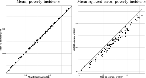
Figure 1: On the left, means $\times$100 over simulated populations of HB estimates of poverty incidence $F_{0d}$ against the analogous means for EB estimates, for each area $d$. On the right, mean squared errors ${\times}$10⁴ of HB estimators against those of EB estimators.

The left panel of Figure 1 displays means over Monte Carlo replicates of HB estimates of poverty incidences for each area against corresponding means of EB estimates. The right panel gives the frequentist mean squared errors of HB estimates against those of EB estimates for each area. Thus, from a frequentist point of view, we can see that the two estimators are practically the same, probably because only noninformative priors have been considered. The true mean squared errors of EB estimators are slightly smaller than those of HB estimates, which is somewhat sensible since the EB estimates are approximately the best under the frequentist paradigm. Figure 2 shows similar results for the poverty gap. Both figures show that the HB estimates display good frequentist properties.

In addition to point estimates, the HB approach can also deliver credible intervals. It is interesting to see whether these intervals satisfy the basic frequentist property of covering the true value. The left panel of Figure 3 displays the frequentist coverage of 95% credible intervals for the area poverty incidences, calculated as a percentage of Monte Carlo replicates in which credible intervals contain true values. We have plotted the coverages of equal tails credible intervals together with those of highest probability density intervals [Chen and Shao (1999)]. This figure reveals a slight undercoverage of less than 1% for the two types of intervals. The estimated coverage of credible intervals with only $H=1000$ replicates might not be very accurate, so we guess that a larger $H$ could show a smaller undercoverage. On the right panel of the same figure we report the mean widths of the two types of intervals. As expected, the highest posterior density intervals are clearly narrower. Similar conclusions can be drawn from Figure 4 for the poverty gap.

Figure 2: On the left, means $\times$100 over simulated populations of HB estimators of the poverty gap $F_{1d}$ against the analogous means for EB estimators, for each area $d$. On the right, mean squared errors ${\times}$10⁴ of HB estimators against those of EB estimators.

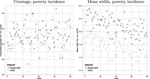
Figure 3: Percent coverage, left panel, and mean widths, right panel, over Monte Carlo populations of equal tails and highest posterior density intervals for poverty incidence $F_{0d}$ for each area $d$.

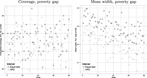
Figure 4: Percent coverage, left panel, and mean widths, right panel, over Monte Carlo populations of equal tails and highest posterior density credible intervals for poverty gap $F_{1d}$ for each area $d$.

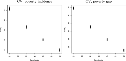
Figure 5: Mean over Monte Carlo simulations of CVs of HB estimators of poverty incidence (left panel) and poverty gap (right panel).

Finally, to analyze the effect of the sample size on the performance of the HB estimators, a new simulation experiment was conducted with increasing area sample sizes $n_{d}$ in the set $\{20,30,40,50\}$, with each value repeated for 20 areas and with a total number of areas $D=20\times 4=80$ as before. In this experiment we omitted the covariates that could distort the results and consider only a mean model with intercept $\bolds{\beta}_{0}=3$ as before. Figure 5 plots the mean coefficients of variation (CVs) of HB estimators of poverty incidences and poverty gaps. The estimated CV of an HB estimator is taken as the square root of the posterior variance divided by the estimate. Observe that, on average, the CVs increase about 3% when decreasing the area sample size in 10 units. Moreover, in this simulated example, it turns out that at least $n_{d}=50$ units need to be observed in area $d$ to keep the CV of HB estimators of poverty incidences below 20%. For the poverty gap, which is more difficult to estimate, the same sample size ensures a maximum CV of 25%.

6 Poverty mapping in Spain

This section describes an application of the proposed HB method to poverty mapping in Spanish provinces by gender. The data come from the SILC conducted in Spain in year 2006 and is the same used by Molina and Rao (2010). The SILC collects microdata on income, poverty, social exclusion and living conditions, in a timely and comparable way across European Union (EU) countries. The results of this survey are then used for the structural indicators of social cohesion such as poverty incidence, income quintile share ratio and gender pay gap. Indeed, equality between women and men is one of the EU’s founding values; see, for example, http://ec.europa.eu/justice/gender-equality/. Thus, the EU is especially concerned about gender issues, fostering research devoted to the quantification or measurement of equality. For example, one of the commitments of the SAMPLE project funded by the European Commission (http://www.sample-project.eu/) was to obtain poverty indicators in Spanish provinces by gender.

The Spanish SILC survey design is as follows. An independent sample is drawn from each of the Spanish Autonomous Communities using a two-stage design with stratification of the first stage units. The first stage or primary sampling units are census tracks and they are grouped into strata according to the size of the municipality where the census track is located. Census tracks are drawn within each stratum with probability proportional to their size. The secondary sampling units are main family dwellings, which are selected with equal probability and with random start systematic sampling. Within those last stage units, all individuals with usual residence in the dwelling are interviewed. This procedure results in self-weighted samples within each stratum. This survey is planned to provide reliable estimates only for the overall Spain and for the Autonomous Communities which are large Spanish regions, but it cannot deliver efficient estimates for the Spanish provinces disaggregated by gender due to the small sample size (provinces are nested within Autonomous Communities). Therefore, small area estimation techniques that “borrow strength” from other provinces are needed. The HB methodology proposed in this paper allows us to produce efficient estimates of practically any poverty indicator for the Spanish provinces by gender, using a computationally fast procedure, and provides at the same time all pertinent output such as uncertainty measures and credible intervals.

In this application, the target domains are the $D=52$ Spanish provinces. Since many studies on poverty in developing countries point to more severe levels of poverty for females than for males, it is very important to analyze if this happens in Spain as well. Thus, we are interested in giving estimates also by gender. To this end, we applied the HB procedure described in Section 5 separately for each gender, obtaining estimates of poverty incidences and gaps for the Spanish provinces, together with 95% highest posterior density intervals. The HB procedure was applied with a grid of $R=1000$ values of $\rho$ and $H=1000$ Monte Carlo replicates. For comparison, the EB method of Molina and Rao (2010) was also applied separately for each gender. Since this method is computationally slower, we considered only $L=50$ Monte Carlo simulations as in Molina and Rao (2010). The parametric bootstrap approach proposed in the same paper for mean squared error (MSE) estimation of EB estimates was applied with $B=200$ bootstrap replicates.

The overall sample size is 16,650 for males and 17,739 for females. The population size is 21,285,431 for males and 21,876,953 for females, with a total population size of over 43 million. We considered the same auxiliary variables as in Molina and Rao (2010), namely, the indicators of five quinquennial age groups, of having Spanish nationality, of the three levels of the variable education level, and of the three categories of the variable labor force status, “unemployed,” “employed” and “inactive.” For each auxiliary variable, one of the categories was considered as base reference, omitting the corresponding indicator and including an intercept in the model.

When making use of continuous covariates, all the methods (HB, EB and WB) require a full census of those covariates. In this application, however, only dummy indicators were included in the model and, therefore, only the counts of people with the same vector of $x$-values are needed. However, to make the computations as general as possible, we imitated the case of having continuous covariates by constructing the full census matrices $\mathbf{X}_{d}=(\mathbf{x}_{d1},\ldots,\mathbf{x}_{dN_{d}})^{\prime}$. This was done using the data from the Spanish Labour Force Survey (LFS), which has a much larger sample size than the SILC (155,333 as compared with 34,389) and therefore offers information with much better quality. Each LFS vector $\mathbf{x}_{di}^{\prime}$ was replicated a number of times equal to its corresponding LFS sampling weight; the resulting matrix $\mathbf{X}_{d}$ may be treated as a proxy of the true census matrix. As noted in Section 1, the WB was able to secure true census matrices $\mathbf{X}_{d}$ from statistical offices of many countries.

The welfare variable provided by the SILC for each individual and used to measure poverty by the Spanish Statistical Institute (INE in Spanish) and also by the European Statistical Office Eurostat is the so-called equivalized annual net income, which is the household annual net income, divided by a measure of household size calculated according to the scale defined by the OCDE. The resulting quantity can be interpreted as a kind of per capita income and for this reason it is assigned to each household member. Using instead the total household income would require the definition of a different poverty line for each possible household size and would not allow us to estimate by gender. For this reason, in this application we consider that the units are the individuals and, as welfare measure $E_{di}$, we consider the equivalized annual net income. Due to the clear right skewness of the histogram of $E_{di}$ values, we consider the transformation $Y_{di}=T(E_{di})=\log(E_{di}+c)$, where $c\geq\max\{0,-\min(E_{dj})+1\}$ is a constant selected in such a way that all shifted incomes $E_{di}+c$ are positive (there are few negative $E_{di}$) and for which the distribution of model residuals is closest to being symmetric. To select $c$, we took a grid of points in the range of income values and the model was fitted for each point in the grid. Then $c$ was selected as the point in this grid for which Fisher’s asymmetry coefficient of model residuals (third order centered sample moment divided by the cube standard deviation) was closest to zero. It turned out to be exactly the same value in the two models for Males and Females.

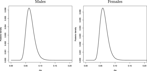
Figure 6: Posterior density of $\rho$ in the model for males, left panel, and females, right panel, obtained drawing from a grid in $[\varepsilon,1-\varepsilon]$ with $\varepsilon=0.0001$.

Figure 7: Histograms of posterior distributions of poverty incidences, upper panel, and poverty gaps, lower panel, for areas $d=1,2,3,4$, respectively, in columns, for females.

Since samples are drawn independently for each of the 18 Autonomous Communities and these regions might have different socio-economic levels, trying to accommodate the sampling design, we also fitted a model with Autonomous Community effects. However, the goodness of fit of the model including these effects, as measured by AIC and BIC, became worse for the two genders. Thus, we consider a more parsimonious model without Autonomous Community effects.

Figure 6 shows the posterior density of the intraclass correlation $\rho$ obtained in the models for males and females, using a grid of 5000 values of $\rho$ in the interval $[0.0001,0.9999]$. The two plots show that the mass of the posterior density of $\rho$ is mostly concentrated in $[0.04,0.1]$ and, therefore, the use of the truncation point $\varepsilon=0.0001$ in the two extremes of the range of $\rho$ to ensure a proper posterior does not have any effect in this application. In fact, trying to analyze the sensitivity to varying $\varepsilon$, we also used $\varepsilon=0.001$ and $\varepsilon=0.005$ and we found virtually no difference in the resulting posterior densities of $\rho$.

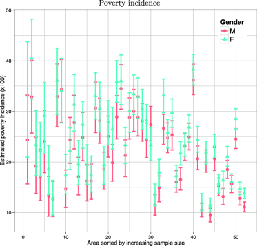
Figure 8: Hierarchical Bayes estimates of poverty incidences with highest posterior density intervals for each gender and for each area $d$. Areas are sorted by increasing sample size.

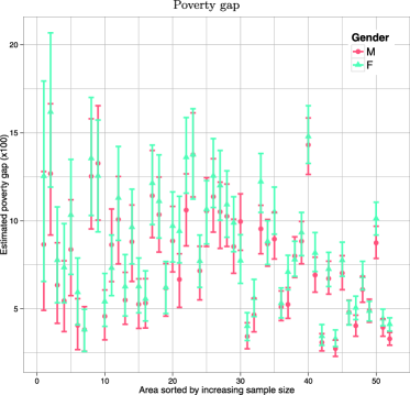
Figure 9: Hierarchical Bayes estimates of poverty gaps with highest posterior density intervals for each gender and for each area $d$. Areas are sorted by increasing sample size.

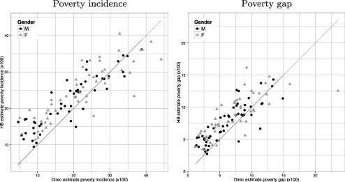
Figure 10: Hierarchical Bayes estimates of poverty incidence $F_{0d}$, left panel, and of poverty gap $F_{1d}$, right panel, against direct estimates for each province $d$.

Figure 7 shows the histograms of the posterior distributions of poverty incidences, upper panel, and poverty gaps, lower panel, for the first 4 provinces in the alphabetical order, in the model for females. Note that these histograms are slightly skewed. Therefore, we considered highest posterior density intervals instead of credible intervals with equal probability tails. These intervals were computed as described in Chen and Shao (1999). Figure 8 plots HB estimates of poverty incidences together with their corresponding 95% highest posterior density intervals for each gender and for each province, with areas sorted by increasing sample size. This figure shows that the length of the intervals decreases as the area sample sizes increase, as expected. It also shows that the estimated poverty incidences for males are smaller than for females for most provinces, although the two corresponding intervals cross each other for practically all provinces. Concerning the poverty gap, which measures the degree of poverty instead of the frequency of poor, Figure 9 shows a very similar pattern, with point estimates for females larger than for males in most provinces.

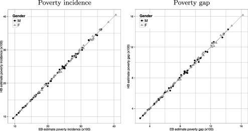
Figure 11: Hierarchical Bayes estimates of poverty incidence $F_{0d}$, left panel, and of poverty gap $F_{1d}$, right panel, against EB estimates for each province $d$.

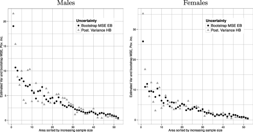
Figure 12: Posterior variances of HB estimators and bootstrap mean squared errors of EB estimators of poverty incidence for each province for males, left panel, and females, right panel. Provinces sorted by increasing sample size.

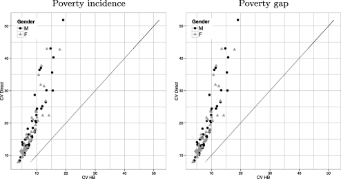
Figure 13: Coefficients of variation of direct estimates of poverty incidence $F_{0d}$, left panel, and of poverty gap $F_{1d}$, right panel, against coefficients of variation of HB estimates for each province $d$.

Figure 10 plots HB estimates of poverty incidence, left panel, and of poverty gap, right panel, against direct estimates for each area $d$, using separate plotting symbols for each gender. Observe that all points lie around the line, except for one of them corresponding to the poverty gap for women. This point is separated from the line because its direct estimate is much larger than the HB estimate. This occurs because HB estimates shrink extreme direct estimates toward synthetic regression ones for areas with small sample size.

Figure 11 plots HB estimates of poverty incidence, left panel, and of poverty gap, right panel, against EB estimates for each gender and for each province. Observe that HB estimates are practically equal to the corresponding EB estimates. Thus, in this application the point estimates obtained by the HB method proposed in this paper agree to a great extent with those obtained by the EB method.

Turning to the measures of variability of EB and HB estimators, Figure 12 compares the estimated MSEs of the EB estimators obtained by the parametric bootstrap described in Molina and Rao (2010), with the posterior variances. Although in principle these measures are not strictly comparable, it is interesting to see their similarity, and this similarity increases for areas with larger sample sizes.

Concerning computational efficiency, in this application, the full EB procedure consisting in the Monte Carlo approximation of the EB estimator with $L=50$ Monte Carlo replicates and the bootstrap method for MSE estimation with $B=200$ bootstrap replicates took 44.2 hours in a 2.67 GHz PC, whereas the HB procedure takes 3.7 hours. If we wanted the bootstrap MSE estimates to have comparable precision as the HB posterior variances and take $B=H=1000$ bootstrap replicates, the computational time of the full EB method in this application would be over 9 nonstop days on the same computer. Use of double bootstrap for bias reduction of the bootstrap MSE estimator would increase the computational complexity manyfold. Thus, for a larger number of auxiliary variables $p$, larger population size or a more complex indicator, computational times might be considerable for the EB method and in those cases the HB method represents a much faster alternative.

To see more clearly the efficiency gain of the HB estimates over direct estimates, in Figure 13 we plot the estimated CVs of direct estimators against those of HB estimators for all provinces. Observe that the CVs of direct estimators are above the 45^∘ line for all the provinces, indicating that HB estimates are more precise than direct estimates for all the provinces. Moreover, the gains are larger for provinces with smaller sample sizes and can be considerably large for some of the provinces. In contrast, the results obtained by Molina and Morales (2009) under an area-level model using the aggregated values of the same covariates provided only marginal reductions in the CVs over direct estimates.

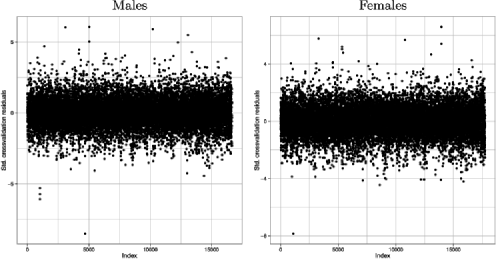
Figure 14: Index plot of standardized residuals for males, left panel, and females, right panel.

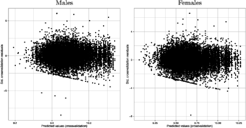
Figure 15: Standardized residuals against predicted values by cross-validation, for males, left panel, and females, right panel.

We have also done some diagnostic checks of the model assumptions using the cross-validation residuals $r_{di}$ introduced in (9). Index plots of residuals for males and females are included in Figure 14. In Figure 15 we show the plots of standardized cross-validation residuals against predicted values. The points that appear aligned at the bottom correspond to a number of zero incomes. Apart from this fact, we can see that the plots look acceptable without any visible pattern. Concerning CPOs, Figure 16 plots these validation measures against observed values $Y_{di}$ for males and females. As expected, there is high predicted power near the center of the data. The percentage of observations with CPO values below 0.025 turns out to be 1.5% for females and 1.2% for males, and the percentage below 0.014 (extreme outliers) is 0.9% for females and 0.8% for males. These results do not show any indication of serious departure from model assumptions; see Ntzoufras (2009).

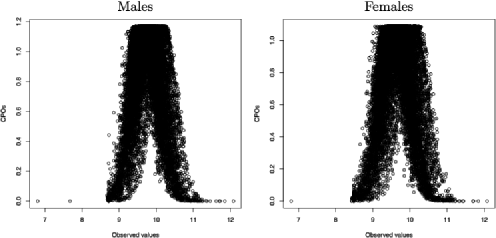
Figure 16: CPOs against observed values $Y_{di}$ for males, left panel, and females, right panel.

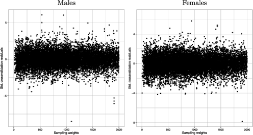
Figure 17: Standardized residuals against sampling weights in the range 0–2000, for males, left panel, and females, right panel.

Note that in this method, as in any other small area estimation procedure based on a unit-level model, the model is assumed not only for the sample units but also for the out-of-sample units. This assumption is reasonable as long as the design is noninformative, that is, the inclusion probabilities of the units in the sample are not related to the study variable (income) after accounting for the auxiliary variables. The SILC data contains the sampling weights or inverses of inclusion probabilities corrected for calibration and nonresponse. If the design is informative, model residuals should be related somehow with sampling weights. Thus, to analyze whether there is any evidence of informative sampling, in Figure 17 we have plotted cross-validation residuals $r_{di}$ versus sampling weights for males (left) and females (right) in the range 0–2000. There are sampling weights greater than 2000, but since the distribution is clearly right skewed with less large weights, for clarity of the plots we have plotted here the main part of the distribution. The null pattern of these plots indicate no evidence of informative sampling in this application.

Table 2 reports results obtained from the estimation of the poverty incidence, for provinces with sample sizes closest to minimum, first quartile, median, third quartile and maximum, for females and males. See that the posterior coefficient of variation is below 20% even for the area with smallest sample size, the province of Soria. Table 2 shows the corresponding results for the poverty gap, where the maximum coefficient of variation is below 25%.

== Males Females Province $\bolds{n_{d}}$ $\bolds{\hat{F}_{0d}^{\mathrm{HB}}}$ $\bolds{\mathrm{ll}(F_{0d})}$ $\bolds{\mathrm{ul}(F_{0d})}$ $\bolds{\mathrm{cv}(\hat{F}_{0d}^{\mathrm{HB}})}$ Province $\bolds{n_{d}}$ $\bolds{\hat{F}_{0d}^{\mathrm{HB}}}$ $\bolds{\mathrm{ll}(F_{0d})}$ $\bolds{\mathrm{ul}(F_{0d})}$ $\bolds{\mathrm{cv}(\hat{F}_{0d}^{\mathrm{HB}})}$ Soria $24$ $24.4$ $15.7$ $33.2$ $19.1$ Soria $17$ $33.2$ $21.0$ $43.8$ $17.9$ Lérida $127$ $24.8$ $20.3$ $29.8$ $9.9$ Gerona $138$ $17.4$ $14.1$ $21.2$ $10.7$ Jaén $233$ $28.8$ $25.1$ $33.0$ $7.1$ Ciudad Real $239$ $30.5$ $26.4$ $34.4$ $6.7$ Las Palmas $458$ $25.0$ $22.4$ $27.7$ $5.4$ Sevilla $491$ $24.4$ $22.0$ $27.0$ $5.4$ Barcelona $1358$ $11.1$ $10.2$ $12.1$ $4.5$ Barcelona $1483$ $13.8$ $12.8$ $14.8$ $3.8$ == Males Females Province $\bolds{n_{d}}$ $\bolds{\hat{F}_{1d}^{\mathrm{HB}}}$ $\bolds{\mathrm{ll}(F_{1d})}$ $\bolds{\mathrm{ul}(F_{1d})}$ $\bolds{\mathrm{cv}(\hat{F}_{1d}^{\mathrm{HB}})}$ Province $\bolds{n_{d}}$ $\bolds{\hat{F}_{1d}^{\mathrm{HB}}}$ $\bolds{\mathrm{ll}(F_{1d})}$ $\bolds{\mathrm{ul}(F_{1d})}$ $\bolds{\mathrm{cv}(\hat{F}_{1d}^{\mathrm{HB}})}$ Soria $24$ $8.7$ $4.9$ $12.8$ $24.5$ Soria $17$ $12.5$ $6.6$ $17.9$ $24.0$ Lérida $127$ $8.8$ $6.6$ $10.9$ $12.7$ Gerona $138$ $5.6$ $4.3$ $7.2$ $13.3$ Jaén $233$ $10.5$ $8.4$ $12.2$ $9.3$ Ciudad Real $239$ $10.9$ $9.1$ $12.8$ $8.9$ Las Palmas $458$ $8.8$ $7.6$ $10.0$ $7.0$ Sevilla $491$ $8.2$ $7.1$ $9.3$ $7.0$ Barcelona $1358$ $3.3$ $2.9$ $3.7$ $5.5$ Barcelona $1483$ $4.1$ $3.7$ $4.5$ $4.8$

Table 1: Sample size, HB estimates of poverty incidence $\times$100, lower and upper limits of highest posterior density intervals and coefficients of variation of HB estimates for the Spanish provinces with sample size closest to minimum, first quartile, median, third quartile and maximum, for each gender

Table 2: Sample size, HB estimates of poverty gap $\times$100, lower and upper limits of highest posterior density intervals and coefficients of variation of HB estimates for the Spanish provinces with sample size closest to minimum, first quartile, median, third quartile and maximum, for each gender

Finally, the point estimates of poverty incidence and poverty gap obtained using the HB procedure are plotted in the cartograms of Figures 18 and 19, for females and males. Although the method has been applied separately for each gender in contrast to the application done in Molina and Rao (2010) which treats provinces crossed with gender as domains, we can see that the maps are very similar.

7 Discussion

The proposed HB procedure gives efficient estimates of general nonlinear parameters in small areas using a model for unit-level data. It is a computationally faster alternative to the EB method of Molina and Rao (2010) and at the same time it provides a full description of the posterior distribution of the target parameters, making it very easy to construct credible intervals or to obtain other posterior summaries. The frequentist simulation study described in Section 5 and the application with Spanish SILC data given in Section 6 indicate that HB point estimates agree to a great extent with EB estimates and that posterior variances are also comparable with frequentist MSEs. This good property arises from the fact of using only noninformative priors. Thus, the proposed HB method is in practice more feasible than the EB method for the estimation of general nonlinear indicators under large populations.

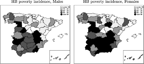
Figure 18: Cartograms of estimated percent poverty incidences in Spanish provinces for men and women, obtained using the HB method. Canary islands have been moved to the bottom-right corner.

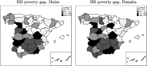
Figure 19: Cartograms of estimated percent poverty gaps in Spanish provinces for men and women, obtained using the HB method. Canary islands have been moved to the bottom-right corner.

In addition, the proposed HB approach provides estimators of poverty indicators in Spanish provinces that are considerably more efficient than direct estimators; see Figure 13. Results highlight larger point estimates of poverty incidence and poverty gap for females in almost all provinces although credible intervals for the two genders cross each other.

According to the resulting poverty maps, poverty (both in frequency and intensity) is mainly concentrated in the south and west of Spain. Provinces with critical estimated poverty incidences for men, with at least 30% of people under the poverty line, are Almería, Badajoz, Albacete, Cuenca, Ávila and Zamora. For women, almost all provinces get a larger point estimate of poverty incidence. In particular, many more provinces join the set of provinces with critical values, namely, practically all provinces in the region of Andalucía except for Sevilla and Cádiz, all the provinces in Castilla la Mancha region except for Toledo and two more provinces in Castilla León. Lleida in the north–east (region of Catalonia) obtains a worrying poverty incidence for women as compared with the rest of the provinces in the same region. In Spain the frequency of poverty as measured by the poverty incidence seems to be very much related with the intensity of poverty as measured by the poverty gap, with maps for the poverty gaps showing a similar distribution of the poverty across provinces.

In contrast to the case of estimating area means or totals, the proposed method, as any other unit-level method for estimating nonlinear parameters, requires the values of the auxiliary variables for each population unit instead of area aggregates. These data can be obtained from the last census or from administrative registers. But due to confidentiality issues and depending on the particular regulation of each country, census data might not be easily available for practitioners beyond statistical offices personnel. In some other countries, access to census data can be obtained by prior signature of strict data protection contracts. In other small area applications, such as, for example, agriculture or forest research, the population of $x$-values is fully available to the researcher from satellite or laser sensors images [Battese, Harter and Fuller (1988); Breidenbach and Astrup (2012)].

A model with spatial correlation among provinces might be considered, but there are serious difficulties in defining boundary conditions, especially for several provinces such as islands. Even if spatial correlation could be considered for a subset of the provinces, the number of provinces left is not large enough to estimate accurately the spatial correlation, leading to weak significance of this parameter. An area-level model with spatial correlation among Spanish provinces is studied by Marhuenda, Molina and Morales (2013), and their results for the SILC data indicated very mild gains in efficiency due to the introduction of the spatial correlation in the model. In any case, we leave this for further research.

Appendix A Derivation of posterior densities

Here we derive the conditional distributions appearing on the right-hand side of the chain rule in (3). By Bayes’ theorem and using model assumptions (2)–(3) together with the prior (4), the posterior distribution is given by

$$\pi\bigl{(}\mathbf{u},\bolds{\beta},\sigma^{2},\rho|\mathbf{y}_{s}\bigr{)}$$

$$\qquad\propto\Biggl{\{}\prod_{d=D^{*}+1}^{D}\pi\bigl{(}u_{d}|\bolds{\beta},\sigma^{2},\rho\bigr{)}\Biggr{\}}\biggl{(}\frac{1-\rho}{\rho}\biggr{)}^{D^{*}/2}\bigl{(}\sigma^{2}\bigr{)}^{-(((D^{*}+n)/2)+1)}$$ (11)

$$\quad\qquad{}\times\exp\Biggl{\{}-\frac{1}{2\sigma^{2}}\sum_{d=1}^{D^{*}}\biggl{[}\sum_{i\in s_{d}}w_{di}\bigl{(}Y_{di}-\mathbf{x}_{di}^{\prime}\bolds{\beta}-u_{d}\bigr{)}^{2}+\frac{1-\rho}{\rho}u_{d}^{2}\biggr{]}\Biggr{\}},$$

where $\pi(u_{d}|\bolds{\beta},\sigma^{2},\rho)$ is the normal prior of $u_{d}$ given in (3). Let us define the weighted sample means

$$\bar{\mathbf{x}}_{d}=\frac{1}{w_{d\cdot}}\sum_{i\in s_{d}}w_{di}\mathbf{x}_{di},\qquad\bar{y}_{d}=\frac{1}{w_{d\cdot}}\sum_{i\in s_{d}}w_{di}Y_{di},$$

where $w_{d\cdot}=\sum_{i\in s_{d}}w_{di}$, $d=1,\ldots,D^{*}$. Integrating out $\mathbf{u}$ in (A), we obtain $\pi(\bolds{\beta},\sigma^{2},\rho|\mathbf{y}_{s})$. Now dividing $\pi(\mathbf{u},\bolds{\beta},\sigma^{2},\rho|\mathbf{y}_{s})$ by $\pi(\bolds{\beta},\sigma^{2},\rho|\mathbf{y}_{s})$, we obtain

$$\pi\bigl{(}\mathbf{u}|\bolds{\beta},\sigma^{2},\rho,\mathbf{y}_{s}\bigr{)}=\Biggl{\{}\prod_{d=D^{*}+1}^{D}\pi\bigl{(}u_{d}|\bolds{\beta},\sigma^{2},\rho\bigr{)}\Biggr{\}}\Biggl{\{}\prod_{d=1}^{D^{*}}\pi\bigl{(}u_{d}|\bolds{\beta},\sigma^{2},\rho,\mathbf{y}_{s}\bigr{)}\Biggr{\}},$$

where

$$u_{d}|\bolds{\beta},\sigma^{2},\rho,\mathbf{y}_{s}\stackrel{{\scriptstyle\mathrm{ind}}}{{\sim}}N\biggl{[}\lambda_{d}(\rho)\bigl{(}\bar{y}_{d}-\bar{\mathbf{x}}_{d}^{\prime}\bolds{\beta}\bigr{)},\bigl{\{}1-\lambda_{d}(\rho)\bigr{\}}\frac{\rho}{1-\rho}\sigma^{2}\biggr{]}$$ (12)

for $\lambda_{d}(\rho)=w_{d\cdot}[w_{d\cdot}+(1-\rho)/\rho]^{-1}$, $d=1,\ldots,D^{*}$. The second conditional density $\pi_{2}(\bolds{\beta}|\sigma^{2},\rho,\mathbf{y}_{s})$ in (3) is obtained by integrating out $\bolds{\beta}$ in $\pi(\bolds{\beta},\sigma^{2},\rho|\mathbf{y}_{s})$ and then dividing $\pi(\bolds{\beta},\sigma^{2},\rho|\mathbf{y}_{s})$ by $\pi(\sigma^{2},\rho|\mathbf{y}_{s})$. Let

$$\mathbf{Q}(\rho) = \sum_{d=1}^{D^{*}}\sum_{i\in s_{d}}w_{di}(\mathbf{x}_{di}-\bar{\mathbf{x}}_{d})(\mathbf{x}_{di}-\bar{\mathbf{x}}_{d})^{\prime}+\frac{1-\rho}{\rho}\sum_{d=1}^{D^{*}}\lambda_{d}\bar{\mathbf{x}}_{d}\bar{\mathbf{x}}_{d}^{\prime},$$

$$\mathbf{p}(\rho) = \sum_{d=1}^{D^{*}}\sum_{i\in s_{d}}w_{di}(\mathbf{x}_{di}-\bar{\mathbf{x}}_{d})(Y_{di}-\bar{y}_{d})+\frac{1-\rho}{\rho}\sum_{d=1}^{D^{*}}\lambda_{d}\bar{\mathbf{x}}_{d}\bar{y}_{d}$$

and $\hat{\bolds{\beta}}(\rho)=\mathbf{Q}^{-1}(\rho)\mathbf{p}(\rho)$. Then, it follows that

$$\bolds{\beta}|\sigma^{2},\rho,\mathbf{y}_{s}\sim N\bigl{\{}\hat{\bolds{\beta}}(\rho),\sigma^{2}\mathbf{Q}^{-1}(\rho)\bigr{\}}.$$ (13)

Finally, integrating out $\sigma^{2}$ in $\pi(\sigma^{2},\rho|\mathbf{y}_{s})$, we obtain

$$\pi_{4}(\rho|\mathbf{y}_{s})\propto\biggl{(}\frac{1-\rho}{\rho}\biggr{)}^{D^{*}/2}\bigl{|}\mathbf{Q}(\rho)\bigr{|}^{-1/2}\gamma(\rho)^{-(n-p)/2}\prod_{d=1}^{D^{*}}\lambda_{d}^{1/2}(\rho),$$

(14)

$$\eqntext{\varepsilon\leq\rho\leq 1-\varepsilon,}$$ (15)

where

$$\gamma(\rho) = \sum_{d=1}^{D^{*}}\sum_{i\in s_{d}}w_{di}\bigl{\{}Y_{di}-\bar{y}_{d}-(\mathbf{x}_{di}-\bar{\mathbf{x}}_{d})^{\prime}\hat{\bolds{\beta}}(\rho)\bigr{\}}^{2}$$

$${}+\frac{1-\rho}{\rho}\sum_{d=1}^{D^{*}}\lambda_{d}(\rho)\bigl{\{}\bar{y}_{d}-\bar{\mathbf{x}}_{d}^{\prime}\hat{\bolds{\beta}}(\rho)\bigr{\}}^{2}.$$

Dividing $\pi(\sigma^{2},\rho|\mathbf{y}_{s})$ by $\pi_{4}(\rho|\mathbf{y}_{s})$ and making a change of variable, we finally obtain

$$\sigma^{-2}|\rho,\mathbf{y}_{s}\sim\operatorname{Gamma}\biggl{(}\frac{n-p}{2},\frac{\gamma(\rho)}{2}\biggr{)}.$$ (16)

Appendix B Propriety of the posterior distribution

Lemma 1.

Under the model defined by (2), (3) and (4), the posterior density $\pi(\mathbf{u},\bolds{\beta},\sigma^{2},\rho\mid\mathbf{y}_{s})$ is proper provided that the matrix defined by stacking the rows $\mathbf{x}_{di}^{\prime}$ in columns, $X=\mathrm{col}_{1\leq d\leq D}\mathrm{col}_{i\in s_{d}}(\mathbf{x}_{di}^{\prime})$, has full column rank and $\varepsilon\leq\rho\leq 1-\varepsilon,\varepsilon>0$.

We need to show that $\int\!\!\int\!\!\int\!\!\int\pi(\mathbf{u},\bolds{\beta},\sigma^{2},\rho|\mathbf{y}_{s})\,d\mathbf{u}\,d\bolds{\beta}\,d\sigma^{2}\,\mathbf{d}\rho$ is finite, where the posterior $\pi(\mathbf{u},\bolds{\beta},\sigma^{2},\rho|\mathbf{y}_{s})$ is given in (3); see also Appendix A.

Now, using the expression for the posterior given in (3), the integral of the posterior distribution is given by

$$\int\!\!\int\!\!\int\!\!\int\pi\bigl{(}\mathbf{u},\bolds{\beta},\sigma^{2},\rho|\mathbf{y}_{s}\bigr{)}\,d\mathbf{u}\,d\bolds{\beta}\,\mathbf{d}\sigma^{2}\,\mathbf{d}\rho$$

$$\qquad=\int\biggl{[}\int\biggl{\{}\int\biggl{(}\int\pi_{1}\bigl{(}\mathbf{u}|\bolds{\beta},\sigma^{2},\rho,\mathbf{y}_{s}\bigr{)}\,d\mathbf{u}\biggr{)}\pi_{2}\bigl{(}\bolds{\beta}|\sigma^{2},\rho,\mathbf{y}_{s}\bigr{)}\,d\bolds{\beta}\biggr{\}}$$

$$\hskip 192.0pt{}\times\pi_{3}\bigl{(}\sigma^{2}|\rho,\mathbf{y}_{s}\bigr{)}\,d\sigma^{2}\biggr{]}\pi_{4}(\rho|\mathbf{y}_{s})\,d\rho.$$

Here $\pi_{1}(\mathbf{u}|\bolds{\beta},\sigma^{2},\rho,\mathbf{y}_{s})=\prod_{d=1}^{D}\pi_{1d}(u_{d}|\bolds{\beta},\sigma^{2},\rho,\mathbf{y}_{s})$, and the distribution of $u_{d}|\bolds{\beta},\sigma^{2},\rho,\mathbf{y}_{s}$ is given by (12), which is proper (integrates to one), because $\rho\in[\varepsilon,1-\varepsilon]$ for $\varepsilon>0$. Similarly, the distribution of $\bolds{\beta}|\sigma^{2},\rho,\mathbf{y}_{s}$ is given in (13), where the inverse of $Q(\rho)$ exists whenever $\rho\in[\varepsilon,1-\varepsilon]$ for $\varepsilon>0$ and $X$ has full column rank. Concerning $\sigma^{2}$, the density of $\sigma^{-2}|\rho,\mathbf{y}_{s}$ is given in (16). Making the change of variable $v=\sigma^{-2}$, we obtain $\int\pi_{3}(\sigma^{2}|\rho,\mathbf{y}_{s})\,d\sigma^{2}=1$.

Finally, we note that $\rho$ cannot be integrated out analytically because the posterior of $\rho$ is given up to a constant by (A). However,

$$\int_{\varepsilon}^{1-\varepsilon}\biggl{(}\frac{1-\rho}{\rho}\biggr{)}^{D^{*}/2}\bigl{|}\mathbf{Q}(\rho)\bigr{|}^{-1/2}\gamma(\rho)^{-(n-p)/2}\prod_{d=1}^{D^{*}}\lambda_{d}^{1/2}(\rho)\,d\rho<\infty,$$

because the integrand is continuous for $\rho\in[\varepsilon,1-\varepsilon]$ provided that $X$ has full column rank.

Appendix C Computation of standardized cross-validation residuals

Following Gelfand, Dey and Chang (1992), the expectation of any function $g(Y_{di})$ can be expressed as

$$E\bigl{[}g(Y_{di})|\mathbf{y}_{s(di)}\bigr{]}$$

$$\qquad=\int E\bigl{[}g(Y_{di})|\mathbf{y}_{s(di)},\bolds{\theta}\bigr{]}\pi(\bolds{\theta}|\mathbf{y}_{s(di)})\,d\bolds{\theta}$$ (17)

$$\qquad\quad=\frac{\int E[g(Y_{di})|\mathbf{y}_{s(di)},\bolds{\theta}]((\pi(\bolds{\theta}|\mathbf{y}_{s(di)}))/(\pi(\bolds{\theta}|\mathbf{y}_{s})))\pi(\bolds{\theta}|\mathbf{y}_{s})\,d\bolds{\theta}}{\int((\pi(\bolds{\theta}|\mathbf{y}_{s(di)}))/(\pi(\bolds{\theta}|\mathbf{y}_{s})))\pi(\bolds{\theta}|\mathbf{y}_{s})\,d\bolds{\theta}}.$$

Now, to obtain the expectation $E(Y_{di}|\mathbf{y}_{s(di)})$, consider $g(x)=x$. The expectation within the integral in (C) is simply

$$E(Y_{di}|\mathbf{y}_{s(di)},\bolds{\theta})=E(Y_{di}|\bolds{\theta})=\mathbf{x}_{di}^{\prime}\bolds{\beta}+u_{d},$$

because, given $\bolds{\theta}$, all observations are independent and distributed as indicated in (6). Thus, if we generate $H$ values $\bolds{\theta}^{(h)}=((\mathbf{u}^{(h)})^{\prime},(\bolds{\beta}^{(h)})^{\prime},\sigma^{2(h)},\rho^{(h)})^{\prime}$, $h=1,\ldots,H$, from the posterior density with all the data, $\pi(\bolds{\theta}|\mathbf{y}_{s})$, then the desired expectation would be obtained as

$$E(Y_{di}|\mathbf{y}_{s(di)})\approx\sum_{h=1}^{H}\bigl{(}\mathbf{x}_{di}^{\prime}\bolds{\beta}^{(h)}+u_{d}^{(h)}\bigr{)}v_{di}^{(h)},\qquad i\in s_{d},d=1,\ldots,D,$$

where

$$v_{di}^{(h)}=\Biggl{\{}\sum_{k=1}^{H}\frac{\pi(\bolds{\theta}^{(k)}|\mathbf{y}_{s(di)})}{\pi(\bolds{\theta}^{(k)}|\mathbf{y}_{s})}\Biggr{\}}^{-1}\frac{\pi(\bolds{\theta}^{(h)}|\mathbf{y}_{s(di)})}{\pi(\bolds{\theta}^{(h)}|\mathbf{y}_{s})}.$$

But by Bayes’ theorem, we have

$$\frac{\pi(\bolds{\theta}^{(h)}|\mathbf{y}_{s(di)})}{\pi(\bolds{\theta}^{(h)}|\mathbf{y}_{s})}=\frac{f(\mathbf{y}_{s(di)}|\bolds{\theta}^{(h)})}{f(\mathbf{y}_{s}|\bolds{\theta}^{(h)})}\frac{f(\mathbf{y}_{s})}{f(\mathbf{y}_{s(di)})}.$$

Therefore,

$$v_{di}^{(h)} = \frac{((f(\mathbf{y}_{s(di)}|\bolds{\theta}^{(h)}))/(f(\mathbf{y}_{s}|\bolds{\theta}^{(h)})))((f(\mathbf{y}_{s}))/(f(\mathbf{y}_{s(di)})))}{\sum_{k=1}^{H}((f(\mathbf{y}_{s(di)}|\bolds{\theta}^{(k)}))/(f(\mathbf{y}_{s}|\bolds{\theta}^{(k)})))((f(\mathbf{y}_{s}))/(f(\mathbf{y}_{s(di)})))}$$

$$= \frac{f(\mathbf{y}_{s(di)}|\bolds{\theta}^{(h)})\{f(\mathbf{y}_{s}|\bolds{\theta}^{(h)})\}^{-1}}{\sum_{k=1}^{H}f(\mathbf{y}_{s(di)}|\bolds{\theta}^{(k)})\{f(\mathbf{y}_{s}|\bolds{\theta}^{(k)})\}^{-1}}.$$

Now since, given $\bolds{\theta}$, all observations are independent, we have $f(\mathbf{y}_{s}|\bolds{\theta})=f(\mathbf{y}_{s(di)}|\bolds{\theta})f(Y_{di}|\bolds{\theta})$. Replacing this relation in $v_{di}^{(h)}$, we obtain the expression in (10).

References

- Battese, Harter and Fuller (1988) {barticle}[auto:STB—2014/01/06—10:16:28] \bauthor\bsnmBattese, \bfnmG. E.\binitsG. E., \bauthor\bsnmHarter, \bfnmR. M.\binitsR. M. and \bauthor\bsnmFuller, \bfnmW. A.\binitsW. A. (\byear1988). \btitleAn error-components model for prediction of county crop areas using survey and satellite data. \bjournalJ. Amer. Statist. Assoc. \bvolume83 \bpages28–36. \bptokimsref\endbibitem
- Bell (1997) {bmisc}[auto:STB—2014/01/06—10:16:28] \bauthor\bsnmBell, \bfnmW.\binitsW. (\byear1997). \bhowpublishedModels for county and state poverty estimates. Preprint, Statistical Research Division, U.S. Census Bureau, Washington, DC. \bptokimsref\endbibitem
- Berger (1985) {bbook}[mr] \bauthor\bsnmBerger, \bfnmJames O.\binitsJ. O. (\byear1985). \btitleStatistical Decision Theory and Bayesian Analysis, \bedition2nd ed. \bpublisherSpringer, \blocationNew York. \bidmr=0804611 \bptokimsref\endbibitem
- Betti et al. (2006) {bincollection}[auto:STB—2014/01/06—10:16:28] \bauthor\bsnmBetti, \bfnmG.\binitsG., \bauthor\bsnmCheli, \bfnmB.\binitsB., \bauthor\bsnmLemmi, \bfnmA.\binitsA. and \bauthor\bsnmVerma, \bfnmV.\binitsV. (\byear2006). \btitleMultidimensional and longitudinal poverty: An integrated fuzzy approach. In \bbooktitleFuzzy Set Approach to Multidimensional Poverty Measurement (\beditor\bfnmA.\binitsA. \bsnmLemmi and \beditor\bfnmG.\binitsG. \bsnmBetti, eds.) \bpages111–137. \bpublisherSpringer, \blocationNew York. \bptokimsref\endbibitem
- Box (1980) {barticle}[auto] \bauthor\bsnmBox, \bfnmG. E. P.\binitsG. E. P. (\byear1980). \btitleSampling and Bayes’ inference in scientific modelling and robustness (Discussion by Professor Seymour Geisser). \bjournalJ. Roy. Statist. Soc. Ser. A \bvolume143 \bpages416–417. \biddoi=10.2307/2982063, issn=0035-9238, mr=0603745 \bptokimsref\endbibitem
- Breidenbach and Astrup (2012) {barticle}[auto:STB—2014/01/06—10:16:28] \bauthor\bsnmBreidenbach, \bfnmJ.\binitsJ. and \bauthor\bsnmAstrup, \bfnmR.\binitsR. (\byear2012). \btitleSmall area estimation of forest attributes in the Norwegian national forest inventory. \bjournalEur. J. For. Res. \bvolume131 \bpages1255–1267. \bptokimsref\endbibitem
- Chen and Shao (1999) {barticle}[mr] \bauthor\bsnmChen, \bfnmMing-Hui\binitsM.-H. and \bauthor\bsnmShao, \bfnmQi-Man\binitsQ.-M. (\byear1999). \btitleMonte Carlo estimation of Bayesian credible and HPD intervals. \bjournalJ. Comput. Graph. Statist. \bvolume8 \bpages69–92. \biddoi=10.2307/1390921, issn=1061-8600, mr=1705909 \bptokimsref\endbibitem
- Datta (2009) {bincollection}[auto:STB—2014/01/06—10:16:28] \bauthor\bsnmDatta, \bfnmG. S.\binitsG. S. (\byear2009). \btitleModel-based approach to small area estimation. In \bbooktitleHandbook of Statistics 29A: Sample Surveys: Design, Methods and Applications (\beditor\bfnmD.\binitsD. \bsnmPfeffermann and \beditor\bfnmC. R.\binitsC. R. \bsnmRao, eds.) \bpages251–288. \bpublisherElsevier, \blocationAmsterdam. \bptokimsref\endbibitem
- Datta and Ghosh (1991) {barticle}[mr] \bauthor\bsnmDatta, \bfnmGauri Sankar\binitsG. S. and \bauthor\bsnmGhosh, \bfnmMalay\binitsM. (\byear1991). \btitleBayesian prediction in linear models: Applications to small area estimation. \bjournalAnn. Statist. \bvolume19 \bpages1748–1770. \biddoi=10.1214/aos/1176348369, issn=0090-5364, mr=1135147 \bptokimsref\endbibitem
- Elbers, Lanjouw and Lanjouw (2003) {barticle}[auto:STB—2014/01/06—10:16:28] \bauthor\bsnmElbers, \bfnmC.\binitsC., \bauthor\bsnmLanjouw, \bfnmJ. O.\binitsJ. O. and \bauthor\bsnmLanjouw, \bfnmP.\binitsP. (\byear2003). \btitleMicro-level estimation of poverty and inequality. \bjournalEconometrica \bvolume71 \bpages355–364. \bptokimsref\endbibitem
- Ferretti and Molina (2012) {barticle}[mr] \bauthor\bsnmFerretti, \bfnmCaterina\binitsC. and \bauthor\bsnmMolina, \bfnmIsabel\binitsI. (\byear2012). \btitleFast EB method for estimating complex poverty indicators in large populations. \bjournalJ. Indian Soc. Agricultural Statist. \bvolume66 \bpages105–120. \bidissn=0019-6363, mr=2953463 \bptokimsref\endbibitem
- Foster, Greer and Thorbecke (1984) {barticle}[auto:STB—2014/01/06—10:16:28] \bauthor\bsnmFoster, \bfnmJ.\binitsJ., \bauthor\bsnmGreer, \bfnmJ.\binitsJ. and \bauthor\bsnmThorbecke, \bfnmE.\binitsE. (\byear1984). \btitleA class of decomposable poverty measures. \bjournalEconometrica \bvolume52 \bpages761–766. \bptokimsref\endbibitem
- Gelfand, Dey and Chang (1992) {bincollection}[mr] \bauthor\bsnmGelfand, \bfnmA. E.\binitsA. E., \bauthor\bsnmDey, \bfnmD. K.\binitsD. K. and \bauthor\bsnmChang, \bfnmH.\binitsH. (\byear1992). \btitleModel determination using predictive distributions with implementation via sampling-based methods. In \bbooktitleBayesian Statistics, 4 (Peñíscola, 1991) \bpages147–167. \bpublisherOxford Univ. Press, \blocationNew York. \bidmr=1380275 \bptokimsref\endbibitem
- Jiang and Lahiri (2006) {barticle}[mr] \bauthor\bsnmJiang, \bfnmJiming\binitsJ. and \bauthor\bsnmLahiri, \bfnmP.\binitsP. (\byear2006). \btitleMixed model prediction and small area estimation. \bjournalTEST \bvolume15 \bpages1–96. \biddoi=10.1007/BF02595419, issn=1133-0686, mr=2252522 \bptnotecheck related \bptokimsref\endbibitem
- Marhuenda, Molina and Morales (2013) {barticle}[mr] \bauthor\bsnmMarhuenda, \bfnmYolanda\binitsY., \bauthor\bsnmMolina, \bfnmIsabel\binitsI. and \bauthor\bsnmMorales, \bfnmDomingo\binitsD. (\byear2013). \btitleSmall area estimation with spatio-temporal Fay–Herriot models. \bjournalComput. Statist. Data Anal. \bvolume58 \bpages308–325. \biddoi=10.1016/j.csda.2012.09.002, issn=0167-9473, mr=2997945 \bptokimsref\endbibitem
- Mohadjer et al. (2012) {barticle}[mr] \bauthor\bsnmMohadjer, \bfnmLeyla\binitsL., \bauthor\bsnmRao, \bfnmJ. N. K.\binitsJ. N. K., \bauthor\bsnmLiu, \bfnmBenmei\binitsB., \bauthor\bsnmKrenzke, \bfnmTom\binitsT. and \bauthor\bparticleVan de \bsnmKerckhove, \bfnmWendy\binitsW. (\byear2012). \btitleHierarchical Bayes small area estimates of adult literacy using unmatched sampling and linking models. \bjournalJ. Indian Soc. Agricultural Statist. \bvolume66 \bpages55–63, 232–233. \bidissn=0019-6363, mr=2953459 \bptokimsref\endbibitem
- Molina and Morales (2009) {barticle}[mr] \bauthor\bsnmMolina, \bfnmIsabel\binitsI. and \bauthor\bsnmMorales, \bfnmDomingo\binitsD. (\byear2009). \btitleSmall area estimation of poverty indicators. \bjournalBol. Estad. Investig. Oper. \bvolume25 \bpages218–225. \bidissn=1889-3805, mr=2751742 \bptokimsref\endbibitem
- Molina and Rao (2010) {barticle}[mr] \bauthor\bsnmMolina, \bfnmIsabel\binitsI. and \bauthor\bsnmRao, \bfnmJ. N. K.\binitsJ. N. K. (\byear2010). \btitleSmall area estimation of poverty indicators. \bjournalCanad. J. Statist. \bvolume38 \bpages369–385. \biddoi=10.1002/cjs.10051, issn=0319-5724, mr=2730115 \bptokimsref\endbibitem
- Nandram and Choi (2005) {barticle}[auto:STB—2014/01/06—10:16:28] \bauthor\bsnmNandram, \bfnmBalgobin\binitsB. and \bauthor\bsnmChoi, \bfnmJai Won\binitsJ. W. (\byear2005). \btitleHierarchical Bayesian nonignorable nonresponse regression models for small areas: An application to the NHNES data. \bjournalSurv. Methodol. \bvolume31 \bpages73–84. \bptokimsref\endbibitem
- Nandram and Choi (2010) {barticle}[mr] \bauthor\bsnmNandram, \bfnmBalgobin\binitsB. and \bauthor\bsnmChoi, \bfnmJai Won\binitsJ. W. (\byear2010). \btitleA Bayesian analysis of body mass index data from small domains under nonignorable nonresponse and selection. \bjournalJ. Amer. Statist. Assoc. \bvolume105 \bpages120–135. \biddoi=10.1198/jasa.2009.ap08443, issn=0162-1459, mr=2656046 \bptokimsref\endbibitem
- Nandram, Sedransk and Pickle (2000) {barticle}[mr] \bauthor\bsnmNandram, \bfnmBalgobin\binitsB., \bauthor\bsnmSedransk, \bfnmJ.\binitsJ. and \bauthor\bsnmPickle, \bfnmLinda Williams\binitsL. W. (\byear2000). \btitleBayesian analysis and mapping of mortality rates for chronic obstructive pulmonary disease. \bjournalJ. Amer. Statist. Assoc. \bvolume95 \bpages1110–1118. \biddoi=10.2307/2669747, issn=0162-1459, mr=1821719 \bptokimsref\endbibitem
- Natarajan and Kass (2000) {barticle}[mr] \bauthor\bsnmNatarajan, \bfnmRanjini\binitsR. and \bauthor\bsnmKass, \bfnmRobert E.\binitsR. E. (\byear2000). \btitleReference Bayesian methods for generalized linear mixed models. \bjournalJ. Amer. Statist. Assoc. \bvolume95 \bpages227–237. \biddoi=10.2307/2669540, issn=0162-1459, mr=1803151 \bptokimsref\endbibitem
- Neri, Ballini and Betti (2005) {barticle}[auto:STB—2014/01/06—10:16:28] \bauthor\bsnmNeri, \bfnmL.\binitsL., \bauthor\bsnmBallini, \bfnmF.\binitsF. and \bauthor\bsnmBetti, \bfnmG.\binitsG. (\byear2005). \btitlePoverty and inequality in transition countries. \bjournalStatistics in Transition \bvolume7 \bpages135–157. \bptokimsref\endbibitem
- Ntzoufras (2009) {bbook}[auto:STB—2014/01/06—10:16:28] \bauthor\bsnmNtzoufras, \bfnmI.\binitsI. (\byear2009). \btitleBayesian Modeling Using WinBUGS. \bpublisherWiley, \blocationHoboken, NJ. \bptokimsref\endbibitem
- Pettit (1990) {barticle}[mr] \bauthor\bsnmPettit, \bfnmL. I.\binitsL. I. (\byear1990). \btitleThe conditional predictive ordinate for the normal distribution. \bjournalJ. R. Stat. Soc. Ser. B Stat. Methodol. \bvolume52 \bpages175–184. \bidissn=0035-9246, mr=1049309 \bptokimsref\endbibitem
- Pfeffermann (2013) {barticle}[mr] \bauthor\bsnmPfeffermann, \bfnmDanny\binitsD. (\byear2013). \btitleNew important developments in small area estimation. \bjournalStatist. Sci. \bvolume28 \bpages40–68. \biddoi=10.1214/12-STS395, issn=0883-4237, mr=3075338 \bptokimsref\endbibitem
- Pfeffermann and Sverchkov (2007) {barticle}[mr] \bauthor\bsnmPfeffermann, \bfnmDanny\binitsD. and \bauthor\bsnmSverchkov, \bfnmMichail\binitsM. (\byear2007). \btitleSmall-area estimation under informative probability sampling of areas and within the selected areas. \bjournalJ. Amer. Statist. Assoc. \bvolume102 \bpages1427–1439. \biddoi=10.1198/016214507000001094, issn=0162-1459, mr=2412558 \bptokimsref\endbibitem
- Rao (2003) {bbook}[mr] \bauthor\bsnmRao, \bfnmJ. N. K.\binitsJ. N. K. (\byear2003). \btitleSmall Area Estimation. \bpublisherWiley, \blocationHoboken, NJ. \biddoi=10.1002/0471722189, mr=1953089 \bptokimsref\endbibitem
- Toto and Nandram (2010) {barticle}[mr] \bauthor\bsnmToto, \bfnmMa. Criselda S.\binitsMa. C. S. and \bauthor\bsnmNandram, \bfnmBalgobin\binitsB. (\byear2010). \btitleA Bayesian predictive inference for small area means incorporating covariates and sampling weights. \bjournalJ. Statist. Plann. Inference \bvolume140 \bpages2963–2979. \biddoi=10.1016/j.jspi.2010.03.043, issn=0378-3758, mr=2659828 \bptokimsref\endbibitem
- Wang et al. (2012) {barticle}[mr] \bauthor\bsnmWang, \bfnmJianqiang C.\binitsJ. C., \bauthor\bsnmHolan, \bfnmScott H.\binitsS. H., \bauthor\bsnmNandram, \bfnmBalgobin\binitsB., \bauthor\bsnmBarboza, \bfnmWendy\binitsW., \bauthor\bsnmToto, \bfnmCriselda\binitsC. and \bauthor\bsnmAnderson, \bfnmEdwin\binitsE. (\byear2012). \btitleA Bayesian approach to estimating agricultural yield based on multiple repeated surveys. \bjournalJ. Agric. Biol. Environ. Stat. \bvolume17 \bpages84–106. \biddoi=10.1007/s13253-011-0067-5, issn=1085-7117, mr=2912556 \bptokimsref\endbibitem
- You and Zhou (2011) {barticle}[auto:STB—2014/01/06—10:16:28] \bauthor\bsnmYou, \bfnmY.\binitsY. and \bauthor\bsnmZhou, \bfnmQ. M.\binitsQ. M. (\byear2011). \btitleHierarchical Bayes small area estimation under a spatial model with application to health survey data. \bjournalSurv. Methodol. \bvolume37 \bpages25–37. \bptokimsref\endbibitem