Pairwise comparison of treatment levels in functional analysis of variance with application to erythrocyte hemolysis

Abstract

Motivated by a practical need for the comparison of hemolysis curves at various treatment levels, we propose a novel method for pairwise comparison of mean functional responses. The hemolysis curves—the percent hemolysis as a function of time—of mice erythrocytes (red blood cells) by hydrochloric acid have been measured among different treatment levels. This data set fits well within the functional data analysis paradigm, in which a time series is considered as a realization of the underlying stochastic process or a smooth curve. Previous research has only provided methods for identifying some differences in mean curves at different times. We propose a two-level follow-up testing framework to allow comparisons of pairs of treatments within regions of time where some difference among curves is identified. The closure multiplicity adjustment method is used to control the family-wise error rate of the proposed procedure.

, and

1 Introduction

The use of nonsteroidal anti-inflammatory drugs(NSAIDs) is widespread in the treatment of various rheumatic conditions [Nasonov and Karateev (2006)]. Gastrointestinal symptoms are the most common adverse events associated with the NSAID therapy [García Rodríguez, Hernández-Díaz and de Abajo (2001)]. Holodov and Nikolaevski (2012) suggested oral administration of a procaine (novocaine) solution in low concentration (0.25 to 1%) to reduce the risk of upper gastrointestinal ulcer bleeding associated with NSAIDs. To validate the effectiveness of the proposed therapy, an experiment was conducted to study the effect of novocaine on the resistance of the red blood cells (erythrocytes) to hemolysis by hydrochloric acid as well as efficacy of novocaine dosage. Hydrochloric acid is a major component of gastric juice and a lower rate of erythrocyte hemolysis should indicate a protective effect of novocaine.

Hemolytic stability of erythrocytes for the control and for three different dosages of novocaine ($4.9\times 10^{-6}$ mol/L, $1.0\times 10^{-5}$mol/L, and $2.01\times 10^{-5}$mol/L) was measured as a percentage of hemolyzed cells. The data for the analysis were curves of hemolysis (erythrograms) that were measured as functions of time. Figure 1 illustrates a sample of percent hemolysis curves. The goal of the statistical analysis was to summarize the associated evidence across time of the novocaine effect including performing pairwise comparisons of novocaine dosages.

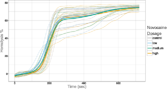
Figure 1: Twenty hemolysis curves (erythrograms) of mice erythrocytes by hydrochloric acid with superimposed estimated mean functions.

Most current approaches essentially evaluate differences among groups of curves point-wise. These approaches treat data that are inherently functional (e.g., hemolysis is a smooth function of time) as a finite vector of observations over time. A typical point-wise approach is to perform a one-way analysis of variance (ANOVA) test at each time point. However, when testing is performed at a large number of points simultaneously, the type I error rate is going to be inflated. Cox and Lee (2008) carefully investigated this issue and proposed a method that utilizes a point-wise ANOVA approach, while properly controlling the type I error rate.

Alternatively, function-valued methods can be employed. A key advantage of the functional approach over its close counterpart—the multivariate approach—is that the former retains information of the ordering and spacing of observations over time. By assuming that there is a true underlying functional response for each subject, function-valued methods explicitly incorporate information over time. Thus, a method is “functional” if it approximates a finite vector of observations by a function (a nonparametric function is a typical choice) and then builds a test statistic based on these functional estimates.

The functional analysis of variance (FANOVA) can be employed to perform testing among $k$ groups of curves. The overall functional testing methods, such as the functional $\mathcal{F}$ of Shen and Faraway (2004) or the functional $V_{n}$ of Cuevas, Febrero and Fraiman (2004), can be utilized to test for associated evidence across the entire functional domain (across all time). Vsevolozhskaya et al. (2013) developed a method for inferences in a FANOVA situation on subregions of the initial functional domain. However, none of these methods [including the point-wise method of Cox and Lee (2008)] allows for pairwise comparisons of functional means. Thus, the challenge for the current analysis was to determine differences among novocaine dosages within specific intervals of time, where significant differences among hemolysis curves are present [these time intervals can be identified based on the methods in Vsevolozhskaya et al. (2013)].

In this paper, we introduce a new function-valued two-step procedure: first, to detect regions in time of significant differences among mean curves, and, second, to perform a pairwise comparison of treatment levels within those regions. The approach utilizes two ideas: (i) combining methods to map a test statistic of the individual hypotheses, $H_{1},\ldots,H_{m}$, to the global one, $\bigcap_{i=1}^{m}H_{i}$, and (ii) the closure principle of Marcus, Peritz and Gabriel (1976) to control the family-wise error rate (FWER), the probability of at least one false rejection. The rest of the article is organized in the following manner. We give an overview of the FANOVA problem and the existing methods for investigating the functional domain for regions where significant differences occur. We discuss the proposed procedure for investigating regions of time for significant differences and detail a computational shortcut that allows isolation of individual significance even for a large number of tests. We extend the proposed procedure to perform pairwise comparisons of the treatment levels within identified functional regions of statistical significance. The protective effect of novocaine is demonstrated based on the different patterns between groups detected in certain regions of time.

2 Methods

Functional analysis of variance involves testing for some difference among $k$ functional means. In functional data analysis, $t$ is used to denote a real-valued variable (usually of time) and $y(t)$ denotes a continuous outcome, which is a function of $t$. Then, the FANOVA model is written as

$$y_{ij}(t)=\mu_{i}(t)+\varepsilon_{ij}(t),$$ (1)

where $\mu_{i}(t)$ is the mean function of group $i$ at time $t$, $i=1,\ldots,k$, $j$ indexes a functional response within a group, $j=1,\ldots,n_{i}$, and $\varepsilon_{ij}(t)$ is the residual function. Each $\varepsilon_{ij}(t)$ is assumed to be a mean zero and independent Gaussian stochastic process. The FANOVA hypotheses are written as

$$H_{0}\dvtx\quad\mu_{1}(t)=\mu_{2}(t)=\cdots=\mu_{k}(t),$$

$$H_{a}\dvtx\quad\mu_{i}(t)\neq\mu_{i^{\prime}}(t)\qquad\mbox{for at least one $t$ and }i\neq i^{\prime}.$$

The alternative hypothesis considers any difference anywhere in $t$ among $k$ population means of $y_{ij}(t)$.

In recent years two different general approaches have emerged to perform the FANOVA test. In Shen and Faraway (2004), as well as many other papers [see Cuevas, Febrero and Fraiman (2004), Ramsay, Hooker and Graves (2009) and Cuesta-Albertos and Febrero-Bande (2010)], a global test statistic has been developed to perform the FANOVA test. The statistic is “global” because it is used to detect differences anywhere in the entire functional domain (anywhere in $t$). An alternative approach [Ramsay and Silverman (2005) and Cox and Lee (2008)] is to use a point-wise (or individual) test statistic to perform inference across $t$, that is, identify specific regions of $t$ with significant difference among functional means.

2.1 “Global” approach

Suppose the domain $[a,b]$ of functional responses can be split into $m$ prespecified mutually exclusive and exhaustive intervals such that $[a,b]=\bigcup_{i=1}^{m}[a_{i},b_{i}]$. For instance, in the novocaine experiment the researchers were interested in the effect of novocaine during specific time intervals associated with hemolysis of different erythrocyte populations: hemolysis of the least stable population ($[a_{2},b_{2}]=61\mbox{--}165$ sec), general population ($[a_{3},b_{3}]=166\mbox{--}240$ sec), and most stable ($[a_{4},b_{4}]={}$over 240 sec). For each interval $[a_{i},b_{i}]$, $i=1,\ldots,m$, an individual functional statistic of Shen and Faraway (2004), $\mathcal{F}_{i},i=1,\ldots,m$, can be calculated as

$$\mathcal{F}_{i}=\frac{\int_{[a_{i},b_{i}]}\sum_{j=1}^{k}n_{j}(\hat{\mu}_{j}(t)-\hat{\mu}(t))^{2}\,dt/(k-1)}{\int_{[a_{i},b_{i}]}\sum_{j=1}^{k}\sum_{s=1}^{n}(y_{js}(t)-\hat{\mu}_{j}(t))^{2}\,dt/(n-k)},$$ (2)

where $n$ is the total number of functional responses and $k$ is the number of groups. The numerator of the $\mathcal{F}$ statistic accounts for “external” variability among functional responses and the denominator for the “internal” variability. Cuevas, Febrero and Fraiman (2004) argue that the null hypothesis should be rejected based on the measure of the differences among groups, that is, the “external” variability. Hence, Cuevas, Febrero and Fraiman (2004) proposed a statistic $V_{n}$ based on the numerator of $\mathcal{F}$:

$$V_{n}=\sum_{i<j}^{k}n_{i}\bigl{\|}\hat{\mu}_{i}(t)-\hat{\mu}_{j}(t)\bigr{\|}^{2},$$ (3)

where $\|\cdot\|$ is the $L_{2}$ norm calculated over the $[a_{i},b_{i}]$ interval. Gower and Krzanowski (1999) also argue that in a permutation setting a test can be based just on the numerator of the test statistic. That is, if only the numerator of the functional $\mathcal{F}$ is used, the changes to the test statistic are monotonic across all permutations and, thus, probabilities obtained are identical to the ones obtained from the original $\mathcal{F}$. Delicado (2007) points out that for a balanced design, the numerator of the functional $\mathcal{F}$ and $V_{n}$ differ by only a multiplicative constant, reinforcing how they provide the same results in a permutation setting. Vsevolozhskaya et al. (2013) fully extended this testing approach by allowing identification of the time interval, $[a_{i},b_{i}]$, $i=1,\ldots,m$, within the time domain, $[a,b]$, while having proper control of at least one false rejection.

2.2 Point-wise approach

Suppose that a set of smooth functional responses is evaluated on a dense grid of points, $t_{1},\ldots,t_{m}$. For instance, the percentage of hemolyzed cells can be evaluated every second. Cox and Lee (2008) propose a test for differences in the mean curves from several populations, that is, perform functional analysis of variance, based on these discretized functional responses. First, at each of the $m$ evaluation points, the regular one-way analysis of variance test statistic, $F_{i},i=1,\ldots,m$, is computed. For each test the $p$-value is calculated based on the parametric $F$-distribution and then the Westfall–Young randomization method [Westfall and Young (1993)] is applied to correct the $p$-values for multiplicity. The implementation of the method can be found in the multtest [Pollard et al. (2011)] R package [R Development Core Team (2012)].

Certain criticisms may be raised for both the “global” and the point-wise approaches. First, the point-wise approach can determine regions of the functional domain with a difference in the means, but there is no clear way to extend this approach to determine which pairs of populations are different. Second, for the Cox and Lee (2008) procedure, the $p$-value for the global test cannot be obtained, which is an undesirable property since the method might be incoherent between the global and point-wise inference. The global approach does not provide the time-specific detail that the point-wise methods provide and the subregion inferences in Vsevolozhskaya et al. (2013) require specification of the subregions which may be arbitrarily defined in some applications. We suggest a procedure that overcomes the majority of these issues. By using a combining function along with the closure principle of Marcus, Peritz and Gabriel (1976), we are able to obtain the $p$-value for the overall test as well as adjust the individual $p$-values for multiplicity. Additionally, the proposed procedure allows us to perform a pairwise comparison of the group’s functional means and therefore determine which populations show evidence of differences in each time region. However, the proposed procedure still requires prespecification of these time regions, which in some applications can be vague.

2.3 Proposed methodology

Once again, suppose the domain $[a,b]$ is split into $m$ prespecified mutually exclusive and exhaustive intervals. We propose to use the numerator of the functional $\mathcal{F}$ as the test statistic $T_{i}$, $i=1,\ldots,m$, for each $[a_{i},b_{i}]$, and then utilize a combining function to obtain the test statistic for the entire $[a,b]$. Typical combining functions have the same general form: the global statistic is defined as a weighted sum, $T=\sum w_{i}T_{i}$, of the individual statistics with some $w_{i}$ weights [see Pesarin (1992) and Basso et al. (2009)]. A $p$-value for the overall null hypothesis (that all individual null hypotheses are true) is based either on the distribution of the resulting global statistic $T$ or on a permutation approximation. If the unweighted sum combining function is applied to the proposed $T_{i}$, then

$$T = \int_{[a,b]}\sum_{j=1}^{k}n_{j}\bigl{(}\hat{\mu}_{j}(t)-\hat{\mu}(t)\bigr{)}^{2}\,dt/(k-1)$$

$$= \sum_{i=1}^{m}\int_{[a_{i},b_{i}]}\sum_{j=1}^{k}n_{j}\bigl{(}\hat{\mu}_{j}(t)-\hat{\mu}(t)\bigr{)}^{2}\,dt/(k-1)$$

$$= \sum_{i=1}^{m}T_{i}.$$

The closure procedure is then applied to perform the overall test based on these combining functions as well as to adjust the individual $p$-values for multiplicity. The closure method is based on testing all nonempty intersections of the set of $m$ individual hypotheses, which together form a closure set. The procedure rejects a given hypothesis if all intersections of hypotheses that contain it as a component are rejected. Hochberg and Tamhane (1987) show that the closure procedure controls the family-wise error rate (FWER) at a strong level, meaning that the type I error is controlled under any partial configuration of true and false null hypotheses.

When the number of individual tests $m$ is relatively large, the use of the closure method becomes computationally challenging. For example, setting $m=15$ results in $2^{15}-1=32\mbox{,}767$ intersections of hypotheses. Hochberg and Tamhane (1987) described a shortcut for the $T=\max\{T_{i}\}$ combining function, where $T_{i}$ stands for the $i$th test statistic for $i$ in the set of $H_{i}$ pertinent to a particular intersection hypothesis. For this combining function they showed that the significance for any given hypothesis in the closure set can be determined using only $m$ individual tests. Zaykin et al. (2002) described a shortcut for the closure principle in the application of their truncated $p$-value method (TPM) that uses an unweighted sum combining function. In the next section we exploit the shortcut described by Zaykin et al. (2002) and show that for the $T=\sum T_{i}$ combining function the required number of evaluations is $m(m+1)/2$.

2.3.1 The shortcut version of the closure procedure

The shortcut version of the closure method for the unweighted sum combining function should be implemented as follows. First, order the individual test statistics from minimum to maximum as $T_{(1)}\leq T_{(2)}\leq\cdots\leq T_{(m)}$, where

$$T_{i}=\int_{[a_{i},b_{i}]}\sum_{j=1}^{k}n_{j}\bigl{(}\hat{\mu}_{j}(t)-\hat{\mu}(t)\bigr{)}^{2}\,dt/(k-1).$$ (4)

Let $H_{(1)},H_{(2)},\ldots,H_{(m)}$ be the corresponding ordered individual hypotheses of no difference among functional means on the interval $[a_{(i)},b_{(i)}]$, $i=1,\ldots,m$. Now, among intersection hypotheses of size two,

$$T_{(1)}+T_{(2)}\leq T_{(1)}+T_{(3)}\leq\cdots\leq T_{(1)}+T_{(m)},$$

$$T_{(2)}+T_{(3)}\leq T_{(2)}+T_{(4)}\leq\cdots\leq T_{(2)}+T_{(m)},$$

$$\cdots$$

Here, the statistic $T_{(i)}+T_{(j)}$ corresponds to intersection hypotheses $H_{(ij)}$ of no significant difference on both intervals $[a_{(i)},b_{(i)}]\cup[a_{(j)},b_{(j)}]$. Among intersections of size three,

$$T_{(1)}+T_{(2)}+T_{(3)}\leq T_{(1)}+T_{(2)}+T_{(4)}\leq\cdots\leq T_{(1)}+T_{(2)}+T_{(m)},$$

$$T_{(2)}+T_{(3)}+T_{(4)}\leq T_{(2)}+T_{(3)}+T_{(5)}\leq\cdots\leq T_{(2)}+T_{(3)}+T_{(m)},$$

$$\cdots$$

Thus, significance for the hypothesis $H_{(m)}$ can be determined by looking for the largest $p$-value among $m$ tests,

$$T_{(m)},T_{(m)}+T_{(1)},\ldots,\sum_{i=1}^{m}T_{(i)}.$$

For the hypothesis $H_{(m-1)}$, the significance can be determined by investigating the $p$-values corresponding to $(m-1)$ tests

$$T_{(m-1)},T_{(m-1)}+T_{(1)},\ldots,\sum_{i=1}^{m-1}T_{(i)},$$

along with the $p$-value for the test $\sum_{i=1}^{m}T_{(i)}$ which is already found. Finally, for the first ordered hypothesis $H_{(1)}$, the significance can be determined by evaluating a single test $T_{(1)}$ and then looking for the largest $p$-value among it and the $p$-values of the hypotheses $H_{(12)}$, $H_{(123)},\ldots,H_{(12\cdots m)}$, which are already evaluated. Thus, significance of any individual hypothesis $H_{(i)}$ is determined using $m$ $p$-values, but the number of unique evaluations to consider is $m+(m-1)+\cdots+1=m(m+1)/2$.

The described shortcut assumes that all distributions corresponding to the test statistics are the same and the magnitude of the test statistic has a monotonic relationship with its $p$-value. If the $p$-values for the individual tests are determined from permutational distributions (as in our situation), a bias will be introduced. The bias is caused by a mismatch between the minimum value of the test statistics and the maximum $p$-value. That is, the minimum statistic is not guaranteed to correspond to the maximum $p$-value. The procedure becomes liberal since the individual $p$-values are not always adjusted adequately. To reduce and possibly eliminate the bias, we made the following adjustment to the shortcut. First, we adjusted the individual $p$-values according to the shortcut protocol described above and obtained a set of adjusted individual $p$-values, $p_{1},p_{2},\ldots,p_{m}$. Then, we ordered the individual test statistics based on the ordering of the unadjusted individual $p$-values. That is, we order the unadjusted $p$-values from maximum to minimum and get a corresponding ordering of the test statistics $T_{(1)}^{*},T_{(2)}^{*},\ldots,T_{(m)}^{*}$. Now the inequality $T^{*}_{(1)}\leq T_{(2)}^{*}\leq\cdots\leq T_{(m)}^{*}$ will not necessarily hold. We applied the shortcut based on this new ordering and obtained another set of adjusted individual $p$-values, $p_{1}^{*},p_{2}^{*},\ldots,p_{m}^{*}$. Finally, the adjusted individual $p$-values were computed as $\max\{p_{i},p_{i}^{*}\},i=1,\ldots,m$. This correction to the shortcut increases the number of the required computations by a factor of two but still is of the order $m^{2}$ instead of $2^{m}$.

A small simulation study was used to check whether this version of the correction provides results comparable to adjustments generated by the entire set of intersection hypotheses. For the four multiplicity adjustment schemes: (i) correction based on the ordered test statistics shortcut, (ii) correction based on the ordered unadjusted $p$-values shortcut, (iii) correction based on $\max\{p_{i},p_{i}^{*}\}$ [combination of both corrections (i) and (ii)], and (iv) the full closure method, we obtained $p$-values under the global null based on 1000 permutations, $m=5$, and conducted 1000 simulations, providing 5000 corrected $p$-values. First, we were interested in how many times the $p$-values adjusted by various shortcuts were “underestimated” (not corrected enough) relative to the full closure method. The $p$-values adjusted by a shortcut based on the ordered test statistics, $p_{1},p_{2},\ldots,p_{m}$, were underestimated 554 out of 5000 times. The $p$-values adjusted by a shortcut based on the ordered unadjusted $p$-values, $p^{*}_{1},p^{*}_{2},\ldots,p^{*}_{m}$, were underestimated 60 out of 5000 times. The $p$-values adjusted using both corrections, $\max\{p_{i},p^{*}_{i}\}$, $i=1,\ldots,m$, were underestimated 38 out of 5000 times. Second, we compared type I error rates under the $\max\{p_{i},p^{*}_{i}\}$ shortcut and the full closure method and found that they were exactly the same. The above results allowed us to conclude that the multiplicity adjustment based on the $\max\{p_{i},p^{*}_{i}\}$ shortcut is adequate.

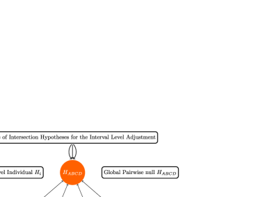
Figure 2: Example of the closure set for the pairwise comparison of four groups.

2.3.2 Proposed methodology for pairwise comparison of functional means

Above, we provided details on how to implement the proposed methodology to isolate regions of the functional domain with statistically significant differences and showed that with a computational shortcut the closed testing scheme is computable even for a large number of individual tests $m$. Now, we show how to further use the proposed methodology to find pairs of functional means that are different within the regions where statistical significance was identified. The procedure is implemented as follows: [(iii)]

Within an interval $[a_{i},b_{i}]$ with a statistically significant difference among functional means, set the $p$-value for the “global” null of no difference among functional means to the adjusted individual $p$-value corresponding to that interval.

Compute the pairwise statistic as well as statistics for the intersection hypotheses as in (4).

Find the $p$-values based on the permutation algorithm and adjust them using the closure principle. Figure 2 illustrates the closure set for pairwise comparison of four populations. The $p$-value of the top node hypothesis, $H_{ABCD}$, of no significant difference among the four population means would be set equal to the adjusted $p$-value of the interval level individual hypothesis of interest $H_{i}$, $i=1,\ldots,m$. The bottom node individual hypotheses, $H_{AB},\ldots,H_{CD}$, correspond to no significant pairwise difference between groups $AB$, $AC,\ldots,CD$ in this interval. Note that now the indexing of the hypotheses corresponds to population means instead of intervals in the functional domain. The closure principle is used to adjust the individual $p$-values.

Certain issues may arise with a test of pairwise comparisons conducted by global randomization. Petrondas and Gabriel (1983) noted that for the overall equality hypothesis all permutations are assumed to be equally probable, that is, the exchangeability among all treatment groups is assumed. However, for the hypothesis of equality of a particular subset of treatments, the global permutation distribution cannot be used because differences in variability among the treatment groups can cause bias in the statistical tests. The results of the simulation study, presented in the next section, did not reveal any noticeable bias in the permutation test. In the case of the pairwise comparison, our method maintained good control of the type I error rate as well as had enough power to correctly identify groups of unequal treatments. The minimal bias observed might be due to a relatively small (three) number of treatments that we chose to consider in our simulation study. Petrondas and Gabriel (1983) and Troendle and Westfall (2011) provide ways to perform permutation tests correctly in the case of the pairwise comparison. We leave implementation of these solutions for future research.

3 Simulations

Before proceeding to the description of our simulation study, we would like to note that all functional data methods, including the one proposed in this article, are affected by how well the estimated functions approximate data. A failure to adequately approximate data with smooth functions may result in a loss of statistical power. An “adequate” approximation is a subjective decision, however, below we outline some choices that are intended to aid fitting particular data at hand.

3.1 Estimation of functional responses

Use of functional data methods requires a “guess” of a function, $\mu(t)$, underlying each response. Since this function is generally unknown, nonparametric methods are used to approximate it. Nonparametric methods represent a function as a linear combination of $K$ “basis functions.” A potential shortcoming of all testing procedures based on nonparametric methods is ambiguity in the choice of basis functions (e.g., splines, Fourier series, Legendre polynomials, etc.) and the number of basis functions, $K$. An incautious choice might lead to over- or under-fit and the resulting loss of statistical power.

The current consensus regarding the choice of basis functions, supported, among others, by Horváth and Kokoszka (2012), Storey et al. (2005), Ramsay and Silverman (2005), is that a good choice should mimic the general features of the data. Specifically, the Fourier basis is recommended for periodic, or nearly periodic, data and the $B$-spline basis for nonperiodic locally smooth data. Since it is known that hemolytic responses have a smooth “S” shape, the $B$-spline basis was a natural choice in our application.

Rice and Wu (2001) and Griswold, Gomulkiewicz and Heckman (2008) investigated the impact of the number of basis functions, $K$, on the quality of fit to the data. More specifically, Rice and Wu (2001) showed that the result of a functional fit is rather insensitive to the specification of the number of basis functions for the $B$-spline basis. Griswold, Gomulkiewicz and Heckman (2008) provided general recommendations for the number of basis functions with an arbitrary basis. They showed that if the data result from (i) an erratically changing stochastic process or (ii) a smoothly varying process with a small measurement error, the recommended number of basis terms required to fit the data is close to the number of observations per subject. We chose the number of basis functions to be close to the number of observations which coincides with the recommendations provided by Griswold, Gomulkiewicz and Heckman (2008). During the course of the novocaine experiment the percent of hemolysis was obtained by converting the spectrophotometric readings. These readings—the measurements of the spectral transmittance—were made with a spectrophotometer PE-5400 VI, which has a low measurement error of $\pm 0.5\%$ (details of the registration certificate are at http://www.promecolab.ru/images/stories/Spektr/5400b-5400UF.pdf). Thus, we had an underlying process that is smooth with a small measurement error so a higher number of basis functions was an appropriate choice.

3.2 Simulations setup

Now, we describe a simulation study that we carried out in order to evaluate the performance of our approach. A nonparametric fit to the data was achieved by employing the $B$-spline basis functions with a “knot” at each observation over $t$. The number of basis functions, $K$, is equal to the number of knots plus two. The simulations scenarios were inspired by a Monte Carlo study in Cuesta-Albertos and Febrero-Bande (2010). We considered [(M1)]

$f_{i}(t)=30(1-t)t-3\beta|\sin(16\pi t)|I_{\{0.325<t<0.3575\}}+\varepsilon_{i}(t)$,

$f_{i}(t)=30(1-t)t-\beta|\sin(\pi t/4)|+\varepsilon_{i}(t)$, where $t_{1}=0,\ldots,t_{101}=1$, $\beta\in\{0.000,0.045,0.091,0.136,0.182,0.227,0.273,\break 0.318,0.364,0.409,0.455,0.500\}$, and random errors $\varepsilon_{i}(t)$ are independently normally distributed with mean zero and variance 0.3. Case M1 (illustrated in Figure 3) corresponds to a situation where a small set of observations was generated under $H_{A}$ to create a spike. In M2 (illustrated in Figure 4), a large number of observations were generated under $H_{A}$ but the differences are less apparent [a deviation along the entire range of $t$ that gradually increases from $\min(t)$ to $\max(t)$]. The parameter $\beta$ controls the strength of the deviation from the global null. The reason for considering these two cases was to check the performance of our method for different ranges of false null hypotheses.

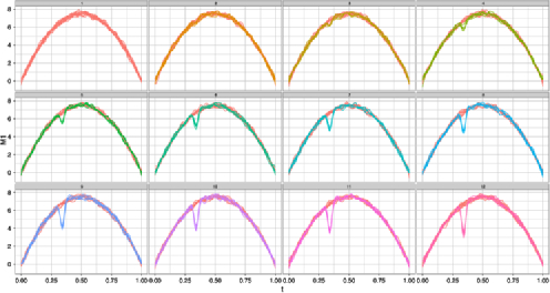
Figure 3: Plot of the data for one simulation replicate under the M1 case and 12 different values of $\beta$. The functions that have the mean value, $\mu_{3}(t)$, deviating from the overall mean ($\mu_{1}(t)=\mu_{2}(t)\equiv\mu(t)$) are highlighted in a color.

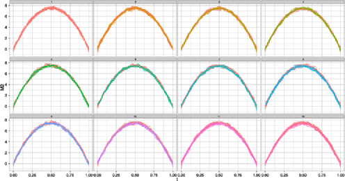
Figure 4: Plot of the data for one simulation replicate under the M2 case and 12 different values of $\beta$. The functions that have the mean value deviating from the overall mean are highlighted in a color.

In each case (M1 and M2), we generated three samples of functional data with 5 observations from each group. The first two samples had the same mean ($\beta=0$) and the third sample’s mean was deviating ($\beta\neq 0$). Once the functional data were generated for different values of $\beta\neq 0$, we split the functional domain into different numbers of equal-length intervals ($m=5$ and $m=10$) and evaluated the power of rejecting the null hypotheses $H_{0}\dvtx\mu_{1}(t)=\mu_{2}(t)=\mu_{3}(t)$ at the 5% level. We used 1000 simulations to obtain a set of power values for each combination of $\beta$ and $m$ values. We used a permutation test to obtain the $p$-values. This was achieved by randomly permuting the original observations for each $t$ across groups 1000 times, and for each new grouping, refitting the functional means and recalculating the value of the test statistic. The $p$-value was found as the proportion of 1000 recalculated test statistics greater than the observed statistic.

3.3 Simulation results

Figure 5 presents results of power evaluation for model M1 and five intervals ($m=5$). Under this model, a set of observations generated under $H_{A}$ fell into the second interval. That is, the functional mean of the third sample had a spike deviation from the functional mean of the first two samples over the second interval. The magnitude of the spike increased monotonically as a function of $\beta$. The plot shows that the proportion of rejections reveals a peak over the region of the true deviation, while being conservative over the locations with no deviations. Thus, we conclude that the proposed methodology provides satisfactory power over the region with true differences, while being conservative over the regions where the null hypothesis is true.

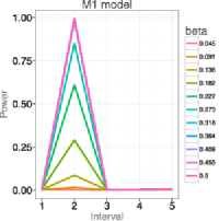
Figure 5: The probability of rejecting the null hypothesis $H_{0}\dvtx\mu_{1}(t)=\mu_{2}(t)=\mu_{3}(t)$ for $m=5$ intervals.

Once we identified the region of the functional domain with differences in means (i.e., the second interval), we used the extension of the proposed methodology to perform a pairwise comparison and determine which populations are different. Figure 6 provides the results of power evaluation of the pairwise comparisons at the 5% significance level. In the case of $H_{AB}$ (where the null $\mu_{1}=\mu_{2}$ is true), the simulation output tells us that the procedure is a bit conservative, maintaining the type I error rate right below the 5% level for the higher values of $\beta$. In the case of $H_{AC}$ and $H_{BC}$ (where the null is false), it can be seen that the power of the pairwise comparison is satisfactory.

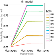
Figure 6: The probability of rejecting individual pairwise hypotheses $H_{AB}\dvtx\mu_{1}(t)=\mu_{2}(t)$, $H_{AC}\dvtx\mu_{1}(t)=\mu_{3}(t)$, and $H_{BC}\dvtx\mu_{2}(t)=\mu_{3}(t)$.

Table 1: Power of the pairwise comparison assuming common means $\mu_{1}$ and $\mu_{2}$ over the 1st interval

$\bolds{\beta}$	$\bolds{H_{AB}\dvtx\mu_{1}=\mu_{2}}$	$\bolds{H_{AC}\dvtx\mu_{1}=\mu_{3}}$	$\bolds{H_{BC}\dvtx\mu_{2}=\mu_{3}}$
0.318	0.027	0.021	0.026
0.364	0.029	0.024	0.028
0.409	0.031	0.034	0.038
0.455	0.036	0.041	0.047
0.500	0.036	0.049	0.054

Table 2: Power of the pairwise comparison assuming common means $\mu_{1}$ and $\mu_{2}$ over the 2nd interval

$\bolds{\beta}$	$\bolds{H_{AB}\dvtx\mu_{1}=\mu_{2}}$	$\bolds{H_{AC}\dvtx\mu_{1}=\mu_{3}}$	$\bolds{H_{BC}\dvtx\mu_{2}=\mu_{3}}$
0.273	0.018	0.049	0.057
0.318	0.025	0.074	0.086
0.364	0.031	0.104	0.116
0.409	0.037	0.145	0.164
0.455	0.041	0.214	0.224
0.500	0.045	0.298	0.323

The results for the M2 case, where the number of true effects is large and the magnitude of the effect gradually increases from $\min(t)$ to $\max(t)$, are provided in Tables 1–5 and Figure 7. The plot shows that for a fixed value $\beta$, the proportion of rejections of the hypothesis $H_{0}\dvtx\mu_{1}(t)=\mu_{2}(t)=\mu_{3}(t)$ gradually increases with the magnitude of the effect. Across different values of $\beta$, power values are also increasing, attaining the value of 1 for the fifth interval and $\beta=0.5$. The results of the pairwise comparisons are provided in Tables 1–5. Power is the highest for the highest value of $\beta$ (0.5), but overall the method does a good job of picking out the differences between $\mu_{1}$ and $\mu_{3}$, and $\mu_{2}$ and $\mu_{3}$, while maintaining control of spurious rejections for $\mu_{1}$ and $\mu_{2}$.

Table 3: Power of the pairwise comparison assuming common means $\mu_{1}$ and $\mu_{2}$ over the 3rd interval

$\bolds{\beta}$	$\bolds{H_{AB}\dvtx\mu_{1}=\mu_{2}}$	$\bolds{H_{AC}\dvtx\mu_{1}=\mu_{3}}$	$\bolds{H_{BC}\dvtx\mu_{2}=\mu_{3}}$
0.182	0.015	0.038	0.040
0.227	0.021	0.077	0.084
0.273	0.027	0.160	0.155
0.318	0.037	0.289	0.275
0.364	0.041	0.437	0.434
0.409	0.048	0.610	0.600
0.455	0.048	0.731	0.735
0.500	0.049	0.839	0.835

Table 4: Power of the pairwise comparison assuming common means $\mu_{1}$ and $\mu_{2}$ over the 4th interval

$\bolds{\beta}$	$\bolds{H_{AB}\dvtx\mu_{1}=\mu_{2}}$	$\bolds{H_{AC}\dvtx\mu_{1}=\mu_{3}}$	$\bolds{H_{BC}\dvtx\mu_{2}=\mu_{3}}$
0.182	0.017	0.082	0.080
0.227	0.023	0.207	0.196
0.273	0.030	0.375	0.365
0.318	0.036	0.618	0.611
0.364	0.039	0.817	0.807
0.409	0.041	0.920	0.915
0.455	0.041	0.971	0.971
0.500	0.041	0.993	0.993

Table 5: Power of the pairwise comparison assuming common means $\mu_{1}$ and $\mu_{2}$ over the 5th interval

$\bolds{\beta}$	$\bolds{H_{AB}\dvtx\mu_{1}=\mu_{2}}$	$\bolds{H_{AC}\dvtx\mu_{1}=\mu_{3}}$	$\bolds{H_{BC}\dvtx\mu_{2}=\mu_{3}}$
0.136	0.012	0.044	0.042
0.182	0.020	0.164	0.160
0.227	0.030	0.380	0.383
0.273	0.038	0.640	0.645
0.318	0.041	0.858	0.859
0.364	0.042	0.955	0.957
0.409	0.042	0.986	0.988
0.455	0.042	0.997	1.000
0.500	0.042	1.000	1.000

Results based on $m=10$ intervals are similar to those based on $m=5$ intervals and can be found in the supplementary material [Vsevolozhskaya, Greenwood and Holodov (2014)]. A careful consideration of these results, however, reveals that the procedure tends to lose power as the number of intervals increases but gains power as the number of curves per group increases.

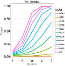
Figure 7: The probability of rejecting the null hypothesis $H_{0}\dvtx\mu_{1}(t)=\mu_{2}(t)=\mu_{3}(t)$ in the case of the M2 model and 5 intervals.

4 Analysis of hemolysis curves

In this section we illustrate the proposed methodology by applying it to a study of the effect of novocaine conducted by Holodov and Nikolaevski (2012). The motivation behind the study was to investigate pharmaceutical means of preventing the formation of stomach erosive and ulcerative lesions caused by a long-term use of nonsteroidal anti-inflammatory drugs (NSAIDs). Internal use of a novocaine solution was proposed as a preventative treatment for NSAID-dependent complications.

During the course of the experiment, blood was drawn from male rats to obtain an erythrocyte suspension. Then, four different treatments were applied: control, low ($4.9\times 10^{-6}$ mol/L), medium ($1.0\times 10^{-5}$ mol/L), and high ($2.01\times 10^{-5}$ mol/L) dosages of procaine. After treatment application, the erythrocyte suspension was incubated for 0, 15, 30, 60, 120 or 240 minutes. At the end of each incubation period, hemolysis was initiated by adding 0.1 M of hydrochloric acid to the erythrocyte suspension. The percent of hemolysis or the percent of red blood cells that had broken down was measured every 15 seconds for 12 minutes. The experiment was repeated 5 times for each dosage/incubation combination using different rats. Therefore, the data set consists of 120 separate runs with 49 discretized observations per run and involves four experimental conditions with six incubation times, replicated 5 times for each treatment/incubation combination. For more details see Holodov and Nikolaevski (2012).

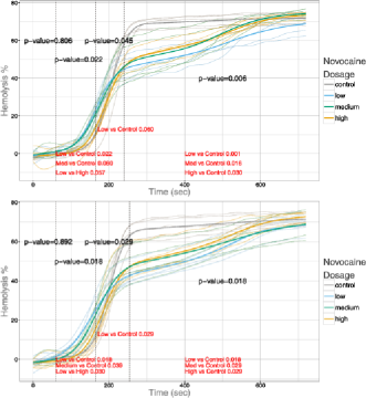
Figure 8: Erythrogram means for the control group and the treatment groups for 15 (top graph) and 30 (bottom graph) minute incubation times.

We fit the data with smoothing cubic $B$-splines with 49 equally spaced knots at times $t_{1}=0,\ldots,t_{49}=720$ seconds to generate the functional data. The reasoning behind these choices is provided in Section 3.1. A smoothing parameter was selected by generalized cross-validation (GCV) for each functional observation with an increased penalty for each effective degree of freedom in the GCV, as recommended in Wood (2006).

To keep the analysis as simple as possible, each incubation data set was analyzed for treatment effects separately. Our initial test was to check for a significant difference in mean erythrograms (mean hemolysis curves) anywhere in time among novocaine dosages. A Bonferroni correction was applied to these initial $p$-values to adjust for multiplicity at this level. The results indicated strong evidence of differences for the 15 and 30 minute incubation times ($p$-value${}_{\mathrm{Bonf}}=0.006$ and $p$-value${}_{\mathrm{Bonf}}=0.018$, resp.). Figure 8 illustrates the results for these incubation times. For the rest of the incubation times, we found no evidence against the null hypothesis that the four erythrogram means coincided, so no further analysis was conducted.

Next, we examined the 15 and 30 minute incubation results in more detail to asses the nature of the differences. For both incubation times, four time intervals of interest were prespecified: (i) the latent period (0–60 sec), (ii) hemolysis of the population of the least stable red blood cells (61–165 sec), (iii) hemolysis of the general red blood cell population (166–240 sec), and (iv) the plateau (over 240 sec). The latent period is associated with erythrocytes spherulation and occurs between addition of the hemolytic agent and initiation of hemolysis. The names of the next two periods are self-explanatory. The plateau period is associated with deterioration of the population of the most stable erythrocytes.

We applied our method to determine if statistical significance is present in each of the four time intervals. In the application of our method, we set the $p$-values for the global hypotheses $H_{1234}$ of no significant difference on all four intervals to the Bonferroni adjusted $p$-values obtained on the previous step. For the 15 minute incubation time, no statistical significance was found during the latent period ($p$-value${}=0.806$), and statistically significant results were found during hemolysis of the least stable red blood cell population ($p$-value${}=0.022$), general red blood cell population (marginal significance with the $p$-value${}=0.060$) and plateau ($p$-value${}=0.006$). The same results were obtained from the 30 minute incubation, that is, no statistical significance during the latent period ($p$-value${}=0.892$) and statistical significance for the rest of the time intervals with $p$-values of 0.018, 0.029 and 0.018 for the periods of hemolysis of the least stable population, general population and plateau, respectively.

Finally, we were interested in pairwise comparison of treatment levels within the time intervals of statistical significance. Once again, similar results were found for both incubation times, although the $p$-values were often larger for the 15 minute incubation time. During the hemolysis of the least stable red blood cell population, at least some evidence was found of a difference between low dosage and control ($p$-value${}_{15}=0.020$, $p$-value${}_{30}=0.018$), medium dosage and control ($p$-value${}_{15}=0.060$, $p$-value${}_{30}=0.039$), and low dosage and high dosage ($p$-value${}_{15}=0.057$, $p$-value${}_{30}=0.030$). During the hemolysis of the general population, at least some evidence of a significant difference was found between the low dose and control ($p$-value${}_{15}=0.060$, $p$-value${}_{30}=0.029$). During the plateau interval, there was a significant difference between low dose and control ($p$-value${}_{15}=0.001$, $p$-value${}_{30}=0.018$), medium dose and control ($p$-value${}_{15}=0.016$, $p$-value${}_{30}=0.029$), and high dose and control ($p$-value${}_{15}=0.030$, $p$-value${}_{30}=0.029$).

The results of the analysis can be summarized as follows. The rate of hemolysis increases with the dosage of novocaine. That is, the structural and functional modifications in the erythrocyte’s membrane induced by novocaine are dosage dependent. The results also indicate the distribution of erythrocytes into subpopulations with low, medium and high resistance to hemolysis. These populations modified by novocaine react differently with the hemolytic agent. After 15 and 30 minutes of incubation, the “old” erythrocytes (least stable) modified by low ($4.9\times 10^{-6}$ mol/L) and medium ($1.0\times 10^{-5}$ mol/L) doses of procaine react faster to the hemolytic agent than those under the control or the high ($2.01\times 10^{-5}$ mol/L) dose. However, reaction of the general and “young” (most stable) erythrocyte population modified by the same (low and medium) dosages is characterized by higher stability of the membrane and thus have higher resistance to the hemolytic agent. Thus, novocaine in low and medium doses has a protective effect on the general and “young” erythrocyte populations. However, an increase in procaine dosage does not lead to an increase of erythrocyte resistance to the hemolytic agent. The effect of the high dose of novocaine ($2.01\times 10^{-5}$ mol/L) does not differ significantly from the control and thus is destructive rather than protective.

Conclusions of our statistical analysis confirm certain findings reported in a patent by Holodov and Nikolaevski (2012). Specifically, our analysis confirms that novocaine in low dosages tends to have a protective effect. However, Holodov and Nikolaevski (2012) reported a significant difference among erythrograms for all incubation times but zero minutes. This inconsistency is due to a failure to properly adjust the number of tests performed in the original analysis. The findings reported in the current paper have a higher assurance that a replication experiment will be able to detect the same differences reported here.

5 Discussion

We have suggested a procedure which allows researchers to find regions of significant difference in the domain of functional responses as well as to determine which populations are different over these regions. To the best of our knowledge, there are no existing competing procedures to the proposed methodology. Thus, our numerical results reported in Section 3 do not include a comparison of the proposed method to other alternatives. Nevertheless, the simulations revealed that our procedure has satisfactory power and does a good job of picking out the differences between population means. Also, in our simulation study, a relatively small number of regions ($m=5$ and $m=10$) were considered. A higher number of individual tests (intervals) can be easily implemented with the described shortcut to the closure principle.

The relative efficiency of all nonparametric functional approaches depends on the “adequate” representation of data by smooth functions. In Section 3.1 we provided some general recommendations that should help a reader to choose an effective basis and a number of basis functions for a particular application. A valid point raised by one of the reviewers was that if power of any function-valued statistical procedure depends on the accuracy of the estimates of individual curves, they, in turn, might depend on the number of observed time points per subject. Griswold, Gomulkiewicz and Heckman (2008) studied this issue and showed that as the number of measurements per subject increased from 10 to 20, the power of a functional approach remained relatively constant or improved. Berk, Ebbels and Montana (2011) used as little as 10 observations per subject to estimate the functional responses. Thus, we expect statistical power to be rather insensitive to the number of time points at hand as long as researchers have at least 10 observations and are producing reasonable functional estimates.

Another important issue is that the nonparametric approaches based on the $B$-spline basis might suffer from a phenomenon termed “edge effect”—a bias in the estimation at the endpoints. Thus, power of the procedure to detect differences among functional responses might be affected at the intervals near the edges if the estimated smooth functions have boundary artifacts (e.g., unexpected behavior). This was not the case in our simulation study nor in our application. If a researcher encounters functional boundary artifacts while fitting particular data of interest, s/he might consider correcting for this effect [e.g., see Masri and Redner (2005)].

We also note that for the procedure presented in this article, the regions of interest in the functional domain should be prespecified prior to the analysis. However, in our experience researchers have never had a problem with a priori region identification. From previous research, expected results as well as specific regions of interest are typically known. We also mention that in the application of our method the intervals should be mutually exclusive and exhaustive. If researchers are interested in a test over overlapping intervals, the solution is to split the functional domain into smaller mutually exclusive intervals for individual tests (terminal nodes of the hypotheses tree). The decision for the overlapping region would be provided by a test of an intersection hypothesis (“higher” node in the hypotheses tree). We also expect the intervals to be exhaustive since it would be unexpected for researchers to collect data over time periods that they have no interest in. Finally, if for some reason distinct regions cannot be prespecified, a large number of equal sized intervals can easily be employed, however, this might result in loss of power.

The present work has two open issues that suggest a direction for future research. First, the method is conservative and so a more powerful approach may be possible. Second, the permutation strategy for the pairwise comparison test may lead to biased inference. Solutions to the latter problem were suggested both by Petrondas and Gabriel (1983) and Troendle and Westfall (2011). We leave implementation of these solutions for future research, as this seems to be a minor issue with a small number of treatment groups as are most often encountered in FANOVA applications.

[id=suppA] Additional simulation results [doi]10.1214/14-AOAS723SUPP .pdf aoas723_supp.pdf Additional simulation results for the two models (M1 or M2), two different number of intervals ($m=5$ or $m=10$), and either 5 or 20 subjects per group are summarized in the tables below. Overall, these results indicate that the procedure tends to lose power as the number of intervals increases but gains power as the number of subjects per group increases.

References

- Basso et al. (2009) {bbook}[auto:STB—2014/02/12—14:17:21] \bauthor\bsnmBasso, \bfnmD.\binitsD., \bauthor\bsnmPesarin, \bfnmF.\binitsF., \bauthor\bsnmSolmaso, \bfnmL.\binitsL. and \bauthor\bsnmSolari, \bfnmA.\binitsA. (\byear2009). \btitlePermutation Tests for Stochastic Ordering and ANOVA: Theory and Applications with R. \bpublisherSpringer,\blocationDordrecht.\bptokimsref\endbibitem
- Berk, Ebbels and Montana (2011) {barticle}[pbm] \bauthor\bsnmBerk, \bfnmMaurice\binitsM., \bauthor\bsnmEbbels, \bfnmTimothy\binitsT. and \bauthor\bsnmMontana, \bfnmGiovanni\binitsG. (\byear2011). \btitleA statistical framework for biomarker discovery in metabolomic time course data. \bjournalBioinformatics \bvolume27 \bpages1979–1985. \biddoi=10.1093/bioinformatics/btr289, issn=1367-4811, pii=btr289, pmcid=3129523, pmid=21729866 \bptokimsref\endbibitem
- Cox and Lee (2008) {barticle}[mr] \bauthor\bsnmCox, \bfnmDennis D.\binitsD. D. and \bauthor\bsnmLee, \bfnmJong Soo\binitsJ. S. (\byear2008). \btitlePointwise testing with functional data using the Westfall–Young randomization method. \bjournalBiometrika \bvolume95 \bpages621–634. \biddoi=10.1093/biomet/asn021, issn=0006-3444, mr=2443179 \bptokimsref\endbibitem
- Cuesta-Albertos and Febrero-Bande (2010) {barticle}[mr] \bauthor\bsnmCuesta-Albertos, \bfnmJ. A.\binitsJ. A. and \bauthor\bsnmFebrero-Bande, \bfnmM.\binitsM. (\byear2010). \btitleA simple multiway ANOVA for functional data. \bjournalTEST \bvolume19 \bpages537–557. \biddoi=10.1007/s11749-010-0185-3, issn=1133-0686, mr=2746001 \bptokimsref\endbibitem
- Cuevas, Febrero and Fraiman (2004) {barticle}[mr] \bauthor\bsnmCuevas, \bfnmAntonio\binitsA., \bauthor\bsnmFebrero, \bfnmManuel\binitsM. and \bauthor\bsnmFraiman, \bfnmRicardo\binitsR. (\byear2004). \btitleAn anova test for functional data. \bjournalComput. Statist. Data Anal. \bvolume47 \bpages111–122. \biddoi=10.1016/j.csda.2003.10.021, issn=0167-9473, mr=2087932 \bptokimsref\endbibitem
- Delicado (2007) {barticle}[mr] \bauthor\bsnmDelicado, \bfnmPedro\binitsP. (\byear2007). \btitleFunctional -sample problem when data are density functions. \bjournalComput. Statist. \bvolume22 \bpages391–410. \biddoi=10.1007/s00180-007-0047-y, issn=0943-4062, mr=2336343 \bptokimsref\endbibitem
- García Rodríguez, Hernández-Díaz and de Abajo (2001) {barticle}[pbm] \bauthor\bsnmGarcía Rodríguez, \bfnmL. A.\binitsL. A., \bauthor\bsnmHernández-Díaz, \bfnmS.\binitsS. and \bauthor\bparticlede \bsnmAbajo, \bfnmF. J.\binitsF. J. (\byear2001). \btitleAssociation between aspirin and upper gastrointestinal complications: Systematic review of epidemiologic studies. \bjournalBr. J. Clin. Pharmacol. \bvolume52 \bpages563–571. \bidissn=0306-5251, pii=1476, pmcid=2014603, pmid=11736865 \bptokimsref\endbibitem
- Gower and Krzanowski (1999) {barticle}[auto:STB—2014/02/12—14:17:21] \bauthor\bsnmGower, \bfnmJ. C.\binitsJ. C. and \bauthor\bsnmKrzanowski, \bfnmW. J.\binitsW. J. (\byear1999). \btitleAnalysis of distance for structured multivariate data and extensions to multivariate analysis of variance. \bjournalJ. R. Stat. Soc. Ser. C. Appl. Stat. \bvolume48 \bpages505–519. \bptokimsref\endbibitem
- Griswold, Gomulkiewicz and Heckman (2008) {barticle}[pbm] \bauthor\bsnmGriswold, \bfnmCortland K.\binitsC. K., \bauthor\bsnmGomulkiewicz, \bfnmRichard\binitsR. and \bauthor\bsnmHeckman, \bfnmNancy\binitsN. (\byear2008). \btitleHypothesis testing in comparative and experimental studies of function-valued traits. \bjournalEvolution \bvolume62 \bpages1229–1242. \biddoi=10.1111/j.1558-5646.2008.00340.x, issn=0014-3820, pii=EVO340, pmid=18266991 \bptokimsref\endbibitem
- Hochberg and Tamhane (1987) {bbook}[mr] \bauthor\bsnmHochberg, \bfnmYosef\binitsY. and \bauthor\bsnmTamhane, \bfnmAjit C.\binitsA. C. (\byear1987). \btitleMultiple Comparison Procedures. \bpublisherWiley, \blocationNew York. \biddoi=10.1002/9780470316672, mr=0914493 \bptokimsref\endbibitem
- Holodov and Nikolaevski (2012) {bmisc}[auto:STB—2014/02/12—14:17:21] \bauthor\bsnmHolodov, \bfnmD. B.\binitsD. B. and \bauthor\bsnmNikolaevski, \bfnmV. A.\binitsV. A. (\byear2012). \bhowpublishedA method for preventing damages to the stomach mucous membrane when taking non-steroidal anti-inflammatory drugs. Patent RU 2449784. Available at http://www.findpatent.ru/patent/244/2449784.html. \bptokimsref\endbibitem
- Horváth and Kokoszka (2012) {bbook}[mr] \bauthor\bsnmHorváth, \bfnmLajos\binitsL. and \bauthor\bsnmKokoszka, \bfnmPiotr\binitsP. (\byear2012). \btitleInference for Functional Data with Applications. \bpublisherSpringer, \blocationNew York. \biddoi=10.1007/978-1-4614-3655-3, mr=2920735 \bptokimsref\endbibitem
- Marcus, Peritz and Gabriel (1976) {barticle}[mr] \bauthor\bsnmMarcus, \bfnmRuth\binitsR., \bauthor\bsnmPeritz, \bfnmEric\binitsE. and \bauthor\bsnmGabriel, \bfnmK. R.\binitsK. R. (\byear1976). \btitleOn closed testing procedures with special reference to ordered analysis of variance. \bjournalBiometrika \bvolume63 \bpages655–660. \bidissn=0006-3444, mr=0468056 \bptokimsref\endbibitem
- Masri and Redner (2005) {barticle}[mr] \bauthor\bsnmMasri, \bfnmRiad\binitsR. and \bauthor\bsnmRedner, \bfnmRichard A.\binitsR. A. (\byear2005). \btitleConvergence rates for uniform -spline density estimators on bounded and semi-infinite domains. \bjournalJ. Nonparametr. Stat. \bvolume17 \bpages555–582. \biddoi=10.1080/10485250500039239, issn=1048-5252, mr=2141362 \bptnotecheck year \bptokimsref\endbibitem
- Nasonov and Karateev (2006) {barticle}[auto:STB—2014/02/12—14:17:21] \bauthor\bsnmNasonov, \bfnmE. L.\binitsE. L. and \bauthor\bsnmKarateev, \bfnmA. E.\binitsA. E. (\byear2006). \btitleThe use of non-steroidal anti-inflammatory drugs: Clinical recommendations. \bjournalRussian Medical Journal \bvolume14 \bpages1769–1777. \bptokimsref\endbibitem
- Pesarin (1992) {barticle}[auto:STB—2014/02/12—14:17:21] \bauthor\bsnmPesarin, \bfnmF.\binitsF. (\byear1992). \btitleA resampling procedure for nonparametric combination of several dependent tests. \bjournalStat. Methods Appl. \bvolume1 \bpages87–101. \bptokimsref\endbibitem
- Petrondas and Gabriel (1983) {barticle}[auto:STB—2014/02/12—14:17:21] \bauthor\bsnmPetrondas, \bfnmD. A.\binitsD. A. and \bauthor\bsnmGabriel, \bfnmK. R.\binitsK. R. (\byear1983). \btitleMultiple comparisons by rerandomization tests. \bjournalJ. Amer. Statist. Assoc. \bvolume78 \bpages949–957. \bptokimsref\endbibitem
- Pollard et al. (2011) {bmisc}[auto:STB—2014/02/12—14:17:21] \bauthor\bsnmPollard, \bfnmK. S.\binitsK. S., \bauthor\bsnmGilbert, \bfnmH. N.\binitsH. N., \bauthor\bsnmGe, \bfnmY.\binitsY., \bauthor\bsnmTaylor, \bfnmS.\binitsS. and \bauthor\bsnmDudoit, \bfnmS.\binitsS. (\byear2011). \bhowpublishedmulttest: Resampling-based multiple hypothesis testing. R package version 2.10.0. \bptokimsref\endbibitem
- R Development Core Team (2012) {bmisc}[auto:STB—2014/02/12—14:17:21] \borganizationR Development Core Team (\byear2012). \bhowpublishedR: A Language and Environment for Statistical Computing. R Foundation for Statistical Computing, Vienna, Austria. ISBN 3-900051-07-0. Available at http://www.R-project.org/. \bptokimsref\endbibitem
- Ramsay, Hooker and Graves (2009) {bbook}[auto:STB—2014/02/12—14:17:21] \bauthor\bsnmRamsay, \bfnmJ. O.\binitsJ. O., \bauthor\bsnmHooker, \bfnmG.\binitsG. and \bauthor\bsnmGraves, \bfnmS.\binitsS. (\byear2009). \btitleFunctional Data Analysis with R and MATLAB. \bpublisherSpringer, \blocationDordrecht. \bptokimsref\endbibitem
- Ramsay and Silverman (2005) {bbook}[mr] \bauthor\bsnmRamsay, \bfnmJ. O.\binitsJ. O. and \bauthor\bsnmSilverman, \bfnmB. W.\binitsB. W. (\byear2005). \btitleFunctional Data Analysis, \bedition2nd ed. \bpublisherSpringer, \blocationNew York. \bidmr=2168993 \bptokimsref\endbibitem
- Rice and Wu (2001) {barticle}[mr] \bauthor\bsnmRice, \bfnmJohn A.\binitsJ. A. and \bauthor\bsnmWu, \bfnmColin O.\binitsC. O. (\byear2001). \btitleNonparametric mixed effects models for unequally sampled noisy curves. \bjournalBiometrics \bvolume57 \bpages253–259. \biddoi=10.1111/j.0006-341X.2001.00253.x, issn=0006-341X, mr=1833314 \bptokimsref\endbibitem
- Shen and Faraway (2004) {barticle}[mr] \bauthor\bsnmShen, \bfnmQing\binitsQ. and \bauthor\bsnmFaraway, \bfnmJulian\binitsJ. (\byear2004). \btitleAn test for linear models with functional responses. \bjournalStatist. Sinica \bvolume14 \bpages1239–1257. \bidissn=1017-0405, mr=2126351 \bptokimsref\endbibitem
- Storey et al. (2005) {barticle}[auto:STB—2014/02/12—14:17:21] \bauthor\bsnmStorey, \bfnmJ. D.\binitsJ. D., \bauthor\bsnmXiao, \bfnmW.\binitsW., \bauthor\bsnmLeek, \bfnmJ. T.\binitsJ. T., \bauthor\bsnmTompkins, \bfnmR. G.\binitsR. G. and \bauthor\bsnmDavis, \bfnmR. D.\binitsR. D. (\byear2005). \btitleSignificance analysis of time course microarray experiments. \bjournalProc. Natl. Acad. Sci. USA \bvolume120 \bpages12837–12842. \bptokimsref\endbibitem
- Troendle and Westfall (2011) {barticle}[mr] \bauthor\bsnmTroendle, \bfnmJames F.\binitsJ. F. and \bauthor\bsnmWestfall, \bfnmPeter H.\binitsP. H. (\byear2011). \btitlePermutational multiple testing adjustments with multivariate multiple group data. \bjournalJ. Statist. Plann. Inference \bvolume141 \bpages2021–2029. \biddoi=10.1016/j.jspi.2010.12.012, issn=0378-3758, mr=2772208 \bptokimsref\endbibitem
- Vsevolozhskaya, Greenwood and Holodov (2014) {bmisc}[auto:STB—2014/02/12—14:17:21] \bauthor\bsnmVsevolozhskaya, \bfnmO. A.\binitsO. A., \bauthor\bsnmGreenwood, \bfnmM. C.\binitsM. C. and \bauthor\bsnmHolodov, \bfnmD.\binitsD. (\byear2014). \bhowpublishedSupplement to “Pairwise comparison of treatment levels in functional analysis of variance with application to erythrocyte hemolysis.” DOI:\doiurl10.1214/14-AOAS723SUPP. \bptokimsref\endbibitem
- Vsevolozhskaya et al. (2013) {barticle}[mr] \bauthor\bsnmVsevolozhskaya, \bfnmO. A.\binitsO. A., \bauthor\bsnmGreenwood, \bfnmM. C.\binitsM. C., \bauthor\bsnmBellante, \bfnmG. J.\binitsG. J., \bauthor\bsnmPowell, \bfnmS. L.\binitsS. L., \bauthor\bsnmLawrence, \bfnmR. L.\binitsR. L. and \bauthor\bsnmRepasky, \bfnmK. S.\binitsK. S. (\byear2013). \btitleCombining functions and the closure principle for performing follow-up tests in functional analysis of variance. \bjournalComput. Statist. Data Anal. \bvolume67 \bpages175–184. \biddoi=10.1016/j.csda.2013.05.005, issn=0167-9473, mr=3079595 \bptokimsref\endbibitem
- Westfall and Young (1993) {bbook}[auto:STB—2014/02/12—14:17:21] \bauthor\bsnmWestfall, \bfnmP. H.\binitsP. H. and \bauthor\bsnmYoung, \bfnmS. S.\binitsS. S. (\byear1993). \btitleResampling-Based Multiple Testing: Examples and Methods for P-Values Adjustment. \bpublisherWiley, \blocationNew York. \bptokimsref\endbibitem
- Wood (2006) {bbook}[mr] \bauthor\bsnmWood, \bfnmSimon N.\binitsS. N. (\byear2006). \btitleGeneralized Additive Models: An Introduction with . \bpublisherChapman & Hall/CRC, \blocationBoca Raton, FL. \bidmr=2206355 \bptokimsref\endbibitem
- Zaykin et al. (2002) {barticle}[pbm] \bauthor\bsnmZaykin, \bfnmD. V.\binitsD. V., \bauthor\bsnmZhivotovsky, \bfnmLev A.\binitsL. A., \bauthor\bsnmWestfall, \bfnmP. H.\binitsP. H. and \bauthor\bsnmWeir, \bfnmB. S.\binitsB. S. (\byear2002). \btitleTruncated product method for combining -values. \bjournalGenet. Epidemiol. \bvolume22 \bpages170–185. \biddoi=10.1002/gepi.0042, issn=0741-0395, pii=10.1002/gepi.0042, pmid=11788962 \bptokimsref\endbibitem