Focusing Quantum Many-body Dynamics II:
The Rigorous Derivation of the 1D Focusing Cubic Nonlinear Schrödinger Equation from 3D

Abstract.

We consider the focusing 3D quantum many-body dynamic which models a dilute bose gas strongly confined in two spatial directions. We assume that the microscopic pair interaction is attractive and given by $a^{3\beta-1}V(a^{\beta}\cdot)$ where $\int V\leqslant 0$ and $a$ matches the Gross-Pitaevskii scaling condition. We carefully examine the effects of the fine interplay between the strength of the confining potential and the number of particles on the 3D $N$-body dynamic. We overcome the difficulties generated by the attractive interaction in 3D and establish new focusing energy estimates. We study the corresponding BBGKY hierarchy which contains a diverging coefficient as the strength of the confining potential tends to $\infty$. We prove that the limiting structure of the density matrices counterbalances this diverging coefficient. We establish the convergence of the BBGKY sequence and hence the propagation of chaos for the focusing quantum many-body system. We derive rigorously the 1D focusing cubic NLS as the mean-field limit of this 3D focusing quantum many-body dynamic and obtain the exact 3D to 1D coupling constant.

1. Introduction

Since the Nobel prize winning first observation of Bose-Einstein condensate (BEC) in 1995 [4, 25], the investigation of this new state of matter has become one of the most active areas of contemporary research. A BEC, first predicted theoretically by Einstein for non-interacting particles in 1925, is a peculiar gaseous state that particles of integer spin (bosons) occupy a macroscopic quantum state.

Let $t\in\mathbb{R}$ be the time variable and $\mathbf{r}_{N}=\left(r_{1},r_{2},...,r_{N}\right)\in\mathbb{R}^{nN}$ be the position vector of $N$ particles in $\mathbb{R}^{n}$, then, naively, BEC means that, up to a phase factor solely depending on $t,$ the $N$-body wave function $\psi_{N}(t,\mathbf{r}_{N})$ satisfies

$$\psi_{N}(t,\mathbf{r}_{N})\sim\mathop{\displaystyle\prod}\limits_{j=1}^{N}\varphi(t,r_{j})$$

for some one particle state $\varphi.$ That is, every particle takes the same quantum state. Equivalently, there is the Penrose-Onsager formulation of BEC: if we let $\gamma_{N}^{(k)}$ be the $k$-particle marginal densities associated with $\psi_{N}$ by

(1) $$\gamma_{N\,}^{(k)}(t,\mathbf{r}_{k};\mathbf{r}_{k}^{\prime})=\int\psi_{N}(t,\mathbf{r}_{k},\mathbf{r}_{N-k})\overline{\psi_{N}}(t,\mathbf{r}_{k}^{\prime},\mathbf{r}_{N-k})d\mathbf{r}_{N-k},\quad\mathbf{r}_{k},\mathbf{r}_{k}^{\prime}\in\mathbb{R}^{nk},$$

then BEC equivalently means

(2) $$\gamma_{N}^{(k)}(t,\mathbf{r}_{k};\mathbf{r}_{k}^{\prime})\sim\mathop{\displaystyle\prod}\limits_{j=1}^{k}\varphi(t,r_{j})\bar{\varphi}(t,r_{j}^{\prime}).$$

It is widely believed that the cubic nonlinear Schrödinger equation (NLS)

$$i\partial_{t}\phi=L\phi+\mu\left|\phi\right|^{2}\phi,$$

where $L$ is the Laplacian $-\triangle$ or the Hermite operator $-\triangle+\omega^{2}\left|x\right|^{2}$, fully describes the one particle state $\varphi$ in (2), also called the condensate wave function since it characterizes the whole condensate. Such a belief is one of the main motivations for studying the cubic NLS. Here, the nonlinear term $\mu\left|\phi\right|^{2}\phi$ represents a strong on-site interaction taken as a mean-field approximation of the pair interactions between the particles: a repelling interaction gives a positive $\mu$ while an attractive interaction yields a $\mu<0$. Gross and Pitaevskii proposed such a description of the many-body effect. Thus the cubic NLS is also called the Gross-Pitaevskii equation. Because the cubic NLS is a phenomenological mean-field type equation, naturally, its validity has to be established rigorously from the many-body system which it is supposed to characterize.

In a series of works [51, 1, 28, 30, 31, 32, 33, 11, 18, 12, 19, 6, 20, 38, 58], it has been proven rigorously that, for a repelling interaction potential with suitable assumptions, relation (2) holds, moreover, the one-particle state $\varphi$ solves the defocusing cubic NLS ($\mu>0$).

It is then natural to ask if BEC happens (whether relation (2) holds) when we have attractive interparticle interactions and if the condensate wave function $\varphi$ satisfies a focusing cubic NLS ($\mu<0$) if relation (2) does hold. In contemporary experiments, both positive [44, 63] and negative [24, 27] results exist. To present the mathematical interpretations of the experiments, we adopt the notation

$$r_{i}=(x_{i},z_{i})\in\mathbb{R}^{2+1}$$

and investigate the procedure of laboratory experiments of BEC subject to attractive interactions according to [24, 27, 44, 63].

• Confine a large number of bosons, whose interactions are originally repelling, inside a trap. Reduce the temperature of the system so that the many-body system reaches its ground state. It is expected that this ground state is a BEC state / factorized state. This step then corresponds to the following mathematical problem:

  Problem 1.

  Show that if $\psi_{N,0}$ is the ground state of the N-body Hamiltonian $H_{N,0}$ defined by

  (3) $$H_{N,0}=\sum_{j=1}^{N}\left(-\triangle_{r_{j}}+\omega_{0,x}^{2}\left|x_{j}\right|^{2}+\omega_{0,z}^{2}z_{j}^{2}\right)+\sum_{1\leqslant i<j\leqslant N}\frac{1}{a^{3\beta-1}}V_{0}\left(\frac{r_{i}-r_{j}}{a^{\beta}}\right)$$

  where $V_{0}\geqslant 0$, then the marginal densities $\left\{\gamma_{N,0}^{(k)}\right\}$ associated with $\psi_{N,0}$, defined in (1), satisfy relation (2).

  Here, the quadratic potential $\omega^{2}\left|\cdot\right|^{2}$ stands for the trapping since [24, 27, 44, 63] and many other experiments of BEC use the harmonic trap and measure the strength of the trap with $\omega$. We use $\omega_{0,x}$ to denote the trapping strength in the $x$ direction and $\omega_{0,z}$ to denote the trapping strength in the $z$ direction as we will explain later that, at the moment, in order to have a BEC with attractive interaction, either experimentally or mathematically, it is important to have $\omega_{0,x}\neq\omega_{0,z}$. Moreover, we denote

  $$\frac{1}{a}V_{0,a}\left(r\right)=\frac{1}{a^{3\beta-1}}V_{0}\left(\frac{r}{a^{\beta}}\right)\text{, }\beta>0$$

  the interaction potential. On the one hand, $V_{0,a}$ is an approximation of the identity as $a\rightarrow 0$ and hence matches the Gross-Pitaevskii description that the many-body effect should be modeled by an on-site strong self interaction. On the other hand, the extra $1/a$ is to make sure that the Gross-Pitaevskii scaling condition is satisfied. This step is exactly the same as the preparation of the experiments with repelling interactions and satisfactory answers to Problem 1 have been given in [50].

• Use the property of Feshbach resonance, strengthen the trap (increase $\omega_{0,x}\$or $\omega_{0,z}$) to make the interaction attractive and observe the evolution of the many-body system. This technique continuously controls the sign and the size of the interaction in a certain range. The system is then time dependent. In order to observe BEC, the factorized structure obtained in Step A must be preserved in time. Assuming this to be the case, we then reset the time so that $t=0$ represents the point at which this Feshbach resonance phase is complete. The subsequent evolution should then be governed by a focusing time-dependent $N$-body Schrödinger equation with an attractive pair interaction $V$ subject to an asymptotically factorized initial datum. The confining strengths are different from Step A as well and we denote them by $\omega_{x}$ and $\omega_{z}$. A mathematically precise statement is the following:

  Problem 2.

  Let $\psi_{N}\left(t,\mathbf{x}_{N}\right)$ be the solution to the $N-body$ Schrödinger equation

  (4) $$i\partial_{t}\psi_{N}=\sum_{j=1}^{N}\left(-\triangle_{r_{j}}+\omega_{x}^{2}\left|x_{j}\right|^{2}+\omega_{z}^{2}z_{j}^{2}\right)\psi_{N}+\sum_{1\leqslant i<j\leqslant N}\frac{1}{a^{3\beta-1}}V\left(\frac{r_{i}-r_{j}}{a^{\beta}}\right)\psi_{N}$$

  where $V\leqslant 0,$ with $\psi_{N,0}$ from Step A as initial datum. Prove that the marginal densities $\left\{\gamma_{N}^{(k)}(t)\right\}$ associated with $\psi_{N}\left(t,\mathbf{x}_{N}\right)$ satisfies relation (2).

In the experiment [24] by Cornell and Wieman’s group (the JILA group), once the interaction is tuned attractive, the condensate suddenly shrinks to below the resolution limit, then after $\sim 5ms$, the many-body system blows up. That is, there is no BEC once the interaction becomes attractive. Moreover, there is no condensate wave function due to the absence of the condensate. Whence, the current NLS theory, which is about the condensate wave function when there is a condensate, cannot explain this $5ms$ of time or the blow up. This is currently an open problem in the study of quantum many systems. The JILA group later conducted finer experiments [27] and remarked on [27, p.299] that these are simple systems with dramatic behavior and this behavior is providing puzzling results when mean-field theory is tested against them.

In [44, 63], the particles are confined in a strongly anisotropic cigar-shape trap to simulate a 1D system. That is, $\omega_{x}\gg$ $\omega_{z}$. In this case, the experiment is a success in the sense that one obtains a persistent BEC after the interaction is switched to attractive. Moreover, a soliton is observed in [44] and a soliton train is observed in [63]. The solitons in [44, 63] have different motion patterns.

In paper I [22], we have studied the simplified 1D version of (4) as a model case and derived the 1D focusing cubic NLS from it. In the present paper, we consider the full 3D problem of (4) as in the experiments [44, 63]: we take $\omega_{z}=0$ and let $\omega_{x}\rightarrow\infty$ in (4). We derive rigorously the 1D cubic focusing NLS directly from a real 3D quantum many-body system. Here, ”directly” means that we are not passing through any 3D cubic NLS. On the one hand, one infers from the experiment [24] that not only it is very difficult to prove the 3D focusing NLS as the mean-field limit of a 3D focusing quantum many-body dynamic, such a limit also may not be true. On the other hand, the route which first derives

(5) $$i\partial_{t}\varphi=-\triangle_{x}+\omega^{2}\left|x\right|^{2}\varphi-\partial_{z}^{2}\varphi-\left|\varphi\right|^{2}\varphi\text{,}$$

as a $N\rightarrow\infty$ limit, from the 3D $N$-body dynamic, and then considers the $\omega\rightarrow\infty$ limit of (5), corresponds to the iterated limit ($\lim_{\omega\rightarrow\infty}\lim_{N\rightarrow\infty}$) of the $N$-body dynamic, i.e. the 1D focusing cubic NLS coming from such a path approximates the 3D focusing $N$-body dynamic when $\omega$ is large and $N$ is infinity (if not substantially larger than $\omega$). In experiments, it is fully possible to have $N$ and $\omega$ comparable to each other. In fact, $N$ is about $10^{4}$ and $\omega$ is about $10^{3}$ in [35, 62, 41, 26]. Moreover, as seen in the experiment [27], even if $\omega_{x}$ is one digit larger than $\omega_{z}$, negative result persists if $N$ is three digits larger than $\omega_{x}$. Thus, in this paper, we derive rigorously the 1D focusing cubic NLS as the double limit ($\lim_{N,\omega\rightarrow\infty}$) of a real focusing 3D quantum $N$-body dynamic directly, without passing through any 3D cubic NLS. Furthermore, the interaction between the two parameters $N$ and $\omega$ plays a central role. To be specific, we establish the following theorem.

Theorem 1.1 (main theorem).

Assume that the pair interaction $V\$is an even Schwartz class function, which has a nonpositive integration, i.e. $\int_{\mathbb{R}^{3}}V(r)dr\leqslant 0$, but may not be negative everywhere. Let $\psi_{N,\omega}\left(t,\mathbf{r}_{N}\right)$ be the $N-body$ Hamiltonian evolution $e^{itH_{N,\omega}}\psi_{N,\omega}(0)$ with the focusing $N-body$ Hamiltonian $H_{N,\omega}$ given by

(6) $$H_{N,\omega}=\sum_{j=1}^{N}\left(-\triangle_{r_{j}}+\omega^{2}\left|x_{j}\right|^{2}\right)+\sum_{1\leqslant i<j\leqslant N}\left(N\omega\right)^{3\beta-1}V\left(\left(N\omega\right)^{\beta}\left(r_{i}-r_{j}\right)\right)$$

for some $\beta\in\left(0,3/7\right)$. Let $\left\{\gamma_{N,\omega}^{(k)}\right\}$ be the family of marginal densities associated with $\psi_{N,\omega}$. Suppose that the initial datum $\psi_{N,\omega}(0)$ verifies the following conditions:

(a) $\psi_{N,\omega}(0)$ is normalized, that is, $\|\psi_{N,\omega}(0)\|_{L^{2}}=1$,

(b) $\psi_{N,\omega}(0)$ is asymptotically factorized in the sense that

(7) $$\lim_{N,\omega\rightarrow\infty}\mathop{\mathrm{T}r}\left|\frac{1}{\omega}\gamma_{N,\omega}^{(1)}(0,\frac{x_{1}}{\sqrt{\omega}},z_{1};\frac{x_{1}^{\prime}}{\sqrt{\omega}},z_{1}^{\prime})-h(x_{1})h(x_{1}^{\prime})\phi_{0}(z_{1})\overline{\phi_{0}}(z_{1}^{\prime})\right|=0,$$

for some one particle state $\phi_{0}\in H^{1}\left(\mathbb{R}\right)$ and $h$ is the normalized ground state for the 2D Hermite operator $-\triangle_{x}+\left|x\right|^{2}$ i.e. $h(x)=\pi^{-\frac{1}{2}}e^{-\left|x\right|^{2}/2}$.

(c) Away from the $x$-directional ground state energy, $\psi_{N,\omega}(0)$ has finite energy per particle:

$$\sup_{\omega,N}\frac{1}{N}\langle\psi_{N,\omega}(0),(H_{N,\omega}-2N\omega)\psi_{N,\omega}(0)\rangle\leqslant C,$$

Then there exist $C_{1}$ and $C_{2}$ which depend solely on $V$ such that $\forall k\geqslant 1,t\geqslant 0,$ and $\varepsilon>0$, we have the convergence in trace norm (propagation of chaos) that

(8) $$\lim_{\begin{subarray}{c}N,\omega\rightarrow\infty\\ C_{1}N^{v_{1}(\beta)}\leqslant\omega\leqslant C_{2}N^{v_{2}(\beta)}\end{subarray}}\mathop{\mathrm{T}r}\left|\frac{1}{\omega^{k}}\gamma_{N,\omega}^{(k)}(t,\frac{\mathbf{x}_{k}}{\sqrt{\omega}},\mathbf{z}_{k};\frac{\mathbf{x}_{k}^{\prime}}{\sqrt{\omega}},\mathbf{z}_{k}^{\prime})-\mathop{\displaystyle\prod}\limits_{j=1}^{k}h(x_{j})h(x_{j}^{\prime})\phi(t,z_{j})\overline{\phi}(t,z_{j}^{\prime})\right|=0,$$

where $v_{1}(\beta)$ and $v_{2}(\beta)$ are defined by

(9) $$v_{1}(\beta)=\frac{\beta}{1-\beta}$$

(10) $$v_{2}(\beta)=\min\left(\frac{1-\beta}{\beta},\frac{\frac{3}{5}-\beta}{\beta-\frac{1}{5}}\mathbf{1}_{\beta\geqslant\frac{1}{5}}+\infty\cdot\mathbf{1}_{\beta<\frac{1}{5}},\frac{2\beta}{1-2\beta}-,\frac{\frac{7}{8}-\beta}{\beta}\right)$$

(see Fig. 1) and $\phi(t,z)$ solves the 1D focusing cubic NLS with the ”3D to 1D” coupling constant $b_{0}\left(\int\left|h(x)\right|^{4}dx\right)$ that is

(11) $$i\partial_{t}\phi=-\partial_{z}\phi-b_{0}\left(\int\left|h(x)\right|^{4}dx\right)\left|\phi\right|^{2}\phi\quad\text{ in }\mathbb{R}$$

with initial condition $\phi\left(0,z\right)=\phi_{0}(z)$ and $b_{0}=\left|\int V\left(r\right)dr\right|$.

Theorem 1.1 is equivalent to the following theorem.

Theorem 1.2 (main theorem).

Assume that the pair interaction $V\$is an even Schwartz class function, which has a nonpositive integration, i.e. $\int_{\mathbb{R}^{3}}V(r)dr\leqslant 0$, but may not be negative everywhere. Let $\psi_{N,\omega}\left(t,\mathbf{r}_{N}\right)$ be the $N-body$ Hamiltonian evolution $e^{itH_{N,\omega}}\psi_{N,\omega}(0)$, where the focusing $N-body$ Hamiltonian $H_{N,\omega}$ is given by (6) for some $\beta\in\left(0,3/7\right)$. Let $\left\{\gamma_{N,\omega}^{(k)}\right\}$ be the family of marginal densities associated with $\psi_{N,\omega}$. Suppose that the initial datum $\psi_{N,\omega}(0)$ is normalized, asymptotically factorized in the sense of (a) and (b) of Theorem 1.1 and satisfies the energy condition that

(c’) there is a $C>0$ such that

(12) $$\langle\psi_{N,\omega}(0),(H_{N,\omega}-2N\omega)^{k}\psi_{N,\omega}(0)\rangle\leqslant C^{k}N^{k}\text{, }\forall k\geqslant 1,$$

Then there exists $C_{1}$,$C_{2}$ which depends solely on $V$ such that $\forall k\geqslant 1,\forall t\geqslant 0,$ we have the convergence in trace norm (propagation of chaos) that

$$\lim_{\begin{subarray}{c}N,\omega\rightarrow\infty\\ C_{1}N^{v_{1}(\beta)}\leqslant\omega\leqslant C_{2}N^{v_{2}(\beta)}\end{subarray}}\mathop{\mathrm{T}r}\left|\frac{1}{\omega^{k}}\gamma_{N,\omega}^{(k)}(t,\frac{\mathbf{x}_{k}}{\sqrt{\omega}},\mathbf{z}_{k};\frac{\mathbf{x}_{k}^{\prime}}{\sqrt{\omega}},\mathbf{z}_{k}^{\prime})-\mathop{\displaystyle\prod}\limits_{j=1}^{k}h(x_{j})h(x_{j}^{\prime})\phi(t,z_{j})\overline{\phi}(t,z_{j}^{\prime})\right|=0,$$

where $v_{1}(\beta)$ and $v_{2}(\beta)$ are given by (9) and (10) and $\phi(t,z)$ solves the 1D focusing cubic NLS (11).

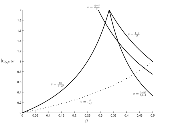
Figure 1. A graph of the various rational functions of $\beta$ appearing in (9) and (10). In Theorems 1.1, 1.2, the limit $(N,\omega)\rightarrow\infty$ is taken with $v_{1}(\beta)\leqslant\log_{N}\omega\leqslant v_{2}(\beta)$. The region of validity is above the dashed curve and below the solid curves. It is a nonempty region for $0<\beta\leqslant 3/7$. As shown here, there are values of $\beta$ for which $v_{1}(\beta)\leqslant 1\leqslant v_{2}(\beta)$, which allows $N\sim\omega$, as in the experimental paper [24, 27, 44, 63, 35, 62, 41, 26]. Moreover, our result includes part of the $\beta>1/3$ self-interaction region. We will explain why we call the $\beta>1/3$ case self-interaction later in this introduction. At the moment, we remark that it is not a coincidence that three restrictions intersect at $\beta=1/3$

We remark that the assumptions in Theorem 1.1 are reasonable assumptions on the initial datum coming from Step A. In [50, (1.10)], a satisfying answer has been found by Lieb, Seiringer, and Yngvason for Step A (Problem 1) in the $\omega_{0,x}\gg\omega_{0,z}$ case. For convenience, set $\omega_{0,z}=1$ in the defocusing $N$-body Hamiltonian (3) in Step A. Let $\mathop{\mathrm{s}cat}(W)$ denote the 3D scattering length of the potential $W$. By [31, Lemma A.1], for $0<\beta\leq 1$ and $a\ll 1$, we have

$$\mathop{\mathrm{s}cat}\left(a\cdot\frac{1}{a^{3\beta}}V\left(\frac{r}{a^{\beta}}\right)\right)\sim\begin{cases}\frac{a}{8\pi}\int_{\mathbb{R}^{3}}V&\text{if }0<\beta<1\\ a\mathop{\mathrm{s}cat}\left(V\right)&\text{if }\beta=1\end{cases}$$

In [50, (1.10)], Lieb, Seiringer, and Yngvason define the quantity $g=g(\omega_{0,x},N,a)$ by

$$g\overset{\mathrm{def}}{=}8\pi a\omega_{0,x}\left(\int\left|h(x)\right|^{4}dx\right)\text{.}$$

Then if $Ng\sim 1$, they proved in [50, Theorem 5.1] that BEC happens in Step A and the Gross-Pitaevskii limit holds. To be specific, they proved that

$$\lim_{N,\omega_{0,x}\rightarrow\infty}\mathop{\mathrm{T}r}\left|\frac{1}{\omega_{0,x}}\gamma_{N,\omega_{0,x}}^{(1)}(0,\frac{x_{1}}{\sqrt{\omega_{0,x}}},z_{1};\frac{x_{1}^{\prime}}{\sqrt{\omega_{0,x}}},z_{1}^{\prime})-h(x_{1})h(x_{1}^{\prime})\phi_{0}(z_{1})\overline{\phi_{0}}(z_{1}^{\prime})\right|=0$$

provided that $\phi_{0}$ is the minimizer to the 1D defocusing NLS energy functional

(13) $$E_{\omega_{z},Ng}=\int_{\mathbb{R}}\left(|\partial_{z}\phi(z)|^{2}+z^{2}|\phi(z)|^{2}+4\pi Ng|\phi(z)|^{4}\right)\,dz$$

subject to the constraint $\|\phi\|_{L^{2}(\mathbb{R})}=1$. Hence, the assumptions in Theorem 1.1 are reasonable assumptions on the initial datum drawn from Step A. To be specific, we have chosen $a=(N\omega)^{-1}$ in the interaction so that $Ng\sim 1$ and assumptions (a), (b) and (c) are the conclusions of [50, Theorem 5.1].

The equivalence of Theorems 1.1 and 1.2 for asymptotically factorized initial data is well-known. In the main part of this paper, we prove Theorem 1.2 in full detail. For completeness, we discuss briefly how to deduce Theorem 1.1 from Theorem 1.2 in Appendix B.

To our knowledge, Theorems 1.1 and 1.2 offer the first rigorous derivation of the 1D focusing cubic NLS (11) from the 3D focusing quantum $N$-body dynamic (6). Moreover, our result covers part of the $\beta>1/3$ self-interaction region in 3D. As pointed out in [28], the study of Step B is of particular interest when $\beta\in\left(1/3,1\right]$ in 3D. The reason is the following. The initial datum coming from Step A is the ground state of (3) with $\omega_{0,x},\omega_{0,z}$ $\neq 0$ and hence is localized in space. We can assume all $N$ particles are in a box of length $1$. Let the effective radius of the pair interaction $V$ be $R_{0},$ then the effective radius of $V\left(\left(N\omega\right)^{\beta}\left(r_{i}-r_{j}\right)\right)$ is about $R_{0}/\left(N\omega\right)^{\beta}$. Thus every particle in the box interacts with $\left(R_{0}/\left(N\omega\right)^{\beta}\right)^{3}\times N$ other particles. Thus, for $\beta>1/3$ and large $N$, every particle interacts with only itself. This exactly matches the Gross-Pitaevskii theory that the many-body effect should be modeled by a strong on-site self-interaction. Therefore, for the mathematical justification of the Gross-Pitaevskii theory, it is of particular interest to prove Theorems 1.1 and 1.2 for self-interaction ($\beta>1/3)$.

A main tool used to prove Theorem 1.2 is the analysis of the BBGKY hierarchy of $\left\{\tilde{\gamma}_{N,\omega}^{(k)}(t)=\frac{1}{\omega^{k}}\gamma_{N,\omega}^{(k)}(t,\frac{\mathbf{x}_{k}}{\sqrt{\omega}},\mathbf{z}_{k};\frac{\mathbf{x}_{k}^{\prime}}{\sqrt{\omega}},\mathbf{z}_{k}^{\prime})\right\}_{k=1}^{N}$ as $N,\omega\rightarrow\infty.$ In the classical setting, deriving mean-field type equations by studying the limit of the BBGKY hierarchy was proposed by Kac and demonstrated by Landford’s work on the Boltzmann equation. In the quantum setting, the usage of the BBGKY hierarchy was suggested by Spohn [60] and has been proven to be successful by Elgart, Erdös, Schlein, and Yau in their fundamental papers [28, 30, 31, 32, 33] which rigorously derives the 3D cubic defocusing NLS from a 3D quantum many-body dynamic with repulsive pair interactions and no trapping. The Elgart-Erdös-Schlein-Yau program consists of two principal parts: in one part, they consider the sequence of the marginal densities $\left\{\gamma_{N}^{(k)}\right\}$ associated with the Hamiltonian evolution $e^{itH_{N}}\psi_{N}(0)$ where

$$H_{N}=\sum_{j=1}^{N}-\triangle_{r_{j}}+\frac{1}{N}\sum_{1\leqslant i<j\leqslant N}N^{3\beta}V(N^{\beta}\left(r_{i}-r_{j}\right))$$

and prove that an appropriate limit of as $N\rightarrow\infty$ solves the 3D Gross-Pitaevskii hierarchy

(14) $$i\partial_{t}\gamma^{(k)}+\sum_{j=1}^{k}\left[\triangle_{r_{k}},\gamma^{(k)}\right]=b_{0}\sum_{j=1}^{k}\mathop{\mathrm{T}r}\nolimits_{r_{k+1}}[\delta(r_{j}-r_{k+1}),\gamma^{(k+1)}],\text{ for all }k\geq 1\,.$$

In another part, they show that hierarchy (14) has a unique solution which is therefore a completely factorized state. However, the uniqueness theory for hierarchy (14) is surprisingly delicate due to the fact that it is a system of infinitely many coupled equations over an unbounded number of variables. In [46], by assuming a space-time bound on the limit of $\left\{\gamma_{N}^{(k)}\right\}$, Klainerman and Machedon gave another uniqueness theorem regarding (14) through a collapsing estimate originating from the multilinear Strichartz estimates and a board game argument inspired by the Feynman graph argument in [31].

The method by Klainerman and Machedon [46] was taken up by Kirkpatrick, Schlein, and Staffilani [45], who derived the 2D cubic defocusing NLS from the 2D quantum many-body dynamic; by Chen and Pavlović [11], who considered the 1D and 2D 3-body repelling interaction problem; by X.C. [18, 19], who investigated the defocusing problem with trapping in 2D and 3D; and by X.C. and J.H. [20], who proved the effectiveness of the defocusing 3D to 2D reduction problem. Such a method has also inspired the study of the general existence theory of hierarchy $\eqref{equation:Gross-Pitaevskii hiearchy without a trap}$, see [13, 14, 10, 36, 59].

One main open problem in Klainerman-Machedon theory is the verification of the uniqueness condition in 3D though it is fully solved in 1D and 2D using trace theorems by Kirkpatrick, Schlein, and Staffilani [45]. In [12], for the 3D defocusing problem without traps, Chen and Pavlović showed that, for $\beta\in(0,1/4)$, the limit of the BBGKY sequence satisfies the uniqueness condition. In [19], X.C. extended and simplified their method to study the 3D trapping problem for $\beta\in(0,2/7].$ X.C. and J.H. [21] then extended the $\beta\in(0,2/7]$ result by X.C. to $\beta\in(0,2/3)$ using $X_{b}$ spaces and Littlewood-Paley theory. The $\beta\in\left(2/3,1\right]$ case is still open.

Recently, using a version of the quantum de finite theorem from [49], Chen, Hainzl, Pavlović, and Seiringer provided an alternative proof to the uniqueness theorem in [31] and showed that it is an unconditional uniqueness result in the sense of NLS theory. With this method, Sohinger derived the 3D defocusing cubic NLS in the periodic case [58]. See also [23, 42].

1.1. Organization of the Paper

We first outline the proof of our main theorem, Theorem 1.2, in §2. The components of the proof are in §3, 4, and 5.

The first main part is the proof of the needed focusing energy estimate, stated and proved as Theorem 3.1 in §3. The main difficulty in establishing the energy estimate is understanding the interplay between two parameters $N$ and $\omega$. On the one hand, as suggested by the experiments [24, 27, 44, 63], in order to have to a BEC in this focusing setting, one has to explore ”the 1D feature” of the 3D focusing $N$-body Hamiltonian (6) which comes from a large $\omega$. At the same time, an $N$ too large would allow the 3D effect to dominate, and one has to avoid this. This suggests that an inequality of the form $N^{v_{1}(\beta)}\leq\omega$ is a natural requirement. On the other hand, according to the uncertainty principle, in 3D, as the $x$-component of the particles’ position becomes more and more determined to be $0$, the $x$-component of the momentum and thus the energy must blow up. Hence the energy of the system is dominated by its $x$-directional part which is in fact infinity as $\omega\rightarrow\infty$. Since the particles are interacting via 3D potential, to avoid the excessive $x$-directional energy being transferred to the $z-$ direction, during the $N,\omega\rightarrow\infty$ process, $\omega$ can not be too large either. Such a problem is totally new and does not exists in the 1D model [22]. It suggests that an inequality of the form $\omega\leq N^{\nu_{2}(\beta)}$ is a natural requirement.

The second main part of the proof is the analysis of the focusing ”$\infty-\infty$” BBGKY hierarchy of $\left\{\tilde{\gamma}_{N,\omega}^{(k)}(t)=\frac{1}{\omega^{k}}\gamma_{N,\omega}^{(k)}(t,\frac{\mathbf{x}_{k}}{\sqrt{\omega}},\mathbf{z}_{k};\frac{\mathbf{x}_{k}^{\prime}}{\sqrt{\omega}},\mathbf{z}_{k}^{\prime})\right\}_{k=1}^{N}$ as $N,\omega\rightarrow\infty$. With our definition, the sequence of the marginal densities $\left\{\tilde{\gamma}_{N,\omega}^{(k)}\right\}_{k=1}^{N}$ satisfies the BBGKY hierarchy

$$i\partial_{t}\tilde{\gamma}_{N,\omega}^{(k)} = \omega\sum_{j=1}^{k}[-\Delta_{x_{j}}+\left|x_{j}\right|^{2},\tilde{\gamma}_{N,\omega}^{(k)}]+\sum_{j=1}^{k}[-\partial_{z_{j}}^{2},\tilde{\gamma}_{N,\omega}^{(k)}]$$

$$+\frac{1}{N}\sum_{1\leqslant i<j\leqslant k}[V_{N,\omega}(r_{i}-r_{j}),\tilde{\gamma}_{N,\omega}^{(k)}]$$

$$+\frac{N-k}{N}\sum_{j=1}^{k}\mathop{\mathrm{T}r}\nolimits_{r_{k+1}}[V_{N,\omega}(r_{j}-r_{k+1}),\tilde{\gamma}_{N,\omega}^{(k+1)}].$$

where $V_{N,\omega}$ is defined in (17). We call it an ”$\infty-\infty$” BBGKY hierarchy because it is not clear whether the term

$$\omega[-\Delta_{x_{j}}+\left|x_{j}\right|^{2},\tilde{\gamma}_{N,\omega}^{(k)}]$$

tends to a limit as $N,\omega\rightarrow\infty$. Since $\tilde{\gamma}_{N,\omega}^{(k)}\$is not a factorized state for $t>0$, one cannot expect the commutator to be zero. This is in strong contrast with the ”$n$D to $n$D” work [1, 28, 30, 31, 32, 33, 11, 18, 12, 19, 58] in which the formal limit of the corresponding BBGKY hierarchy is fairly obvious. With the aforementioned focusing energy estimate, we find that this diverging coefficient is counterbalanced by the limiting structure of the density matrices and establish the weak* compactness and convergence of this focusing BBGKY hierarchy in §4 and §5.

1.2. Acknowledgements

J.H. was supported in part by NSF grant DMS-1200455.

2. Proof of the Main Theorem

We start by setting up some notation for the rest of the paper. Recall $h(x)=\pi^{-\frac{1}{2}}e^{-\left|x\right|^{2}/2}$, which is the ground state for the 2D Hermite operator $-\triangle_{x}+\left|x\right|^{2}$ i.e. it solves $(-2-\Delta_{x}+\left|x\right|^{2})h=0$. Then the normalized ground state eigenfunction $h_{\omega}(x)$ of $-\triangle_{x}+\omega^{2}\left|x\right|^{2}$ is given by $h_{\omega}(x)=\omega^{1/2}h(\omega^{1/2}x)$, i.e. it solves $(-2\omega-\triangle_{x}+\omega^{2}\left|x\right|^{2})h_{\omega}=0$. In particular, $h_{1}=h$. Noticing that both of the convergences (7) and (8) involves scaling, we introduce the rescaled solution

(15) $$\tilde{\psi}_{N,\omega}(t,\mathbf{r}_{N})\overset{\mathrm{def}}{=}\frac{1}{\omega^{N/2}}\psi_{N,\omega}(t,\frac{\mathbf{x}_{N}}{\sqrt{\omega}},\mathbf{z}_{N})$$

and the rescaled Hamiltonian

(16) $$\tilde{H}_{N,\omega}=\left[\sum_{j=1}^{N}-\partial_{z_{j}}^{2}+\omega(-\triangle_{x}+\left|x\right|^{2})\right]+\frac{1}{N}\sum_{1\leq i<j\leq N}V_{N,\omega}(r_{i}-r_{j}),$$

where

(17) $$V_{N,\omega}(r)=N^{3\beta}\omega^{3\beta-1}V\left(\frac{\left(N\omega\right)^{\beta}}{\sqrt{\omega}}x,\left(N\omega\right)^{\beta}z\right).$$

Then

$$(\tilde{H}_{N,\omega}\tilde{\psi}_{N,\omega})(t,\mathbf{x}_{N},\mathbf{z}_{N})=\frac{1}{\omega^{N/2}}(H_{N,\omega}\psi_{N,\omega})(t,\frac{\mathbf{x}_{N}}{\sqrt{\omega}},\mathbf{z}_{N}),$$

and hence when $\psi_{N,\omega}(t)$ is the Hamiltonian evolution given by (6) and $\tilde{\psi}_{N,\omega}$ is defined by (15), we have

$$\tilde{\psi}_{N,\omega}(t,\mathbf{r}_{N})=e^{it\tilde{H}_{N,\omega}}\tilde{\psi}(0,\mathbf{r}_{N})\text{.}$$

If we let $\left\{\tilde{\gamma}_{N,\omega}^{(k)}\right\}_{k=1}^{N}$ be the marginal densities associated with $\tilde{\psi}_{N,\omega}$, then $\left\{\tilde{\gamma}_{N,\omega}^{(k)}\right\}_{k=1}^{N}$ satisfies the ”$\infty-\infty$” focusing BBGKY hierarchy

$$i\partial_{t}\tilde{\gamma}_{N,\omega}^{(k)} = \omega\sum_{j=1}^{k}[-\Delta_{x_{j}}+\left|x_{j}\right|^{2},\tilde{\gamma}_{N,\omega}^{(k)}]+\sum_{j=1}^{k}[-\partial_{z_{j}}^{2},\tilde{\gamma}_{N,\omega}^{(k)}]$$

$$+\frac{1}{N}\sum_{1\leqslant i<j\leqslant k}[V_{N,\omega}(r_{i}-r_{j}),\tilde{\gamma}_{N,\omega}^{(k)}]$$

$$+\frac{N-k}{N}\sum_{j=1}^{k}\mathop{\mathrm{T}r}\nolimits_{r_{k+1}}[V_{N,\omega}(r_{j}-r_{k+1}),\tilde{\gamma}_{N,\omega}^{(k+1)}].$$

We will always take $\omega\geq 1$. For the rescaled marginals $\left\{\tilde{\gamma}_{N,\omega}^{(k)}\right\}_{k=1}^{N}$, we define

(19) $$\tilde{S}_{j}\overset{\mathrm{def}}{=}\left[1-\partial_{z_{j}}^{2}+\omega\left(-\Delta_{x_{j}}+\left|x_{j}\right|^{2}-2\right)\right]^{\frac{1}{2}}.$$

Two immediate properties of $\tilde{S}_{j}$ are the following. On the one hand, $\tilde{S}_{j}^{2}(h_{1}(x_{j})\phi(z_{j}))=h_{1}(x_{j})(1-\partial_{z_{j}}^{2})\phi(z_{j})\,$ and thus the diverging parameter $\omega$ has no consequence when $\tilde{S}_{j}$ is applied to a tensor product function $h_{1}(x_{j})\phi(z_{j})$ for which the $x_{j}$-component rests in the ground state. On the other hand, $\tilde{S}_{j}\geqslant 0$ as an operator because $-\Delta_{x_{j}}+\left|x_{j}\right|^{2}-2\geqslant 0$.

Now, noticing that the eigenvalues of $-\triangle_{x}+\omega^{2}\left|x\right|^{2}$ in 2D are $\left\{2\left(l+1\right)\omega\right\}_{l=0}^{\infty}$, let $P_{l\omega}$ the orthogonal projection onto the eigenspace associated with eigenvalue $2\left(l+1\right)\omega$. That is, $I=\sum_{l=0}^{\infty}P_{l\omega}$ where $I:L^{2}(\mathbb{R}^{3})\rightarrow L^{2}(\mathbb{R}^{3})$. As a matter of notation for our multi-coordinate problem, $P_{l\omega}^{j}$ will refer to the projection in $x_{j}$ coordinate at energy $2\left(l+1\right)\omega$, i.e.

(20) $$I=\prod_{j=1}^{k}\left(\sum_{l=0}^{\infty}P_{l\omega}^{j}\right).$$

In particular, when $\omega=1$, we use simply $P_{l}$. That is, $P_{0}$ denotes the orthogonal projection onto the ground state of $-\Delta_{x}+\left|x\right|^{2}$ and $P_{\geqslant 1}$ means the orthogonal projection onto all higher energy modes of $-\Delta_{x}+\left|x\right|^{2}$ so that $I=P_{0}+P_{\geqslant 1}$, where $I:L^{2}(\mathbb{R}^{3})\rightarrow L^{2}(\mathbb{R}^{3})$. Since we will only use $P_{0}$ and $P_{\geqslant 1}$ for the $\omega=1$ case, we define

$$\mathcal{P}_{0} = P_{0}$$

$$\mathcal{P}_{1} = P_{\geqslant 1}$$

and

(21) $$\mathcal{P}_{\mathbf{\alpha}}=\mathcal{P}_{\alpha_{1}}^{1}\cdots\mathcal{P}_{\alpha_{k}}^{k}$$

for a $k$-tuple $\mathbf{\alpha}=(\alpha_{1},\ldots,\alpha_{k})$ with $\alpha_{j}\in\{0,1\}$ and adopt the notation $|\mathbf{\alpha}|=\alpha_{1}+\cdots+\alpha_{k}$, then

(22) $$I=\sum_{\alpha}\mathcal{P}_{\mathbf{\alpha}}\text{.}$$

We next introduce an appropriate topology on the density matrices as was previously done in [28, 29, 30, 31, 32, 33, 45, 11, 18, 19, 20, 21, 22, 58]. Denote the spaces of compact operators and trace class operators on $L^{2}\left(\mathbb{R}^{3k}\right)$ as $\mathcal{K}_{k}$ and $\mathcal{L}_{k}^{1}$, respectively. Then $\left(\mathcal{K}_{k}\right)^{\prime}=\mathcal{L}_{k}^{1}$. By the fact that $\mathcal{K}_{k}$ is separable, we pick a dense countable subset $\{J_{i}^{(k)}\}_{i\geqslant 1}\subset\mathcal{K}_{k}$ in the unit ball of $\mathcal{K}_{k}$ (so $\|J_{i}^{(k)}\|_{\mathop{\mathrm{o}p}}\leqslant 1$ where $\left\|\cdot\right\|_{\mathop{\mathrm{o}p}}$ is the operator norm). For $\gamma_{1}^{(k)},\gamma_{2}^{(k)}\in\mathcal{L}_{k}^{1}$, we then define a metric $d_{k}$ on $\mathcal{L}_{k}^{1}$ by

$$d_{k}(\gamma_{1}^{(k)},\gamma_{2}^{(k)})=\sum_{i=1}^{\infty}2^{-i}\left|\mathop{\mathrm{T}r}J_{i}^{(k)}\left(\gamma_{1}^{(k)}-\gamma_{2}^{(k)}\right)\right|.$$

A uniformly bounded sequence $\tilde{\gamma}_{N,\omega}^{(k)}\in\mathcal{L}_{k}^{1}$ converges to $\tilde{\gamma}^{(k)}\in\mathcal{L}_{k}^{1}$ with respect to the weak* topology if and only if

$$\lim_{N,\omega\rightarrow\infty}d_{k}(\tilde{\gamma}_{N,\omega}^{(k)},\tilde{\gamma}^{(k)})=0.$$

For fixed $T>0$, let $C\left(\left[0,T\right],\mathcal{L}_{k}^{1}\right)$ be the space of functions of $t\in\left[0,T\right]$ with values in $\mathcal{L}_{k}^{1}$ which are continuous with respect to the metric $d_{k}.$ On $C\left(\left[0,T\right],\mathcal{L}_{k}^{1}\right),$ we define the metric

$$\hat{d}_{k}(\gamma^{(k)}\left(\cdot\right),\tilde{\gamma}^{(k)}\left(\cdot\right))=\sup_{t\in\left[0,T\right]}d_{k}(\gamma^{(k)}\left(t\right),\tilde{\gamma}^{(k)}\left(t\right)),$$

and denote by $\tau_{prod}$ the topology on the space $\oplus_{k\geqslant 1}C\left(\left[0,T\right],\mathcal{L}_{k}^{1}\right)$ given by the product of topologies generated by the metrics $\hat{d}_{k}$ on $C\left(\left[0,T\right],\mathcal{L}_{k}^{1}\right).$

With the above topology on the space of marginal densities, we prove Theorem 1.2. The proof is divided into five steps.

• (Focusing Energy Estimate) We first establish, via an elaborate calculation in Theorem 3.1, that one can compensate the negativity of the interaction in the focusing many-body Hamiltonian (6) by adding a product of $N$ and some constant $\alpha$ depending on $V$, provided that $C_{1}N^{v_{1}(\beta)}\leqslant\omega\leqslant C_{2}N^{v_{2}(\beta)}$ where $C_{1}$ and $C_{2}$ depend solely on $V$. Henceforth, though $H_{N,\omega}$ is not positive-definite, we derive, from the energy condition (12), a $H^{1}$ type energy bound:

  $$\left\langle\psi_{N,\omega},\left(\alpha+N^{-1}H_{N,\omega}-2\omega\right)^{k}\psi_{N,\omega}\right\rangle\geqslant C^{k}\left\|\mathop{\displaystyle\prod}\limits_{j=1}^{k}S_{j}\psi_{N,\omega}\right\|_{L^{2}(\mathbb{R}^{3N})}^{2}$$

  where

  $$S_{j}\overset{\mathrm{def}}{=}(1-\Delta_{x_{j}}+\omega^{2}\left|x_{j}\right|^{2}-2\omega-\partial_{z_{j}}^{2})^{1/2}.$$

  Since the quantity $\left\langle\psi_{N,\omega},\left(H_{N,\omega}-2N\omega\right)^{k}\psi_{N,\omega}\right\rangle$ is conserved by the evolution, via Corollary 3.1, we deduce the a priori bounds, crucial to the analysis of the ”$\infty-\infty$” BBGKY hierarchy (2), on the scaled marginal densities:

  $$\sup_{t}\mathop{\mathrm{T}r}\left(\mathop{\displaystyle\prod}\limits_{j=1}^{k}\tilde{S}_{j}\right)\tilde{\gamma}_{N,\omega}^{(k)}\left(\mathop{\displaystyle\prod}\limits_{j=1}^{k}\tilde{S}_{j}\right)\leqslant C^{k},$$

  $$\sup_{t}\mathop{\mathrm{T}r}\mathop{\displaystyle\prod}\limits_{j=1}^{k}\left(1-\triangle_{r_{j}}\right)\tilde{\gamma}_{N,\omega}^{(k)}\leqslant C^{k},$$

  $$\sup_{t}\mathop{\mathrm{T}r}\mathcal{P}_{\mathbf{\alpha}}\tilde{\gamma}_{N,\omega}^{(k)}\mathcal{P}_{\mathbf{\beta}}\leq C^{k}\omega^{-\frac{1}{2}|\mathbf{\alpha}|-\frac{1}{2}\mathbf{|\beta}|},$$

  where $\mathcal{P}_{\mathbf{\alpha}}$ and $\mathcal{P}_{\mathbf{\beta}}$ are defined as in (21). We remark that the quantity

  $$\mathop{\mathrm{T}r}\left(1-\triangle_{r_{1}}\right)\tilde{\gamma}_{N,\omega}^{(1)}$$

  is not the one particle kinetic energy of the system; the one particle kinetic energy of the system is $\mathop{\mathrm{T}r}\left(1-\omega\triangle_{x_{1}}-\partial_{z_{1}}^{2}\right)\tilde{\gamma}_{N,\omega}^{(1)}$ and grows like $\omega$. This is also in contrast to the $n$D to $n$D work,

• (Compactness of BBGKY). We fix $T>0$ and work in the time-interval $t\in[0,T].$ In Theorem 4.1, we establish the compactness of the BBGKY sequence $\left\{\Gamma_{N,\omega}(t)=\left\{\tilde{\gamma}_{N,\omega}^{(k)}\right\}_{k=1}^{N}\right\}\subset\oplus_{k\geqslant 1}C\left(\left[0,T\right],\mathcal{L}_{k}^{1}\right)$ with respect to the product topology $\tau_{prod}$ even though hierarchy (2) contains attractive interactions and an indefinite $\infty-\infty$. Moreover, in Corollary 4.1, we prove that, to be compatible with the energy bound obtained in Step I, every limit point $\Gamma(t)=\left\{\tilde{\gamma}^{(k)}\right\}_{k=1}^{\infty}$ must take the form

  $$\tilde{\gamma}^{(k)}\left(t,\left(\mathbf{x}_{k},\mathbf{z}_{k}\right);\left(\mathbf{x}_{k}^{\prime},\mathbf{z}_{k}^{\prime}\right)\right)=\left(\mathop{\displaystyle\prod}\limits_{j=1}^{k}h_{1}\left(x_{j}\right)h_{1}\left(x_{j}^{\prime}\right)\right)\tilde{\gamma}_{z}^{(k)}(t,\mathbf{z}_{k};\mathbf{z}_{k}^{\prime}),$$

  where $\tilde{\gamma}_{z}^{(k)}=\mathop{\mathrm{T}r}_{x}\tilde{\gamma}^{(k)}$ is the $z$-component of $\tilde{\gamma}^{(k)}.$

• (Limit points of BBGKY satisfy GP). In Theorem 5.1, we prove that if $\Gamma(t)=\left\{\tilde{\gamma}^{(k)}\right\}_{k=1}^{\infty}$ is a $C_{1}N^{v_{1}(\beta)}\leqslant\omega\leqslant C_{2}N^{v_{2}(\beta)}$ limit point of $\left\{\Gamma_{N,\omega}(t)=\left\{\tilde{\gamma}_{N,\omega}^{(k)}\right\}_{k=1}^{N}\right\}$ with respect to the product topology $\tau_{prod}$, then $\left\{\tilde{\gamma}_{z}^{(k)}=\mathop{\mathrm{T}r}_{x}\tilde{\gamma}^{(k)}\right\}_{k=1}^{\infty}$ is a solution to the focusing coupled Gross-Pitaevskii (GP) hierarchy subject to initial data $\tilde{\gamma}_{z}^{(k)}\left(0\right)=\left|\phi_{0}\right\rangle\left\langle\phi_{0}\right|^{\otimes k}$ with coupling constant $b_{0}=$ $\left|\int V\left(r\right)dr\right|$, which written in differential form, is

  (23) $$i\partial_{t}\tilde{\gamma}_{z}^{(k)}=\sum_{j=1}^{k}\left[-\partial_{z_{j}}^{2},\tilde{\gamma}_{z}^{(k)}\right]-b_{0}\sum_{j=1}^{k}\mathop{\mathrm{T}r}\nolimits_{z_{k+1}}\mathop{\mathrm{T}r}\nolimits_{x}\left[\delta\left(r_{j}-r_{k+1}\right),\tilde{\gamma}^{(k+1)}\right].$$

  Together with the limiting structure concluded in Corollary 4.1, we can further deduce that $\left\{\tilde{\gamma}_{z}^{(k)}=\mathop{\mathrm{T}r}_{x}\tilde{\gamma}^{(k)}\right\}_{k=1}^{\infty}$ is a solution to the 1D focusing GP hierarchy subject to initial data $\tilde{\gamma}_{z}^{(k)}\left(0\right)=\left|\phi_{0}\right\rangle\left\langle\phi_{0}\right|^{\otimes k}$ with coupling constant $b_{0}\left(\int\left|h_{1}\left(x\right)\right|^{4}dx\right)$, which, written in differential form, is

  (24) $$i\partial_{t}\tilde{\gamma}_{z}^{(k)}=\sum_{j=1}^{k}\left[-\partial_{z_{j}}^{2},\tilde{\gamma}_{z}^{(k)}\right]-b_{0}\left(\int\left|h_{1}\left(x\right)\right|^{4}dx\right)\sum_{j=1}^{k}\mathop{\mathrm{T}r}\nolimits_{z_{k+1}}\left[\delta\left(z_{j}-z_{k+1}\right),\tilde{\gamma}_{z}^{(k+1)}\right].$$

• (GP has a unique solution). When $\tilde{\gamma}_{z}^{(k)}\left(0\right)=\left|\phi_{0}\right\rangle\left\langle\phi_{0}\right|^{\otimes k},$ we know one solution to the 1D focusing GP hierarchy (24), namely $\left|\phi\right\rangle\left\langle\phi\right|^{\otimes k}$ if $\phi$ solves the 1D focusing NLS (11). Since we have proven the a priori bound

  $$\sup_{t}\mathop{\mathrm{T}r}\left(\mathop{\displaystyle\prod}\limits_{j=1}^{k}\left\langle\partial_{z_{j}}\right\rangle\right)\tilde{\gamma}_{z}^{(k)}\left(\mathop{\displaystyle\prod}\limits_{j=1}^{k}\left\langle\partial_{z_{j}}\right\rangle\right)\leqslant C^{k},$$

  A trace theorem then shows that $\left\{\tilde{\gamma}_{z}^{(k)}\right\}$ verifies the requirement of the following uniqueness theorem and hence we conclude that $\tilde{\gamma}_{z}^{(k)}=\left|\phi\right\rangle\left\langle\phi\right|^{\otimes k}$.

Theorem 2.1 ([22, Theorem 1.3]).

Let

$$B_{j,k+1}\gamma_{z}^{(k+1)}=\mathop{\mathrm{T}r}\nolimits_{z_{k+1}}\left[\delta\left(z_{j}-z_{k+1}\right),\gamma_{z}^{(k+1)}\right].$$

If $\left\{\gamma_{z}^{(k)}\right\}_{k=1}^{\infty}$ solves the 1D focusing GP hierarchy (24) subject to zero initial data and the space-time bound

(25) $$\int_{0}^{T}\left\|\left(\mathop{\displaystyle\prod}\limits_{j=1}^{k}\left\langle\partial_{z_{j}}\right\rangle^{\varepsilon}\left\langle\partial_{z_{j}^{\prime}}\right\rangle^{\varepsilon}\right)B_{j,k+1}\gamma_{z}^{(k+1)}(t,\mathbf{\cdot};\mathbf{\cdot})\right\|_{L_{\mathbf{z,z}^{\prime}}^{2}}dt\leqslant C^{k}$$

for some $\varepsilon,C>0$ and all $1\leqslant j\leqslant k.$ Then $\forall k,t\in[0,T]$, $\gamma_{z}^{(k+1)}=0.$

Thus the compact sequence $\left\{\Gamma_{N,\omega}(t)=\left\{\tilde{\gamma}_{N,\omega}^{(k)}\right\}_{k=1}^{N}\right\}$ has only one $C_{1}N^{v_{1}(\beta)}\leqslant\omega\leqslant C_{2}N^{v_{2}(\beta)}$ limit point, namely

$$\tilde{\gamma}^{(k)}=\mathop{\displaystyle\prod}\limits_{j=1}^{k}h_{1}\left(x_{j}\right)h_{1}(x_{j}^{\prime})\phi(t,z_{j})\overline{\phi}(t,z_{j}^{\prime})\,.$$

We then infer from the definition of the topology that as trace class operators

$$\tilde{\gamma}_{N,\omega}^{(k)}\rightarrow\mathop{\displaystyle\prod}\limits_{j=1}^{k}h_{1}\left(x_{j}\right)h_{1}(x_{j}^{\prime})\phi(t,z_{j})\overline{\phi}(t,z_{j}^{\prime})\text{ weak*.}$$

• (Weak* convergence upgraded to strong). Since the limit concluded in Step IV is an orthogonal projection, the well-known argument in [33] upgrades the weak* convergence to strong. In fact, testing the sequence against the compact observable

  $$J^{(k)}=\mathop{\displaystyle\prod}\limits_{j=1}^{k}h_{1}\left(x_{j}\right)h_{1}(x_{j}^{\prime})\phi(t,z_{j})\overline{\phi}(t,z_{j}^{\prime}),$$

  and noticing the fact that $\left(\tilde{\gamma}_{N,\omega}^{(k)}\right)^{2}\leqslant\tilde{\gamma}_{N,\omega}^{(k)}$ since the initial data is normalized, we see that as Hilbert-Schmidt operators

  $$\tilde{\gamma}_{N,\omega}^{(k)}\rightarrow\mathop{\displaystyle\prod}\limits_{j=1}^{k}h_{1}\left(x_{j}\right)h_{1}(x_{j}^{\prime})\phi(t,z_{j})\overline{\phi}(t,z_{j}^{\prime})\text{ strongly.}$$

  Since $\mathop{\mathrm{T}r}\tilde{\gamma}_{N,\omega}^{(k)}=\mathop{\mathrm{T}r}\tilde{\gamma}^{(k)},$ we deduce the strong convergence

  $$\lim_{\begin{subarray}{c}N,\omega\rightarrow\infty\\ C_{1}N^{v_{1}(\beta)}\leqslant\omega\leqslant C_{2}N^{v_{2}(\beta)}\end{subarray}}\mathop{\mathrm{T}r}\left|\tilde{\gamma}_{N,\omega}^{(k)}(t,\mathbf{x}_{k},\mathbf{z}_{k};\mathbf{x}_{k}^{\prime},\mathbf{z}_{k}^{\prime})-\mathop{\displaystyle\prod}\limits_{j=1}^{k}h_{1}\left(x_{j}\right)h_{1}(x_{j}^{\prime})\phi(t,z_{j})\overline{\phi}(t,z_{j}^{\prime})\right|=0,$$

  via the Grümm’s convergence theorem [56, Theorem 2.19].

3. Focusing Energy Estimate

We find it more convenient to prove the energy estimate for $\psi_{N,\omega}$ and then convert it by scaling to an estimate for $\tilde{\psi}_{N,\omega}$ (see (15)). Note that, as an operator, we have the positivity:

$$-\Delta_{x_{j}}+\omega^{2}\left|x_{j}\right|^{2}-2\omega\geqslant 0$$

Define

$$S_{j}\overset{\mathrm{def}}{=}(1-\Delta_{x_{j}}+\omega^{2}\left|x_{j}\right|^{2}-2\omega-\partial_{z_{j}}^{2})^{1/2}=(1-2\omega-\Delta_{r_{j}}+\omega^{2}\left|x_{j}\right|^{2})^{1/2},$$

and write

$$S^{(k)}=\mathop{\displaystyle\prod}\limits_{j=1}^{k}S_{j}.$$

Theorem 3.1 (energy estimate).

For $\beta\in(0,\frac{3}{7})$, let

(26) $$v_{E}(\beta)=\min\left(\frac{1-\beta}{\beta},\frac{\frac{3}{5}-\beta}{\beta-\frac{1}{5}}\mathbf{1}_{\beta\geqslant\frac{1}{5}}+\infty\cdot\mathbf{1}_{\beta<\frac{1}{5}},\frac{\frac{7}{8}-\beta}{\beta}\right)\text{.}$$

There are constants $C_{1}=C_{1}(\|V\|_{L^{1}},\|V\|_{L^{\infty}})$, $C_{2}=C_{2}(\|V\|_{L^{1}},\|V\|_{L^{\infty}})$, and absolute constant $C_{3}$, and for each $k\in\mathbb{N}$, there is an integer $N_{0}(k)$, such that for any $k\in\mathbb{N}$, $N\geq N_{0}(k)$ and $\omega$ which satisfy

(27) $$C_{1}N^{v_{1}(\beta)}\leqslant\omega\leqslant C_{2}N^{v_{E}(\beta)},$$

there holds

(28) $$\langle(\alpha+N^{-1}H_{N,\omega}-2\omega)^{k}\psi,\psi\rangle\geqslant\frac{1}{2^{k}}(\|S^{(k)}\psi\|_{L^{2}}^{2}+N^{-1}\|S_{1}S^{(k-1)}\psi\|_{L^{2}}^{2}),$$

where

$$\alpha=C_{3}\|V\|_{L^{1}}^{2}+1.$$

Proof.

For smoothness of presentation, we postpone the proof to §3.1.    

Recall the rescaled operator (19)

$$\tilde{S}_{j}=\left[1-\partial_{z_{j}}^{2}+\omega\left(-\Delta_{x_{j}}+\left|x_{j}\right|^{2}-2\right)\right]^{\frac{1}{2}},$$

we notice that

$$(S_{j}\psi)(t,\mathbf{x}_{N},\mathbf{z}_{N})=\omega^{N/2}(\tilde{S}_{j}\tilde{\psi})(t,\sqrt{\omega}\mathbf{x}_{N},\mathbf{z}_{N})\,,$$

if $\tilde{\psi}_{N,\omega}$ is defined via (15). Thus we can convert the conclusion of Theorem 3.1 into statements about $\tilde{\psi}_{N,\omega}$, $\tilde{S}_{j}$, and $\tilde{\gamma}_{N,\omega}^{(k)}$ which we will utilize in the rest of the paper.

Corollary 3.1.

Define

$$\tilde{S}^{(k)}=\prod_{j=1}^{k}\tilde{S}_{j}\text{, }L^{(k)}=\prod_{j=1}^{k}\left\langle\nabla_{r_{j}}\right\rangle$$

Assume $C_{1}N^{v_{1}(\beta)}\leqslant\omega\leqslant C_{2}N^{v_{E}(\beta)}$. Let $\tilde{\psi}_{N,\omega}(t)=e^{it\tilde{H}_{N,\omega}}\tilde{\psi}_{N,\omega}(0)$ and $\{\tilde{\gamma}_{N,\omega}^{(k)}(t)\}$ be the associated marginal densities, then for all $\omega\geqslant 1$ , $k\geqslant 0$, $N\$large enough, we have the uniform-in-time bound

(29) $$\mathop{\mathrm{T}r}\tilde{S}^{(k)}\tilde{\gamma}_{N,\omega}^{(k)}\tilde{S}^{(k)}=\left\|\tilde{S}^{(k)}\tilde{\psi}_{N,\omega}(t)\right\|_{L^{2}(\mathbb{R}^{3N})}^{2}\leqslant C^{k}.$$

Consequently,

(30) $$\mathop{\mathrm{T}r}L^{(k)}\tilde{\gamma}_{N,\omega}^{(k)}L^{(k)}=\left\|L^{(k)}\tilde{\psi}_{N,\omega}(t)\right\|_{L^{2}(\mathbb{R}^{3N})}^{2}\leqslant C^{k},$$

and

(31) $$\|\mathcal{P}_{\mathbf{\alpha}}\tilde{\psi}_{N,\omega}\|_{L^{2}(\mathbb{R}^{3N})}\leqslant C^{k}\omega^{-|\mathbf{\alpha}|/2}\,\text{, }\left|\mathop{\mathrm{T}r}\mathcal{P}_{\mathbf{\alpha}}\tilde{\gamma}_{N,\omega}^{(k)}\mathcal{P}_{\mathbf{\beta}}\right|\leqslant C^{k}\omega^{-\frac{1}{2}|\mathbf{\alpha}|-\frac{1}{2}\mathbf{|\beta}|}$$

where $\mathcal{P}_{\mathbf{\alpha}}$ and $\mathcal{P}_{\mathbf{\beta}}$ are defined as in (21).

Proof.

Substituting (15) into estimate (28) and rescaling, we obtain

$$\left\|\tilde{S}^{(k)}\tilde{\psi}_{N,\omega}(t)\right\|_{L^{2}(\mathbb{R}^{3N})}^{2}\leqslant C^{k}\langle\tilde{\psi}_{N,\omega}(t),(\alpha+N^{-1}\tilde{H}_{N,\omega}-2\omega)^{k}\tilde{\psi}_{N,\omega}(t)\rangle.$$

The quantity on the right hand side is conserved, therefore

$$=C^{k}\langle\tilde{\psi}_{N,\omega}(0),(\alpha+N^{-1}\tilde{H}_{N,\omega}-2\omega)^{k}\tilde{\psi}_{N,\omega}(0)\rangle.$$

Apply the binomial theorem twice,

$$\leqslant C^{k}\sum_{j=0}^{k}\begin{pmatrix}k\\ j\end{pmatrix}\alpha^{j}\langle\tilde{\psi}_{N,\omega}(0),(N^{-1}\tilde{H}_{N,\omega}-2\omega)^{k-j}\tilde{\psi}_{N,\omega}(0)\rangle$$

$$\leqslant C^{k}\sum_{j=0}^{k}\begin{pmatrix}k\\ j\end{pmatrix}\alpha^{j}\left(C\right)^{k-j}$$

$$= C^{k}\left(\alpha+C\right)^{k}\leqslant\tilde{C}^{k}.$$

where we used condition (12) in the second to last line. So we have proved (29). Putting (29) and (72) together, estimate (30) then follows. The first inequality of (31) follows from (29) and (74). By Lemma A.5, $\mathop{\mathrm{T}r}\mathcal{P}_{\mathbf{\alpha}}\tilde{\gamma}_{N,\omega}^{(k)}\mathcal{P}_{\mathbf{\beta}}=\langle\mathcal{P}_{\mathbf{\alpha}}\tilde{\psi}_{N,\omega},\mathcal{P}_{\mathbf{\beta}}\tilde{\psi}_{N,\omega}\rangle$, so the second inequality of (31) follows by Cauchy-Schwarz.    

3.1. Proof of the Focusing Energy Estimate

Note that

$$N^{-1}H_{N,\omega}-2\omega=N^{-1}\sum_{i=1}^{N}(-\Delta_{r_{i}}+\omega^{2}|x_{i}|^{2}-2\omega)+N^{-2}\omega^{-1}\sum_{1\leq i<j\leq N}V_{N\omega}(r_{i}-r_{j}),$$

where we have used the notation

$$V_{N\omega}(r)=(N\omega)^{3\beta}V((N\omega)^{\beta}r).$$

Define

$$H_{Kij}=(\alpha-\Delta_{r_{i}}+\omega^{2}|x_{i}|^{2}-2\omega)+(\alpha-\Delta_{r_{j}}+\omega^{2}|x_{j}|^{2}-2\omega)$$

where the $K$ stands for “kinetic” and

$$H_{Iij}=\omega^{-1}V_{N\omega ij}=\omega^{-1}V_{N\omega}(r_{i}-r_{j})$$

where the $I$ is for “interaction”. If we write

$$H_{ij}=H_{Kij}+H_{Iij},$$

then

(32) $$\alpha+N^{-1}H_{N,\omega}-2\omega=\frac{1}{2}N^{-2}\sum_{1\leq i\neq j\leq N}H_{ij}=N^{-2}\sum_{1\leq i<j\leq N}H_{ij}.$$

We will first prove Theorem 3.1 for $k=1$ and $k=2$. Then, by a two-step induction (result known for $k$ implies result for $k+2$), we establish the general case. Before we proceed, we prove some estimates regarding the Hermite operator.

3.1.1. Estimates Needed to Prove Theorem 3.1

Lemma 3.1.

Let $P_{l\omega}$ be defined as in (20). There is a constant independent of $\ell$ and $\omega$ such that

(33) $$\|P_{\ell\omega}f\|_{L_{x}^{\infty}}\leqslant C\omega^{1/2}\|f\|_{L_{x}^{2}}.$$

with constant independent of $\ell$ and $\omega$.

Proof.

This estimate has more than one proof. It is a special result in 2D. It does not follow from the Strichartz estimates. For a modern argument which proves the estimate for general at most quadratic potentials, see [48, Corollary 2.2]. In the special case of the quantum harmonic oscillator, one can also use a special property of 2D Hermite projection kernels to yield a direct proof without using Littlewood-Paley theory – see [64, Lemma 3.2.2], [16, Remark 8].    

Lemma 3.2.

There is an absolute constant $C_{3}>0$ and a constant $C_{1}=C\left(\|V\|_{L^{1}},\|V\|_{L^{\infty}}\right)$ such that if

$$\omega\geq C_{1}N^{\beta/(1-\beta)}$$

then

$$\frac{1}{\omega}\int\left|V_{N\omega}(r_{1}-r_{2})\right|\left|\psi(r_{1},r_{2})\right|^{2}dr_{1}$$

$$\leqslant \frac{1}{100}\left\langle\psi(r_{1},r_{2}),(-\Delta_{r_{1}}+\omega^{2}|x_{1}|^{2}-2\omega)\psi(r_{1},r_{2})\right\rangle_{r_{1}}+C_{3}\left\|V\right\|_{L^{1}}^{2}\left\|\psi(r_{1},r_{2})\right\|_{L_{r_{1}}^{2}}^{2}.$$

The above estimate is performed in one coordinate only (taken to be $r_{1}$), and the other coordinate $r_{2}$ are effectively “frozen”. In particular, let

$$f(r_{2},\ldots,r_{N})=\int\left|V_{N\omega}(r_{1}-r_{2})\right|\left|\psi_{1}(r_{1},\ldots,r_{N})\right|\left|\psi_{2}(r_{1},\ldots,r_{N})\right|dr_{1}$$

Then

(35) $$f(r_{2},\ldots,r_{N})\lesssim\omega\|S_{1}\psi_{1}(r_{1},\cdots,r_{N})\|_{L_{r_{1}}^{2}}\|S_{1}\psi_{2}(r_{1},\cdots,r_{N})\|_{L_{r_{1}}^{2}},$$

The implicit constant in $\lesssim$ is an absolute constant times $\|V\|_{L^{1}}+\|V\|_{L^{\infty}}$.

Proof.

By Cauchy-Schwarz,

$$\int|V_{N\omega 12}|\,|\psi_{1}|\,|\psi_{2}|dr_{1}\leqslant\left(\int|V_{N\omega 12}||\psi_{1}|^{2}\,dr_{1}\right)^{1/2}\left(\int|V_{N\omega 12}||\psi_{2}|^{2}\,dr_{1}\right)^{1/2}.$$

Thus, assuming (3.2) and using the facts that

$$S_{1}^{2} \geqslant 1,$$

$$S_{1}^{2} \geqslant (-\Delta_{r_{1}}+\omega^{2}|x_{1}|^{2}-2\omega),$$

we obtain (35). So we only need to to prove (3.2).

Taking $P_{l\omega}$ to be the projection onto the $x_{1}$ component, we decompose $\psi$ into ground state, middle energies, and high energies as follows:

$$\psi=P_{0\omega}\psi+\sum_{\ell=1}^{e-1}P_{\ell\omega}\psi+P_{\geq e\omega}\psi$$

where $e$ is an integer, and the optimal choice of $e$ is determined below. It then suffices to bound

(36) $$A_{\text{low}}\ \overset{\mathrm{def}}{=}\frac{1}{\omega}\int|V_{N\omega}(r_{1}-r_{2})||P_{0\omega}\psi(r_{1},r_{2})|^{2}dr_{1}$$

(37) $$A_{\text{mid}}\ \overset{\mathrm{def}}{=}\frac{1}{\omega}\int|V_{N\omega}(r_{1}-r_{2})||\sum_{\ell=2}^{e-1}P_{\ell\omega}\psi(r_{1},r_{2})|^{2}dr_{1}$$

(38) $$A_{\text{high}}\ \overset{\mathrm{def}}{=}\frac{1}{\omega}\int|V_{N\omega}(r_{1}-r_{2})||P_{\geq e\omega}\psi(r_{1},r_{2})|^{2}dr_{1}$$

For each estimate, we will only work in the $r_{1}=(x_{1},z_{1})$ component, and thus will not even write the $r_{2}$ variable. First we consider (36).

$$A_{\text{low}}\ \leqslant\frac{1}{\omega}\|V_{N\omega}\|_{L^{1}}\|P_{0\omega}\psi\|_{L_{x}^{\infty}L_{z}^{\infty}}^{2}$$

By the standard 1D Sobolev-type estimate

$$A_{\text{low}}\lesssim\frac{1}{\omega}\|V\|_{L^{1}}\|P_{0\omega}\partial_{z}\psi\|_{L_{x}^{\infty}L_{z}^{2}}\|P_{0\omega}\psi\|_{L_{x}^{\infty}L_{z}^{2}}$$

Then use the estimate (33)

$$A_{\text{low}}\ \lesssim\|V\|_{L^{1}}\|P_{0\omega}\partial_{z}\psi\|_{L_{r}^{2}}\|P_{0\omega}\psi\|_{L_{r}^{2}}$$

$$\lesssim\|V\|_{L^{1}}\|\partial_{z}\psi\|_{L^{2}}\|\psi\|_{L^{2}}$$

$$\lesssim\epsilon\|\partial_{z}\psi\|_{L^{2}}^{2}+\frac{\|V\|_{L^{1}}^{2}}{\epsilon}\|\psi\|_{L^{2}}^{2}\text{.}$$

Since, $(-\Delta_{r}+\omega^{2}|x|^{2}-2\omega)$ is a sum of two positive operators, namely, $-\Delta_{x}+\omega^{2}|x|^{2}-2\omega$ and $-\partial_{z}^{2}$, we conclude the estimate for $A_{\text{low}}$.

Now consider the middle harmonic energies given by (37), and we aim to estimate $A_{\text{mid}}$. For any $\ell\geq 1$, we have

$$\|P_{\ell\omega}\psi\|_{L_{z}^{\infty}L_{x}^{\infty}}\leq\|P_{\ell\omega}\partial_{z}\psi\|_{L_{z}^{2}L_{x}^{\infty}}^{1/2}\|P_{\ell\omega}\psi\|_{L_{z}^{2}L_{x}^{\infty}}^{1/2}$$

By (33),

$$\|P_{\ell\omega}\psi\|_{L_{z}^{\infty}L_{x}^{\infty}} \lesssim\omega^{1/2}\|P_{\ell\omega}\partial_{z}\psi\|_{L_{z}^{2}L_{x}^{2}}^{1/2}\|P_{\ell\omega}\psi\|_{L_{z}^{2}L_{x}^{2}}^{1/2}$$

$$=\omega^{1/4}\|P_{\ell\omega}\partial_{z}\psi\|_{L^{2}}^{1/2}(\|P_{\ell\omega}\psi\|_{L^{2}}\ell^{1/2}\omega^{1/2})^{1/2}\,\ell^{-1/4}$$

$$=\omega^{1/4}\|P_{\ell\omega}\partial_{z}\psi\|_{L_{r}^{2}}^{1/2}\|P_{\ell\omega}(-\Delta_{x}+\omega^{2}|x|^{2}-2\omega)^{1/2}\psi\|_{L^{2}}^{1/2}\,\ell^{-1/4}$$

Sum over $1\leq\ell\leq e-1$, and do Hölder with exponents $4$, $4$, and $2$:

$$\sum_{\ell=1}^{e-1}\|P_{\ell\omega}\psi\|_{L_{z}^{\infty}L_{x}^{\infty}} \lesssim\omega^{1/4}\left(\sum_{\ell=1}^{e-1}\|P_{\ell\omega}\partial_{z}\psi\|_{L^{2}}^{2}\right)^{1/4}$$

$$\quad\quad\times\left(\sum_{\ell=1}^{e-1}\|P_{\ell\omega}(-\Delta_{x}+\omega^{2}|x|^{2}-2\omega)^{1/2}\psi\|_{L^{2}}^{2}\right)^{1/4}\left(\sum_{\ell=1}^{e}\ell^{-1/2}\right)^{1/2}$$

$$\lesssim\omega^{1/4}e^{1/4}\|\partial_{z}\psi\|_{L^{2}}^{1/2}\|(-\Delta_{x}+\omega^{2}|x|^{2}-2\omega)^{1/2}\psi\|_{L^{2}}^{1/2}$$

Applying this to estimate (37),

$$A_{\text{mid}}\lesssim\omega^{-1/2}e^{1/2}\|V\|_{L^{1}}\|\partial_{z}\psi\|_{L^{2}}\|(-\Delta_{x}+\omega^{2}|x|^{2}-2\omega)^{1/2}\psi\|_{L^{2}}$$

Take $e$ so that $\omega^{-1/2}e^{1/2}\|V\|_{L^{1}}=\epsilon$, i.e.

(39) $$e=\frac{\epsilon^{2}}{\|V\|_{L^{1}}^{2}}\omega$$

and then we have

$$A_{\text{mid}}\ \lesssim\epsilon\|\partial_{z}\psi\|_{L^{2}}^{2}+\epsilon\|(-\Delta_{x}+\omega^{2}|x|^{2}-2\omega)^{1/2}\psi\|_{L^{2}}^{2}$$

For (38),

$$A_{\text{high}} \lesssim\omega^{-1}\|V_{N\omega}\|_{L^{\infty}}\|P_{\geq e\omega}\psi\|_{L^{2}}^{2}$$

$$\lesssim\omega^{-2}e^{-1}\|V_{N\omega}\|_{L^{\infty}}\|e^{1/2}\omega^{1/2}P_{\geq e\omega}\psi\|_{L^{2}}^{2}$$

$$\lesssim\omega^{-2}e^{-1}(N\omega)^{3\beta}\|V\|_{L^{\infty}}\|(-\Delta_{x}+\omega^{2}|x|^{2}-2\omega)^{1/2}\psi\|_{L^{2}}^{2}$$

We need

$$\omega^{-2}e^{-1}(N\omega)^{3\beta}\leq\epsilon$$

Substituting the specification of $e$ given by (39), we obtain

$$N^{3\beta}\omega^{3\beta-3}\leq\frac{\epsilon^{2}}{\|V\|_{L^{1}}^{2}\|V\|_{L^{\infty}}}.$$

That is $\omega\geq C_{1}N^{\beta/(1-\beta)}$ as required in the statement of Lemma 3.2.    

In the following lemma, we have excited state estimates and ground state estimates, and the ground state estimates are weaker (involve a loss of $\omega^{1/2}$)

Lemma 3.3.

Taking $\psi=\psi(r)$, we have the following “excited state” estimate:

(40) $$\|\omega^{1/2}P_{\geq 1\omega}\psi\|_{L^{2}}+\|\omega|x|P_{\geq 1\omega}\psi\|_{L^{2}}+\|\nabla_{r}P_{\geq 1\omega}\psi\|_{L^{2}}\lesssim\|S\psi\|_{L^{2}},$$

and the following “ground state” estimate

(41) $$\|\omega^{1/2}P_{0\omega}\psi\|_{L^{2}}+\|\omega|x|P_{0\omega}\psi\|_{L^{2}}+\|\nabla_{r}P_{0\omega}\psi\|_{L^{2}}\lesssim\omega^{1/2}\|\psi\|_{L^{2}}$$

We are, however, spared from the $\omega^{1/2}$ loss when working only with the $z$-derivative

(42) $$\|\partial_{z}P_{0\omega}\psi\|_{L^{2}}\lesssim\|S\psi\|_{L^{2}}$$

Putting the excited state and ground state estimates together gives

(43) $$\|\omega^{1/2}\psi\|_{L^{2}}+\|\omega|x|\psi\|_{L^{2}}+\|\nabla_{r}\psi\|_{L^{2}}\lesssim\omega^{1/2}\|S\psi\|_{L^{2}}$$

Proof.

For the excited state estimates, we note

$$0\leq\langle P_{\geq 1\omega}\psi,(-\Delta_{x}+\omega^{2}|x|^{2}-4\omega)P_{\geq 1\omega}\psi\rangle$$

Adding $\frac{3}{2}\|\partial_{z}P_{\geq 1\omega}\psi\|_{L^{2}}^{2}+\frac{1}{2}\|\nabla_{x}P_{\geq 1\omega}\psi\|_{L^{2}}^{2}+\frac{1}{2}\|\omega|x|P_{\geq 1\omega}\psi\|_{L^{2}}^{2}+\|\omega^{1/2}P_{\geq 1\omega}\psi\|_{L^{2}}^{2}$ to both sides

$$\frac{3}{2}\|\partial_{z}P_{\geq 1\omega}\psi\|_{L^{2}}^{2}+\frac{1}{2}\|\nabla_{x}P_{\geq 1\omega}\psi\|_{L^{2}}^{2}+\frac{1}{2}\|\omega|x|P_{\geq 1\omega}\psi\|_{L^{2}}^{2}+\|\omega^{1/2}P_{\geq 1\omega}\psi\|_{L^{2}}^{2}$$

$$\leq\frac{3}{2}\langle P_{\geq 1\omega}\psi,(-\Delta_{r}+\omega^{2}|x|^{2}-2\omega)P_{\geq 1\omega}\psi\rangle$$

This proves (40). The ground state estimate (41) and (42) are straightforward from the explicit definition of $P_{0\omega}$ which is merely projecting onto a Gaussian.    

Lemma 3.4.

We have the following estimates:

(44) $$\||V_{N\omega 12}|^{1/2}S_{1}P_{0\omega}^{1}\psi_{2}\|_{L_{r_{1}}^{2}} \lesssim \omega^{\frac{1}{2}}N^{\frac{1}{4}}\|S_{1}\psi_{2}\|_{L^{2}}^{1/2}\left(N^{-\frac{1}{4}}\|S_{1}^{2}\psi_{2}\|_{L^{2}}^{1/2}\right)$$

(45) $$\||V_{N\omega 12}|^{1/2}S_{1}P_{\geqslant 1\omega}^{1}\psi_{2}\|_{L_{r_{1}}^{2}} \lesssim N^{\frac{\beta}{2}+\frac{1}{2}}\omega^{\frac{\beta}{2}}\left(N^{-1/2}\|S_{1}^{2}\psi_{2}\|_{L_{r_{1}}^{2}}\right)$$

In particluar, if $\omega\geqslant C_{1}N^{\beta/(1-\beta)}$ then

$$\int_{r_{1}}|V_{N\omega 12}||\psi_{1}||S_{1}\psi_{2}|\,dr_{1}$$

$$\lesssim \omega N^{\frac{1}{4}}\left\|S_{1}\psi_{1}\right\|_{L^{2}}\left\|S_{1}\psi_{2}\right\|_{L^{2}}^{\frac{1}{2}}N^{-\frac{1}{4}}\left\|S_{1}^{2}\psi_{2}\right\|_{L^{2}}^{\frac{1}{2}}$$

$$+\left(N\omega\right)^{\frac{\beta}{2}+\frac{1}{2}}\left\|S_{1}\psi_{1}\right\|_{L^{2}}N^{-\frac{1}{2}}\left\|S_{1}^{2}\psi_{2}\right\|_{L^{2}}$$

Proof.

To prove (3.4), substituting $\psi_{2}=P_{0\omega}^{1}\psi_{2}+P_{\geq 1\omega}^{1}\psi_{2}$, we obtain

$$\int_{r_{1}}|V_{N\omega 12}||\psi_{1}||S_{1}\psi_{2}|dr_{1}\lesssim F_{1}+F_{2}$$

where

$$F_{1} = \int_{r_{1}}|V_{N\omega 12}||\psi_{1}||P_{0\omega}^{1}S_{1}\psi_{2}|dr_{1}$$

$$\leqslant \||V_{N\omega 12}|^{1/2}\psi_{1}\|_{L_{r_{1}}^{2}}\||V_{N\omega 12}|^{1/2}P_{0\omega}^{1}S_{1}\psi_{2}\|_{L_{r_{1}}^{2}}$$

$$\leqslant \omega^{1/2}\|S_{1}\psi_{1}\|_{L_{r_{1}}^{2}}\||V_{N\omega 12}|^{1/2}P_{0\omega}^{1}S_{1}\psi_{2}\|_{L_{r_{1}}^{2}}$$

$$F_{2} = \int_{r_{1}}|V_{N\omega 12}||\psi_{1}||P_{\geq 1\omega}^{1}S_{1}\psi_{2}|dr_{1}$$

$$\leqslant \omega^{1/2}\|S_{1}\psi_{1}\|_{L_{r_{1}}^{2}}\||V_{N\omega 12}|^{1/2}P_{\geq 1\omega}^{1}S_{1}\psi_{2}\|_{L_{r_{1}}^{2}}$$

by Cauchy-Schwarz and estimate (35). Hence we only need to prove (44) and (45).

On the one hand, use the fact that $P_{0\omega}^{1}S_{1}=(1-\partial_{z_{1}}^{2})^{1/2}P_{0\omega}^{1}$,

$$\||V_{N\omega 12}|^{1/2}S_{1}P_{0\omega}^{1}\psi_{2}\|_{L_{r_{1}}^{2}} = \||V_{N\omega 12}|^{1/2}(1-\partial_{z_{1}}^{2})^{1/2}P_{0\omega}^{1}\psi_{2}\|_{L_{r_{1}}^{2}}$$

$$\leq \|V_{N\omega 12}\|_{L_{r_{1}}^{1}}^{\frac{1}{2}}\|(1-\partial_{z_{1}}^{2})^{1/2}P_{0\omega}^{1}\psi_{2}\|_{L_{r_{1}}^{\infty}}$$

By Sobolev in $z_{1}$ and the estimate (33) in $x_{1}$,

$$\||V_{N\omega 12}|^{1/2}S_{1}P_{0\omega}^{1}\psi_{2}\|_{L_{r_{1}}^{2}}\lesssim\omega^{1/2}\|(1-\partial_{z_{1}}^{2})^{1/2}\psi_{2}\|_{L_{r_{1}}^{2}}^{1/2}\|(1-\partial_{z_{1}}^{2})\psi_{2}\|_{L_{r_{1}}^{2}}^{1/2}$$

That is (44):

$$\||V_{N\omega 12}|^{1/2}S_{1}P_{0\omega}^{1}\psi_{2}\|_{L_{r_{1}}^{2}}\lesssim\omega^{\frac{1}{2}}N^{1/4}\|S_{1}\psi_{2}\|_{L^{2}}^{1/2}\left(N^{-1/4}\|S_{1}^{2}\psi_{2}\|_{L^{2}}^{1/2}\right)$$

On the other hand,

$$\||V_{N\omega 12}|^{1/2}S_{1}P_{\geqslant 1\omega}^{1}\psi_{2}\|_{L_{r_{1}}^{2}}$$

$$\lesssim \left\||V_{N\omega 12}|^{1/2}\right\|_{L^{3}}\left\|P_{\geq 1\omega}^{1}S_{1}\psi_{2}\right\|_{L_{r_{1}}^{6}}$$

$$\lesssim (N\omega)^{\beta/2}\|S_{1}^{2}\psi_{2}\|_{L_{r_{1}}^{2}}$$

$$= N^{\frac{\beta}{2}+\frac{1}{2}}\omega^{\frac{\beta}{2}}\left(N^{-1/2}\|S_{1}^{2}\psi_{2}\|_{L_{r_{1}}^{2}}\right)$$

which is (45).    

3.1.2. The $k=1$ Case

Recall (32),

$$\langle\psi,(\alpha+N^{-1}H_{N,\omega}-2\omega)\psi\rangle=\tfrac{1}{2}N^{-2}\sum_{1\leq i\neq j\leq N}\langle H_{ij}\psi,\psi\rangle$$

By symmetry

$$=\frac{1}{2}\langle H_{12}\psi,\psi\rangle$$

Hence we need to prove

(47) $$\langle H_{12}\psi,\psi\rangle\geqslant\|S_{1}\psi\|_{L^{2}}^{2}.$$

We prove (47) with the following lemma.

Lemma 3.5.

Recall $\alpha=C_{3}\|V\|_{L^{2}}^{2}+1$. If $\omega\geq C_{1}N^{\beta/(1-\beta)}$ and $\psi_{j}(r_{1},r_{2})=\psi_{j}(r_{2},r_{1})$ for $j=1,2$, then

(48) $$\left|\langle H_{12}\psi_{1},\psi_{2}\rangle_{r_{1}r_{2}}\right|\lesssim\|S_{1}\psi_{1}\|_{L_{r_{1}r_{2}}^{2}}\|S_{1}\psi_{2}\|_{L_{r_{1}r_{2}}^{2}}$$

Moreover

(49) $$\|S_{1}\psi\|_{L^{2}}^{2}\leqslant\langle H_{12}\psi,\psi\rangle\leqslant C\|S_{1}\psi\|_{L^{2}}^{2}$$

Proof.

By Cauchy-Schwarz and (3.2),

$$\left|\langle\psi_{1},H_{I12}\psi_{2}\rangle_{r_{1}r_{2}}\right| = \omega^{-1}\left|\left\langle V_{N\omega 12}\psi_{1},\psi_{2}\right\rangle\right|$$

$$\lesssim \left(\omega^{-1}\int|V_{N\omega 12}||\psi_{1}|^{2}\right)^{1/2}\left(\omega^{-1}\int|V_{N\omega 12}||\psi_{2}|^{2}\right)^{1/2}$$

$$\lesssim \|S_{1}\psi_{1}\|_{L^{2}}\|S_{1}\psi_{2}\|_{L^{2}}$$

Thus

$$\left|\langle H_{12}\psi_{1},\psi_{2}\rangle_{r_{1}r_{2}}\right| \leqslant \left|\langle H_{K12}\psi_{1},\psi_{2}\rangle_{r_{1}r_{2}}\right|+\left|\langle H_{I12}\psi_{1},\psi_{2}\rangle_{r_{1}r_{2}}\right|$$

$$\lesssim \|S_{1}\psi_{1}\|_{L_{r_{1}r_{2}}^{2}}\|S_{1}\psi_{2}\|_{L_{r_{1}r_{2}}^{2}}\text{,}$$

which is (48). It remains to prove the first inequality in (49).

On the one hand, by (3.2), we have the lower bound for the potential term:

$$-\frac{1}{100}\langle\psi,(-\Delta_{r_{1}}+\omega^{2}|x_{1}|^{2}-2\omega)\psi\rangle_{r_{1}r_{2}}-C_{3}\|V\|_{L^{1}}^{2}\|\psi\|_{L_{r_{1}r_{2}}^{2}}^{2}\leq\omega^{-1}\langle V_{N\omega 12}\psi,\psi\rangle_{r_{1}r_{2}}$$

Adding $\langle\psi,(\alpha-\Delta_{r_{1}}+\omega^{2}|x_{1}|^{2}-2\omega)\psi\rangle_{r_{1}r_{2}}$ to both sides and noticing the trivial inequalities: $\alpha-C_{3}\|V\|_{L^{2}}^{2}=1\geqslant\frac{1}{2}$ and $\frac{99}{100}\geqslant\frac{1}{2}$, we have

(50) $$\frac{1}{2}\langle\psi,(1-\Delta_{r_{1}}+\omega^{2}|x_{1}|^{2}-2\omega)\psi\rangle_{r_{1}r_{2}}\leqslant\langle\psi,(\alpha-\Delta_{r_{1}}+\omega^{2}|x_{1}|^{2}-2\omega+\omega^{-1}V_{N\omega 12})\psi\rangle_{r_{1}r_{2}}.$$

On the other hand, we trivially have

(51) $$\frac{1}{2}\langle\psi,(1-\Delta_{r_{2}}+\omega^{2}|x_{2}|^{2}-2\omega)\psi\rangle_{r_{1}r_{2}}\leqslant\langle\psi,(\alpha-\Delta_{r_{2}}+\omega^{2}|x_{2}|^{2}-2\omega)\psi\rangle_{r_{1}r_{2}}$$

because $\alpha>\frac{1}{2}$.

Adding estimates (50) and (51) together, we have

$$\frac{1}{2}\langle\psi,S_{1}^{2}\psi\rangle+\frac{1}{2}\langle\psi,S_{2}^{2}\psi\rangle\leqslant\langle H_{12}\psi,\psi\rangle.$$

By symmetry in $r_{1}$ and $r_{2}$, this is precisely (49).    

3.1.3. The $k=2$ Case

The $k=2$ energy estimate is the lower bound

$$\frac{1}{4}(\langle S_{1}^{2}S_{2}^{2}\psi,\psi\rangle+N^{-1}\langle S_{1}^{4}\psi,\psi\rangle)\leq\langle(\alpha+N^{-1}H-2\omega)^{2}\psi,\psi\rangle$$

We will prove it under the hypothesis

$$N^{\beta/(1-\beta)}\leq\omega\leq N^{\min{((1-\beta)/\beta,2})}$$

We substitute (32) to obtain

$$\langle(\alpha+N^{-1}H-2\omega)^{2}\psi,\psi\rangle = \frac{1}{4}N^{-4}\sum_{\begin{subarray}{c}1\leqslant i_{1}\neq j_{1}\leqslant N\\ 1\leqslant i_{2}\neq j_{2}\leqslant N\end{subarray}}\langle H_{i_{1}j_{1}}H_{i_{2}j_{2}}\psi,\psi\rangle$$

$$= A_{1}+A_{2}+A_{3}$$

where

• $A_{1}$ consists of those terms with $\{i_{1},j_{1}\}\cap\{i_{2},j_{2}\}=\varnothing$

• $A_{2}$ consists of those terms with $|\{i_{1},j_{1}\}\cap\{i_{2},j_{2}\}|=1$

• $A_{3}$ consists of those terms with $|\{i_{1},j_{1}\}\cap\{i_{2},j_{2}\}|=2$.

By symmetry, we have

$$A_{1} =\tfrac{1}{4}\langle H_{12}H_{34}\psi,\psi\rangle$$

$$A_{2} =\tfrac{1}{2}N^{-1}\langle H_{12}H_{23}\psi,\psi\rangle$$

$$A_{3} =\tfrac{1}{2}N^{-2}\langle H_{12}H_{12}\psi,\psi\rangle$$

We discard $A_{3}$ since $A_{3}\geq 0$. By the analysis used in the $k=1$ case,

$$A_{1}\geq\tfrac{1}{4}\|S_{1}S_{3}\psi\|_{L^{2}}^{2}$$

The main piece of work in the $k=2$ case is to estimate $A_{2}$. Substituting $H_{12}=H_{K12}+H_{I12}$ and $H_{23}=H_{K23}+H_{I23}$, we obtain the expansion

$$A_{2}=B_{0}+B_{1}+B_{2}$$

where

$$B_{0} =\tfrac{1}{2}N^{-1}\langle H_{K12}H_{K23}\psi,\psi\rangle$$

$$B_{1} =\tfrac{1}{2}N^{-1}\langle H_{K12}H_{I23}\psi,\psi\rangle+\tfrac{1}{2}N^{-1}\langle H_{I12}H_{K23}\psi,\psi\rangle$$

$$B_{2} =\tfrac{1}{2}N^{-1}\langle H_{I12}H_{I23}\psi,\psi\rangle$$

Let $\sigma=\alpha-1\geq 0$. First note that

$$B_{0}=\tfrac{1}{2}N^{-1}\langle(S_{1}^{2}+S_{2}^{2}+2\sigma)(S_{2}^{2}+S_{3}^{2}+2\sigma)\psi,\psi\rangle$$

Since $S_{1}^{2}$, $S_{2}^{2}$, $S_{3}^{2}$ all commute,

$$B_{0}\geq\tfrac{1}{2}N^{-1}\langle S_{2}^{4}\psi,\psi\rangle$$

which is a component of the claimed lower bound.

Next, we consider $B_{1}$. By symmetry

$$B_{1}=N^{-1}\operatorname{Re}\langle H_{K12}H_{I23}\psi,\psi\rangle$$

Since every term in $B_{1}$ is estimated, we do not drop the imaginary part. Decompose $I=P_{0\omega}^{2}+P_{\geq 1\omega}^{2}$ in the right $\psi$ factor

$$B_{1}=B_{10}+B_{11}+B_{12}$$

where

$$B_{10}=(N\omega)^{-1}\langle\left[\left(2\alpha-1\right)+S_{1}^{2}\right]V_{N\omega 23}\psi,\psi\rangle$$

$$B_{11}=(N\omega)^{-1}\langle(-\Delta_{r_{2}}+\omega^{2}|x_{2}|^{2}-2\omega)V_{N\omega 23}\psi,P_{0\omega}^{2}\psi\rangle$$

$$B_{12}=(N\omega)^{-1}\langle(-\Delta_{r_{2}}+\omega^{2}|x_{2}|^{2}-2\omega)V_{N\omega 23}\psi,P_{\geq 1\omega}^{2}\psi\rangle$$

The term $B_{10}$ is the simplest. In fact, by estimate (35) at the $r_{2}$ coordinate, we have

$$\left|B_{10}\right| = \left|(N\omega)^{-1}\langle\left[\left(2\alpha-1\right)+S_{1}^{2}\right]V_{N\omega 23}\psi,\psi\rangle\right|$$

$$\lesssim N^{-1}\left(\left\|S_{2}\psi\right\|_{L^{2}}^{2}+\left\|S_{1}S_{2}\psi\right\|_{L^{2}}^{2}\right)\text{.}$$

For $B_{12}$, we consider the four terms separately

$$B_{12}=B_{121}+B_{122}+B_{123}+B_{124}$$

where

$$B_{121}=(N\omega)^{\beta-1}\langle(\nabla V)_{N\omega 23}\psi,\nabla_{r_{2}}P_{\geq 1\omega}^{2}\psi\rangle$$

$$B_{122}=(N\omega)^{-1}\langle V_{N\omega 23}\nabla_{r_{2}}\psi,\nabla_{r_{2}}P_{\geq 1\omega}^{2}\psi\rangle$$

$$B_{123}=(N\omega)^{-1}\langle V_{N\omega 23}\omega|x_{2}|\psi,\omega|x_{2}|P_{\geq 1\omega}^{2}\psi\rangle$$

$$B_{124}=-2(N\omega)^{-1}\langle V_{N\omega 23}\omega^{1/2}\psi,\omega^{1/2}P_{\geq 1\omega}^{2}\psi\rangle$$

By (35) applied with $r_{1}$ replaced by $r_{3}$, we obtain

$$|B_{121}|\lesssim(N\omega)^{\beta-1}\omega\|S_{3}\psi\|_{L^{2}}\|\nabla_{r_{2}}P_{\geq 1\omega}^{2}S_{3}\psi\|_{L^{2}}$$

By (40),

$$|B_{121}|\lesssim(N\omega)^{\beta-1}\omega\|S_{3}\psi\|_{L^{2}}\|S_{2}S_{3}\psi\|_{L^{2}}$$

which yields the requirement $\omega\leq N^{(1-\beta)/\beta}$. By (35) applied with $r_{1}$ replaced by $r_{3}$, we obtain

$$|B_{122}|\lesssim(N\omega)^{-1}\omega\|\nabla_{r_{2}}S_{3}\psi\|_{L^{2}}\|\nabla_{r_{2}}P_{\geq 1\omega}S_{3}\psi\|_{L^{2}}$$

Utilizing (43) for the $\|\nabla_{r_{2}}S_{3}\psi\|_{L^{2}}$ term and (40) for the $\|\nabla_{r_{2}}P_{\geq 1\omega}S_{3}\psi\|_{L^{2}}$ term,

$$|B_{122}|\lesssim(N\omega)^{-1}\omega^{3/2}\|S_{2}S_{3}\|_{L^{2}}^{2}$$

This requires $\omega\leq N^{2}$. The terms $B_{123}$ and $B_{124}$ are estimated in the same way as $B_{122}$, yielding the requirement $\omega\leq N^{2}$. This completes the treatment of $B_{12}$.

For $B_{11}$, we move the operator $(-\Delta_{r_{2}}+\omega^{2}|x_{2}|^{2}-2\omega)$ over to the right, and use the fact that $(-\Delta_{r_{2}}+\omega^{2}|x_{2}|^{2}-2\omega)P_{0\omega}^{2}\psi=-\partial_{z_{2}}^{2}P_{0\omega}^{2}\psi$ to obtain

$$B_{11}=B_{111}+B_{112}$$

where

$$B_{111}=(N\omega)^{\beta-1}\langle(\partial_{z}V)_{N\omega 23}\psi,\partial_{z_{2}}P_{0\omega}^{2}\psi\rangle$$

$$B_{112}=(N\omega)^{-1}\langle V_{N\omega 23}\partial_{z_{2}}\psi,\partial_{z_{2}}P_{0\omega}^{2}\psi\rangle$$

By (35) applied with $r_{1}$ replaced by $r_{3}$, we obtain

$$|B_{111}|\lesssim(N\omega)^{\beta-1}\omega\|S_{3}\psi\|_{L^{2}}\|\partial_{z_{2}}P_{0\omega}^{2}S_{3}\psi\|_{L^{2}}$$

Using (42) for the $\|\partial_{z_{2}}P_{0\omega}^{2}S_{3}\psi\|_{L^{2}}$ term (which saves us from the $\omega^{1/2}$ loss),

$$|B_{111}|\lesssim(N\omega)^{\beta-1}\omega\|S_{3}\psi\|_{L^{2}}\|S_{2}S_{3}\psi\|_{L^{2}}$$

which again requires that $\omega\leq N^{(1-\beta)/\beta}$. By (35) applied with $r_{1}$ replaced by $r_{3}$, we obtain

$$|B_{112}|\lesssim(N\omega)^{-1}\omega\|\partial_{z_{2}}S_{3}\psi\|_{L^{2}}\|\partial_{z_{2}}P_{0\omega}^{2}S_{3}\psi\|_{L^{2}}$$

Using (42)

$$|B_{112}|\lesssim(N\omega)^{-1}\omega\|S_{2}S_{3}\psi\|_{L^{2}}^{2}$$

which has no requirement on $\omega$. This completes the treatment of $B_{11}$, and hence also $B_{1}$. Now let us proceed to consider $B_{2}$.

$$B_{2}=N^{-1}\omega^{-2}\langle V_{N\omega 12}V_{N\omega 23}\psi,\psi\rangle$$

$$|B_{2}|\leq N^{-1}\omega^{-2}\int|V_{N\omega 23}|\left(\int_{r_{1}}|V_{N\omega 12}|\,|\psi(r_{1},\ldots,r_{N})|^{2}\,dr_{1}\right)\,dr_{2}\cdots dr_{N}$$

In the parenthesis, apply estimate (35) in the $r_{1}$ coordinate to obtain

$$|B_{2}|\lesssim N^{-1}\omega^{-2}\omega\int_{r_{2},\ldots,r_{N}}|V_{N\omega 23}|\|S_{1}\psi\|_{L_{r_{1}}^{2}}^{2}\,dr_{2}\cdots dr_{N}$$

By Fubini,

$$=N^{-1}\omega^{-2}\omega\int_{r_{1}}\left(\int_{r_{2},\ldots,r_{N}}|V_{N\omega 23}||S_{1}\psi(r_{1},\cdots,r_{N})|^{2}\,dr_{2}\cdots dr_{N}\right)dr_{1}$$

In the parenthesis, apply estimate (35) in the $r_{2}$ coordinate to obtain

$$|B_{2}|\lesssim N^{-1}\omega^{-2}\omega^{2}\|S_{1}S_{2}\psi\|_{L^{2}}^{2}$$

Hence $B_{2}$ is bounded without additional restriction on $\omega$. Therefore we end the proof for the $k=2$ case.

3.1.4. The $k$ Case Implies The $k+2$ Case

We assume that (28) holds for $k$. Applying it with $\psi$ replaced by $(\alpha+N^{-1}H_{N,\omega}-2\omega)\psi$,

$$\frac{1}{2^{k}}\|S^{(k)}(\alpha+N^{-1}H_{N,\omega}-2\omega)\psi\|_{L^{2}}\leq\langle(\alpha+N^{-1}H_{N,\omega}-2\omega)^{k+2}\psi,\psi\rangle$$

Hence, to prove (28) in the case $k+2$, it suffices to prove

(52) $$\frac{1}{4}\Big{(}\|S^{(k+2)}\psi\|_{L^{2}}^{2}+N^{-1}\|S_{1}S^{(k+1)}\psi\|_{L^{2}}^{2}\Big{)}\leq\|S^{(k)}(\alpha+N^{-1}H_{N,\omega}-2\omega)\psi\|_{L^{2}}^{2}$$

To prove (52), we substitute (32) into

$$\langle S^{(k)}(\alpha+N^{-1}H_{N,\omega}-2\omega)\psi,S^{(k)}(\alpha+N^{-1}H_{N,\omega}-2\omega)\psi\rangle$$

which gives

$$N^{-4}\sum_{\begin{subarray}{c}1\leq i_{1}<j_{1}\leq N\\ 1\leq i_{2}<j_{2}\leq N\end{subarray}}\langle S^{(k)}H_{i_{1}j_{1}}\psi,S^{(k)}H_{i_{2}j_{2}}\psi\rangle$$

We decompose into three terms

$$=E_{1}+E_{2}+E_{3}$$

according to the location of $i_{1}$ and $i_{2}$ relative to $k$. We place no restriction on $j_{1}$, $j_{2}$ (other than $i_{1}<j_{1}$, $i_{2}<j_{2}$.)

• $E_{1}$ consists of those terms for which $i_{1}\leq k$ and $i_{2}\leq k$.

• $E_{2}$ consists of those terms for which both $i_{1}>k$ and $i_{2}>k$.

• $E_{3}$ consists of those terms for which either ($i_{1}\leq k$ and $i_{2}>k$) or ($i_{1}>k$ and $i_{2}<k$).

We have $E_{1}\geq 0$, and we discard this term. We extract the key lower bound from $E_{2}$ exactly as in the $k=2$ case. In fact, inside $E_{2}$, $H_{i_{1}j_{1}}$ and $H_{i_{2}j_{2}}$ commute with $S^{(k)}$ because $j_{1}>i_{1}>k$ and $j_{2}>i_{2}>k$, hence we indeed face the $k=2$ case again. This leaves us with $E_{3}$.

$$E_{3}=2N^{-4}\sum_{\begin{subarray}{c}1\leq i_{1}<j_{1}\leq N\\ 1\leq i_{2}<j_{2}\leq N\\ i_{1}\leq k,i_{2}>k\end{subarray}}\operatorname{Re}\langle S^{(k)}H_{i_{1}j_{1}}\psi,S^{(k)}H_{i_{2}j_{2}}\psi\rangle$$

We decompose

$$E_{3}=D_{1}+D_{2}+D_{3}$$

where, in each case we require $i_{1}\leq k$ and $i_{2}>k$, but make the additional distinctions as follows:

• $D_{1}$ consists of those terms where $j_{1}\leq k$

• $D_{2}$ consists of those terms where $j_{1}>k$ and $j_{1}\in\{i_{2},j_{2}\}$

• $D_{3}$ consists of those terms where $j_{1}>k$ and $j_{1}\notin\{i_{2},j_{2}\}$

By symmetry,

$$D_{1}=k^{2}N^{-2}\langle S_{1}\cdots S_{k}H_{12}\psi,S_{1}\cdots S_{k}H_{(k+1)(k+2)}\psi\rangle$$

$$D_{2}=kN^{-2}\langle S_{1}\cdots S_{k}H_{1(k+1)}\psi,S_{1}\cdots S_{k}H_{(k+1)(k+2)}\psi\rangle$$

$$D_{3}=N^{-1}\langle S_{1}\cdots S_{k}H_{1(k+1)}\psi,S_{1}\cdots S_{k}H_{(k+2)(k+3)}\psi\rangle$$

Estimates for Term D₁

$$D_{1}=D_{11}+D_{12}$$

where

$$D_{11}=N^{-2}\langle H_{(k+1)(k+2)}[S_{1}S_{2},H_{12}]S_{3}\cdots S_{k}\psi,S_{1}\cdots S_{k}\psi\rangle$$

$$D_{12}=N^{-2}\langle H_{(k+1)(k+2)}H_{12}S_{1}\cdots S_{k}\psi,S_{1}\cdots S_{k}\psi\rangle$$

By Lemmas 3.5 and A.3, $D_{12}$ is positive because $H_{(k+1)(k+2)}$ and $H_{12}$ commutes. Therefore we discard $D_{12}$. For $D_{11}$, we take $[V_{N\omega 12},S_{1}S_{2}]\sim(N\omega)^{2\beta}(\Delta V)_{N\omega 12}$. This gives

$$|D_{11}|\lesssim N^{2\beta-2}\omega^{2\beta-1}\langle H_{(k+1)(k+2)}(\Delta V)_{N\omega 12}S_{3}\cdots S_{k}\psi,S_{1}\cdots S_{k}\psi\rangle$$

By Lemma 3.5 in the $r_{k+1}$ coordinate to handle $H_{(k+1)(k+2)}$

$$|D_{11}|\lesssim N^{2\beta-2}\omega^{2\beta-1}\left\|\left|(\Delta V)_{N\omega 12}\right|^{\frac{1}{2}}S_{3}\cdots S_{k+1}\psi\right\|_{L^{2}}\left\|\left|(\Delta V)_{N\omega 12}\right|^{\frac{1}{2}}S_{1}\cdots S_{k+1}\psi\right\|_{L^{2}}$$

Use (35) in the first factor

$$|D_{11}|\lesssim N^{2\beta-2}\omega^{2\beta-\frac{1}{2}}\left\|S_{1}S_{3}\cdots S_{k+1}\psi\right\|_{L^{2}}\left\|\left|(\Delta V)_{N\omega 12}\right|^{\frac{1}{2}}S_{1}\cdots S_{k+1}\psi\right\|_{L^{2}}$$

Decompose $\psi$ in the second factor into $P_{0\omega}^{1}\psi+P_{\geqslant 1\omega}^{1}\psi$

$$\lesssim N^{2\beta-2}\omega^{2\beta-\frac{1}{2}}\left\|S_{1}S_{3}\cdots S_{k+1}\psi\right\|_{L^{2}}$$

$$\times\left(\left\|\left|(\Delta V)_{N\omega 12}\right|^{\frac{1}{2}}S_{1}\cdots S_{k+1}P_{0\omega}^{1}\psi\right\|_{L^{2}}+\left\|\left|(\Delta V)_{N\omega 12}\right|^{\frac{1}{2}}S_{1}\cdots S_{k+1}P_{\geqslant 1\omega}^{1}\psi\right\|_{L^{2}}\right)$$

Apply Lemma 3.4

$$\lesssim N^{2\beta-2}\omega^{2\beta-\frac{1}{2}}\left\|S_{1}S_{3}\cdots S_{k+1}\psi\right\|_{L^{2}}\omega^{\frac{1}{2}}N^{\frac{1}{4}}\left\|S_{1}\cdots S_{k+1}\psi\right\|_{L^{2}}^{\frac{1}{2}}\left(N^{-\frac{1}{4}}\left\|S_{1}^{2}\cdots S_{k+1}\psi\right\|_{L^{2}}^{\frac{1}{2}}\right)$$

$$+N^{2\beta-2}\omega^{2\beta-\frac{1}{2}}\left\|S_{1}S_{3}\cdots S_{k+1}\psi\right\|_{L^{2}}N^{\frac{\beta}{2}+\frac{1}{2}}\omega^{\frac{\beta}{2}}\left(N^{-\frac{1}{2}}\left\|S_{1}^{2}\cdots S_{k+1}\psi\right\|_{L^{2}}\right)$$

The coefficients simplify to $N^{2\beta-\frac{7}{4}}\omega^{2\beta}$ and $N^{\frac{5}{2}\beta-\frac{3}{2}}\omega^{\frac{5}{2}\beta-\frac{1}{2}}$. This gives the constraints

$$\omega\leq N^{\frac{\frac{7}{4}-2\beta}{2\beta}}\text{ and }\omega\leq N^{\frac{\frac{3}{5}-\beta}{\beta-\frac{1}{5}}}\text{.}$$

The second one is the worst one. When combined with the lower bound $N^{\frac{\beta}{1-\beta}}\leq\omega$, it restricts us to $\beta\leq\frac{3}{7}$. Moreover, at $\beta=\frac{2}{5}$, the relation $\omega=N$ is within the allowable range.

Estimates for Term D₂

We write

$$D_{2}=D_{21}+D_{22}$$

where

$$D_{21}=N^{-2}\langle H_{(k+1)(k+2)}[S_{1},H_{1(k+1)}]S_{2}\cdots S_{k}\psi,S_{1}\cdots S_{k}\psi\rangle$$

$$D_{22}=N^{-2}\langle H_{(k+1)(k+2)}H_{1(k+1)}S_{1}\cdots S_{k}\psi,S_{1}\cdots S_{k}\psi\rangle$$

Let us begin with $D_{21}$. Use

$$[S_{1},H_{1(k+1)}]\sim(N\omega)^{\beta}\omega^{-1}(\nabla V)_{N\omega 1(k+1)}$$

and

$$H_{(k+1)(k+2)}=2\sigma+S_{k+1}^{2}+S_{k+2}^{2}+\omega^{-1}V_{N\omega(k+1)(k+2)}$$

to get

$$D_{21}=D_{210}+D_{211}+D_{212}+D_{213}$$

where

$$D_{210}=2\sigma N^{-1}(N\omega)^{\beta-1}\langle(\nabla V)_{N\omega 1(k+1)}S_{2}\cdots S_{k}\psi,S_{1}\cdots S_{k}\psi\rangle$$

$$D_{211}=N^{-1}(N\omega)^{\beta-1}\langle S_{k+1}^{2}(\nabla V)_{N\omega 1(k+1)}S_{2}\cdots S_{k}\psi,S_{1}\cdots S_{k}\psi\rangle$$

$$D_{212}=N^{-1}(N\omega)^{\beta-1}\langle S_{k+2}^{2}(\nabla V)_{N\omega 1(k+1)}S_{2}\cdots S_{k}\psi,S_{1}\cdots S_{k}\psi\rangle$$

$$D_{213}=N^{-2}(N\omega)^{\beta}\omega^{-2}\langle V_{N\omega(k+1)(k+2)}(\nabla V)_{N\omega 1(k+1)}S_{2}\cdots S_{k}\psi,S_{1}\cdots S_{k}\psi\rangle$$

For $D_{211}$,

$$D_{211} = N^{-1}\left(N\omega\right)^{\beta-1}\left\langle\left[S_{k+1},\left(\nabla V\right)_{Nw1(k+1)}\right]S_{2}...S_{k}\psi,S_{1}\cdots S_{k}\psi\right\rangle$$

$$+N^{-1}\left(N\omega\right)^{\beta-1}\left\langle\left(\nabla V\right)_{Nw1(k+1)}S_{2}...S_{k}S_{k+1}\psi,S_{1}\cdots S_{k}\psi\right\rangle$$

The first piece is estimated the same way as $D_{11}$. For the second term, use Lemma 3.4 in the $r_{1}$ coordinate

$$|\cdot| \lesssim N^{-1}\left(N\omega\right)^{\beta-1}\omega N^{\frac{1}{4}}\|S_{1}\cdots S_{k+1}\psi\|_{L^{2}}\left\|S_{1}\cdots S_{k}\psi\right\|_{L^{2}}^{\frac{1}{2}}\left(N^{-\frac{1}{4}}\|S_{1}S_{1}\cdots S_{k}\psi\|_{L^{2}}\right)$$

$$+N^{-1}\left(N\omega\right)^{\beta-1}\left(N\omega\right)^{\frac{\beta}{2}+\frac{1}{2}}\left\|S_{1}\cdots S_{k+1}\psi\right\|_{L^{2}}\left(N^{-\frac{1}{2}}\left\|S_{1}S_{1}\cdots S_{k}\psi\right\|_{L^{2}}\right)$$

which gives the conditions $\omega\leqslant N^{\frac{{}^{\frac{7}{4}-\beta}}{\beta}}$ and $\omega\leqslant N^{\frac{{}^{3-3\beta}}{3\beta-1}}$. Since this results in conditions better than those produced for $D_{11}$, we neglect them.

For $D_{213}$, we apply estimate (35) in the $r_{k+2}$ coordinate and again in the $r_{k+1}$ coordinate to obtain

$$|D_{213}|\lesssim N^{-2}(N\omega)^{\beta}\omega^{-2}\omega^{2}\|S_{2}\cdots S_{k+2}\psi\|_{L^{2}}\|S_{1}\cdots S_{k+2}\psi\|_{L^{2}}$$

This gives the requirement $\omega\leqslant N^{\frac{2-\beta}{\beta}}$, which is clearly weaker than $\omega\leq N^{\frac{1-\beta}{\beta}}$, so we drop it. The terms $D_{210}$ and $D_{212}$ are estimated in the same way. In fact, utilizing estimate (35) in the $r_{k+1}$ coordinate yields

$$|D_{210}|\lesssim N^{-1}(N\omega)^{\beta-1}\omega\|S_{2}\cdots S_{k}\psi\|_{L^{2}}\|S_{1}\cdots S_{k}\psi\|_{L^{2}}$$

and

$$|D_{212}|\lesssim N^{-1}(N\omega)^{\beta-1}\omega\|S_{2}\cdots S_{k+2}\psi\|_{L^{2}}\|S_{1}\cdots S_{k+2}\psi\|_{L^{2}}.$$

They give the same weaker condition $\omega\leqslant N^{\frac{2-\beta}{\beta}}$.

We now turn to $D_{22}$. Since $H_{(k+1)(k+2)}$ and $H_{1(k+1)}$ do not commute, we can not directly quote Lemma 3.5 and conclude it is positive. We estimate it. By the definition of $H_{ij}$, we only need to look at the following terms

$$D_{220}=N^{-2}\omega^{-1}\langle\sigma V_{N\omega 1(k+1)}S_{1}\cdots S_{k}\psi,S_{1}\cdots S_{k}\psi\rangle$$

$$D_{221}=N^{-2}\omega^{-1}\langle S_{k+1}^{2}V_{N\omega 1(k+1)}S_{1}\cdots S_{k}\psi,S_{1}\cdots S_{k}\psi\rangle$$

$$D_{222}=N^{-2}\omega^{-1}\langle S_{k+2}^{2}V_{N\omega 1(k+1)}S_{1}\cdots S_{k}\psi,S_{1}\cdots S_{k}\psi\rangle$$

$$D_{223}=N^{-2}\omega^{-2}\langle V_{N\omega(k+1)(k+2)}V_{N\omega 1(k+1)}S_{1}\cdots S_{k}\psi,S_{1}\cdots S_{k}\psi\rangle$$

$$D_{224}=N^{-2}\omega^{-1}\langle\sigma V_{N\omega(k+1)(k+2)}S_{1}\cdots S_{k}\psi,S_{1}\cdots S_{k}\psi\rangle$$

$$D_{225}=N^{-2}\omega^{-1}\langle V_{N\omega(k+1)(k+2)}S_{1}^{2}S_{1}\cdots S_{k}\psi,S_{1}\cdots S_{k}\psi\rangle$$

$$D_{226}=N^{-2}\omega^{-1}\langle V_{N\omega(k+1)(k+2)}S_{k+1}^{2}S_{1}\cdots S_{k}\psi,S_{1}\cdots S_{k}\psi\rangle$$

because all the other terms inside the expansion of $D_{22}$ are positive. It is easy to tell the following: $D_{220}$ and $D_{224}$ can be estimated in the same way as $D_{210}$, $D_{221}$ and $D_{226}$ can be estimated in the same way as $D_{211}$, $D_{222}$ and $D_{225}$ can be estimated in the same way as $D_{212}$, and $D_{223}$ can be estimated in the same way as $D_{213}$. Moreover, all the $D_{22}$ terms are better than the corresponding $D_{21}$ terms since they do not have a $(N\omega)^{\beta}$ in front of them. Hence, we get no new restrictions from $D_{22}$ and we conclude the estimate for $D_{22}$.

Estimates for Term D₃

Commuting terms as usual:

$$D_{3}=D_{31}+D_{32}$$

where

$$D_{31}=N^{-1}\langle H_{(k+2)(k+3)}[S_{1},H_{1(k+1)}]S_{2}\cdots S_{k}\psi,S_{1}\cdots S_{k}\psi\rangle$$

$$D_{32}=N^{-1}\langle H_{(k+2)(k+3)}H_{1(k+1)}S_{1}\cdots S_{k}\psi,S_{1}\cdots S_{k}\psi\rangle$$

Since $H_{(k+2)(k+3)}$ and $H_{1(k+1)}$ commute, $D_{32}$ is positive due to Lemmas 3.5 and A.3. Thus we discard $D_{32}$. For $D_{31}$, we use that

$$[S_{1},H_{1(k+1)}]\sim(N\omega)^{\beta}\omega^{-1}(\nabla V)_{N\omega 1(k+1)}$$

together with estimate (35) in the $r_{k+1}$ coordinate (to handle $[S_{1},H_{1(k+1)}]$) and Lemma 3.5 in the $r_{k+2}$ coordinate (to handle $H_{(k+2)(k+3)}$)

$$|D_{31}|\lesssim N^{-1}(N\omega)^{\beta}\|S_{2}\cdots S_{k+2}\psi\|_{L^{2}}\|S_{1}\cdots S_{k+2}\psi\|_{L^{2}}$$

This term again yields to the restriction

$$\omega\leq N^{\frac{1-\beta}{\beta}}$$

So far, we have proved that all the terms in $E_{3}$ can be absorbed into the key lower bound exacted from $E_{2}$ for all $N$ large enough as long as $C_{1}N^{v_{1}(\beta)}\leqslant\omega\leqslant C_{2}N^{v_{E}(\beta)}$. Thence we have finished the two step induction argument and established Theorem 3.1.

4. Compactness of the BBGKY sequence

Theorem 4.1.

Assume $C_{1}N^{v_{1}(\beta)}\leqslant\omega\leqslant C_{2}N^{v_{2}(\beta)}$, then the sequence

$$\left\{\Gamma_{N,\omega}(t)=\left\{\tilde{\gamma}_{N,\omega}^{(k)}\right\}_{k=1}^{N}\right\}\subset\bigoplus_{k\geqslant 1}C\left(\left[0,T\right],\mathcal{L}_{k}^{1}\right)$$

which satisfies the focusing ”$\infty-\infty$” BBGKY hierarchy (2), is compact with respect to the product topology $\tau_{prod}$. For any limit point $\Gamma(t)=\left\{\tilde{\gamma}^{(k)}\right\}_{k=1}^{N},$ $\tilde{\gamma}^{(k)}$ is a symmetric nonnegative trace class operator with trace bounded by $1$.

Proof.

By the standard diagonalization argument, it suffices to show the compactness of $\tilde{\gamma}_{N,\omega}^{(k)}$ for fixed $k$ with respect to the metric $\hat{d}_{k}$. By the Arzelà-Ascoli theorem, this is equivalent to the equicontinuity of $\tilde{\gamma}_{N,\omega}^{(k)}$. By [33, Lemma 6.2], it suffice to prove that for every test function $J^{(k)}$ from a dense subset of $\mathcal{K}(L^{2}(\mathbb{R}^{3k}))$ and for every $\varepsilon>0$, there exists $\delta(J^{(k)},\varepsilon)$ such that for all $t_{1},t_{2}\in\left[0,T\right]$ with $\left|t_{1}-t_{2}\right|\leqslant\delta$, we write

(53) $$\sup_{N,\omega}\left|\mathop{\mathrm{T}r}J^{(k)}\tilde{\gamma}_{N,\omega}^{(k)}(t_{1})-\mathop{\mathrm{T}r}J^{(k)}\tilde{\gamma}_{N,\omega}^{(k)}(t_{2})\right|\leqslant\varepsilon\,.$$

Here, we assume that our compact operators $J^{(k)}$ have been cut off in frequency as in Lemma A.6. Assume $t_{1}\leqslant t_{2}$. Inserting the decomposition (22) on the left and right side of $\gamma_{N,\omega}^{(k)}$, we obtain

$$\tilde{\gamma}_{N,\omega}^{(k)}=\sum_{\mathbf{\alpha},\mathbf{\beta}}\mathcal{P}_{\mathbf{\alpha}}\tilde{\gamma}_{N,\omega}^{(k)}\mathcal{P}_{\mathbf{\beta}}$$

where the sum is taken over all $k$-tuples $\mathbf{\alpha}$ and $\mathbf{\beta}$ of the type described in (22).

To establish (53) it suffices to prove that, for each $\mathbf{\alpha}$ and $\mathbf{\beta}$, we have

(54) $$\sup_{N,\omega}\left|\mathop{\mathrm{T}r}J^{(k)}\mathcal{P}_{\mathbf{\alpha}}\tilde{\gamma}_{N,\omega}^{(k)}\mathcal{P}_{\mathbf{\beta}}(t_{1})-\mathop{\mathrm{T}r}J^{(k)}\mathcal{P}_{\mathbf{\alpha}}\tilde{\gamma}_{N,\omega}^{(k)}\mathcal{P}_{\mathbf{\beta}}(t_{2})\right|\leqslant\varepsilon\,.$$

To this end, we establish the estimate

$$\left|\mathop{\mathrm{T}r}J^{(k)}\mathcal{P}_{\mathbf{\alpha}}\tilde{\gamma}_{N,\omega}^{(k)}\mathcal{P}_{\mathbf{\beta}}(t_{1})-\mathop{\mathrm{T}r}J^{(k)}\mathcal{P}_{\mathbf{\alpha}}\tilde{\gamma}_{N,\omega}^{(k)}\mathcal{P}_{\mathbf{\beta}}(t_{2})\right|$$

$$\lesssim C\left|t_{2}-t_{1}\right|\left(\mathbf{1}_{\alpha=0\&\&\beta=0}+\max(1,\omega^{1-\frac{\left|a\right|}{2}-\frac{\left|\beta\right|}{2}})\mathbf{1}_{\alpha\neq 0||\beta\neq 0}\right)$$

At a glance, (4) seems not quite enough in the $\left|\mathbf{\alpha}\right|=0$ and $\left|\mathbf{\beta}\right|=1$ case (or vice versa) because it grows in $\omega$. However, we can also prove the (comparatively simpler) bound

(56) $$\left|\mathop{\mathrm{T}r}J^{(k)}\mathcal{P}_{\mathbf{\alpha}}\tilde{\gamma}_{N,\omega}^{(k)}\mathcal{P}_{\mathbf{\beta}}(t_{2})-\mathop{\mathrm{T}r}J^{(k)}\mathcal{P}_{\mathbf{\alpha}}\tilde{\gamma}_{N,\omega}^{(k)}\mathcal{P}_{\mathbf{\beta}}(t_{1})\right|\lesssim\omega^{-\frac{1}{2}|\mathbf{\alpha}|-\frac{1}{2}|\mathbf{\beta}|}$$

which provides a better power of $\omega$ but no gain as $t_{2}\rightarrow t_{1}$. Interpolating between (4) and (56) in the $\left|\mathbf{\alpha}\right|=0$ and $\left|\mathbf{\beta}\right|=1$ case (or vice versa), we acquire

$$\left|\mathop{\mathrm{T}r}J^{(k)}\mathcal{P}_{\mathbf{\alpha}}\tilde{\gamma}_{N,\omega}^{(k)}\mathcal{P}_{\mathbf{\beta}}(t_{2})-\mathop{\mathrm{T}r}J^{(k)}\mathcal{P}_{\mathbf{\alpha}}\tilde{\gamma}_{N,\omega}^{(k)}\mathcal{P}_{\mathbf{\beta}}(t_{1})\right|\lesssim|t_{2}-t_{1}|^{1/2}$$

which suffices to establish (54).

Below, we prove (4) and (56). We first prove (4). The BBGKY hierarchy (2) yields

(57) $$\partial_{t}\mathop{\mathrm{T}r}J^{(k)}\mathcal{P}_{\mathbf{\alpha}}\tilde{\gamma}_{N,\omega}^{(k)}\mathcal{P}_{\mathbf{\beta}}=\text{I}+\text{II}+\text{III}+\text{IV.}$$

where

$$\text{I}=-i\omega\sum_{j=1}^{k}\mathop{\mathrm{T}r}J^{(k)}[-\Delta_{x_{j}}+\left|x_{j}\right|^{2},\mathcal{P}_{\mathbf{\alpha}}\tilde{\gamma}_{N,\omega}^{(k)}\mathcal{P}_{\mathbf{\beta}}]$$

$$\text{II}=-i\sum_{j=1}^{k}\mathop{\mathrm{T}r}J^{(k)}[-\partial_{z_{j}}^{2},\mathcal{P}_{\mathbf{\alpha}}\tilde{\gamma}_{N,\omega}^{(k)}\mathcal{P}_{\mathbf{\beta}}]$$

$$\text{III}=\frac{-i}{N}\sum_{1\leqslant i<j\leqslant k}\mathop{\mathrm{T}r}J^{(k)}\mathcal{P}_{\mathbf{\alpha}}[V_{N,\omega}(r_{i}-r_{j}),\tilde{\gamma}_{N,\omega}^{(k)}]\mathcal{P}_{\mathbf{\beta}}$$

$$\text{IV}=-i\frac{N-k}{N}\sum_{j=1}^{k}\mathop{\mathrm{T}r}J^{(k)}\mathcal{P}_{\mathbf{\alpha}}[V_{N,\omega}(r_{j}-r_{k+1}),\tilde{\gamma}_{N,\omega}^{(k+1)}]\mathcal{P}_{\mathbf{\beta}}$$

We first consider I. When $\mathbf{\alpha=\beta}=0$,

I $$= -i\omega\sum_{j=1}^{k}\mathop{\mathrm{T}r}J^{(k)}[-\Delta_{x_{j}}+\left|x_{j}\right|^{2},\mathcal{P}_{\mathbf{0}}\tilde{\gamma}_{N,\omega}^{(k)}\mathcal{P}_{\mathbf{0}}]$$

$$= -i\omega\sum_{j=1}^{k}\mathop{\mathrm{T}r}J^{(k)}[-2-\Delta_{x_{j}}+\left|x_{j}\right|^{2},\mathcal{P}_{\mathbf{0}}\tilde{\gamma}_{N,\omega}^{(k)}\mathcal{P}_{\mathbf{0}}]$$

$$= 0,$$

since constants commute with everything. When $\mathbf{\alpha}\neq 0$ or $\mathbf{\beta}\neq 0$, we apply Lemma A.5 and integrate by parts to obtain

$$\left|\text{I}\right| \leqslant\omega\sum_{j=1}^{k}\left|\langle J^{(k)}H_{j}\mathcal{P}_{\mathbf{\alpha}}\tilde{\psi}_{N,\omega},\mathcal{P}_{\mathbf{\beta}}\tilde{\psi}_{N,\omega}\rangle-\langle J^{(k)}\mathcal{P}_{\mathbf{\alpha}}\tilde{\psi}_{N,\omega},H_{j}\mathcal{P}_{\mathbf{\beta}}\tilde{\psi}_{N,\omega}\rangle\right|$$

$$\leqslant\omega\sum_{j=1}^{k}\left(\left|\langle J^{(k)}H_{j}\mathcal{P}_{\mathbf{\alpha}}\tilde{\psi}_{N,\omega},\mathcal{P}_{\mathbf{\beta}}\tilde{\psi}_{N,\omega}\rangle\right|+\left|\langle H_{j}J^{(k)}\mathcal{P}_{\mathbf{\alpha}}\tilde{\psi}_{N,\omega},\mathcal{P}_{\mathbf{\beta}}\tilde{\psi}_{N,\omega}\rangle\right|\right)$$

where $H_{j}=-\Delta_{x_{j}}+\left|x_{j}\right|^{2}$. Hence

$$\left|\text{I}\right|\lesssim\omega\sum_{j=1}^{k}(\|J^{(k)}H_{j}\|_{\mathop{\mathrm{o}p}}+\|H_{j}J^{(k)}\|_{\mathop{\mathrm{o}p}})\|\mathcal{P}_{\mathbf{\alpha}}\tilde{\psi}_{N,\omega}\|_{L^{2}(\mathbb{R}^{3N})}\|\mathcal{P}_{\mathbf{\beta}}\tilde{\psi}_{N,\omega}\|_{L^{2}(\mathbb{R}^{3N})}$$

By the energy estimate (31),

(58) $$\left|\text{I}\right|\begin{cases}=0&\text{if }\mathbf{\alpha}=0\text{ and }\mathbf{\beta}=0\\ \lesssim C_{k,J^{(k)}}\omega^{1-\frac{1}{2}|\mathbf{\alpha}|-\frac{1}{2}|\mathbf{\beta}|}&\text{otherwise}\end{cases}$$

Next, consider II. Proceed as in I, we have

$$\left|\text{II}\right|\leqslant\sum_{j=1}^{k}\left(\left|\left\langle J^{(k)}\partial_{z_{j}}^{2}\mathcal{P}_{\mathbf{\alpha}}\tilde{\psi}_{N,\omega},\mathcal{P}_{\mathbf{\beta}}\tilde{\psi}_{N,\omega}\right\rangle\right|+\left|\left\langle\partial_{z_{j}}^{2}J^{(k)}\mathcal{P}_{\mathbf{\alpha}}\tilde{\psi}_{N,\omega},\mathcal{P}_{\mathbf{\beta}}\tilde{\psi}_{N,\omega}\right\rangle\right|\right)$$

That is

(59) $$\left|\text{II}\right|\leqslant\sum_{j=1}^{k}(\|J^{(k)}\partial_{z_{j}}^{2}\|_{\mathop{\mathrm{o}p}}+\|\partial_{z_{j}}^{2}J^{(k)}\|_{\mathop{\mathrm{o}p}})\|\mathcal{P}_{\mathbf{\alpha}}\tilde{\psi}_{N,\omega}\|_{L^{2}(\mathbb{R}^{3N})}\|\mathcal{P}_{\mathbf{\beta}}\tilde{\psi}_{N,\omega}\|_{L^{2}(\mathbb{R}^{3N})}\leqslant C_{k,J^{(k)}}.$$

Now, consider III.

$$\left|\text{III}\right| \leqslant N^{-1}\sum_{1\leqslant i<j\leqslant k}\left|\left\langle J^{(k)}\mathcal{P}_{\mathbf{\alpha}}V_{N,\omega}(r_{i}-r_{j})\tilde{\psi}_{N,\omega},\mathcal{P}_{\mathbf{\beta}}\tilde{\psi}_{N,\omega}\right\rangle\right|+$$

$$N^{-1}\sum_{1\leqslant i<j\leqslant k}\left|\left\langle J^{(k)}\mathcal{P}_{\mathbf{\alpha}}\tilde{\psi}_{N,\omega},\mathcal{P}_{\mathbf{\beta}}V_{N,\omega}(r_{i}-r_{j})\tilde{\psi}_{N,\omega}\right\rangle\right|$$

That is

$$\left|\text{III}\right| \leqslant N^{-1}\sum_{1\leqslant i<j\leqslant k}\left|\left\langle J^{(k)}\mathcal{P}_{\mathbf{\alpha}}L_{i}L_{j}W_{ij}L_{i}L_{j}\tilde{\psi}_{N,\omega},\mathcal{P}_{\mathbf{\beta}}\tilde{\psi}_{N,\omega}\right\rangle\right|$$

$$+N^{-1}\sum_{1\leqslant i<j\leqslant k}\left|\left\langle J^{(k)}\mathcal{P}_{\mathbf{\alpha}}\tilde{\psi}_{N,\omega},\mathcal{P}_{\mathbf{\beta}}L_{i}L_{j}W_{ij}L_{i}L_{j}\tilde{\psi}_{N,\omega}\right\rangle\right|$$

if we write $L_{i}=(1-\Delta_{r_{i}})^{1/2}$ and

$$W_{ij}=L_{i}^{-1}L_{j}^{-1}V_{N,\omega}(r_{i}-r_{j})L_{i}^{-1}L_{j}^{-1}\,.$$

Hence

$$\left|\text{III}\right| \leqslant N^{-1}\sum_{1\leqslant i<j\leqslant k}\left\|J^{(k)}L_{i}L_{j}\right\|_{op}\left\|W_{ij}\right\|_{op}\left\|L_{i}L_{j}\tilde{\psi}_{N,\omega}\right\|_{L^{2}(\mathbb{R}^{3N})}\left\|\mathcal{P}_{\mathbf{\beta}}\tilde{\psi}_{N,\omega}\right\|_{L^{2}(\mathbb{R}^{3N})}$$

$$+N^{-1}\sum_{1\leqslant i<j\leqslant k}\left\|L_{i}L_{j}J^{(k)}\right\|_{op}\left\|W_{ij}\right\|_{op}\left\|L_{i}L_{j}\tilde{\psi}_{N,\omega}\right\|_{L^{2}(\mathbb{R}^{3N})}\left\|\mathcal{P}_{\mathbf{\alpha}}\tilde{\psi}_{N,\omega}\right\|_{L^{2}(\mathbb{R}^{3N})}$$

Since $\|W_{ij}\|_{\mathop{\mathrm{o}p}}\lesssim\|V_{N,\omega}\|_{L^{1}}=\|V\|_{L^{1}}$ (independent of $N$, $\omega$) by Lemma A.1, the energy estimates (Corollary 3.1) imply that

(60) $$\left|\text{III}\right|\lesssim\frac{C_{k,J^{(k)}}}{N}$$

Apply the same ideas to IV.

$$\left|\text{IV}\right| \leqslant \sum_{j=1}^{k}\left|\left\langle J^{(k)}\mathcal{P}_{\mathbf{\alpha}}L_{j}L_{k+1}W_{j\left(k+1\right)}L_{j}L_{k+1}\tilde{\psi}_{N,\omega},\mathcal{P}_{\mathbf{\beta}}\tilde{\psi}_{N,\omega}\right\rangle\right|$$

$$\sum_{j=1}^{k}\left|\left\langle J^{(k)}\mathcal{P}_{\mathbf{\alpha}}\tilde{\psi}_{N,\omega},\mathcal{P}_{\mathbf{\beta}}L_{j}L_{k+1}W_{j\left(k+1\right)}L_{j}L_{k+1}\tilde{\psi}_{N,\omega}\right\rangle\right|$$

Then, since $J^{(k)}L_{k+1}=L_{k+1}J^{(k)}$,

$$\left|\text{IV}\right|$$

$$\leqslant \sum_{j=1}^{k}\left(\left\|J^{(k)}L_{j}\right\|_{op}+\left\|L_{j}J^{(k)}\right\|_{op}\right)\left\|W_{j\left(k+1\right)}\right\|_{op}\left\|L_{j}L_{k+1}\tilde{\psi}_{N,\omega}\right\|_{L^{2}(\mathbb{R}^{3N})}\left\|L_{j}\tilde{\psi}_{N,\omega}\right\|_{L^{2}(\mathbb{R}^{3N})}$$

$$\lesssim C_{k,J^{(k)}}.$$

Integrating (57) from $t_{1}$ to $t_{2}$ and applying the bounds obtained in (58), (59), (60), and (4), we obtain (4).

Finally, we prove (56). By Lemma A.5,

$$\left|\mathop{\mathrm{T}r}J^{(k)}\mathcal{P}_{\mathbf{\alpha}}\tilde{\gamma}_{N,\omega}^{(k)}\mathcal{P}_{\mathbf{\beta}}(t_{2})-\mathop{\mathrm{T}r}J^{(k)}\mathcal{P}_{\mathbf{\alpha}}\tilde{\gamma}_{N,\omega}^{(k)}\mathcal{P}_{\mathbf{\beta}}(t_{1})\right|$$

$$\leqslant 2\sup_{t}\left|\left\langle J^{(k)}\mathcal{P}_{\mathbf{\alpha}}\tilde{\psi}_{N,\omega}(t),\mathcal{P}_{\mathbf{\beta}}\tilde{\psi}_{N,\omega}(t)\right\rangle\right|$$

$$\lesssim \|J^{(k)}\|_{\mathop{\mathrm{o}p}}\|\mathcal{P}_{\mathbf{\alpha}}\tilde{\psi}_{N,\omega}(t)\|_{L^{2}(\mathbb{R}^{3N})}\|\mathcal{P}_{\mathbf{\beta}}\tilde{\psi}_{N,\omega}(t)\|_{L^{2}(\mathbb{R}^{3N})}$$

that is

$$\left|\mathop{\mathrm{T}r}J^{(k)}\mathcal{P}_{\mathbf{\alpha}}\tilde{\gamma}_{N,\omega}^{(k)}\mathcal{P}_{\mathbf{\beta}}(t_{2})-\mathop{\mathrm{T}r}J^{(k)}\mathcal{P}_{\mathbf{\alpha}}\tilde{\gamma}_{N,\omega}^{(k)}\mathcal{P}_{\mathbf{\beta}}(t_{1})\right|\lesssim\omega^{-\frac{1}{2}|\mathbf{\alpha}|-\frac{1}{2}|\mathbf{\beta}|}.$$

once we apply (31).    

With Theorem 4.1, we can start talking about the limit points of $\left\{\Gamma_{N,\omega}(t)=\{\tilde{\gamma}_{N,\omega}^{(k)}\}_{k=1}^{N}\right\}.$

Corollary 4.1.

Let $\Gamma(t)=\{\tilde{\gamma}^{(k)}\}_{k=1}^{\infty}$ be a limit point of $\left\{\Gamma_{N,\omega}(t)=\{\tilde{\gamma}_{N,\omega}^{(k)}\}_{k=1}^{N}\right\}$, with respect to the product topology $\tau_{prod}$, then $\tilde{\gamma}^{(k)}$ satisfies the a priori bound

(62) $$\mathop{\mathrm{T}r}L^{(k)}\tilde{\gamma}^{(k)}L^{(k)}\leqslant C^{k}$$

and takes the structure

(63) $$\tilde{\gamma}^{(k)}\left(t,\left(\mathbf{x}_{k},\mathbf{z}_{k}\right);\left(\mathbf{x}_{k}^{\prime},\mathbf{z}_{k}^{\prime}\right)\right)=\left(\mathop{\displaystyle\prod}\limits_{j=1}^{k}h_{1}\left(x_{j}\right)h_{1}\left(x_{j}^{\prime}\right)\right)\tilde{\gamma}_{z}^{(k)}(t,\mathbf{z}_{k};\mathbf{z}_{k}^{\prime}),$$

where $\tilde{\gamma}_{z}^{(k)}=\mathop{\mathrm{T}r}_{x}\tilde{\gamma}^{(k)}$.

Proof.

We only need to prove (63) because the a priori bound (62) directly follows from (30) in Corollary 3.1 and Theorem 4.1.

To prove (63), it suffices to prove

$$\mathcal{P}_{\mathbf{\alpha}}\tilde{\gamma}^{(k)}\mathcal{P}_{\mathbf{\beta}}=0\text{, if }\mathbf{\alpha}\neq 0\text{ or }\mathbf{\beta}\neq 0.$$

This is equivalent to the statement that

$$\mathop{\mathrm{T}r}J^{(k)}\mathcal{P}_{\mathbf{\alpha}}\tilde{\gamma}^{(k)}\mathcal{P}_{\mathbf{\beta}}=0\text{, }\forall J^{(k)}\in\mathcal{K}_{k}.$$

In fact,

(64) $$\mathop{\mathrm{T}r}J^{(k)}\mathcal{P}_{\mathbf{\alpha}}\tilde{\gamma}^{(k)}\mathcal{P}_{\mathbf{\beta}}=\lim_{(N,\omega)\rightarrow\infty}\mathop{\mathrm{T}r}J^{(k)}\mathcal{P}_{\mathbf{\alpha}}\tilde{\gamma}_{N,\omega}^{(k)}\mathcal{P}_{\mathbf{\beta}}$$

where

$$\mathop{\mathrm{T}r}J^{(k)}\mathcal{P}_{\mathbf{\alpha}}\tilde{\gamma}_{N,\omega}^{(k)}\mathcal{P}_{\mathbf{\beta}}=\langle J^{(k)}\mathcal{P}_{\mathbf{\alpha}}\tilde{\psi}_{N,\omega},\mathcal{P}_{\mathbf{\beta}}\tilde{\psi}_{N,\omega}\rangle.$$

by Lemma A.5. We remind the reader that, in the above, $\mathcal{P}_{\mathbf{\alpha}}$ and $\mathcal{P}_{\mathbf{\beta}}$ are acting only on the first $k$ variables of $\tilde{\psi}_{N,\omega}$ as defined in (21).

Applying Cauchy-Schwarz, we reach

$$\left|\mathop{\mathrm{T}r}J^{(k)}\mathcal{P}_{\mathbf{\alpha}}\tilde{\gamma}_{N,\omega}^{(k)}\mathcal{P}_{\mathbf{\beta}}\right|\leqslant\|J^{(k)}\|_{\mathop{\mathrm{o}p}}\|\mathcal{P}_{\mathbf{\alpha}}\tilde{\psi}_{N,\omega}\|_{L^{2}(\mathbb{R}^{3N})}\|\mathcal{P}_{\mathbf{\beta}}\tilde{\psi}_{N,\omega}\|_{L^{2}(\mathbb{R}^{3N})}.$$

Use (31), we have

$$\left|\mathop{\mathrm{T}r}J^{(k)}\mathcal{P}_{\mathbf{\alpha}}\tilde{\gamma}_{N,\omega}^{(k)}\mathcal{P}_{\mathbf{\beta}}\right|\leqslant C^{k}\omega^{-\frac{1}{2}|\mathbf{\alpha}|-\frac{1}{2}|\mathbf{\beta}|}\rightarrow 0\text{ as }\omega\rightarrow\infty$$

as claimed.    

We see from Corollary 4.1 that, the study of the limit point of $\left\{\Gamma_{N,\omega}(t)=\left\{\tilde{\gamma}_{N,\omega}^{(k)}\right\}_{k=1}^{N}\right\}$ is directly related to the sequence $\left\{\Gamma_{z,N,\omega}(t)=\left\{\tilde{\gamma}_{z,N,\omega}^{(k)}=\mathop{\mathrm{T}r}_{x}\tilde{\gamma}_{N,\omega}^{(k)}\right\}_{k=1}^{N}\right\}\subset\oplus_{k\geqslant 1}C\left(\left[0,T\right],\mathcal{L}_{k}^{1}\left(\mathbb{R}^{k}\right)\right).$ Thus we analyze $\left\{\Gamma_{z,N,\omega}(t)\right\}$ in §5. At the moment, we prove that $\left\{\Gamma_{z,N,\omega}(t)\right\}$ is compact with respect to the one dimensional version of the product topology $\tau_{prod}$ used in Theorem 4.1. This is straightforward since we do not need to deal with $\infty-\infty$ here.

Theorem 4.2.

Assume $C_{1}N^{v_{1}(\beta)}\leqslant\omega\leqslant C_{2}N^{v_{2}(\beta)}$, then the sequence

$$\left\{\Gamma_{z,N,\omega}(t)=\left\{\tilde{\gamma}_{z,N,\omega}^{(k)}=\mathop{\mathrm{T}r}\nolimits_{x}\tilde{\gamma}_{N,\omega}^{(k)}\right\}_{k=1}^{N}\right\}\subset\bigoplus_{k\geqslant 1}C\left(\left[0,T\right],\mathcal{L}_{k}^{1}\left(\mathbb{R}^{k}\right)\right).$$

is compact with respect to the one dimensional version of the product topology $\tau_{prod}$ used in Theorem 4.1.

Proof.

Similar to Theorem 4.1, we show that for every test function $J_{z}^{(k)}$ from a dense subset of $\mathcal{K}\left(L^{2}\left(\mathbb{R}^{k}\right)\right)$ and for every $\varepsilon>0,$ $\exists\delta(J_{z}^{(k)},\varepsilon)$ s.t. $\forall t_{1},t_{2}\in\left[0,T\right]$ with $\left|t_{1}-t_{2}\right|\leqslant\delta,$ we have

$$\sup_{N,\omega}\left|\mathop{\mathrm{T}r}J_{z}^{(k)}\left(\tilde{\gamma}_{z,N,\omega}^{(k)}\left(t_{1}\right)-\tilde{\gamma}_{z,N,\omega}^{(k)}\left(t_{2}\right)\right)\right|\leqslant\varepsilon.$$

We again assume that our test function $J_{z}^{(k)}$ has been cut off in frequency as in Lemma A.6. Due to the fact that $\tilde{\gamma}_{z,N,\omega}^{(k)}$ acts on $L^{2}\left(\mathbb{R}^{k}\right)$ instead of $L^{2}\left(\mathbb{R}^{3k}\right)$, the test functions here are similar but different from the ones in the proof of Theorem 4.1. This does not make any differences when we deal with the terms involving $\tilde{\gamma}_{N,\omega}^{(k)}$ though. In fact, since $J_{z}^{(k)}$ has no $x$-dependence, we have

$$\left\|L_{j}^{-1}J_{z}^{(k)}L_{j}\right\|_{\mathop{\mathrm{o}p}} \sim \left\|\frac{1}{\left(\left\langle\nabla_{x_{j}}\right\rangle+\partial_{z_{j}}\right)}J_{z}^{(k)}\left(\left\langle\nabla_{x_{j}}\right\rangle+\partial_{z_{j}}\right)\right\|_{\mathop{\mathrm{o}p}}$$

$$\leqslant \left\|\frac{1}{\left(\left\langle\nabla_{x_{j}}\right\rangle+\partial_{z_{j}}\right)}J_{z}^{(k)}\left\langle\partial_{z_{j}}\right\rangle\right\|_{\mathop{\mathrm{o}p}}+\left\|\frac{\left\langle\nabla_{x_{j}}\right\rangle}{\left(\left\langle\nabla_{x_{j}}\right\rangle+\partial_{z_{j}}\right)}J_{z}^{(k)}\right\|_{\mathop{\mathrm{o}p}}$$

$$\leqslant \left\|\left\langle\partial_{z_{j}}\right\rangle J_{z}^{(k)}\left\langle\partial_{z_{j}}\right\rangle^{-1}\right\|_{\mathop{\mathrm{o}p}}+\left\|J_{z}^{(k)}\right\|_{\mathop{\mathrm{o}p}}\text{.}$$

For the same reason, $\|L_{j}J_{z}^{(k)}L_{j}^{-1}\|_{\mathop{\mathrm{o}p}},\|L_{i}L_{j}J_{z}^{(k)}L_{i}^{-1}L_{j}^{-1}\|_{\mathop{\mathrm{o}p}}$ and $\|L_{i}^{-1}L_{j}^{-1}J_{z}^{(k)}L_{i}L_{j}\|_{\mathop{\mathrm{o}p}}$ are all finite. Although $J_{z}^{(k)}$ and the related operators listed are only in $\mathcal{L}^{\infty}\left(L^{2}\left(\mathbb{R}^{3k}\right)\right)$, they are good enough for our purpose.

Taking $\mathop{\mathrm{T}r}_{x}$ on both sides of hierarchy (2), we have that $\tilde{\gamma}_{z,N,\omega}^{(k)}$ satisfies the coupled BBGKY hierarchy:

$$i\partial_{t}\tilde{\gamma}_{z,N,\omega}^{(k)} = \sum_{j=1}^{k}\left[-\partial_{z_{j}}^{2},\tilde{\gamma}_{z,N,\omega}^{(k)}\right]+\frac{1}{N}\sum_{i<j}^{k}\mathop{\mathrm{T}r}\nolimits_{x}\left[V_{N,\omega}\left(r_{i}-r_{j}\right),\tilde{\gamma}_{N,\omega}^{(k)}\right]$$

$$+\frac{N-k}{N}\sum_{j=1}^{k}\mathop{\mathrm{T}r}\nolimits_{z_{k+1}}\mathop{\mathrm{T}r}\nolimits_{x}\left[V_{N,\omega}\left(r_{j}-r_{k+1}\right),\tilde{\gamma}_{N,\omega}^{(k+1)}\right].$$

Assume $t_{1}\leqslant t_{2},$ the above hierarchy yields

$$\left|\mathop{\mathrm{T}r}J_{z}^{(k)}\left(\tilde{\gamma}_{z,N,\omega}^{(k)}\left(t_{1}\right)-\tilde{\gamma}_{z,N,\omega}^{(k)}\left(t_{2}\right)\right)\right|$$

$$\leqslant \sum_{j=1}^{k}\int_{t_{1}}^{t_{2}}\left|\mathop{\mathrm{T}r}J_{z}^{(k)}\left[-\partial_{z_{j}}^{2},\tilde{\gamma}_{z,N,\omega}^{(k)}\right]\right|dt+\frac{1}{N}\sum_{i<j}^{k}\int_{t_{1}}^{t_{2}}\left|\mathop{\mathrm{T}r}J_{z}^{(k)}\left[V_{N,\omega}\left(r_{i}-r_{j}\right),\tilde{\gamma}_{N,\omega}^{(k)}\right]\right|dt$$

$$+\frac{N-k}{N}\sum_{j=1}^{k}\int_{t_{1}}^{t_{2}}\left|\mathop{\mathrm{T}r}J_{z}^{(k)}\left[V_{N,\omega}\left(r_{j}-r_{k+1}\right),\tilde{\gamma}_{N,\omega}^{(k+1)}\right]\right|dt.$$

$$= \sum_{j=1}^{k}\int_{t_{1}}^{t_{2}}\text{I}\left(t\right)dt+\frac{1}{N}\sum_{i<j}^{k}\int_{t_{1}}^{t_{2}}\text{II}\left(t\right)dt+\frac{N-k}{N}\sum_{j=1}^{k}\int_{t_{1}}^{t_{2}}\text{III}\left(t\right)dt.$$

For I, we have

I $$= \left|\mathop{\mathrm{T}r}J_{z}^{(k)}\left[\left\langle\partial_{z_{j}}\right\rangle^{2},\tilde{\gamma}_{z,N,\omega}^{(k)}\right]\right|$$

$$= \left|\mathop{\mathrm{T}r}\left\langle\partial_{z_{j}}\right\rangle^{-1}J_{z}^{(k)}\left\langle\partial_{z_{j}}\right\rangle^{2}\tilde{\gamma}_{z,N,\omega}^{(k)}\left\langle\partial_{z_{j}}\right\rangle-\mathop{\mathrm{T}r}\left\langle\partial_{z_{j}}\right\rangle J_{z}^{(k)}\left\langle\partial_{z_{j}}\right\rangle^{-1}\left\langle\partial_{z_{j}}\right\rangle\tilde{\gamma}_{z,N,\omega}^{(k)}\left\langle\partial_{z_{j}}\right\rangle\right|$$

$$\leqslant \left(\left\|\left\langle\partial_{z_{j}}\right\rangle^{-1}J_{z}^{(k)}\left\langle\partial_{z_{j}}\right\rangle\right\|_{\mathop{\mathrm{o}p}}+\left\|\left\langle\partial_{z_{j}}\right\rangle J_{z}^{(k)}\left\langle\partial_{z_{j}}\right\rangle^{-1}\right\|_{\mathop{\mathrm{o}p}}\right)\mathop{\mathrm{T}r}\left\langle\partial_{z_{j}}\right\rangle\tilde{\gamma}_{z,N,\omega}^{(k)}\left\langle\partial_{z_{j}}\right\rangle$$

$$= C_{J}\mathop{\mathrm{T}r}\left\langle\partial_{z_{j}}\right\rangle\tilde{\gamma}_{N,\omega}^{(k)}\left\langle\partial_{z_{j}}\right\rangle$$

$$\leqslant C_{J}$$

by the energy estimates (Corollary 3.1).

Consider II and III, we have

II $$= \left|\mathop{\mathrm{T}r}J_{z}^{(k)}\left[V_{N,\omega}\left(r_{i}-r_{j}\right),\tilde{\gamma}_{N,\omega}^{(k)}\right]\right|$$

$$= |\mathop{\mathrm{T}r}L_{i}^{-1}L_{j}^{-1}J_{z}^{(k)}L_{i}L_{j}W_{ij}L_{i}L_{j}\tilde{\gamma}_{N,\omega}^{(k)}L_{i}L_{j}-\mathop{\mathrm{T}r}L_{i}L_{j}J_{z}^{(k)}L_{i}^{-1}L_{j}^{-1}L_{i}L_{j}\tilde{\gamma}_{N,\omega}^{(k)}L_{i}L_{j}W_{ij}|$$

$$\leqslant \left(\left\|L_{i}^{-1}L_{j}^{-1}J_{z}^{(k)}L_{i}L_{j}\right\|_{\mathop{\mathrm{o}p}}+\left\|L_{i}L_{j}J_{z}^{(k)}L_{i}^{-1}L_{j}^{-1}\right\|_{\mathop{\mathrm{o}p}}\right)\left\|W_{ij}\right\|_{\mathop{\mathrm{o}p}}\mathop{\mathrm{T}r}L_{i}L_{j}\tilde{\gamma}_{N,\omega}^{(k)}L_{i}L_{j}$$

$$\leqslant C_{J}\text{,}$$

and similarly,

III $$= \left|\mathop{\mathrm{T}r}J_{z}^{(k)}\left[V_{N,\omega}\left(r_{j}-r_{k+1}\right),\tilde{\gamma}_{N,\omega}^{(k+1)}\right]\right|$$

$$= |\mathop{\mathrm{T}r}L_{j}^{-1}L_{k+1}^{-1}J_{z}^{(k)}L_{j}L_{k+1}W_{j(k+1)}L_{j}L_{k+1}\tilde{\gamma}_{N,\omega}^{(k+1)}L_{j}L_{k+1}$$

$$-\mathop{\mathrm{T}r}L_{j}L_{k+1}J_{z}^{(k)}L_{j}^{-1}L_{k+1}^{-1}L_{j}L_{k+1}\tilde{\gamma}_{N,\omega}^{(k+1)}L_{j}L_{k+1}W_{j(k+1)}|$$

$$\leqslant \left(\left\|L_{j}^{-1}J_{z}^{(k)}L_{j}\right\|_{\mathop{\mathrm{o}p}}+\left\|L_{j}J_{z}^{(k)}L_{j}^{-1}\right\|_{\mathop{\mathrm{o}p}}\right)\left\|W_{j(k+1)}\right\|_{\mathop{\mathrm{o}p}}\mathop{\mathrm{T}r}L_{j}L_{k+1}\tilde{\gamma}_{N,\omega}^{(k+1)}L_{j}L_{k+1}$$

$$\leqslant C_{J},$$

where we have used the fact that $L_{k+1}$ and $L_{k+1}^{-1}$ commutes with $J_{z}^{(k)}$.

Collecting the estimates for I - III, we conclude the compactness of the sequence $\Gamma_{z,N,\omega}(t)=\left\{\tilde{\gamma}_{z,N,\omega}^{(k)}\right\}_{k=1}^{N}$.    

5. Limit Points Satisfy GP Hierarchy

Theorem 5.1.

Let $\Gamma(t)=\left\{\tilde{\gamma}^{(k)}\right\}_{k=1}^{\infty}$ be a $C_{1}N^{v_{1}(\beta)}\leqslant\omega\leqslant C_{2}N^{v_{2}(\beta)}$ limit point of $\left\{\Gamma_{N,\omega}(t)=\left\{\tilde{\gamma}_{N,\omega}^{(k)}\right\}_{k=1}^{N}\right\}$ with respect to the product topology $\tau_{prod}$, then $\left\{\tilde{\gamma}_{z}^{(k)}=\mathop{\mathrm{T}r}_{x}\tilde{\gamma}^{(k)}\right\}_{k=1}^{\infty}$ is a solution to the coupled focusing Gross-Pitaevskii hierarchy (23) subject to initial data $\tilde{\gamma}_{z}^{(k)}\left(0\right)=\left|\phi_{0}\right\rangle\left\langle\phi_{0}\right|^{\otimes k}$ with coupling constant $b_{0}=$ $\left|\int V\left(r\right)dr\right|$, which, rewritten in integral form, is

$$\tilde{\gamma}_{z}^{(k)} = U^{(k)}(t)\tilde{\gamma}_{z}^{(k)}\left(0\right)$$

$$+ib_{0}\sum_{j=1}^{k}\int_{0}^{t}U^{(k)}(t-s)\mathop{\mathrm{T}r}\nolimits_{z_{k+1}}\mathop{\mathrm{T}r}\nolimits_{x}\left[\delta\left(r_{j}-r_{k+1}\right),\tilde{\gamma}^{(k+1)}\left(s\right)\right]ds,$$

where $U^{(k)}(t)=\mathop{\displaystyle\prod}\limits_{j=1}^{k}e^{it\partial_{z_{j}}^{2}}e^{-it\partial_{z_{j}^{\prime}}^{2}}.$

Proof.

Passing to subsequences if necessary, we have

(67) $$\lim_{\begin{subarray}{c}N,\omega\rightarrow\infty\\ C_{1}N^{v_{1}(\beta)}\leqslant\omega\leqslant C_{2}N^{v_{2}(\beta)}\end{subarray}}\sup_{t}\mathop{\mathrm{T}r}J^{(k)}(\tilde{\gamma}_{N,\omega}^{(k)}(t)-\tilde{\gamma}^{(k)}(t)) = 0\text{, }\forall J^{(k)}\in\mathcal{K}(L^{2}(\mathbb{R}^{3k})),$$

$$\lim_{\begin{subarray}{c}N,\omega\rightarrow\infty\\ C_{1}N^{v_{1}(\beta)}\leqslant\omega\leqslant C_{2}N^{v_{2}(\beta)}\end{subarray}}\sup_{t}\mathop{\mathrm{T}r}J_{z}^{(k)}(\tilde{\gamma}_{z,N,\omega}^{(k)}(t)-\tilde{\gamma}_{z}^{(k)}(t)) = 0\text{, }\forall J_{z}^{(k)}\in\mathcal{K}(L^{2}(\mathbb{R}^{k})),$$

via Theorems 4.1 and 4.2.

To establish (5.1), it suffices to test the limit point against the test functions $J_{z}^{(k)}\in\mathcal{K}(L^{2}(\mathbb{R}^{k}))$ as in the proof of Theorem 4.2. We will prove that the limit point satisfies

(68) $$\mathop{\mathrm{T}r}J_{z}^{(k)}\tilde{\gamma}_{z}^{(k)}\left(0\right)=\mathop{\mathrm{T}r}J_{z}^{(k)}\left|\phi_{0}\right\rangle\left\langle\phi_{0}\right|^{\otimes k}$$

and

$$\mathop{\mathrm{T}r}J_{z}^{(k)}\tilde{\gamma}_{z}^{(k)}\left(t\right)$$

$$= \mathop{\mathrm{T}r}J_{z}^{(k)}U^{(k)}\left(t\right)\tilde{\gamma}_{z}^{(k)}\left(0\right)$$

$$+ib_{0}\sum_{j=1}^{k}\int_{0}^{t}\mathop{\mathrm{T}r}J_{z}^{(k)}U^{(k)}\left(t-s\right)\left[\delta\left(r_{j}-r_{k+1}\right),\tilde{\gamma}^{(k+1)}\left(s\right)\right]ds$$

To this end, we use the coupled focusing BBGKY hierarchy (4) satisfied by $\tilde{\gamma}_{z,N,\omega}^{(k)}$, which, written in the form needed here, is

$$\mathop{\mathrm{T}r}J_{z}^{(k)}\tilde{\gamma}_{z,N,\omega}^{(k)}\left(t\right)$$

$$= A+\frac{i}{N}\sum_{i<j}^{k}B+i\left(1-\frac{k}{N}\right)\sum_{j=1}^{k}D,$$

where

$$A=\mathop{\mathrm{T}r}J_{z}^{(k)}U^{(k)}\left(t\right)\tilde{\gamma}_{z,N,\omega}^{(k)}\left(0\right),$$

$$B=\int_{0}^{t}\mathop{\mathrm{T}r}J_{z}^{(k)}U^{(k)}\left(t-s\right)\left[-V_{N,\omega}\left(r_{i}-r_{j}\right),\tilde{\gamma}_{N,\omega}^{(k)}\left(s\right)\right]ds,$$

$$D=\int_{0}^{t}\mathop{\mathrm{T}r}J_{z}^{(k)}U^{(k)}\left(t-s\right)\left[-V_{N,\omega}\left(r_{j}-r_{k+1}\right),\tilde{\gamma}_{N,\omega}^{(k+1)}\left(s\right)\right]ds.$$

By (67), we know

$$\lim_{\begin{subarray}{c}N,\omega\rightarrow\infty\\ C_{1}N^{v_{1}(\beta)}\leqslant\omega\leqslant C_{2}N^{v_{2}(\beta)}\end{subarray}}\mathop{\mathrm{T}r}J_{z}^{(k)}\tilde{\gamma}_{z,N,\omega}^{(k)}\left(t\right) = \mathop{\mathrm{T}r}J_{z}^{(k)}\tilde{\gamma}_{z}^{(k)}\left(t\right),$$

$$\lim_{\begin{subarray}{c}N,\omega\rightarrow\infty\\ C_{1}N^{v_{1}(\beta)}\leqslant\omega\leqslant C_{2}N^{v_{2}(\beta)}\end{subarray}}\mathop{\mathrm{T}r}J_{z}^{(k)}U^{(k)}\left(t\right)\tilde{\gamma}_{z,N,\omega}^{(k)}\left(0\right) = \mathop{\mathrm{T}r}J_{z}^{(k)}U^{(k)}\left(t\right)\tilde{\gamma}_{z}^{(k)}\left(0\right).$$

With the argument in [51, p.64], we infer, from assumption (b) of Theorem 1.1:

$$\tilde{\gamma}_{N,\omega}^{(1)}\left(0\right)\rightarrow\left|h_{1}\otimes\phi_{0}\right\rangle\left\langle h_{1}\otimes\phi_{0}\right|\,,\quad\text{strongly in trace norm,}$$

that

$$\tilde{\gamma}_{N,\omega}^{(k)}\left(0\right)\rightarrow\left|h_{1}\otimes\phi_{0}\right\rangle\left\langle h_{1}\otimes\phi_{0}\right|^{\otimes k}\,,\quad\text{strongly in trace norm.}$$

Thus we have checked (68), the left-hand side of (5), and the first term on the right-hand side of (5) for the limit point. We are left to prove that

$$\lim_{\begin{subarray}{c}N,\omega\rightarrow\infty\\ C_{1}N^{v_{1}(\beta)}\leqslant\omega\leqslant C_{2}N^{v_{2}(\beta)}\end{subarray}}\frac{B}{N} = 0,$$

$$\lim_{\begin{subarray}{c}N,\omega\rightarrow\infty\\ C_{1}N^{v_{1}(\beta)}\leqslant\omega\leqslant C_{2}N^{v_{2}(\beta)}\end{subarray}}\left(1-\frac{k}{N}\right)D = b_{0}\int_{0}^{t}J_{x}^{(k)}U^{(k)}(t-s)\left[\delta\left(r_{j}-r_{k+1}\right),\tilde{\gamma}^{(k+1)}\left(s\right)\right]ds.$$

We first use an argument similar to the estimate of II and III in the proof of Theorem 4.2 to prove that $\left|B\right|$ and $\left|D\right|$ are bounded for every finite time $t$. In fact, since $U^{(k)}$ is a unitary operator which commutes with Fourier multipliers, we have

$$\left|B\right| \leqslant \int_{0}^{t}\left|\mathop{\mathrm{T}r}J_{z}^{(k)}U^{(k)}\left(t-s\right)\left[V_{N,\omega}\left(r_{i}-r_{j}\right),\tilde{\gamma}_{N,\omega}^{(k)}\left(s\right)\right]\right|ds$$

$$= \int_{0}^{t}ds|\mathop{\mathrm{T}r}L_{i}^{-1}L_{j}^{-1}J_{z}^{(k)}L_{i}L_{j}U^{(k)}\left(t-s\right)W_{ij}L_{i}L_{j}\tilde{\gamma}_{N,\omega}^{(k)}\left(s\right)L_{i}L_{j}$$

$$-\mathop{\mathrm{T}r}L_{i}L_{j}J_{z}^{(k)}L_{i}^{-1}L_{j}^{-1}U^{(k)}\left(t-s\right)L_{i}L_{j}\tilde{\gamma}_{N,\omega}^{(k)}\left(s\right)L_{i}L_{j}W_{ij}|$$

$$\leqslant \int_{0}^{t}ds\left\|L_{i}^{-1}L_{j}^{-1}J_{z}^{(k)}L_{i}L_{j}\right\|_{\mathop{\mathrm{o}p}}\left\|U^{(k)}\right\|_{\mathop{\mathrm{o}p}}\left\|W_{ij}\right\|\mathop{\mathrm{T}r}L_{i}L_{j}\tilde{\gamma}_{N,\omega}^{(k)}\left(s\right)L_{i}L_{j}$$

$$+\int_{0}^{t}ds\left\|L_{i}L_{j}J_{z}^{(k)}L_{i}^{-1}L_{j}^{-1}\right\|_{\mathop{\mathrm{o}p}}\left\|U^{(k)}\right\|_{\mathop{\mathrm{o}p}}\left\|W_{ij}\right\|\mathop{\mathrm{T}r}L_{i}L_{j}\tilde{\gamma}_{N,\omega}^{(k)}\left(s\right)L_{i}L_{j}$$

$$\leqslant C_{J}t.$$

That is

$$\lim_{\begin{subarray}{c}N,\omega\rightarrow\infty\\ C_{1}N^{v_{1}(\beta)}\leqslant\omega\leqslant C_{2}N^{v_{2}(\beta)}\end{subarray}}\frac{B}{N}=\lim_{\begin{subarray}{c}N,\omega\rightarrow\infty\\ C_{1}N^{v_{1}(\beta)}\leqslant\omega\leqslant C_{2}N^{v_{2}(\beta)}\end{subarray}}\frac{kD}{N}=0.$$

We now use Lemma A.2 (stated and proved in Appendix A), which compares the $\delta-$function and its approximation, to prove

(70) $$\lim_{\begin{subarray}{c}N,\omega\rightarrow\infty\\ C_{1}N^{v_{1}(\beta)}\leqslant\omega\leqslant C_{2}N^{v_{2}(\beta)}\end{subarray}}D=b_{0}\int_{0}^{t}\mathop{\mathrm{T}r}J_{z}^{(k)}U^{(k)}(t-s)\left[\delta\left(r_{j}-r_{k+1}\right),\tilde{\gamma}^{(k+1)}\left(s\right)\right]ds,$$

Pick a probability measure $\rho\in L^{1}\left(\mathbb{R}^{3}\right)$ and define $\rho_{\alpha}\left(r\right)=\alpha^{-3}\rho\left(\frac{r}{\alpha}\right).$ Let $J_{s-t}^{(k)}=J_{z}^{(k)}U^{(k)}\left(t-s\right)$, we have

$$\left|\mathop{\mathrm{T}r}J_{z}^{(k)}U^{(k)}\left(t-s\right)\left(-V_{N,\omega}\left(r_{j}-r_{k+1}\right)\tilde{\gamma}_{N,\omega}^{(k+1)}\left(s\right)-b_{0}\delta\left(r_{j}-r_{k+1}\right)\tilde{\gamma}^{(k+1)}\left(s\right)\right)\right|$$

$$=\text{I}+\text{II}+\text{III}+\text{IV}$$

where

$$\text{I}=\left|\mathop{\mathrm{T}r}J_{s-t}^{(k)}\left(-V_{N,\omega}\left(r_{j}-r_{k+1}\right)-b_{0}\delta\left(r_{j}-r_{k+1}\right)\right)\tilde{\gamma}_{N,\omega}^{(k+1)}\left(s\right)\right|,$$

$$\text{II}=b_{0}\left|\mathop{\mathrm{T}r}J_{s-t}^{(k)}\left(\delta\left(r_{j}-r_{k+1}\right)-\rho_{\alpha}\left(r_{j}-r_{k+1}\right)\right)\tilde{\gamma}_{N,\omega}^{(k+1)}\left(s\right)\right|,$$

$$\text{III}=b_{0}\left|\mathop{\mathrm{T}r}J_{s-t}^{(k)}\rho_{\alpha}\left(r_{j}-r_{k+1}\right)\left(\tilde{\gamma}_{N,\omega}^{(k+1)}\left(s\right)-\tilde{\gamma}^{(k+1)}\left(s\right)\right)\right|,$$

$$\text{IV}=b_{0}\left|\mathop{\mathrm{T}r}J_{s-t}^{(k)}\left(\rho_{\alpha}\left(r_{j}-r_{k+1}\right)-\delta\left(r_{j}-r_{k+1}\right)\right)\tilde{\gamma}^{(k+1)}\left(s\right)\right|.$$

Consider I. Write $V_{\omega}(r)=\frac{1}{\omega}V(\frac{x}{\sqrt{\omega}},z),$ we have $V_{N,\omega}=\left(N\omega\right)^{3\beta}V_{\omega}(\left(N\omega\right)^{\beta}r)$, Lemma A.2 then yields

I $$\leqslant \frac{Cb_{0}}{\left(N\omega\right)^{\beta\kappa}}\left(\int\left|V_{\omega}(r)\right|\left|r\right|^{\kappa}dr\right)$$

$$\times\left(\left\|L_{j}J_{z}^{(k)}L_{j}^{-1}\right\|_{\mathop{\mathrm{o}p}}+\left\|L_{j}^{-1}J_{z}^{(k)}L_{j}\right\|_{\mathop{\mathrm{o}p}}\right)L_{j}L_{k+1}\tilde{\gamma}_{N,\omega}^{(k+1)}\left(s\right)L_{j}L_{k+1}$$

$$= C_{J}\frac{\left(\int\left|V_{\omega}(r)\right|\left|r\right|^{\kappa}dr\right)}{\left(N\omega\right)^{\beta\kappa}}.$$

Notice that $\left(\int\left|V_{\omega}(r)\right|\left|r\right|^{\kappa}dr\right)$ grows like $\left(\sqrt{\omega}\right)^{\kappa}$, so $I\leqslant C_{J}\left(\frac{\sqrt{\omega}}{\left(N\omega\right)^{\beta}}\right)^{\kappa}$ which converges to zero as $N,\omega\rightarrow\infty$ in the way in which $N\geqslant\omega^{\frac{1}{2\beta}-1+}$. So we have proved

$$\lim_{\begin{subarray}{c}N,\omega\rightarrow\infty\\ C_{1}N^{v_{1}(\beta)}\leqslant\omega\leqslant C_{2}N^{v_{2}(\beta)}\end{subarray}}I=0.$$

Similarly, for II and IV, via Lemma A.2, we have

II $$\leqslant Cb_{0}\alpha^{\kappa}\left(\left\|L_{j}J_{z}^{(k)}L_{j}^{-1}\right\|_{\mathop{\mathrm{o}p}}+\left\|L_{j}^{-1}J_{z}^{(k)}L_{j}\right\|_{\mathop{\mathrm{o}p}}\right)\mathop{\mathrm{T}r}L_{j}L_{k+1}\tilde{\gamma}_{N,\omega}^{(k+1)}\left(s\right)L_{j}L_{k+1}$$

$$\leqslant C_{J}\alpha^{\kappa}\text{ (Corollary \ref{Corollary:Energy Bound for Marginal Densities})}$$

IV $$\leqslant Cb_{0}\alpha^{\kappa}\left(\left\|L_{j}J_{z}^{(k)}L_{j}^{-1}\right\|_{\mathop{\mathrm{o}p}}+\left\|L_{j}^{-1}J_{z}^{(k)}L_{j}\right\|_{\mathop{\mathrm{o}p}}\right)\mathop{\mathrm{T}r}L_{j}L_{k+1}\tilde{\gamma}^{(k+1)}\left(s\right)L_{j}L_{k+1}$$

$$\leqslant C_{J}\alpha^{\kappa}\text{ (Corollary \ref{Corollary:LimitMustBeAProduct})}$$

that is

$$\text{II}\leqslant C_{J}\alpha^{\kappa}\text{ and IV}\leqslant C_{J}\alpha^{\kappa},$$

due to the energy estimate (Corollary 4.1). Hence II and IV converges to $0$ as $\alpha\rightarrow 0$, uniformly in $N,\omega.$

For III,

III $$\leqslant b_{0}\left|\mathop{\mathrm{T}r}J_{s-t}^{(k)}\rho_{\alpha}\left(r_{j}-r_{k+1}\right)\frac{1}{1+\varepsilon L_{k+1}}\left(\tilde{\gamma}_{N,\omega}^{(k+1)}\left(s\right)-\tilde{\gamma}^{(k+1)}\left(s\right)\right)\right|$$

$$+b_{0}\left|\mathop{\mathrm{T}r}J_{s-t}^{(k)}\rho_{\alpha}\left(r_{j}-r_{k+1}\right)\frac{\varepsilon L_{k+1}}{1+\varepsilon L_{k+1}}\left(\tilde{\gamma}_{N,\omega}^{(k+1)}\left(s\right)-\tilde{\gamma}^{(k+1)}\left(s\right)\right)\right|.$$

The first term in the above estimate goes to zero as $N,\omega\rightarrow\infty$ for every $\varepsilon>0$, since we have assumed condition (67) and $J_{s-t}^{(k)}\rho_{\alpha}\left(r_{j}-r_{k+1}\right)\left(1+\varepsilon L_{k+1}\right)^{-1}$ is a compact operator. Due to the energy bounds on $\tilde{\gamma}_{N,\omega}^{(k+1)}$ and $\tilde{\gamma}^{(k+1)}$, the second term tends to zero as $\varepsilon\rightarrow 0$, uniformly in $N$ and $\omega$.

Putting together the estimates for I-IV, we have justified limit (70). Hence, we have obtained Theorem 5.1.    

Combining Corollary 4.1 and Theorem 5.1, we see that $\tilde{\gamma}_{z}^{(k)}$ in fact solves the 1D focusing Gross-Pitaevskii hierarchy with the desired coupling constant $b_{0}\left(\int\left|h_{1}\left(x\right)\right|^{4}dx\right).$

Corollary 5.1.

Let $\Gamma(t)=\left\{\tilde{\gamma}^{(k)}\right\}_{k=1}^{\infty}$ be a $N\geqslant\omega^{v(\beta)+\varepsilon}$ limit point of $\left\{\Gamma_{N,\omega}(t)=\left\{\tilde{\gamma}_{N,\omega}^{(k)}\right\}_{k=1}^{N}\right\}$ with respect to the product topology $\tau_{prod}$, then $\left\{\tilde{\gamma}_{z}^{(k)}=\mathop{\mathrm{T}r}_{x}\tilde{\gamma}^{(k)}\right\}_{k=1}^{\infty}$ is a solution to the 1D Gross-Pitaevskii hierarchy (24) subject to initial data $\tilde{\gamma}_{z}^{(k)}\left(0\right)=\left|\phi_{0}\right\rangle\left\langle\phi_{0}\right|^{\otimes k}$ with coupling constant $b_{0}\left(\int\left|h_{1}\left(x\right)\right|^{4}dx\right)$, which, rewritten in integral form, is

$$\tilde{\gamma}_{z}^{(k)}$$

$$= U^{(k)}(t)\tilde{\gamma}_{z}^{(k)}\left(0\right)$$

$$+ib_{0}\left(\int\left|h_{1}\left(x\right)\right|^{4}dx\right)\sum_{j=1}^{k}\int_{0}^{t}U^{(k)}(t-s)\mathop{\mathrm{T}r}\nolimits_{z_{k+1}}\left[\delta\left(z_{j}-z_{k+1}\right),\tilde{\gamma}_{z}^{(k+1)}\left(s\right)\right]ds.$$

Proof.

This is a direct computation by plugging (63) into (5.1).    

Appendix A Basic Operator Facts and Sobolev-type Lemmas

Lemma A.1 ([31, Lemma A.3]).

Let $L_{j}=\left(1-\triangle_{r_{j}}\right)^{\frac{1}{2}}$, then we have

$$\left\|L_{i}^{-1}L_{j}^{-1}V\left(r_{i}-r_{j}\right)L_{i}^{-1}L_{j}^{-1}\right\|_{\mathop{\mathrm{o}p}}\leqslant C\left\|V\right\|_{L^{1}}.$$

Lemma A.2.

Let $f\in L^{1}\left(\mathbb{R}^{3}\right)$ such that $\int_{\mathbb{R}^{3}}\left\langle r\right\rangle^{\frac{1}{2}}\left|f\left(r\right)\right|dr<\infty$ and $\int_{\mathbb{R}^{3}}f\left(r\right)dr=1$ but we allow that $f$ not be nonnegative everywhere. Define $f_{\alpha}\left(r\right)=\alpha^{-3}f\left(\frac{r}{\alpha}\right).$ Then, for every $\kappa\in\left(0,1/2\right)$ , there exists $C_{\kappa}>0$ s.t.

$$\left|\mathop{\mathrm{T}r}J^{(k)}\left(f_{\alpha}\left(r_{j}-r_{k+1}\right)-\delta\left(r_{j}-r_{k+1}\right)\right)\gamma^{(k+1)}\right|$$

$$\leqslant C_{\kappa}\left(\int\left|f\left(r\right)\right|\left|r\right|^{\kappa}dr\right)\alpha^{\kappa}\left(\left\|L_{j}J^{(k)}L_{j}^{-1}\right\|_{\mathop{\mathrm{o}p}}+\left\|L_{j}^{-1}J^{(k)}L_{j}\right\|_{\mathop{\mathrm{o}p}}\right)\mathop{\mathrm{T}r}L_{j}L_{k+1}\gamma^{(k+1)}L_{j}L_{k+1}$$

for all nonnegative $\gamma^{(k+1)}\in\mathcal{L}^{1}\left(L^{2}\left(\mathbb{R}^{3k+3}\right)\right).$

Proof.

Same as [22, Lemma A.3] and [20, Lemma 2]. See [45, 11, 31] for similar lemmas.    

Lemma A.3 (some standard operator inequalities).

1. Suppose that $A\geq 0$, $P_{j}=P_{j}^{*}$, and $I=P_{0}+P_{1}$. Then $A\leq 2P_{0}AP_{0}+2P_{1}AP_{1}$.

2. If $A\geq B\geq 0$, and $AB=BA$, then $A^{\alpha}\geq B^{\alpha}$ for any $\alpha\geq 0$.

3. If $A_{1}\geq A_{2}\geq 0$, $B_{1}\geq B_{2}\geq 0$ and $A_{i}B_{j}=B_{j}A_{i}$ for all $1\leq i,j\leq 2$, then $A_{1}B_{1}\geq A_{2}B_{2}$.

4. If $A\geq 0$ and $AB=BA$, then $A^{1/2}B=BA^{1/2}$.

Proof.

For (1), $\|A^{1/2}f\|^{2}=\|A^{1/2}(P_{0}+P_{1})f\|^{2}\leq 2\|A^{1/2}P_{0}f\|^{2}+2\|A^{1/2}P_{1}f\|^{2}$. The rest are standard facts in operator theory.    

Lemma A.4.

Recall

$$\tilde{S}=(1-\partial_{z}^{2}+\omega(-2-\triangle_{x}+\left|x\right|^{2}))^{1/2},$$

we have

(72) $$\tilde{S}^{2}\gtrsim 1-\Delta_{r}$$

(73) $$\tilde{S}^{2}P_{\geqslant 1}\gtrsim P_{\geqslant 1}(1-\partial_{z}^{2}-\omega\triangle_{x}+\omega\left|x\right|^{2})P_{\geqslant 1}$$

(74) $$\tilde{S}^{2}P_{\geqslant 1}\gtrsim\omega P_{\geqslant 1}$$

Proof.

Directly from the definition of $\tilde{S}$, we have

(75) $$\underbrace{P_{\geqslant 1}(1-\partial_{z}^{2}-\omega\triangle_{x}+\omega\left|x\right|^{2})P_{\geqslant 1}}_{\text{all terms positive}}=2\omega P_{\geqslant 1}+\tilde{S}^{2}P_{\geqslant 1}.$$

The eigenvalues of the 2D Hermite operator $-\Delta_{x}+\left|x\right|^{2}$ are $\left\{2k+2\right\}_{k=0}^{\infty}$. So

(76) $$2\omega P_{\geqslant 1}\leqslant\omega(-2-\triangle_{x}+\left|x\right|^{2})P_{\geqslant 1}\leqslant\tilde{S}^{2}P_{\geqslant 1}.$$

(73) and (74) immediately follow from (75) and (76).

We now establish (72) using (73). On the one hand, we have

(77) $$\tilde{S}^{2}\geqslant(1-\partial_{z}^{2})$$

On the other hand,

(78) $$P_{0}(-\triangle_{x})P_{0}\lesssim 1\leqslant\tilde{S}^{2}$$

since $P_{0}$ is merely the projection onto the smooth function $Ce^{-\frac{\left|x\right|^{2}}{2}}$. Moreover, by (73),

(79) $$P_{\geqslant 1}(-\triangle_{x})P_{\geqslant 1}\leqslant\tilde{S}^{2}P_{\geqslant 1}\leqslant\tilde{S}^{2}$$

Thus Lemma A.3(1), (78) and (79) together imply,

(80) $$-\triangle_{x}\lesssim\tilde{S}^{2}$$

The claimed inequality (72) then follows from (77) and (80).    

Lemma A.5.

Suppose $\sigma:L^{2}(\mathbb{R}^{3k})\to L^{2}(\mathbb{R}^{3k})$ has kernel

$$\sigma(\mathbf{r}_{k},\mathbf{r}_{k}^{\prime})=\int\psi(\mathbf{r}_{k},\mathbf{r}_{N-k})\overline{\psi}(\mathbf{r}_{k}^{\prime},\mathbf{r}_{N-k})\,d\mathbf{r}_{N-k}\,,$$

for some $\psi\in L^{2}(\mathbb{R}^{3N})$, and let $A,B:L^{2}(\mathbb{R}^{3k})\to L^{2}(\mathbb{R}^{3k})$. Then the composition $A\sigma B$ has kernel

$$(A\sigma B)(\mathbf{r}_{k},\mathbf{r}_{k}^{\prime})=\int(A\psi)(\mathbf{r}_{k},\mathbf{r}_{N-k})(\overline{B^{*}\psi})(\mathbf{r}_{k}^{\prime},\mathbf{r}_{N-k})\,d\mathbf{r}_{N-k}$$

It follows that

$$\mathop{\mathrm{T}r}A\sigma B=\langle A\psi,B^{*}\psi\rangle\,.$$

Let $\mathcal{K}_{k}$ denote the class of compact operators on $L^{2}(\mathbb{R}^{3k})$, $\mathcal{L}^{1}_{k}$ denote the trace class operators on $L^{2}(\mathbb{R}^{3k})$, and $\mathcal{L}^{2}_{k}$ denote the Hilbert-Schmidt operators on $L^{2}(\mathbb{R}^{3k})$. We have

$$\mathcal{L}_{k}^{1}\subset\mathcal{L}_{k}^{2}\subset\mathcal{K}_{k}$$

For an operator $J$ on $L^{2}(\mathbb{R}^{3k})$, let $|J|=(J^{*}J)^{1/2}$ and denote by $J(\mathbf{r}_{k},\mathbf{r}^{\prime}_{k})$ the kernel of $J$ and $|J|(\mathbf{r}_{k},\mathbf{r}^{\prime}_{k})$ the kernel of $|J|$, which satisfies $|J|(\mathbf{r}_{k},\mathbf{r}_{k}^{\prime})\geq 0$. Let

$$\mu_{1}\geq\mu_{2}\geq\cdots\geq 0$$

be the eigenvalues of $|J|$ repeated according to multiplicity (the singular values of $J$). Then

$$\|J\|_{\mathcal{K}_{k}}=\|\mu_{n}\|_{\ell^{\infty}_{n}}=\mu_{1}=\|\,|J|\,\|_{\mathop{\mathrm{o}p}}=\|J\|_{\mathop{\mathrm{o}p}}$$

$$\|J\|_{\mathcal{L}^{2}_{k}}=\|\mu_{n}\|_{\ell^{2}_{n}}=\|J(\mathbf{r}_{k},\mathbf{r}_{k}^{\prime})\|_{L^{2}(\mathbf{r}_{k},\mathbf{r}_{k}^{\prime})}=(\mathop{\mathrm{T}r}J^{*}J)^{1/2}$$

$$\|J\|_{\mathcal{L}^{1}_{k}}=\|\mu_{n}\|_{\ell^{1}_{n}}=\||J|(\mathbf{r}_{k},\mathbf{r}_{k})\|_{L^{1}({\mathbf{r}_{k}})}=\mathop{\mathrm{T}r}|J|$$

The topology on $\mathcal{K}_{k}$ coincides with the operator topology, and $\mathcal{K}_{k}$ is a closed subspace of the space of bounded operators on $L^{2}(\mathbb{R}^{3k})$.

Lemma A.6.

On the one hand, let $\chi$ be a smooth function on $\mathbb{R}^{3}$ such that $\chi(\xi)=1$ for $|\xi|\leq 1$ and $\chi(\xi)=0$ for $|\xi|\geq 2$. Let

$$(Q_{M}f)(\mathbf{r}_{k})=\int e^{i\mathbf{r}_{k}\cdot\mathbf{\xi}_{k}}\prod_{j=1}^{k}\chi(M^{-1}\xi_{j})\hat{f}(\mathbf{\xi}_{k})\,d\mathbf{\xi}_{k}$$

On the other hand, with respect to the spectral decomposition of $L^{2}(\mathbb{R}^{2})$ corresponding to the operator $H_{j}=-\triangle_{x_{j}}^{2}+\left|x_{j}\right|^{2}$, let $X_{M}^{j}$ be the orthogonal projection onto the sum of the first $M$ eigenspaces (in the $x_{j}$ variable only) and let

$$R_{M}=\prod_{j=1}^{k}X_{M}^{j}.$$

We then have the following:

1. Suppose that $J$ is a compact operator. Then $J_{M}\overset{\mathrm{def}}{=}R_{M}Q_{M}JQ_{M}R_{M}\to J$ in the operator norm.

2. $H_{j}J_{M}$, $J_{M}H_{j}$, $\Delta_{r_{j}}J_{M}$ and $J_{M}\Delta_{r_{j}}$ are all bounded.

3. There exists a countable dense subset $\{T_{i}\}$ of the closed unit ball in the space of bounded operators on $L^{2}(\mathbb{R}^{3k})$ such that each $T_{i}$ is compact and in fact for each $i$ there exists $M$ (depending on $i$) and $Y_{i}\in\mathcal{K}_{k}$ with $\|Y_{i}\|_{\mathop{\mathrm{o}p}}\leq 1$ such that $T_{i}=R_{M}Q_{M}Y_{i}Q_{M}R_{M}$.

Proof.

(1) If $S_{n}\rightarrow S$ strongly and $J\in\mathcal{K}_{k}$, then $S_{n}J\rightarrow SJ$ in the operator norm and $JS_{n}\rightarrow JS$ in the operator norm. (2) is straightforward. For (3), start with a subset $\{Y_{n}\}$ of the closed unit ball in the space of bounded operators on $L^{2}(\mathbb{R}^{3k})$ such that each $Y_{n}$ is compact. Then let $\{T_{i}\}$ be an enumeration of the set $R_{M}Q_{M}Y_{n}Q_{M}R_{M}$ where $M$ ranges over the dyadic integers. By (1) this collection will still be dense. The $\{Y_{i}\}$ in the statement of (3) is just a reindexing of $\{Y_{n}\}$.    

Appendix B Deducing Theorem 1.1 from Theorem 1.2

We first give the following lemma.

Lemma B.1.

Assume $\tilde{\psi}_{N,\omega}(0)$ satisfies (a), (b) and (c) in Theorem 1.1. Let $\chi\in C_{0}^{\infty}\left(\mathbb{R}\right)$ be a cut-off such that $0\leqslant\chi\leqslant 1$, $\chi\left(s\right)=1$ for $0\leqslant s\leqslant 1$ and $\chi\left(s\right)=0$ for $s\geqslant 2.$ For $\kappa>0,$ we define an approximation of $\tilde{\psi}_{N,\omega}(0)$ by

$$\tilde{\psi}_{N,\omega}^{\kappa}(0)=\frac{\chi\left(\kappa\left(\tilde{H}_{N,\omega}-2N\omega\right)/N\right)\tilde{\psi}_{N,\omega}(0)}{\left\|\chi\left(\kappa\left(\tilde{H}_{N,\omega}-2N\omega\right)/N\right)\tilde{\psi}_{N,\omega}(0)\right\|}.$$

This approximation has the following properties:

(i) $\tilde{\psi}_{N,\omega}^{\kappa}(0)$ verifies the energy condition

$$\langle\tilde{\psi}_{N,\omega}^{\kappa}(0),(\tilde{H}_{N,\omega}-2N\omega)^{k}\tilde{\psi}_{N,\omega}^{\kappa}(0)\rangle\leqslant\frac{2^{k}N^{k}}{\kappa^{k}}.$$

(ii)

$$\sup_{N,\omega}\left\|\tilde{\psi}_{N,\omega}(0)-\tilde{\psi}_{N,\omega}^{\kappa}(0)\right\|_{L^{2}}\leqslant C\kappa^{\frac{1}{2}}.$$

(iii) For small enough $\kappa>0$, $\tilde{\psi}_{N,\omega}^{\kappa}(0)$ is asymptotically factorized as well

$$\lim_{N,\omega\rightarrow\infty}\mathop{\mathrm{T}r}\left|\tilde{\gamma}_{N,\omega}^{\kappa,(1)}(0,x_{1},z_{1};x_{1}^{\prime},z_{1}^{\prime})-h(x_{1})h(x_{1}^{\prime})\phi_{0}(z_{1})\overline{\phi_{0}}(z_{1}^{\prime})\right|=0,$$

where $\tilde{\gamma}_{N,\omega}^{\kappa,(1)}\left(0\right)$ is the one-particle marginal density associated with $\tilde{\psi}_{N,\omega}^{\kappa}(0),$ and $\phi_{0}$ is the same as in assumption (b) in Theorem 1.1.

Proof.

Let us write $\chi\left(\kappa\left(\tilde{H}_{N,\omega}-2N\omega\right)\right)$ as $\chi$ and $\tilde{\psi}_{N,\omega}(0)$ as $\tilde{\psi}_{N,\omega}.$ This proof closely follows [33, Proposition 8.1 (i)-(ii)] and [31, Proposition 5.1 (iii)]

(i) is from definition. In fact, denote the characteristic function of $\left[0,\lambda\right]$ with $\mathbf{1}(s\leqslant\lambda).$ We see that

$$\chi\left(\kappa\left(\tilde{H}_{N,\omega}-2N\omega\right)/N\right)=\mathbf{1}(\tilde{H}_{N,\omega}-2N\omega\leqslant 2N/\kappa)\chi\left(\kappa\left(\tilde{H}_{N,\omega}-2N\omega\right)/N\right).$$

Thus

$$\left\langle\tilde{\psi}_{N,\omega}^{\kappa}(0),\left(\tilde{H}_{N,\omega}-2N\omega\right)^{k}\tilde{\psi}_{N,\omega}^{\kappa}(0)\right\rangle$$

$$= \left\langle\frac{\chi\tilde{\psi}_{N,\omega}}{\left\|\chi\tilde{\psi}_{N,\omega}\right\|},\mathbf{1}(\tilde{H}_{N,\omega}-2N\omega\leqslant 2N/\kappa)\left(\tilde{H}_{N,\omega}-2N\omega\right)^{k}\frac{\chi\tilde{\psi}_{N,\omega}}{\left\|\chi\tilde{\psi}_{N,\omega}\right\|}\right\rangle$$

$$\leqslant \left\|\mathbf{1}(\tilde{H}_{N,\omega}-2N\omega\leqslant 2N/\kappa)\left(\tilde{H}_{N,\omega}-2N\omega\right)^{k}\right\|_{op}$$

$$\leqslant \frac{2^{k}N^{k}}{\kappa^{k}}.$$

We prove (ii) with a slightly modified proof of [33, Proposition 8.1 (ii)]. We still have

$$\left\|\tilde{\psi}_{N,\omega}^{\kappa}-\tilde{\psi}_{N,\omega}\right\|_{L^{2}}$$

$$\leqslant \left\|\chi\tilde{\psi}_{N,\omega}-\tilde{\psi}_{N,\omega}\right\|_{L^{2}}+\left\|\frac{\chi\tilde{\psi}_{N,\omega}}{\left\|\chi\tilde{\psi}_{N,\omega}\right\|}-\chi\tilde{\psi}_{N,\omega}\right\|_{L^{2}}$$

$$\leqslant \left\|\chi\tilde{\psi}_{N,\omega}-\tilde{\psi}_{N,\omega}\right\|_{L^{2}}+\left|1-\left\|\chi\tilde{\psi}_{N,\omega}\right\|\right|$$

$$\leqslant 2\left\|\chi\tilde{\psi}_{N,\omega}-\tilde{\psi}_{N,\omega}\right\|_{L^{2}},$$

where

$$\left\|\chi\tilde{\psi}_{N,\omega}-\tilde{\psi}_{N,\omega}\right\|_{L^{2}}^{2} = \left\langle\psi_{N},\left(1-\chi\left(\frac{\kappa\left(\tilde{H}_{N,\omega}-2N\omega\right)}{N}\right)\right)^{2}\psi_{N}\right\rangle$$

$$\leqslant \left\langle\psi_{N},\mathbf{1}(\frac{\kappa\left(\tilde{H}_{N,\omega}-2N\omega\right)}{N}\geqslant 1)\psi_{N}\right\rangle.$$

To continue estimating, we notice that if $C\geqslant 0$, then $\mathbf{1}(s\geqslant 1)\leqslant\mathbf{1}(s+C\geqslant 1)$ for all $s$. So

$$\left\|\chi\tilde{\psi}_{N,\omega}-\tilde{\psi}_{N,\omega}\right\|_{L^{2}}^{2} \leqslant \left\langle\tilde{\psi}_{N,\omega},\mathbf{1}(\frac{\kappa\left(\tilde{H}_{N,\omega}-2N\omega\right)}{N}\geqslant 1)\tilde{\psi}_{N,\omega}\right\rangle$$

$$\leqslant \left\langle\tilde{\psi}_{N,\omega},\mathbf{1}(\frac{\kappa\left(\tilde{H}_{N,\omega}-2N\omega+N\alpha\right)}{N}\geqslant 1)\tilde{\psi}_{N,\omega}\right\rangle$$

With the inequality that $\mathbf{1}(s\geqslant 1)\leqslant s$ for all $s\geqslant 0$ and the fact that

$$\tilde{H}_{N,\omega}-2N\omega+N\alpha\geqslant 0$$

proved in Theorem 3.1, we arrive at

$$\left\|\chi\tilde{\psi}_{N,\omega}-\tilde{\psi}_{N,\omega}\right\|_{L^{2}}^{2} \leqslant \frac{\kappa}{N}\left\langle\tilde{\psi}_{N,\omega},\left(\tilde{H}_{N,\omega}-2N\omega+N\alpha\right)\tilde{\psi}_{N,\omega}\right\rangle$$

$$\leqslant \frac{\kappa}{N}\left\langle\tilde{\psi}_{N,\omega},\left(\tilde{H}_{N,\omega}-2N\omega\right)\tilde{\psi}_{N,\omega}\right\rangle+\alpha\kappa\left\langle\tilde{\psi}_{N,\omega},\tilde{\psi}_{N,\omega}\right\rangle,$$

Using (a) and (c) in the assumptions of Theorem 1.1, we deduce that

$$\left\|\chi\tilde{\psi}_{N,\omega}-\tilde{\psi}_{N,\omega}\right\|_{L^{2}}^{2}\leqslant C\kappa$$

which implies

$$\left\|\tilde{\psi}_{N,\omega}^{\kappa}-\tilde{\psi}_{N,\omega}\right\|_{L^{2}}\leqslant C\kappa^{\frac{1}{2}}.$$

(iii) does not follow from the proof of [33, Proposition 8.1 (iii)] in which the positivity of $V$ is used. (iii) follows from the proof of [31, Proposition 5.1 (iii)] which does not require $V$ to hold a definite sign. Proposition B.1 follows the same proof as [31, Proposition 5.1 (iii)] if one replaces $H_{N}$ by $(\tilde{H}_{N,\omega}-2N\omega)$ and $\hat{H}_{N}$ by

$$\sum_{j\geqslant k+1}^{N}(-\partial_{z_{j}}+\omega(-2-\Delta_{x_{j}}+\left|x_{j}\right|^{2}))+\frac{1}{N}\sum_{k+1<i<j\leq N}V_{N,\omega}(r_{i}-r_{j}).$$

Notice that we are working with $V_{N,\omega}=\left(N\omega\right)^{3\beta}V_{\omega}(\left(N\omega\right)^{\beta}r)$ where $V_{\omega}(r)=\frac{1}{\omega}V(\frac{x}{\sqrt{\omega}},z),$ thus we get a $\left(N\omega\right)^{\frac{3\beta}{2}}\left\|V_{\omega}\right\|_{L^{2}}^{2}\sim\frac{\left(N\omega\right)^{\frac{3\beta}{2}}}{\omega}$ instead of a $N^{\frac{3\beta}{2}}$ in [31, (5.20)] and hence we get a $\left(N\omega\right)^{\frac{3\beta}{2}-1}$ in the estimate of [31, (5.18)] which tends to zero as $N,\omega\rightarrow\infty$ for $\beta\in\left(0,2/3\right)$.    

Via (i) and (iii) of Lemma B.1, $\tilde{\psi}_{N,\omega}^{\kappa}(0)$ verifies the hypothesis of Theorem 1.2 for small enough $\kappa>0.$ Therefore, for $\tilde{\gamma}_{N,\omega}^{\kappa,(1)}\left(t\right),$ the marginal density associated with $e^{it\tilde{H}_{N,\omega}}\tilde{\psi}_{N,\omega}^{\kappa}(0),$ Theorem 1.2 gives the convergence

(81) $$\lim_{\begin{subarray}{c}N,\omega\rightarrow\infty\\ C_{1}N^{v_{1}(\beta)}\leqslant\omega\leqslant C_{2}N^{v_{2}(\beta)}\end{subarray}}\mathop{\mathrm{T}r}\left|\tilde{\gamma}_{N,\omega}^{\kappa,(k)}(t,\mathbf{x}_{k},\mathbf{z}_{k};\mathbf{x}_{k}^{\prime},\mathbf{z}_{k}^{\prime})-\mathop{\displaystyle\prod}\limits_{j=1}^{k}h_{1}(x_{j})h_{1}(x_{j}^{\prime})\phi(t,z_{j})\overline{\phi}(t,z_{j}^{\prime})\right|=0.$$

for all small enough $\kappa>0,$ all $k\geqslant 1$, and all $t\in\mathbb{R}$.

For $\tilde{\gamma}_{N,\omega}^{(k)}\left(t\right)$ in Theorem 1.1, we notice that, $\forall J^{(k)}\in\mathcal{K}_{k}$, $\forall t\in\mathbb{R}$, we have

$$\left|\mathop{\mathrm{T}r}J^{(k)}\left(\tilde{\gamma}_{N,\omega}^{(k)}\left(t\right)-\left|h_{1}\otimes\phi\left(t\right)\right\rangle\left\langle h_{1}\otimes\phi\left(t\right)\right|^{\otimes k}\right)\right|$$

$$\leqslant \left|\mathop{\mathrm{T}r}J^{(k)}\left(\tilde{\gamma}_{N,\omega}^{(k)}\left(t\right)-\tilde{\gamma}_{N,\omega}^{\kappa,(k)}\left(t\right)\right)\right|+\left|\mathop{\mathrm{T}r}J^{(k)}\left(\tilde{\gamma}_{N,\omega}^{\kappa,(k)}\left(t\right)-\left|h_{1}\otimes\phi\left(t\right)\right\rangle\left\langle h_{1}\otimes\phi\left(t\right)\right|^{\otimes k}\right)\right|$$

$$= \text{I}+\text{II}.$$

Convergence (81) then takes care of II. To handle I , part (ii) of Lemma B.1 yields

$$\left\|e^{it\tilde{H}_{N,\omega}}\tilde{\psi}_{N,\omega}(0)-e^{it\tilde{H}_{N,\omega}}\tilde{\psi}_{N,\omega}^{\kappa}(0)\right\|_{L^{2}}=\left\|\tilde{\psi}_{N,\omega}(0)-\tilde{\psi}_{N,\omega}^{\kappa}(0)\right\|_{L^{2}}\leqslant C\kappa^{\frac{1}{2}}$$

which implies

$$I=\left|\mathop{\mathrm{T}r}J^{(k)}\left(\tilde{\gamma}_{N,\omega}^{(k)}\left(t\right)-\tilde{\gamma}_{N,\omega}^{\kappa,(k)}\left(t\right)\right)\right|\leqslant C\left\|J^{(k)}\right\|_{op}\kappa^{\frac{1}{2}}.$$

Since $\kappa>0$ is arbitrary, we deduce that

$$\lim_{\begin{subarray}{c}N,\omega\rightarrow\infty\\ C_{1}N^{v_{1}(\beta)}\leqslant\omega\leqslant C_{2}N^{v_{2}(\beta)}\end{subarray}}\left|\mathop{\mathrm{T}r}J^{(k)}\left(\tilde{\gamma}_{N,\omega}^{(k)}\left(t\right)-\left|h_{1}\otimes\phi\left(t\right)\right\rangle\left\langle h_{1}\otimes\phi\left(t\right)\right|^{\otimes k}\right)\right|=0.$$

i.e. as trace class operators

$$\tilde{\gamma}_{N,\omega}^{(k)}\left(t\right)\rightarrow\left|h_{1}\otimes\phi\left(t\right)\right\rangle\left\langle h_{1}\otimes\phi\left(t\right)\right|^{\otimes k}\text{ weak*.}$$

Then again, the Grümm’s convergence theorem upgrades the above weak* convergence to strong. Thence, we have concluded Theorem 1.1 via Theorem 1.2 and Lemma B.1.

References

- [1] R. Adami, F. Golse, and A. Teta, Rigorous derivation of the cubic NLS in dimension one, J. Stat. Phys. 127 (2007), 1194–1220.
- [2] Z. Ammari and F. Nier, Mean Field Propagation of Wigner Measures and BBGKY Hierarchies for General Bosonic States, J. Math. Pures. Appl. 95 (2011), 585-626.
- [3] Z. Ammari and F. Nier, Mean field limit for bosons and infinite dimensional phase-space analysis, Ann. H. Poincare 9 (2008), 1503–1574.
- [4] M. H. Anderson, J. R. Ensher, M. R. Matthews, C. E. Wieman, and E. A. Cornell, Observation of Bose-Einstein Condensation in a Dilute Atomic Vapor, Science 269 (1995), 198–201.
- [5] W. Beckner, Multilinear Embedding – Convolution Estimates on Smooth Submanifolds, Proc. Amer. Math. Soc. 142 (2014), 1217–1228.
- [6] N. Benedikter, G. Oliveira, and B. Schlein, Quantitative Derivation of the Gross-Pitaevskii Equation, to appear in Comm. Pure. Appl. Math. (arXiv:1208.0373)
- [7] R. Carles, Nonlinear Schrödinger Equation with Time Dependent Potential, Commun. Math. Sci. 9 (2011), 937-964.
- [8] L. Chen, J. O. Lee and B. Schlein, Rate of Convergence Towards Hartree Dynamics, J. Stat. Phys. 144 (2011), 872–903.
- [9] T. Chen, C. Hainzl, N. Pavlović, and R. Seiringer, Unconditional Uniqueness for the Cubic Gross-Pitaevskii Hierarchy via Quantum de Finetti, to appear in Comm. Pure Appl. Math. (arXiv:1307.3168)
- [10] T. Chen and N. Pavlović, On the Cauchy Problem for Focusing and Defocusing Gross-Pitaevskii Hierarchies, Discrete Contin. Dyn. Syst. 27 (2010), 715–739.
- [11] T. Chen and N. Pavlović, The Quintic NLS as the Mean Field Limit of a Boson Gas with Three-Body Interactions, J. Funct. Anal. 260 (2011), 959–997.
- [12] T. Chen and N. Pavlović, Derivation of the cubic NLS and Gross-Pitaevskii hierarchy from manybody dynamics in based on spacetime norms, Ann. H. Poincare, 15 (2014), 543 - 588.
- [13] T. Chen, N. Pavlović, and N. Tzirakis, Energy Conservation and Blowup of Solutions for Focusing Gross–Pitaevskii Hierarchies, Ann. I. H. Poincaré 27 (2010), 1271-1290.
- [14] T. Chen, N. Pavlović, and N. Tzirakis, Multilinear Morawetz identities for the Gross-Pitaevskii hierarchy, Contemporary Mathematics 581 (2012), 39-62.
- [15] T. Chen and K. Taliaferro, Derivation in Strong Topology and Global Well-posedness of Solutions to the Gross-Pitaevskii Hierarchy, Commun. PDE, DOI: 10.1080/03605302.2014.917380. (arXiv:1305.1404)
- [16] X. Chen, Classical Proofs Of Kato Type Smoothing Estimates for The Schrödinger Equation with Quadratic Potential in with Application, Differential and Integral Equations 24 (2011), 209-230.
- [17] X. Chen, Second Order Corrections to Mean Field Evolution for Weakly Interacting Bosons in the Case of Three-body Interactions, Arch. Rational Mech. Anal. 203 (2012), 455-497.
- [18] X. Chen, Collapsing Estimates and the Rigorous Derivation of the 2d Cubic Nonlinear Schrödinger Equation with Anisotropic Switchable Quadratic Traps, J. Math. Pures Appl. 98 (2012), 450–478.
- [19] X. Chen, On the Rigorous Derivation of the 3D Cubic Nonlinear Schrödinger Equation with A Quadratic Trap, Arch. Rational Mech. Anal. 210 (2013), no. 2, 365-408.
- [20] X. Chen and J. Holmer, On the Rigorous Derivation of the 2D Cubic Nonlinear Schrödinger Equation from 3D Quantum Many-Body Dynamics, Arch. Rational Mech. Anal., 210 (2013), no. 3, 909-954.
- [21] X. Chen and J. Holmer, On the Klainerman-Machedon Conjecture of the Quantum BBGKY Hierarchy with Self-interaction, to appear in Journal of the European Mathematical Society. (arXiv:1303.5385)
- [22] X. Chen and J. Holmer, Focusing Quantum Many-body Dynamics: The Rigorous Derivation of the 1D Focusing Cubic Nonlinear Schrödinger Equation, 41pp, arXiv:1308.3895, submitted.
- [23] X. Chen and P. Smith, On the Unconditional Uniqueness of Solutions to the Infinite Radial Chern-Simons-Schrödinger Hierarchy, 27pp, arXiv:1406.2649, submitted.
- [24] S. L. Cornish, N. R. Claussen, J. L. Roberts, E. A. Cornell, and C. E. Wieman, Stable 85Rb Bose-Einstein Condensates with Widely Turnable Interactions, Phys. Rev. Lett. 85 (2000), 1795-1798.
- [25] K. B. Davis, M. -O. Mewes, M. R. Andrews, N. J. van Druten, D. S. Durfee, D. M. Kurn, and W. Ketterle, Bose-Einstein condensation in a gas of sodium atoms, Phys. Rev. Lett. 75 (1995), 3969–3973.
- [26] R. Desbuquois, L. Chomaz, T. Yefsah, J. Lé onard, J. Beugnon, C. Weitenberg, J. Dalibard, Superfluid Behaviour of A Two-dimensional Bose Gas, Nature Physics 8 (2012), 645-648.
- [27] E. A. Donley, N. R. Claussen, S. L. Cornish, J. L. Roberts, E. A. Cornell, and C. E. Wieman, Dynamics of Collapsing and Exploding Bose-Einstein Condensates, Nature 412 (2001), 295-299.
- [28] A. Elgart, L. Erdös, B. Schlein, and H. T. Yau, Gross-Pitaevskii Equation as the Mean Field Limit of Weakly Coupled Bosons, Arch. Rational Mech. Anal. 179 (2006), 265–283.
- [29] L. Erdös and H. T. Yau, Derivation of the Non-linear Schrödinger Equation from a Many-body Coulomb System, Adv. Theor. Math. Phys. 5 (2001), 1169–1205.
- [30] L. Erdös, B. Schlein, and H. T. Yau, Derivation of the Gross-Pitaevskii Hierarchy for the Dynamics of Bose-Einstein Condensate, Comm. Pure Appl. Math. 59 (2006), 1659–1741.
- [31] L. Erdös, B. Schlein, and H. T. Yau, Derivation of the Cubic non-linear Schrödinger Equation from Quantum Dynamics of Many-body Systems, Invent. Math. 167 (2007), 515–614.
- [32] L. Erdös, B. Schlein, and H. T. Yau, Rigorous Derivation of the Gross-Pitaevskii Equation with a Large Interaction Potential, J. Amer. Math. Soc. 22 (2009), 1099-1156.
- [33] L. Erdös, B. Schlein, and H. T. Yau, Derivation of the Gross-Pitaevskii Equation for the Dynamics of Bose-Einstein Condensate, Annals Math. 172 (2010), 291-370.
- [34] J. Fröhlich, A. Knowles, and S. Schwarz, On the Mean-Field Limit of Bosons with Coulomb Two-Body Interaction, Commun. Math. Phys. 288 (2009), 1023–1059.
- [35] A. Görlitz, J. M. Vogels, A. E. Leanhardt, C. Raman, T. L. Gustavson, J. R. Abo-Shaeer, A. P. Chikkatur, S. Gupta, S. Inouye, T. Rosenband, and W. Ketterle, Realization of Bose-Einstein Condensates in Lower Dimensions, Phys. Rev. Lett. 87 (2001), 130402.
- [36] P. Gressman, V. Sohinger, and G. Staffilani, On the Uniqueness of Solutions to the Periodic 3D Gross-Pitaevskii Hierarchy, J. Funct. Anal. 266 (2014), 4705–4764.
- [37] M. G. Grillakis and D. Margetis, A Priori Estimates for Many-Body Hamiltonian Evolution of Interacting Boson System, J. Hyperb. Diff. Eqs. 5 (2008), 857-883.
- [38] M. G. Grillakis and M. Machedon, Pair excitations and the mean field approximation of interacting Bosons, I, Comm. Math. Phys. 294 (2010), 273–301.
- [39] M. G. Grillakis, M. Machedon, and D. Margetis, Second Order Corrections to Mean Field Evolution for Weakly Interacting Bosons. I, Commun. Math. Phys. 294 (2010), 273-301.
- [40] M. G. Grillakis, M. Machedon, and D. Margetis, Second Order Corrections to Mean Field Evolution for Weakly Interacting Bosons. II, Adv. Math. 228 (2011) 1788-1815.
- [41] Z. Hadzibabic, P. Krüger, M. Cheneau, B. Battelier and J. Dalibard, Berezinskii–Kosterlitz–Thouless crossover in a trapped atomic gas, Nature, 441 (2006), 1118-1121.
- [42] Y. Hong, K. Taliaferro, and Z. Xie, Unconditional Uniqueness of the cubic Gross-Pitaevskii Hierarchy with Low Regularity, 26pp, arXiv:1402.5347.
- [43] W. Ketterle and N. J. van Druten, Evaporative Cooling of Trapped Atoms, Advances In Atomic, Molecular, and Optical Physics 37 (1996), 181-236.
- [44] L. Khaykovich, F. Schreck, G. Ferrari, T. Bourdel, J. Cubizolles, L. D. Carr, Y. Castin, C. Salomon, Formation of a Matter-Wave Bright Soliton, Science 296 (2002), 1290-1293.
- [45] K. Kirkpatrick, B. Schlein and G. Staffilani, Derivation of the Two Dimensional Nonlinear Schrödinger Equation from Many Body Quantum Dynamics, Amer. J. Math. 133 (2011), 91-130.
- [46] S. Klainerman and M. Machedon, On the Uniqueness of Solutions to the Gross-Pitaevskii Hierarchy, Commun. Math. Phys. 279 (2008), 169-185.
- [47] A. Knowles and P. Pickl, Mean-Field Dynamics: Singular Potentials and Rate of Convergence, Commum. Math. Phys. 298 (2010), 101-138.
- [48] H. Koch and D. Tataru, Eigenfunction Bounds for the Hermite Operator, Duke Math. J., 128 (2005), 369–392.
- [49] M. Lewin, P. T. Nam, and N. Rougerie, Derivation of Hartree’s theory for generic mean-field Bose systems, Adv. Math. 254 (2014), 570–621.
- [50] E. H. Lieb, R. Seiringer, J. Yngvason, One-Dimensional Behavior of Dilute, Trapped Bose Gases, Commun. Math. Phys. 244 (2004), 347–393.
- [51] E. H. Lieb, R. Seiringer, J. P. Solovej and J. Yngvason, The Mathematics of the Bose Gas and Its Condensation, Basel, Switzerland: Birkhaüser Verlag, 2005.
- [52] P. Medley, D.M. Weld, H. Miyake, D.E. Pritchard, and W. Ketterle, Spin Gradient Demagnetization Cooling of Ultracold Atoms, Phys. Rev. Lett. 106 (2011), 195301.
- [53] A. Michelangeli and B. Schlein, Dynamical Collapse of Boson Stars, Commum. Math. Phys. 311 (2012), 645-687.
- [54] P. Pickl, A Simple Derivation of Mean Field Limits for Quantum Systems, Lett. Math. Phys. 97 (2011), 151-164.
- [55] I. Rodnianski and B. Schlein, Quantum Fluctuations and Rate of Convergence Towards Mean Field Dynamics, Commun. Math. Phys. 291 (2009), 31-61.
- [56] B. Simon, Trace Ideals and Their Applications: Second Edition, Mathematical Surveys Monogr. 120, Amer. Math. Soc., Providence, RI, 2005.
- [57] V. Sohinger, Local existence of solutions to Randomized Gross-Pitaevskii hierarchies, to appear in Trans. Amer. Math. Soc. (arXiv:1401.0326)
- [58] V. Sohinger, A Rigorous Derivation of the Defocusing Cubic Nonlinear Schrödinger Equation on 3 from the Dynamics of Many-body Quantum Systems, 38pp, arXiv:1405.3003.
- [59] V. Sohinger and G. Staffilani, Randomization and the Gross-Pitaevskii hierarchy, 55pp, arXiv:1308.3714.
- [60] H. Spohn, Kinetic Equations from Hamiltonian Dynamics, Rev. Mod. Phys. 52 (1980), 569-615.
- [61] D. M. Stamper-Kurn, M. R. Andrews, A. P. Chikkatur, S. Inouye, H. -J. Miesner, J. Stenger, and W. Ketterle, Optical Confinement of a Bose-Einstein Condensate, Phys. Rev. Lett. 80 (1998), 2027-2030.
- [62] S. Stock, Z. Hadzibabic, B. Battelier, M. Cheneau, and J. Dalibard, Observation of Phase Defects in Quasi-Two-Dimensional Bose-Einstein Condensates, Phys. Rev. Lett. 95 (2005), 190403.
- [63] K.E. Strecker; G.B. Partridge; A.G. Truscott; R.G. Hulet, Formation and Propagation of Matter-wave Soliton Trains, Nature 417 (2002), 150-153.
- [64] S. Thangavelu, Lectures on Hermite and Laguerre Expansions, Princeton Univ. Press, Priceton, NJ, 1993.