Theoretical aspects of photon production in high energy nuclear collisions

Abstract

A brief overview of the calculation of photon and dilepton production rates in a deconfined quark-gluon plasma is presented. We review leading order rates as well as recent NLO determinations and non-equilibrium corrections. Furthermore, the difficulties in a non-perturbative lattice determination are summarized.

1 Introduction

Photons and dileptons have long been considered a key hard probe of the medium produced in high energy heavy-ion collisions. A chief advantage is that their coupling to the plasma is weak, which means that reinteractions (absorption, rescattering) of electromagnetic probes are expected to be negligible. These probes hence carry direct information about their formation process to the detectors, unmodified by hadronization or other late time physics.

Experimentally, there are now detailed data on both real photon and dilepton production alike at RHIC and the LHC. An overview of experimental data was presented at this conference in [1]. Photons and dileptons arising from meson decays following hadronization are subtracted from the data experimentally or form part of the “cocktail”; theoretically one then needs to deal with several sources during the evolution of the fireball: “prompt” photons and dileptons, produced in the scattering of partons in the colliding nuclei, jet photons, arising from the interactions and fragmentations of jets, thermal photons and dileptons, produced by interactions of the (nearly) thermal constituents of the plasma and hadron gas photons and dileptons, produced in later stages. Phenomenologically, one then needs to convolute microscopic production rates over the macroscopic spacetime evolution of the medium produced in the collision, which is governed by an effective hydrodynamical description. A review on the application of hydrodynamics to heavy-ion collisions has been presented in [2].

In this contribution we will concentrate on an overview and on some recent results on the microscopic rates and their computation, focusing on the thermal phase. We will treat real photons and virtual photons (dileptons). An overview of the phenomenological aspects has been presented in [3].

From a theorist’s perspective, the determination of the photon and dilepton rates boils down to evaluating the same function with different kinematical conditions and prefactors. In more detail, at leading order in QED (in $\alpha$) and to all orders in QCD the photon production rate per unit phase space is (see for instance Ref. [4])

$$\frac{dN_{\gamma}}{d^{4}Xd^{3}{\bf{k}}}\equiv\frac{d\Gamma_{\gamma}}{d^{3}{\bf{k}}}=-\frac{1}{(2\pi)^{3}2|{\bf{k}}|}W^{<}(k^{0}=k),$$ (1)

whereas the dilepton rate reads

$$\frac{d\Gamma_{l\bar{l}}}{d^{4}K}=-\frac{2\alpha}{3(2\pi)^{4}K^{2}}W^{<}(K)\,\theta((k^{0})^{2}-{\bf{k}}^{2})\,.$$ (2)

where $K^{2}=(k^{0})^{2}-k^{2}$ is the virtuality of the dilepton pair, assumed much greater than $4m_{l}^{2}$. Both rates are given in terms of the photon polarization $W^{<}(K)$, which reads

$$W^{<}(K)\equiv\int d^{4}Xe^{iK\cdot X}\mathrm{Tr}\rho J^{\mu}(0)J_{\mu}(X)\,.$$ (3)

The main elements for the determination of this expression are the electromagnetic current $J$, which describes the coupling of photons to the medium degrees of freedom and the density operator $\rho$, determining the state of these d.o.f.s. In most cases the equilibrium approximation is taken, so that $\rho\propto\exp(-\beta H)$ and Eq. (3) becomes a thermal average. When convoluting over the macroscopic evolution this corresponds to assuming a local equilibrium in each discrete medium element. Later on we will mention some calculations that go beyond the local equilibrium approximation. Finally, an action or Lagrangian is necessary for the evaluation of Eq. (3), describing the propagation and interaction of the medium d.o.f.s.

Approaches for the evaluation of Eq. (3) in the thermal phase include perturbation theory, the lattice and holographic techniques. In the first, the standard QCD action is employed and the current is simply the Dirac current. The thermal average can also be generalized to out-of-equilibrium situations. This method is justified when $g\ll 1$; when applied to a more realistic coupling of $\alpha_{\mathrm{s}}\sim 0.3$ it becomes an extrapolation, whose systematics may not be in full control. In Secs. 2 and 3 we will describe the basics of perturbative calculations and show how recent next-to-leading order determinations can be used to test the reliability of the leading-order computations, which are widely employed in phenomenological descriptions.

On the lattice, one employs the Euclidean QCD action and computes the path integral numerically in the equilibrium case. Eq. (3) is however defined in Minkowskian space. Hence, a highly nontrivial analytical continuation is required to approach the “real world”. We will illustrate the current status in Sec. 4.

Holographic techniques draw from the AdS/CFT correspondence [5, 6, 7]. The $\mathcal{N}=4$ supersymmetric Yang-Mills action is employed and coupled to a $U(1)$ field mimicking the photon’s. Holography is used for the evaluation at strong coupling, whereas perturbation theory can be employed at weak coupling, giving the opportunity of studying the transition between the two regimes within the same theory. In approaching the real world, the challenge lies in the extrapolation towards $\mathcal{N}=0$, $N_{c}=3$ QCD. Leading order calculations for photon and dilepton production can be found in [8] , ${\mathcal{O}}(1/\lambda)$ corrections have been computed in [9] and generalization to an out-of-equilibrium, thermalizing medium can be found in [10, 11, 12].

This contribution is organized as follows: in Sec. 2 we describe in some detail the leading-order calculation of the photon rate, which we use as an example. In the following section 3, we show NLO calculations and non-equilibrium generalizations. In Sec. 4 we describe the non-perturbative approach and finally in Sec. 5 we draw our conclusions.

2 Perturbation theory at LO: the photon example

At the lowest order in pertubation theory Eq. (3) vanishes for $k^{0}=k$, as the two bare Wightman propagators in the simple quark loop it generates cannot be simultaneously put on shell. In other words, on-shell quarks cannot radiate a physical photon. It is then necessary to kick at least one of the quarks off-shell. This implies that the leading order is ${\mathcal{O}}(\alpha g^{2})$. Furthermore, the different processes contributing to the rate, corresponding to different kinematical regions are most naturally classified based on the scaling and virtuality. If $K$ is the photon momentum, let us call $P$ and $K-P$ the fermion momenta at a current insertion in Eq. (3). Then, as Fig. 1 schematically shows,

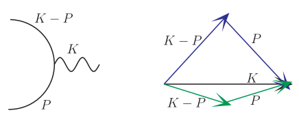
Figure 1: Left: momentum assignments at one of the two current insertions. Right: the 2$\leftrightarrow$2 (blue) and collinear (green) processes are schematically represented.

there are two distinct ways at LO to satisfy momentum conservation. $2\leftrightarrow 2$ processes correspond to the Compton-like and annihilation processes arising from the cuts of the two-loop diagrams obtained by adding an extra gluon, such as the one shown in Fig. 2.

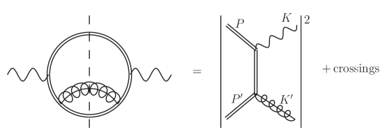
Figure 2: The two-loop diagram on the left corresponds to the square of the amplitude of the diagram on the right and on the squares of its crossing. The interference terms arise from the two-loop diagram where the gluon is exchanged between the two fermionic lines. Double internal lines stand for hard particles, i.e., particles whose momentum is ${\mathcal{O}}(T)$ in at least one component. Plot taken from [19].

Their evaluation boils down schematically to a kinetic-theory picture: an integral over the (Lorentz-invariant) phase space of the matrix elements squared for the processes, folded over the statistical functions $f$ of the medium constituents, i.e.

$$\frac{d\Gamma_{\gamma}}{d^{3}k}\bigg{|}_{2\leftrightarrow 2}\sim\int_{\mathrm{phase\,space}}f(p)f(p^{\prime})(1\pm f(k^{\prime}))\,\left|\mathcal{M}\right|^{2}\delta^{4}(P+P^{\prime}-K-K^{\prime})\,.$$ (4)

The integration over the bare matrix elements encounters the IR divergence of massless Compton scattering. At finite temperature, it is removed by collective plasma excitations. This is implemented by resumming the Hard Thermal Loop (HTL) self-energy [13] in the intermediate quark, rendering the $2\leftrightarrow 2$ processes finite and non-analytic in $g$ through a $\log(g)$ term [14, 15].

Collinear processes, first introduced in [16], contribute at LO. A soft collision with the medium has an order-$\alpha$ chance of inducing the radiation of a collinear photon. Its long formation time can be of the same order of the soft scattering rate, thus causing multiple such scatterings to contribute at the same order and possibly interfere, in what is called the Landau-Pomeranchuk-Migdal (LPM) effect. Its treatment requires the resummation of an infinite number of ladder diagrams [17, 18], as shown in Fig. 3.

$\frac{d\Gamma_{\gamma}}{d^{3}k}\bigg{|}_{\mathrm{coll}}$=

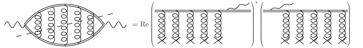
Figure 3: The ladder diagrams that need to be resummed to account for the LPM effect in the collinear region. The cut shown here corresponds to the interference term on the right-hand side. The rungs on the l.h.s. are HTL gluons in the Landau cut. On the r.h.s., the crosses at the lower end of the gluons represent the hard scattering centers, either gluons or fermions. Plot taken from [19].

3 Beyond the LO photon rate: improvements and extensions of pQCD

In this Section we will give an overview of recent results which allow to extend and stretch the pQCD calculation just illustrated. As we mentioned in the introduction, perturbation theory at finite temperature, with its thermal scales and needs for resummations, is properly defined when $g\ll 1$. A next-to-leading order calculation can then be of great help in establishing the reliability of the leading-order rates, which are widely employed in phenomenology. In Sec. 3.1 we will review the recent NLO order calculation of the photon rate [19], whereas in Sec. 3.2 we will present a recent NLO calculation for dileptons [20]. In Sec. 3.3 we will discuss how the LO rates can be generalized to include non-equilibrium viscous effects. Finally, a matrix-model inspired parametrization of the statistical functions close to the critical temperature has been used to compute photon and dilepton rates close to $T_{c}$ and was presented in [21].

3.1 Beyond leading order

It is well known in perturbative thermal field theory that loop corrections involving soft bosons, in our case gluons, are suppressed by a factor of $g$ only. Hence, the NLO correction to the photon rate is just an ${\mathcal{O}}(g)$ correction and schematically it arises from all regions where existing gluons can become soft or extra soft gluons can be added.

One such place is the collinear region. An ${\mathcal{O}}(g)$ correction is given by the NLO contribution to the soft scattering rate and to the jet quenching parameter $\hat{q}$, as computed by Caron-Huot in [22]. In that paper, analyticity properties of retarded amplitudes are used to map the intricate real-time (Minkowskian) four-dimensional calculation of the soft contributions to a much simpler Euclidean three-dimensional problem, basically extending the applicability domain of dimensional reduction from time-independent quantities to the lightcone. This is at the base of the recent lattice studies of $\hat{q}$ [23, 24], presented in [25]. In terms of our calculation, this corresponds to considering the effect of a one-loop rung amid the tree-level ladder of Fig. 3, and similarly of considering the ${\mathcal{O}}(g)$ shift in the thermal mass of the collinear quarks [26].

A new set of processes arises at the next order in the collinear expansion. If at leading order the angle has to be of order $g$, at NLO it can be extended to $\sqrt{g}$, giving rise to semi-collinear processes, where, besides the usual soft spacelike scattering, a soft timelike gluon (a plasmon) can also be absorbed and induce radiation. The evaluation of this region requires a modified version of $\hat{q}$ keeping track of these features. Its relevance for jet energy loss at higher order is being investigated [29].

Finally, we mentioned how at leading order the region where the intermediate quark is soft needs to be treated with care, requiring HTL resummation. At NLO one has the possibility of adding soft gluons to an already soft quarks, giving rise to intricate amplitudes with several HTL propagators and vertices. However, at equilibrium these expressions can be written in terms of retarded functions only and the aforementioned analyticity properties allow a deformation of the integration contour away from the real axis, where the intricacies of HTLs lie, to a region where the amplitudes are much simpler, leading to a compact expression.

In Fig. 4 we plot the rate (in units of the leading-log coefficient) and the ratio of LO+NLO correction over LO rate for $N_{c}=N_{f}=3$ and $\alpha_{\mathrm{s}}=0.3$. Both plots show how in the phenomenologically relevant region the NLO correction represents an ${\mathcal{O}}(20\%)$ increase which comes about from a cancellation between a much larger positive correction from the collinear sector and a negative one from the semi-collinear and soft regions.

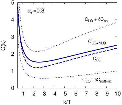
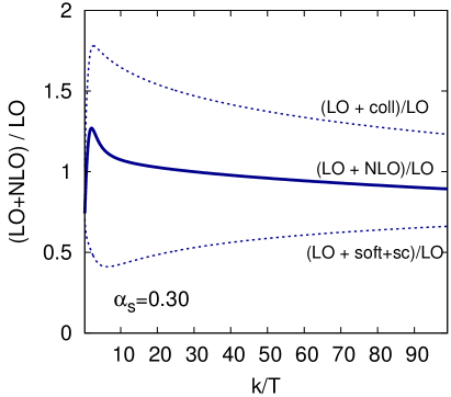
Figure 4: Left: the function, $C(k/T)\equiv d\Gamma/(d^{3}k)(4\alpha_{\rm EM}n_{\!\scriptscriptstyle F}(k)g^{2}T^{2}/(3k))^{-1}$, parametrizing the photon emission rate for $N_{c}=N_{f}=3$ and $\alpha_{\mathrm{s}}=0.3$. The full next-to-leading order function ($C_{{\mathrm{LO}}+{\mathrm{NLO}}}$) is a sum of the leading-order result ($C_{{\mathrm{LO}}}$), a collinear correction ($\delta C_{\rm coll}$), and a soft+semi-collinear correction ($\delta C_{\rm soft+sc}$). The dashed curve labeled $C_{{\mathrm{LO}}}+\delta C_{\rm coll}$ shows the result when only the collinear correction is included, with the analogous notation for the $C_{{\mathrm{LO}}}+\delta C_{\rm soft+sc}$ curve. The difference between the dashed curves provides a uncertainty estimate for the NLO calculation. Right: the ratio between the LO+NLO rate over the LO rate for the same parameters. Plot taken from [19].

This cancellation appears largely accidental, confirmed by the fact that at larger momenta the negative contribution overcomes the positive one. Hence, the band formed by these two curves can be taken as an uncertainty estimate of the LO calculation and should be considered in phenomenological analyses.

3.2 Dileptons

The dilepton invariant mass corresponds to the virtuality of the photon in Eq. (3), $K^{2}>0$. This finite $K^{2}$ now allows a Born term at leading order in the loop expansion, which corresponds to a thermal Drell-Yan process, i.e. the annihilation of a quark-antiquark pair into a virtual photon, as shown on the left of Fig 5.

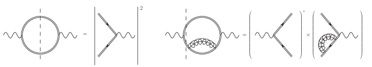
Figure 5: Left: the Born diagram and its cut, corresponding to the thermal Drell-Yan process. Right: a two-loop correction with a cut corresponding to a virtual correction to the Drell-Yan process.

At the next order in the loop expansion one can have both real and virtual corrections to this process. In the former case they correspond to $2\leftrightarrow 2$ processes, as shown in Fig. 2, whereas the latter case is shown on the right in Fig. 5. Cancellations of soft and collinear divergences are at play between these corrections. However, if the frequency and/or the virtuality of the photon become soft, HTL and/or collinear resummations become necessary [30, 31], along the lines of what has been described for the real photon case.

Recently, a complete NLO calculation of the dilepton rate for $K^{2}{\ \lower-1.2pt\vbox{\hbox{\hbox to0.0pt{$>$\hss}\lower 6.0pt\vbox{\hbox{$\sim$}}}}\ }T^{2}$, $k>0$ has been completed in [20]. As the left pane in Fig. 6 shows, the thermal Drell-Yan process (the LO) receives increasingly larger corrections at diminishing $M=\sqrt{K^{2}}$, until the NLO correction overtakes it, signalling the need for resummations. The right pane shows the rate in physical units. For the smallest masses an error band is obtained by varying the renormalization scale for the running coupling by a factor of 2 in each direction.

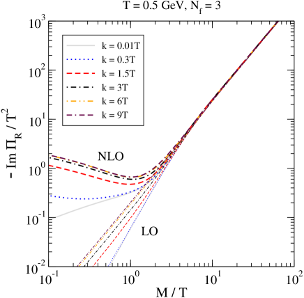
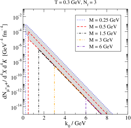
Figure 6: Left: the imaginary part of the retarded polarization, corresponding to the spectral function of the e/m current $J$. Right: the dilepton rate in physical units. Both plots are taken from [20].

A NLO calculation of the dilepton rate for $K^{2}\sim(gT)^{2}$, with HTL and collinear resummations, is underway [33].

3.3 Beyond thermal equilibrium

As we mentioned, the medium produced in heavy-ion collisions undergoes a viscous hydrodynamic evolution. Assessing thus the importance of the deviation from equilibrium is of great relevance for a quantitative description of photon flow data, such as the “$v_{2}$ puzzle” widely reported at this conference. To this end, $2\leftrightarrow 2$ processes have been computed in an off-equilibrium setting [34], as reported in [35]. The simple kinetic picture of Eq. (4) can be readily generalized, by replacing the equilibrium distributions $f$ with first-order perturbed ones which depend on the anisotropic tensor $\pi^{\mu\nu}$. In the soft region, equilibrium Hard Thermal Loops are replaced by off-equilibrium Hard Loops. We refer to [35] for the phenomenological implications; from a theoretical standpoint, we remark that it would be very interesting to see an anisotropic extension of collinear processes, which could be more intricate due to the instabilities of gluonic Hard Loops [36, 37].

4 Lattice

As we mentioned in the introduction, a direct determination of Eq. (3) is hampered by its Minkowskian nature. The corresponding Euclidean correlator, accessible by lattice methods, is

$$W_{E}(\tau,{\bf{k}})\equiv\int d^{3}x\left\langle J_{\mu}(\tau,\mathbf{x})J_{\mu}(0)\right\rangle e^{i{\bf{k}}\cdot\mathbf{x}}\,.$$ (5)

This Euclidean correlator is related by analytical continuation to the Minkowskian one: $W_{E}(\tau,{\bf{k}})=W^{<}(i\tau,{\bf{k}})$, which allows to write the former in terms of the electromagnetic spectral function as

$$W_{E}(\tau,{\bf{k}})=\int_{0}^{\infty}\frac{dk^{0}}{2\pi}\rho_{J}(k^{0},{\bf{k}})\frac{\cosh\left(k^{0}(\tau-1/(2T))\right)}{\sinh\left(\frac{k^{0}}{2T}\right)}.$$ (6)

One is then faced with the numerical inversion of the r.h.s of Eq. (6), starting from a discrete set of points with errorbars on the l.h.s. At vanishing momentum ($k=0$) the inversion has been performed using Bayesian MEM techniques or fitting Ansätze (see [38, 39] for recent results). The $k=0$ spectral function encodes the physics of electric conductivity in the transport peak at the origin and the dilepton rate for finite $k^{0}$. The obtained result shows a similar trend to the resummed HTL calculation of [30] and at large values of the virtuality is well described by the perturbative Born term.

At non-vanishing momentum, $k>0$, the spectral function describes the physics of spacelike scattering with medium constituents ($0<k^{0}<k$), real photon production ($k^{0}=k$) and dilepton production ($k^{0}>k$). Although a determination of $W_{E}$ for $k>0$ exists [39], no attempt at spectral function reconstruction has been performed so far. It is however straightforward to use Eq. (6) directly, i.e. to obtain $W_{E}$ from a perturbative determination of the spectral function, as carried out in [20]. The leading-order spectral function (complemented with higher-order vacuum contributions) is shown to be in qualitative agreement with the lattice data. It is to be remarked, however, that extremely interesting features, such as the real photon contribution $k^{0}=k$, vanish in the LO spectral function. In more detail, Fig. 7 shows the bare spectral function (without any higher-order vacuum contributions), normalized by the frequency, with superimposed dashed lines for the ratio of hyperbolic functions in Eq. (6) (multiplied by frequency) for different values of $\tau$. It is the overlap of these curves that determines the Euclidean correlator and, as the figure shows, it is dominated by the approximate linear rise of the dilepton ($k^{0}>k$) part of the spectral function. Fig. 8 shows the comparison [20] of the perturbative [20] and lattice calculations [39] in the longitudinal (left) and transverse (right) channels. We refer to [20] for a discussion on the caveats of this comparison.

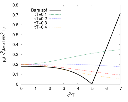
Figure 7: The Born spectral function ($g=0$) in black, for $k=5T$, divided by the frequency. The superimposed dashed lines are $k^{0}\,\cosh\left(k^{0}(\tau-1/(2T))\right)/\sinh\left(\frac{k^{0}}{2T}\right)$ for different values of $\tau$.

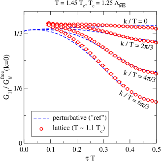
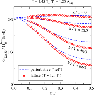
Figure 8: The left and right panes show the comparison of the perturbative and lattice data, as explained in the main text. Both are taken from [20].

5 Summary and conclusions

The knowledge of the production rates and of the associated theoretical uncertainty is an essential ingredient for the phenomenological description of electromagnetic hard probes. In this contribution we have illustrated the basics of the calculation of the LO pQCD rates, widely employed in phenomenology. These calculations often require the inclusion of physically distinct processes and careful resummations of soft and collinear physics. The reliability of these LO rates can be tested through NLO calculations. These indeed provide a first estimate of the theory error budget for photons [19] and large-mass dileptons [20]. As a byproduct, technological advancements have been obtained in the form of factorizations, sum rules for Hard Thermal Loop and calculations of spectral functions [40, 41] that are employable in other domains, such as jet propagation and quenching.

For what concerns the lattice, we have reviewed the difficulties in the extraction of the spectral function. Recent results [38, 39] are available for $k=0$ and a first comparison with perturbation theory was performed, for $k\neq 0$, at the Euclidean correlator level [20]. Furthermore, important ingredients for the perturbative calculations, such as the soft scattering rate, are now being determined non-perturbatively on the lattice [23], opening the way for possible future “hybrid” calculations, where non-perturbative inputs are used in perturbative calculations.

Acknowledgements This work was supported by the Institute for Particle Physics (Canada) and the Natural Sciences and Engineering Research Council (NSERC) of Canada. I would like to acknowledge the Mainz Institute for Theoretical Physics (MITP) for enabling me to complete a portion of this work.

References

- [1] L. Ruan, these proceedings, arXiv:1407.8153.
- [2] H. Niemi, these proceedings.
- [3] E. Bratkovskaya, these proceedings.
- [4] M. L. Bellac, Cambridge University Press, 1996.
- [5] J. M. Maldacena, Adv.Theor.Math.Phys. 2 (1998) 231–252. arXiv:hep-th/9711200.
- [6] E. Witten, Adv.Theor.Math.Phys. 2 (1998) 253–291. arXiv:hep-th/9802150.
- [7] S. Gubser, I. R. Klebanov, A. M. Polyakov, Phys.Lett. B428 (1998) 105–114. arXiv:hep-th/9802109.
- [8] S. Caron-Huot, P. Kovtun, G. D. Moore, A. Starinets, L. G. Yaffe, JHEP 0612 (2006) 015. arXiv:hep-th/0607237.
- [9] B. Hassanain, M. Schvellinger, JHEP 1212 (2012) 095. arXiv:1209.0427.
- [10] R. Baier, S. A. Stricker, O. Taanila, A. Vuorinen, JHEP 1207 (2012) 094. arXiv:1205.2998.
- [11] R. Baier, S. A. Stricker, O. Taanila, A. Vuorinen, Phys.Rev. D86 (2012) 081901. arXiv:1207.1116.
- [12] D. Steineder, S. A. Stricker, A. Vuorinen, JHEP 1307 (2013) 014. arXiv:1304.3404.
- [13] E. Braaten, R. D. Pisarski, Nucl.Phys. B337 (1990) 569.
- [14] J. I. Kapusta, P. Lichard, D. Seibert, Phys.Rev. D44 (1991) 2774–2788.
- [15] R. Baier, H. Nakkagawa, A. Niegawa, K. Redlich, Z.Phys. C53 (1992) 433–438.
- [16] P. Aurenche, F. Gelis, R. Kobes, H. Zaraket, Phys.Rev. D58 (1998) 085003. arXiv:hep-ph/9804224.
- [17] P. B. Arnold, G. D. Moore, L. G. Yaffe, JHEP 0111 (2001) 057. arXiv:hep-ph/0109064.
- [18] P. B. Arnold, G. D. Moore, L. G. Yaffe, JHEP 0112 (2001) 009. arXiv:hep-ph/0111107.
- [19] J. Ghiglieri, J. Hong, A. Kurkela, E. Lu, G. D. Moore, D. Teaney, JHEP 1305 (2013) 010. arXiv:1302.5970.
- [20] M. Laine, JHEP 1311 (2013) 120. arXiv:1310.0164.
- [21] S. Lin, these proceedings.
- [22] S. Caron-Huot, Phys.Rev. D79 (2009) 065039. arXiv:0811.1603.
- [23] M. Panero, K. Rummukainen, A. Schäfer, Phys.Rev.Lett. 112 (2014) 162001. arXiv:1307.5850.
- [24] M. Laine, A. Rothkopf, JHEP 1307 (2013) 082. arXiv:1304.4443.
- [25] M. Panero, these proceedings.
- [26] S. Caron-Huot, Phys.Rev. D79 (2009) 125002. arXiv:0808.0155.
- [27] B. Brandt, A. Francis, M. Laine, H. Meyer, JHEP 1405 (2014) 117. arXiv:1404.2404.
- [28] H. Meyer, these proceedings.
- [29] J. Ghiglieri, G. D. Moore, D. Teaney, in preparation.
- [30] E. Braaten, R. D. Pisarski, T.-C. Yuan, Phys.Rev.Lett. 64 (1990) 2242.
- [31] P. Aurenche, F. Gelis, G. Moore, H. Zaraket, JHEP 0212 (2002) 006. arXiv:hep-ph/0211036.
- [32] I. Ghisoiu, M. Laine, arXiv:1407.7955.
- [33] J. Ghiglieri, et al., in preparation.
- [34] C. Shen, U. W. Heinz, J.-F. Paquet, I. Kozlov, C. Gale, arXiv:1308.2111.
- [35] C. Shen, U. Heinz, J.-F. Paquet, C. GalearXiv:1403.7558.
- [36] P. Romatschke, M. Strickland, Phys.Rev. D68 (2003) 036004. arXiv:hep-ph/0304092.
- [37] P. B. Arnold, J. Lenaghan, G. D. Moore, JHEP 0308 (2003) 002. arXiv:hep-ph/0307325.
- [38] H.-T. Ding, A. Francis, O. Kaczmarek, F. Karsch, E. Laermann, et al., Phys.Rev. D83 (2011) 034504. arXiv:1012.4963.
- [39] O. Kaczmarek, E. Laermann, M. Müller, F. Karsch, H. Ding, et al., PoS ConfinementX (2012) 185. arXiv:1301.7436.
- [40] M. Laine, JHEP 1305 (2013) 083. arXiv:1304.0202.
- [41] M. Laine, JHEP 1308 (2013) 138. arXiv:1307.4909.