A covariantly foliated higher dimensional space-time: Implications for short distance gravity and BSM physics

Abstract

We consider the space-time at short distances in which it is described by a $D$-dimensional manifold (bulk) carrying out the principal bundle structure. As a result, this space-time manifold is foliated in the covariant way by the $(D-4)$-dimensional submanifolds, realized as the space-like internal spaces, that are smooth copies of the Lie group $G$ considered in this paper as the special unitary group. The submanifolds being transversal to the internal spaces are realized as the external spaces and in fact identified as the usual $4$-dimensional world. The fundamental degrees of freedom determining the geometrical dynamics of the bulk corresponding with short distance gravity are given by the gauge fields, the external metric field and the modulus fields setting dynamically the volume of the internal spaces. These gauge fields laying the bulk is to point precisely out the local directions of the external spaces which depend on the topological non-triviality of the space-time principal bundle. The physical size of the internal spaces is fixed dynamically by the moduli stabilization potential which completely arise from the intrinsic geometry of the bulk. A detail description of the low energy bulk gravity in the weak field limit is given around the classical ground state of the bulk. Additionally, we investigate the dynamics of the fundamentally $4$-dimensional Weyl spinor fields and the fields of carrying out the non-trivial representations of the Lie group $G$ propagating in the bulk in a detail study. These results suggest naturally the possible solutions to some the experimental problems of Standard Model, the smallness of the observed neutrino masses and a dark matter candidate.

I Introduction and Proposal

Our present understanding of the observable space-time experimentally confirmed being valid to distances of the order $10^{-16}$ cm is well provided by General Relativity (GR) of the gravity. However, the gravitational phenomena only play the important roles in the macroscopic world whereas in the quantum world of the elementary particles they are not very significant due to the gravitational coupling constant which is so small compared those in Standard Model (SM). As well-known, all nongravitational interactions are described by theory of connections (or gauge fields) which are accommodated into the quantum framework. This situation is completely different to that for the gravitational interaction. Since it is possible that unknown high energy gravitational effects should be contained in the mysteriously deeper structures of the space-time. It should be emphasized that the motivation for seeking of high energy gravitational effects is also come from some other significant reasons, such as physical phenomena associated with gravitational collapse. These imply that the space-time at high energy regions or short distances may in fact have dimensionality of more than four as well as possess rather complex topologies and geometrical structures.

The multidimensional universe possibility was first proposed by Kaluza and Klein in attempting to unify the electromagnetic interaction and the gravity in a $5$-dimensional space-time. The extension tried to unify the forces of SM to the gravity can see in Witten1981 ; Bailin-Love1987 . However, it is very interesting in recent years that the physical models based on extra-dimensions have devoted enormously to solve problems in particle physics as well as cosmology Antoniadis90 ; ADDmodel ; RSImodel ; UEDmodel . The higher dimensional extension of the space-time can thus offer a new way of looking for Beyond the Standard Model (BSM) physics. It should be noted that the dimensional reduction of the previously most higher dimensional scenarios explicitly breaks the higher dimensional covariance and the higher dimensional Poincaré symmetry, for example, via the presence of $3-$brane as

$$\mathbb{R}^{1,D-1}\times SO(D-1,1)\longrightarrow\mathbb{R}^{1,3}\times SO(3,1)\times SO(D-4),$$ (1)

where two first factors corresponds to translational symmetries and the Lorentz group along the $3$-brane, and the second one does to the rotation group along ($D-4$) extra dimensions which are transverse to $3$-brane. Furthermore, a natural physical mechanism to compact the extra dimensions and stabilize the corresponding volume modulus fields is obviously still undetermined so far.

In this work, we consider a braneless higher dimensional space-time $B^{D}$ of $D$-dimensions which is assumed a principal bundle MDGfP ; Nakahara . It is in general factorized locally as the topology product of two spaces, $U\times G$. Here $U$ is an open subset of $4$-dimensional pseudo-Riemannian manifold $M^{4}$ with the Lorentz metric, and $G$ is a Lie group which we restrict our attention to the special unitary group. Therefore, there exists a diffeomorphism map $f$ smoothly deforming $U\times G$ to a local neighbourhood $\pi^{-1}(U)\subset B^{D}$, which is constructed as an inverse image of the surjective projection

$$\pi:B^{D}\longrightarrow M^{4},$$ (2)

as follows

$$f:U\times G\longrightarrow\pi^{-1}(U),$$ (3)

which is also called a local trivialization. Through such diffeomorphic maps, it is quite clear to see that a set of points belonging $B^{D}$ which corresponds with an inverse image $\pi^{-1}(x)$ ($x\in M^{4}$), called the fibre at $x$, forms a submanifold of $B^{D}$ that is a smooth copy of the Lie group $G$. All such submanifolds are not necessary as $G$ and obviously disjoint with together. Since the underline geometry of $B^{D}$ is always given as the $D$-dimensional manifold foliated by ($D-4$)-dimensional submanifolds of which are smoothly equivalent to the Lie group $G$. It is important that this foliation is exactly to remain the higher dimensional covariance and symmetries. These submanifolds will be realized as the space-like internal spaces and also called the leaves of the foliation Benjacu2006 . As indicated above, one can easily see that at starting point we consider the internal spaces to be compact in the sense of the mathematics. It is also important that four-dimensional submanifolds whose vector fields point from one fibre to another, thus being transversal to the internal spaces, will be in fact identified as the usual four-dimensional world. They are called the external spaces and in general locally smooth equivalence to $M^{4}$. This means that the dynamics of the fields in $B^{D}$ should correspond with the propagation along the internal spaces and external spaces. However, in low energy limit we only observe the motion from an internal space to another leading to the dimensional reduction that is very natural to produce the usual four-dimensional world as will be shown in this paper. Effects of the dynamics along the internal spaces and others coming from extra dimensions are elegantly hidden from the present experiments on particle accelerators, astrophysics and cosmology.

Through the local description (3), coordinates of a point on $B^{D}$ are given as

$$X^{M}=x^{\mu},\hskip 14.22636ptM=0,1,2,3,$$

$$X^{M}=\frac{\theta^{a}}{\Lambda}\equiv\hat{\theta}^{a}.\hskip 14.22636ptM=4,...,D-1.$$ (4)

Here $\{x^{\mu}\}\in\mathbb{R}^{4}$, and a set of real numbers $\{\theta^{a}\}$ parameterizes each element of the Lie group G as, $g=\textrm{exp}\{i\theta^{a}T_{a}\}$, with the generators $T_{a}$ ($a=1,...,D-4$) satisfying the following commutation relation of the Lie algebra $\mathfrak{g}$ of the Lie group $G$

$$[T_{a},T_{b}]=if^{c}_{ab}T_{c},$$ (5)

where $f^{c}_{ab}$ are the structure constants. The coordinates $x^{\mu}$ are realized as the $4$-dimensional external coordinates while $\theta^{a}$ (or $\hat{\theta}^{a}$ ) are realized as the internal coordinates, or fibre ones, which offer obviously the global coordinate system on each internal space. It should be noted that due to $\theta^{a}$ being dimensionless a new energy scale $\Lambda$ characterizing physically to the internal spaces is taken in the natural way. It should be noted that this scale is not realized as the inverse radius of the compact internal spaces which is in fact determined only if their metric is endowed. This energy scale will be responsible for exciting the physical states coming from the extra dimensions. Since it should be high enough.

The rule of the local coordinate transformations which corresponds with a non-empty overlap of two any local neighbourhoods is defined by

$$x^{\prime\mu}=\Lambda(x){{}^{\mu}}_{\nu}x^{\nu},\ e^{i\theta^{\prime a}T_{a}}=h(x)e^{i\theta^{a}T_{a}},$$ (6)

where $\Lambda(x)$ and $h(x)=\exp\{i\alpha^{a}(x)T_{a}\}$ are elements of the linear transformation group $GL(4,\mathbb{R})$ and the Lie group $G$, respectively. Notice that, the rule of internal coordinate transformation can be easily derived from (3). As a general principle, the invariant principle of the physical laws requires that higher dimensional physical quantities have to be covariant under the local coordinate transformations above.

This paper is organized as follows. In Sec. II, we present essential settings of the proposed space-time. We study the classical dynamics of pure bulk gravity in Sec. III. In Sec. IV, the classical ground state of the bulk space-time is determined, and the perturbative description of the bulk gravity in the low energy limit is investigated around this background. In Sec. V, we show how the $4$-dimensional Weyl spinor fields occur naturally on $B^{D}$, and their dynamical Lagrangian is constructed in a consistent way. As a result, we provide a understanding for the natural smallness origin of the observed neutrino masses. In Sec. VI, the dynamics of the fields of carrying out the local non-trivial representations of the Lie group $G$ is considered. Such a field is possible to suggest a dark matter candidate. Finally, we devote to conclusions and comments in the last section, Sec. VII.

II Settings of Space-time $B^{D}$

II.1 The gauge fields of the space-time $B^{D}$

Each local coordinate system on $B^{D}$ given above induces naturally the basic vectors for the tangent spaces of $B^{D}$ presented by

$$\{\partial_{M}\}=\left(\{\partial_{\mu}\},\{\Lambda\partial_{a}\equiv\hat{\partial}_{a}\}\right),$$ (8)

which rotate under the local coordinate transformations (6) as follows

$$\partial_{\mu} \longrightarrow \partial^{\prime}_{\mu}=\frac{\partial x^{\nu}}{\partial x^{\prime\mu}}\partial_{\nu}+\frac{\partial\hat{\theta}^{a}}{\partial x^{\prime\mu}}\hat{\partial}_{a},$$

$$\hat{\partial}_{a} \longrightarrow \hat{\partial}^{\prime}_{a}=\frac{\partial\hat{\theta}^{b}}{\partial\hat{\theta}^{\prime a}}\hat{\partial}_{b}.$$ (9)

With respect to $B^{D}$, each tangent space $T_{X}B^{D}$ at a given point on it is always split into the following form

$$T_{X}B^{D}=H_{X}B^{D}\oplus V_{X}B^{D},$$ (10)

where $V_{X}B^{D}$ is called the vertical tangent subspace which is tangent to an internal space whereas its complement, $H_{X}B^{D}$, is called the horizontal tangent subspace which is tangent to an external space. It is direct to see that vectors $\hat{\partial}_{a}$ transform in the covariant way under the rule of the fibre coordinate transformation. This means that the total of $\{\hat{\partial}_{a}\}$ under the compatibility condition corresponding to the second transformation of (9) are equally good. Since they provide the well-defined local bases for all vertical tangent spaces. On the other hand, the directions along the internal spaces are defined independently of choosing a local basis. However, the well-defined local bases for all horizontal tangent spaces are not specified as seen more clearly from the transformation in the first line of (9). This is as a result of that the directions to be transversal to the fibres depend on the information of topological non-triviality, or twisting, of the bundle $B^{D}$.

The principled way of how to move from an internal space to another is given via the presence of a $\mathfrak{g}$-valued one-form connection $\omega(X)$ which annihilates the horizontal vectors. It is explicitly written in a local neighbourhood $\pi^{-1}(U)$ as follows

$$\omega(X)=g^{-1}i\pi^{*}A(x)g+g^{-1}dg=ig^{-1}T_{a}g[d\theta^{a}+g_{\textrm{i}}A^{a}_{\mu}(x)dx^{\mu}],$$ (11)

where $g=e^{i\theta^{a}T_{a}}$, $d$ is the exterior differential operator, the pullback map $\pi^{*}$ is induced by the projection operator $\pi$, $A^{a}_{\mu}$ with the dimension $[A^{a}_{\mu}]=1$ are the gauge fields, and $g_{\textrm{i}}$ is a dimensionless constant (it will play the role of the gauge coupling constant characterizing the strength of the interaction mediated by the $A^{a}_{\mu}$). Because of the pullback map $\pi^{*}$ acting on the local one-form $A(x)=g_{\textrm{i}}A^{a}_{\mu}(x)T_{a}dx^{\mu}$ lying on $M^{4}$, the gauge fields $A^{a}_{\mu}$ in the last expression in Eq. (11) thus live on $B^{D}$ in which they define topological non-triviality of the space-time $B^{D}$ through their curvature tensor as indicated below. The reader should not confuse $A^{a}_{\mu}$ in this framework with the gauge fields in the usual gauge theories at which they live on $M^{4}$ (in this case the space-time) Daniel-Viallet1980 . Any curve, $\overline{\gamma}(t)=(x^{\mu}(t),\hat{\theta}^{a}(t))$, flows transversely to the fibres then each its tangent vector $V(t)$ is horizontal one and thus is annihilated by the connection. Since we can get the following relation

$$\frac{dg(t)}{dt}=-ig_{\textrm{i}}A^{a}_{\mu}T_{a}\frac{dx^{\mu}(t)}{dt}g(t),$$ (12)

where $g(t)=e^{i\theta^{a}(t)T_{a}}$. Then, we find

$$\frac{d\theta^{a}(t)}{dt}=-g_{\textrm{i}}A^{a}_{\mu}\frac{dx^{\mu}(t)}{dt},$$ (13)

that results in the formal expression for $V(t)$ as

$$V(t) = \frac{dx^{\mu}(t)}{dt}\partial_{\mu}+\frac{d\hat{\theta}^{a}(t)}{dt}\hat{\partial}_{a}$$ (14)

$$= \frac{dx^{\mu}(t)}{dt}(\partial_{\mu}-g_{\textrm{i}}A^{a}_{\mu}\partial_{a})\equiv\frac{dx^{\mu}(t)}{dt}\hat{\partial}_{\mu}.$$

The total of $\{\hat{\partial}_{\mu}\}$ provide the well-defined local bases for whole horizontal tangent spaces on $B^{D}$ if the gauge fields $A^{a}_{\mu}$ transform as

$$A^{\prime}_{\mu}(x^{\prime})=\frac{\partial x^{\nu}}{\partial x^{\prime\mu}}\left[h(x)A_{\nu}(x)h(x)^{-1}+\frac{1}{ig_{\textrm{i}}}h(x)\partial_{\nu}h(x)^{-1}\right],$$ (15)

where $h(x)$ is given in (6), and $A_{\mu}=A^{a}_{\mu}T_{a}$. This transformation is to correspond with that the connection taken in two different local neighbourhoods coincides together in an intersection region. We can see that the transformation rule (15) is to combine of both the $4$-dimensional external coordinate and the usual gauge transformations. This is due to that it has an origin from the local coordinate transformations of the higher dimensional space-time. It can be verified that an infinitesimal variation of $A^{a}_{\mu}$ is taken as

$$\delta A^{a}_{\mu}(x)=-\partial_{\mu}\epsilon^{\nu}(x)A^{a}_{\nu}(x)-\epsilon^{\nu}(x)\partial_{\nu}A^{a}_{\mu}(x)+f^{a}_{bc}\alpha^{b}(x)A^{c}_{\mu}(x)-\partial_{\mu}\alpha^{a}(x),$$ (16)

where infinitesimal parameters $\epsilon^{\mu}(x)$ and $\alpha^{a}(x)$ are defined as, $x^{\prime\mu}=x^{\mu}+\epsilon^{\mu}(x)$ and $\textrm{exp}\{i\alpha^{a}(x)T_{a}\}\cong 1+i\alpha^{a}(x)T_{a}$, respectively. The first two terms in Eq. (16) come from the infinitesimal transformation of the $4$-dimensional external coordinates while the remaining ones present the usually infinitesimal gauge transformation.

We have seen that the gauge fields $A^{a}_{\mu}$ gives the covariant way to determine the directions of the usual $4$-dimensional world in $B^{D}$. Since an arbitrary particle moving along the $4$-dimensional external directions of the bulk may be coupled with $A^{a}_{\mu}$. This is easily seen by the appearance of the gauge fields $A^{a}_{\mu}$ in the derivatives $\hat{\partial}_{\mu}$ implying that the field propagating in the bulk having non-zero derivatives in the internal variables would interact to $A^{a}_{\mu}$. It is interesting to interpret that corresponding gauge charges are generated dynamically through the physical kinetics in the internal spaces. This means that such interaction is of the manifestation of properties of the internal dynamics. In addition to such coupling perspective, there will be known the coupling occurring in the context of the usual gauge theory in which the gauge fields $A^{a}_{\mu}$ are coupled to the fields of carrying out non-trivial representations of the group $G$, as we will discuss in Sec. VI. Eventually, the connection one-form is realized as the elegant object in the mathematical point of view while the gauge fields $A^{a}_{\mu}$ carry out the interesting physical significance as force-carrying particles.

Any vector field $V(X)$ on $B^{D}$ is always written in external and internal components in the following form

$$V(X)=V^{\mu}_{H}(X)\hat{\partial}_{\mu}+V^{a}_{V}(X)\hat{\partial}_{a}.$$ (17)

Since $V^{\mu}_{H}(X)$ and $V^{a}_{V}(X)$ do not mix with each other, they are thought of as the independently physical fields at the fundamentally higher dimensional level. It is also straightforward to generalize that for a general tensor field on the bulk in which there will have additionally hybrid fields including both the external and internal indices.

A better understanding about the topological non-triviality of the bundle $B^{D}$ is given through a curvature two-form $\Omega$ of the given connection. The curvature would tell us how to distinguish a given connections on $B^{D}$ that is sufficiently different to the flat connection in which its curvature vanishes to correspond with the trivial bundle $B^{D}$. This means that it measures the twisting of the bundle $B^{D}$. The curvature is defined by the Cartan’s structure equation as

$$\Omega=d\omega+\omega\wedge\omega,$$ (18)

where $\wedge$ is the wedge product on the space of the differential forms living the bulk. From this definition, one can show that $\Omega$ acts on any pair of horizontal vectors to yield an element of $\mathfrak{g}$ but vanishing for the remaining cases. In other works, only the horizontal components of the curvature are not zero in which they are defined explicitly as follows

$$\Omega_{\mu\nu}(X)=ig_{\textrm{i}}e^{-i\theta}F_{\mu\nu}(x)e^{i\theta},$$ (19)

where

$$F_{\mu\nu}(x)=\left(\partial_{\mu}A^{a}_{\nu}-\partial_{\nu}A^{a}_{\mu}-g_{\textrm{i}}f^{a}_{bc}A^{b}_{\mu}A^{c}_{\nu}\right)T_{a},$$ (20)

is well-known as the Yang-Mills field strength tensor. In an overlap region between any two neighbourhoods, the curvature $\Omega$ has to obey, $\Omega=\Omega^{\prime}$, leading to the rule of the gauge transformation for $F_{\mu\nu}$ as follows

$$F^{\prime}_{\mu\nu}(x^{\prime})=\frac{\partial x^{\rho}}{\partial x^{\prime\mu}}\frac{\partial x^{\lambda}}{\partial x^{\prime\nu}}h(x)F_{\rho\lambda}(x)h^{-1}(x),$$ (21)

where $h(x)$ is given in (6).

II.2 Global frame of the vertical tangent spaces

The Lie group $G$ acts smoothly and freely on $B^{D}$ as the active diffeomorphism transformations, known as the right action, to induce naturally so-called fundamental vector fields which are defined globally on it. All of them form a vector space preserving the structure of the Lie algebra $\mathfrak{g}$, thus, it is isomorphic to $\mathfrak{g}$. The basic vector fields of this vector space denoted by $K_{i}(X)$ $(\equiv\hat{\partial}_{i})$, with $i=1,2,...,D-4$, satisfy the following Lie bracket

$$[K_{i}(X),K_{j}(X)]=\overline{f}^{k}_{ij}K_{k}(X),$$ (23)

where $\overline{f}^{k}_{ij}=\Lambda f^{k}_{ij}$ are the corresponding structure constants. These structure constants can also realized as a tensor of type $(1,2)$ transforming under the global rotation of the frame fields $K_{i}$ read

$$K_{i}(X)\longrightarrow K^{\prime}_{i}(X)={A_{i}}^{j}K_{j}(X),$$ (24)

where ${A_{i}}^{j}$ is in general a constant matrix of the general linear group $GL(D-4,\mathbb{R})$. We should note that each vertical tangent space is also isomorphic to $\mathfrak{g}$ due to that the internal spaces are to deform smoothly of $G$. It is thus very important that $\{K_{i}\}$ constitutes a global frame for the whole vertical tangent spaces on $B^{D}$.

These frame fields are written explicitly in a local neighbourhood as

$$K_{i}(X)={K_{i}}^{a}(X)\hat{\partial}_{a}.$$ (25)

Here ${K_{i}}^{a}(X)$ is dimensionless and transforms as a covector under the rule of the fibre coordinate transformation and as a vector under the transformation (24). The fact that a horizontal vector field is transported along a flow generated by a fundamental vector field remains again another one. On the other hand, we must impose a condition on the following Lie derivatives, $[V_{H},K_{i}(X)]\in H_{X}B^{D}$ for all of $i=1,...,D-4$, with $V_{H}$ to be a horizontal vector field. Thus, this results in the equations for ${K_{i}}^{a}(X)$ as

$$\left(\partial_{\mu}-g_{\textrm{i}}A^{b}_{\mu}\partial_{b}\right){K_{i}}^{a}(X)=0.$$ (26)

These first-order partial differential equations may be considered as the equations describing the evolution of the frame fields $K_{i}(X)$ under the dynamics of the bulk space-time. It is important to be emphasized that these equations are properly defined in a pure mathematical way rather than from the equations of motion obtained by varying the corresponding action. This means that the fields $K_{i}(X)$ would be not realized as the physical degrees of freedom in the usual sense, but are the mathematically axial fields.

The fundamental vector fields are used to describe the infinitesimal displacement behaviour of the action of the Lie group $G$ on $B^{D}$. It is expressed in terms of parameters of the infinitesimal transformation $\varepsilon^{i}$ as

$$x^{\prime\mu}=x^{\mu},\hskip 28.45274pt\theta^{\prime a}=\theta^{a}+\varepsilon^{i}{K_{i}}^{a}.$$ (27)

The flows of $K_{i}(X)$ running along the internal spaces lead to the infinitesimal displacements obviously only performed along these spaces. Since the $4$-dimensional external coordinates in the same local neighbourhood do not change. Notice also that, $\varepsilon^{i}$ are independent on the bulk coordinates because the action of the Lie group $G$ is defined globally. The second equation of Eq. (27) suggests that $K_{i}(X)$ play the role of the infinitesimal generators corresponding with the active diffeomorphism transformations resulting from the action of $G$ on the bulk. With respect a physical field $\psi$ which is an active diffeomorphism invariance under the action of $G$, then Lie derivatives of $\psi$ along all fields $K_{i}$ vanish

$$\mathcal{L}_{K_{i}}\psi=0.$$ (28)

Here the Lie derivatives are defined for general mathematical objects rather than only the usual tensor fields on $B^{D}$. The vector fields are characterized by Eq. (28) to point out the symmetric directions with resepct to the field $\psi$ in the internal spaces. In this case, the internal dynamics of $\psi$ is governed by the intrinsic symmetry nature under $G$ rather than by the sources. As indicated in the paper Gaul-Rovelli2000 , the active diffeomorphism invariance is a property of the dynamical theory itself whereas the passive diffeomorphism invariance is a property of the formulation of a dynamical theory. A specially interesting case in which the right-hand of Eq. (28) is not vanished but is proportion to $\psi$ will lead to the conformal diffeomorphism invariance for $\psi$ under $G$.

Let us introduce dual fields of $K_{i}(X)$, denoted by $K^{i}(X)$, satisfying the following conditions

$$\langle K^{i},K_{j}\rangle=\delta^{i}_{j},$$ (29)

which form a global basis for the internal one-form fields on $B^{D}$. Their local form is taken as

$$K^{i}(X)={K^{i}}_{a}(X)\left(d\hat{\theta}^{a}+\frac{g_{\textrm{i}}A^{a}_{\mu}dx^{\mu}}{\Lambda}\right),$$ (30)

where ${K^{i}}_{a}(X)$ transform as an vector under the rule of the fibre coordinate transformation and as covector under the rotation of $K_{i}$ given in (24). With the help of both (23) and (26) equations, it can be easily verified that $K^{i}(X)$ obey the equations extended from the usual Maurer-Cartan’s structure equations as follows

$$dK^{i}=-\frac{1}{2}\overline{f}^{i}_{jk}K^{j}\wedge K^{k}+\frac{g_{\textrm{i}}}{2\Lambda}F^{i}_{\mu\nu}dx^{\mu}\wedge dx^{\nu},$$ (31)

where $F^{i}_{\mu\nu}$ is defined in terms of $A^{i}_{\mu}={K^{i}}_{a}A^{a}_{\mu}$ of the following form

$$F^{i}_{\mu\nu}=\partial_{\mu}A^{i}_{\nu}-\partial_{\nu}A^{i}_{\mu}+g_{\textrm{i}}f^{i}_{jk}A^{j}_{\mu}A^{k}_{\nu}.$$ (32)

The mathematical interpretation of $F^{i}_{\mu\nu}$ is to measure the failure of integrability of the horizontal distribution because the Lie bracket of any two horizontal frame fields is given as

$$[\hat{\partial}_{\mu},\hat{\partial_{\nu}}]=-\frac{g_{\textrm{i}}}{\Lambda}F^{i}_{\mu\nu}K_{i},$$ (33)

which leads to a vertical vector. Because of that the bundle $B^{D}$ is topologically non-trivial, the external submanifolds are in general joint together. In the case of all the components $F^{i}_{\mu\nu}$ vanishing, the horizontal distribution is integrable since by the Frobenius s theorem the higher dimensional space-time $B^{D}$ is also foliated by the $4$-dimensional external submanifolds.

III Bulk Gravity

In the minimal formalism, the fundamental variables describing the dynamics of the gravity consist of the gauge fields $A^{a}_{\mu}$ together with the geometrical field (a bulk metric tensor) determining the smooth of the bulk manifold as well as a causal structure between the physical events. An ansatz for the bulk metric is given locally in the most general form as follows

$$ds^{2}_{B}=g_{\mu\nu}(X)dx^{\mu}dx^{\nu}-\gamma_{ij}(X)K^{i}K^{j},$$ (34)

which describes two separately infinitesimal invariant intervals on the external and internal spaces, respectively. The signature of the metric $g_{\mu\nu}$ is chosen as, $(+---)$, since the sign “$-$” in the second term of Eq. (34) refers the space-like nature of the internal spaces. In this way, $\gamma_{ij}$ includes obviously global degrees of freedom due to the internal coframe fields $K^{i}$ defined globally on the bulk. It can thus be interpreted in sense of the volume modulus fields which set dynamically the size of the internal spaces. Under this description, all of them are manifestly independent with each other. Since they are realized as the fundamental fields unified in the same non-trivial geometrical structure of the higher dimensional space-time. In addition to the fields created the bulk gravity, we also have the mathematically axial field ${K_{i}}^{a}$, or its dual ${K^{i}}_{a}$.

It is interesting that the internal metric $\gamma_{ij}$ enjoys naturally an important one which it is a constant matrix with respect the coframe fields $K^{i}$. In this case, one may choose others so that $\gamma_{ij}$ would be diagonal. It thus leads to the metric $\gamma_{ij}$ that may be expressed as follows

$$\gamma_{ij}=v_{i}\delta_{ij},$$ (35)

where $v_{i}$ are all positive constants, and $\delta_{ij}$ is the Kronecker delta function. Furthermore, the internal metric in (35) may also be re-scaled by an appropriately conformal factor in order for one of the components $v_{i}$ to be equal of the constant value, $1$. Thus, without loss of generality we can choose $v_{i}=1$ for $i=D-4$. It is very important to note that the above given conclusion would be incorrect if an manifold is impossible to define the global coframe fields. This is because of the metric in such case carrying out local degrees of freedom which would be changed under the local coordinate transformation. An interesting interpretation of $(D-5)$ undetermined values $v_{i}$, $i=1,...D-5$, is that they should be fixed dynamically corresponding with VEVs of the modulus fields. This can be thought of as the physical compactification mechanism stabilizing the size of the internal spaces. Correspondingly, in the present situation we would like to study the dynamics of the internal metric with the scheme to be as economical as possible in which the relevant dynamic fields are given in the following form

$$\gamma_{ij}(X)=e^{\phi_{i}(X)}\delta_{ij},$$ (36)

due to the fact that $\gamma_{ij}$ is positive definition, here $\phi_{D-4}=0$. The transformations given in Eq. (24) preserving the form (36) correspond with taking a dilation transformation on $\phi_{i}(X)$ with $i=1,...,D-5$, as

$$\phi_{i}(X)\longrightarrow\phi_{i}(X)+\lambda_{i},$$ (37)

where $\lambda_{i}$ are constants. For $i=1,...,D-5$, $v_{i}$ are expected to relate with VEVs of the modulus fields $\langle\phi_{i}\rangle$ as, $v_{i}=e^{\langle\phi_{i}\rangle}$. Furthermore, we consider the modulus fields being independent of the internal coordinates, $\phi_{i}=\phi_{i}(x)$, which correspond with the metric on each internal space to be invariant under the action of $G$. As we will see later on, the internal metric under consideration is consistent with that at the ground state of the bulk.

To evaluate the change of any tensor field on the bulk space-time along a vector field, we need to introduce a linear connection to construct an operator of the covariant derivative. It is interesting that there exist many possible connections on the foliated manifolds as given in Benjacu2006 . However, the fact that connection will be considered in the present work is torsion-free (or symmetric) and compatible with metric, also well-known as the Levi-Civita connection. It is determined uniquely on a (pseudo-) Riemannian manifold. In general, the coefficients of the considered linear connection and components of the Riemann curvature tensor are taken exactly in the terms of the bulk metric $G_{MN}$ and non-holonomic functions $C^{P}_{MN}$ as

$$\Gamma^{P}_{MN} = \frac{G^{PQ}}{2}\left(\partial_{M}G_{NQ}+\partial_{N}G_{MQ}-\partial_{Q}G_{MN}\right)+\frac{G^{PQ}}{2}\left(C^{O}_{QM}G_{ON}+C^{O}_{QN}G_{OM}\right)+\frac{C^{P}_{MN}}{2},$$

$$R^{O}_{MPN} = \partial_{N}[\Gamma^{O}_{PM}]-\partial_{P}[\Gamma^{O}_{NM}]+\Gamma^{Q}_{PM}\Gamma^{O}_{NQ}-\Gamma^{Q}_{NM}\Gamma^{O}_{PQ}+C^{Q}_{PN}\Gamma^{O}_{QM}.$$ (38)

Note that, in the non-holonomic basis the torsion-free condition of the metric connection does not result in the usual symmetric condition, $\Gamma^{P}_{MN}=\Gamma^{P}_{NM}$. However, in the natural or holonomic basis, ($\{\partial_{\mu}\},\{\hat{\partial}_{a}\}$), in which all of the factors $C^{P}_{MN}$ vanish identically, then we will get again the familiar expressions for $\Gamma^{P}_{MN}$ as well as $R^{O}_{MPN}$. It is convenient to adapt the physical basic, $(\{\hat{\partial}_{\mu}\},\{\hat{\partial}_{i}\})$, where explicit expressions for $C^{P}_{MN}$ and $\Gamma^{P}_{MN}$ are given in the appendix. It is important that with the Levi-Civita connection on $B^{D}$ the covariant derivative of a horizontal vector in another one would in general not result in a vector of the horizontal tangent space, and similarly neither do vertical vectors.

For our setup, the classical dynamics of the pure bulk gravity is governed by the action to be invariant under both the local coordinate transformations (6) and the global transformation (24) taking the form

$$S_{G}=M^{D-2}_{*}\int_{B^{D}}d^{D}X\sqrt{|G|}\left[\frac{1}{2g^{2}_{\textrm{i}}M^{2}_{*}}\mathrm{Tr}\left(\Omega_{\mu\nu}\Omega^{\mu\nu}\right)+R-V(\phi_{i})\right].$$ (39)

The fundamental Planck scale $M_{*}$ determines the scale of the higher dimensional quantum gravity. $G=(-1)^{D-4}gK^{2}\gamma$, with $K=\det({K^{i}}_{a})$, is the determinant of the bulk metric expressed through that of the external and internal metrics, denoted by $g$ and $\gamma$, respectively. The trace operator, $\mathrm{Tr}$, refers to the non-degenerate inner product on the Lie algebra $\mathfrak{g}$. The first term defines the dynamics of the gauge fields $A^{a}_{\mu}$ which is naturally constructed in term of the curvature of the connection at that $\Omega^{\mu\nu}=g^{\mu\rho}g^{\nu\lambda}\Omega_{\rho\lambda}$ are the contravariant components of the curvature $\Omega$. The scalar curvature $R$ of the bulk space-time at which the space-time topology has been defined by the curvature $\Omega$ of the principal bundle constructed as follows

$$R=G^{MN}R_{MN}=g^{\mu\nu}R^{M}_{\mu M\nu}-\gamma^{ij}R^{M}_{iMj},$$ (40)

presents terms governing the dynamics of the external metric field and the modulus fields. An explicit expansion of this term is taken in the appendix. In the above given action, we have introduced the potential for the modulus fields $V(\phi_{i})$ that can also be interpreted as an extension of $\phi_{i}$-dependence of bulk cosmological constant.

The structure of the potential $V(\phi_{i})$ constructed in such a way that the indices of $\overline{f}^{i}_{jk}$, the internal metric and its dual are contracted with each other has a remarkable form as follows

$$V(\phi_{i}) = \Lambda_{B}+\left(a_{1}\overline{f}^{k}_{il}\overline{f}^{l}_{kj}\gamma^{ij}+a_{2}\overline{f}^{p}_{ik}\overline{f}^{q}_{jl}\gamma^{ij}\gamma^{kl}\gamma_{pq}\right)$$ (41)

$$= \Lambda_{B}+\Lambda^{2}\left(a_{1}\sum_{i}f^{k}_{il}f^{l}_{ki}e^{-\phi_{i}}+a_{2}\sum_{i,k,j}(f^{k}_{ij})^{2}e^{\phi_{k}-\phi_{i}-\phi_{j}}\right),$$

where $\Lambda_{B}$ is a bulk cosmological constant, and $a_{1,2}$ are dimensionless coupling constants. It is very important to see that an essential point to give rise $V(\phi_{i})$ is the structure constants of Lie algebra $\mathfrak{g}$. In the usual way to generate a potential for the metric field we may only contract the indices of the metric to those of its dual without derivatives leading to cosmological constant contribution. This means that the above given potential would be a trivial constant with respect internal manifolds that do not correspond to smooth deforming of the non-Abelian Lie groups. Such manifolds have been most commonly studied in the previously higher dimensional theories such as $n$-torus $T^{n}$ or two-sphere $S^{2}$. Therefore, the presence of this potential is thought of as one of the crucial natures of the present framework. As will be shown below, $V(\phi_{i})$ is also added on other contributions coming from the bulk determinant and the scalar curvature $R$ to generate a complete potential of the moduli stabilization.

Using the explicit expression for $\Omega_{\mu\nu}$ derived in the previous section and choosing a basis of $\mathfrak{g}$ so that, $\mathrm{Tr}(T_{a}T_{b})=\delta_{ab}/2$, the first term in the action (39) is then taken as

$$S^{1}_{G}=-\left(\frac{M_{*}}{\Lambda}\right)^{D-4}\int_{B^{D}}d^{4}xd^{D-4}\theta\sqrt{|G|}\frac{F^{a}_{\mu\nu}F^{a\mu\nu}}{4}.$$ (42)

The expression under the integral is just the conventional Yang-Mills Lagrangian but for the gauge fields $A^{a}_{\mu}$ lying on the total space $B^{D}$ rather than on the basic space $M^{4}$. To get the standard form, the factor $(M_{*}/\Lambda)^{D-4}$ should be absorbed by normalizing the gauge fields $A^{a}_{\mu}$ which will lead to new gauge coupling

$$g_{\textrm{i}}\left(\frac{\Lambda}{M_{*}}\right)^{\frac{D-4}{2}},$$ (43)

that remains dimensionless.

Now let us be straightforward to the last two terms in the action (39). By explicitly expanding we get up to total derivatives as

$$S^{2}_{G} = \int d^{4}xd^{D-4}\theta\sqrt{|g|}K\left[\overline{M}^{2}_{P}e^{\widetilde{\phi}/\overline{M}_{P}}\mathcal{L}_{g}+\mathcal{L}_{\widetilde{\phi}}-\frac{g^{2}_{\textrm{i}}}{4}\left(\frac{\overline{M}_{P}}{\Lambda}\right)^{2}\sum_{i}e^{(\widetilde{\phi}+\widetilde{\phi}_{i})/\overline{M}_{P}}F^{i}_{\mu\nu}F^{i\mu\nu}\right],$$ (44)

$$\mathcal{L}_{g} = \hat{R}+\frac{1}{4}\left(\hat{\partial}_{i}g^{\mu\nu}\hat{\partial}^{i}g_{\mu\nu}-g^{\mu\nu}g^{\rho\lambda}\hat{\partial}_{i}g_{\mu\nu}\hat{\partial}^{i}g_{\rho\lambda}\right),$$ (45)

$$\mathcal{L}_{\widetilde{\phi}} = \frac{e^{\widetilde{\phi}/\overline{M}_{P}}}{2}\sum^{D-5}_{i}\hat{\partial}_{\mu}\widetilde{\phi}_{i}\hat{\partial}^{\mu}\widetilde{\phi}_{i}-\widetilde{V}(\widetilde{\phi_{i}}).$$ (46)

The contravariant partial derivatives are defined by

$$\hat{\partial}^{\mu}=g^{\mu\nu}\hat{\partial}_{\nu},\ \ \hat{\partial}^{i}=\gamma^{ij}\hat{\partial}_{j}=e^{-\widetilde{\phi_{i}}/\overline{M}_{P}}\hat{\partial}_{i},$$ (47)

with $\overline{M}^{2}_{P}=M^{D-2}_{*}/\Lambda^{D-4}$. We have normalized the modulus fields as

$$\widetilde{\phi_{i}}=\overline{M}_{P}\phi_{i},$$ (48)

which have the dimension of mass, and $\widetilde{\phi}=\sum_{i}\widetilde{\phi_{i}}/2$. The conformal factor $e^{\widetilde{\phi}/\overline{M}_{P}}$ defines volume of the internal spaces. The dynamics of $g_{\mu\nu}$ and $\widetilde{\phi}_{i}$ in $B^{D}$ is determined by $\mathcal{L}_{g}$ and $\mathcal{L}_{\widetilde{\phi}}$, respectively. The last term in the action (44) plays the coupling role. The $4$-dimensional standard scalar curvature $\hat{R}$ is given to associate with the $4$-dimensional external metric $g_{\mu\nu}$ as

$$\hat{R}=g^{\mu\nu}\left(\hat{\partial}_{\nu}\Gamma^{\lambda}_{\lambda\mu}-\hat{\partial}_{\lambda}\Gamma^{\lambda}_{\nu\mu}+\Gamma^{\rho}_{\lambda\mu}\Gamma^{\lambda}_{\nu\rho}-\Gamma^{\rho}_{\nu\mu}\Gamma^{\lambda}_{\lambda\rho}\right),$$ (49)

where $\Gamma^{\lambda}_{\mu\nu}$ are the horizontal components of the Christoffel symbols $\Gamma^{P}_{MN}$. Therefore, it consists of two parts at which one presents the external kinetic energy term for $g_{\mu\nu}$ or the conventional $4$-dimensional Einstein-Hilbert term, and another presents the coupling term between $g_{\mu\nu}$ and the gauge fields $A^{a}_{\mu}$. The potential $\widetilde{V}(\widetilde{\phi}_{i})$ is taken as

$$\widetilde{V}=(\Lambda\overline{M}_{P})^{2}e^{\widetilde{\phi}/\overline{M}_{P}}\left[\frac{\Lambda_{B}}{\Lambda^{2}}+\left(a_{1}-\frac{1}{2}\right)\sum_{i}f^{k}_{il}f^{l}_{ki}e^{-\widetilde{\phi}_{i}/\overline{M}_{P}}+\left(a_{2}+\frac{1}{4}\right)\sum_{i,k,j}(f^{k}_{ij})^{2}e^{(\widetilde{\phi}_{k}-\widetilde{\phi}_{i}-\widetilde{\phi}_{j})/\overline{M}_{P}}\right].$$ (50)

Note that the terms corresponding to the factors, $-1/2$ and $1/4$, in parentheses are to come from the scalar curvature $R$.

It is quite clearly that the potential $\widetilde{V}(\widetilde{\phi}_{i})$ will be a promise of moduli stabilization at fundamental level. This achieves only if $\widetilde{V}(\widetilde{\phi}_{i})$ holds a stable minimum associated with that VEVs of the modulus fields are no longer chosen in an arbitrary way but are completely determined. On the other hand, the size of the internal spaces is dynamically fixed. In contrast, there will occur corresponding massless scalar fields in the effective low energy theory which cause dangerous phenomenological problems. Even though the modulus fields are stabilized by $\widetilde{V}(\widetilde{\phi}_{i})$, Kaluza-Klein spectrum of an arbitrary particle propagating in the vacuum background of the modulus fields would still be unspecified by corresponding Laplace operator unknown. In fact, we have to finish a last step by solving Eq. (26) or Eq. (31) to determine the internal partial derivatives $\hat{\partial}_{i}$. However, in the low energy regime in which the twisting of the bundle $B^{D}$ is essentially trivial, since this is done in a much more simple way. It is due to that the internal frame fields $\hat{\partial}_{i}$ and their dual $K^{i}(x,\theta)$ may be approximately taken as those of the left-invariant vector fields and one-forms, respectively, on the Lie group $G$.

In order to verify the existence of the stable minimum with respect the moduli stabilization potential $\widetilde{V}(\widetilde{\phi}_{i})$ above, let us consider a simple illustration example of the internal spaces which are smoothly equivalent to the group manifold $\mathrm{SU}(2)$. It is well known that this manifold is diffeomorphic to the $3$-sphere. For this case, it is not difficult to find the corresponding potential for two modulus fields in which some conditions on the parameters of the potential are required to guarantee it being bounded from below. Its form is shown, for example, in FIG. 1 with de Sitter vacuum. Note that, in the realistic theory the minimum value of the moduli stabilization potential has to be fine tuned in the way of total vacuum energy density being consistent with the cosmological constant Weinberg1989 ; Bousso2008 . We would like to emphasize that this illustration may also be true for more complex cases of the special unitary group as well as the special orthogonal group.

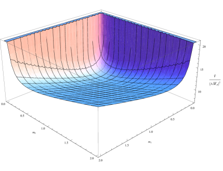
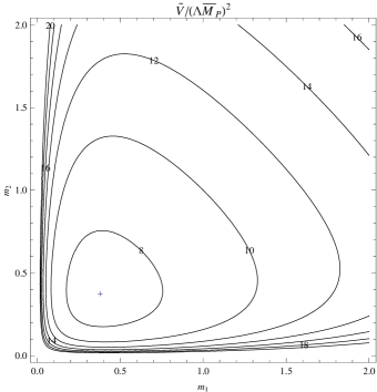
Figure 1: The shape of the potential $\widetilde{V}(\widetilde{\phi}_{i})$, defined in unit of $(\Lambda\overline{M}_{P})^{2}$, is plotted as the function, for convenience, of $m_{i}\equiv e^{\widetilde{\phi}_{i}/\overline{M}_{P}}$ ($i=1,2$) in the case of the internal manifolds being diffeomorphic to the Lie group $\mathrm{SU}(2)$. The parameters of the potential are valued as $\frac{\Lambda_{B}}{\Lambda^{2}}=5$, $a_{1}=0$, and $a_{2}=\frac{3}{4}$. Left panel: The three-dimensional plot of the given potential has an absolute minimum seen quite clearly. Right panel: The contour plot of the given potential with “+” referring the absolute minimum.

It is important that $\widetilde{V}(\widetilde{\phi}_{i})$ is emerged from the intrinsic properties of the higher dimensional space-time. Therefore, the present work may provide the natural mechanism to understand the dynamics of the extra dimensional compactification. Notice that the classical potential of the volume modulus fields can also get effective contributions from others. It is interesting to think of that the inflation can be explained in the framework in connection with the moduli stabilization attracted in much of the previous works, for example, see in radion-inflation .

Let us end this section with a few important comments on the construction of the higher dimensional gravitational interaction above. According to this description we can see that the higher dimensional gravity includes the gauge interaction of the symmetric group $G$ mediated by the gauge fields $A^{a}_{\mu}$. They are fundamental dynamic variables which are mathematically characterized to the space-time at which they define the topological non-triviality of $B^{D}$ via the Yang-Mills field strength tensor $F_{\mu\nu}$. Thus, their dynamics is to correspond with the topological dynamics of the space-time. This is clearly to be different with the usual gauge theories at which the gauge fields lay on the space-time of which is a basic manifold of a principal bundle, and the corresponding dynamics causes to the curvature of the space-time described by the dynamical metric field. Since one should not confuse this framework with that the ordinary gauge theory is coupled to the Einstein gravity and the scalars. This proposal is also completely different with the Kaluza-Klein theories. It is due to that in these theories at low energy the usual gauge fields are identified as part of the higher-dimensional metric via the Kaluza-Klein reduction. It is interesting to see that the gravity mediated by $A^{a}_{\mu}$ leads to the consistent quantum description. This means that the quantum behavior of the space-time can be understood manifestly by the quantum dynamics of the gauge fields $A^{a}_{\mu}$. A detailed study will be published elsewhere. Furthermore, this framework can also help better understanding about the gauge/gravity correspondence Maldacena98&99 ; Gubsere-Klebanov-Polyakov1998 ; Witten1998 which relates the weak coupled classical gravity to the strong coupled field theory in a flat background in one lower dimension. So far, this is only conjectured to base on studying of the string theory in which the black $p$-brane picture Horowitz-Strominger1991 in certain limit is dual to the D$p$-brane picture obtained in the weak string coupling limit of the correponding superstring theory.

IV Ground state of Bulk and perturbative gravity

IV.1 Vacuum solution of $B^{D}$

Let us look for what means actually by classical vacuum state of $B^{D}$. In the classical ground state, the matter sources are absent since the twisting of the higher dimensional bulk is obviously trivial. This means that there is a canonical splitting of $B^{D}$ into the $4$-dimensional space-time and the ($D-4$)-dimensional extra space without the gauge fields $A^{a}_{\mu}$. On other the hand, we may consider a solution describing the ground state geometry of the bulk with the topology given as

$$B^{D}=M^{4}\times G,$$ (51)

with the corresponding metric read

$$G^{0}_{MN}=\left(\begin{array}[]{cc}g_{\mu\nu}(x)&0\\ 0&e^{\langle\widetilde{\phi}_{i}\rangle/\overline{M}_{P}}\delta_{ij}\\ \end{array}\right).$$ (52)

Notice that, the ground state of $B^{D}$ must admit the internal metric associated with the stable minimum of the potential $\widetilde{V}(\widetilde{\phi}_{i})$ in which the modulus fields get VEVs denoted by $\langle\widetilde{\phi}_{i}\rangle$ (with $i=1,...,D-5$), and $\langle\widetilde{\phi}_{D-4}\rangle=0$. Indeed, this is applicable for the geometry of the ground state because $K_{i}$ (or $\hat{\partial}_{i}$) and $K^{i}$ now correspond to the basic fields of the left-invariant vector fields and one-forms on the Lie group $G$. In this case, it is interesting to result in the left-invariant metric on $G$. The above topological product implies that the vacuum geometry of the bulk is foliated by either $G$ or $M^{4}$.

By the perfect feature of the ground state geometry, we are ready to write the Einstein field equation for the external metric $g_{\mu\nu}(x)$ as follows

$$\hat{R}_{\mu\nu}-\frac{1}{2}g_{\mu\nu}(\hat{R}-\Lambda_{eff})=0.$$ (53)

Here $\hat{R}_{\mu\nu}$ and $\hat{R}$ are the Ricci and scalar curvatures, respectively, of the manifold $M^{4}$. The effective cosmological constant $\Lambda_{eff}$ is given by

$$\Lambda_{eff}=\frac{e^{-\langle\widetilde{\phi}\rangle/\overline{M}_{P}}\widetilde{V}_{\textrm{min}}}{\overline{M}^{2}_{P}},$$ (54)

where $\widetilde{V}_{\textrm{min}}$ is the value of the potential $\widetilde{V}(\widetilde{\phi}_{i})$ at its absolute minimum, and $\langle\widetilde{\phi}\rangle=\sum_{i}\langle\widetilde{\phi_{i}}\rangle/2$. The solution for Eq. (53) can be derived by the Ricci tensor satisfying in the following relation

$$\hat{R}_{\mu\nu}=\frac{\Lambda_{eff}}{2}g_{\mu\nu}.$$ (55)

This solution results in that the manifold $M^{4}$ is the $4$-dimensional Einstein space which has maximal symmetry. If $\Lambda_{eff}$ is non-zero, depending on its sign to be negative or positive, then $M^{4}$ is of the Anti de Sitter or the de Sitter space, respectively. With respect the remaining case that $\widetilde{V}_{\textrm{min}}$ vanishes where the parameters of the potential must be finely-turned to the contributions in the potential exactly canceled with each other, we have the solution of the Ricci-flat $4$-dimensional manifold. One of such ones is the $4$-dimensional Minkowski-flat space-time which has also to fulfil the stronger condition that all the components of the Riemannian tensor vanish identically. At classical level, the Minkowski space-time which is stable by the positive energy theorem WittenCMP1981 has the lowest energy. Therefore, the classical ground state for $B^{D}$ is determined by the geometry $\mathbb{R}^{1,3}\times G$ whose isometry group is the product of the $4$-dimensional Poincaré group and the Lie group $G$.

So far we have concentrated mostly to discuss the ground state of $B^{D}$ in the classical level. However, a question can be asked whether the vacuum state found above is stable or modified under the quantum effects. In the following, we would like to comment briefly about a true vacuum solution for $B^{D}$ in point of view of the quantum field theory in which the non-perturbative effects would reveal the structure of this vacuum. However, a more detailed study for such is beyond the scope of the present work but will be done in our feature work. It is important to see that the true vacuum geometry of $B^{D}$ has an extremely complicated structure due to the non-trivial topology in the space of the gauge fields. It is defined as a linear combination of topologically inequivalent energy-degenerate vacua. Each such vacuum is corresponded to a instanton number $n$ which is a geometric invariant characterizing the non-trivial topology of the bundle $B^{D}$. This quantum number is derived by integrating the second Chern character defined on the total space over a four-dimensional external manifold. The classical ground state has been looked for above to only correspond with the case of the trivial instanton number, $n=0$. On the other hand, it is inconsistent with true vacuum of $B^{D}$. Classically, the system obviously lies at the rest at a ground state with defined quantum number. Quantum-mechanically, zero-point fluctuations would play the important role which leads to the tunneling among different topological vacuum solutions, also well known as the instanton effects. Therefore, the geometry of the ground state for $B^{D}$ is precisely a superposition of these solutions presenting the quantum nature of the space-time. In this case there will not be simple to take the gauge fields $A^{a}_{\mu}$ to be zero and the globally flat metric with respect the external spaces as performed above. The instanton effects are thus expected to make some interestingly physical implications, such as in cosmology, as well as modify the classical properties of theory. Notice that, we have not been interesting in the quantum effects on the classical potential $\widetilde{V}(\widetilde{\phi}_{i})$ in the above given analysis.

IV.2 Effective dynamics of the bulk gravitation below the compactification scale

The aim of this subsection is to study the physical particle spectrum of the bulk gravity in the effective low energy theory beneath the compactification scale in which we will mainly focus the external metric field and the modulus fields. As usual, the low energy degrees of freedom of the higher dimensional gravity are obtained by the decomposition of the higher dimensional massless graviton via the KK dimensional reduction. The result includes, in the $4$-dimensional viewpoint, the massless zero modes of graviton, vectors, radion (trace of the internal metric), scalars (traceless of the internal metric), and their KK excitations Giudice1999 ; Han1999 . In the case of the internal space to be an orbifold, the zero mode of vectors will be eliminated due to the orbifold projection. For the present work, the low energy investigation of the bulk gravity may be done in a simple way. The effective degrees of freedom consist of the massive gauge bosons $A^{a}_{\mu}$ whose masses are generated by the Higgs mechanism that will be discussed in the later section and slightly perturbative fields around the classical background solution given above.

In the fact, the present observed universe is essentially flat meaning that the external spaces may be approximately considered as the $4$-dimensional Minkowski space-time. Furthermore, because of our present context which is a braneless scenario, this background is not broken by the presence of branes as their surface tension exceeds the fourth power of the fundamental Plank scale, $M^{4}_{*}$ Sundrum1999b . Since in the low energy limit we can investigate the physical progress on the bulk geometry to correspond with the above classical background.

In the weak field limit, the effective dynamics of the external metric field and the modulus fields may be studied by expanding them perturbatively around the ground state metric at the leading order as

$$g_{\mu\nu}=\eta_{\mu\nu}+M^{-1}_{\textrm{Pl}}h_{\mu\nu},\ \ \widetilde{\phi}_{i}=\langle\widetilde{\phi}_{i}\rangle+\langle V_{G}\rangle^{-\frac{1}{2}}\widetilde{h}_{i},\ \ i\neq D-4,$$ (56)

where $\eta_{\mu\nu}$ is the $4$-dimensional Minkowski background. The effective $4$-dimensional Plank scale $M_{\textrm{Pl}}$ and the vacuum volume of the internal spaces $\langle V_{G}\rangle$ are determined immediately via the fundamental parameters as follows

$$M^{2}_{\textrm{Pl}}=\frac{M^{D-2}_{*}\langle V_{G}\rangle}{\Lambda^{D-4}},\ \ \langle V_{G}\rangle=\int_{G}d^{D-4}\theta K(\theta)e^{\langle\widetilde{\phi}\rangle/\overline{M}_{P}}.$$ (57)

It is very important to note that the first equality of (57) is the usual relation to solve the hierarchy problem in the large extra-dimensional model ADDmodel with a $n$-torus of equal radii $R$ in which $\langle V_{G}\rangle/\Lambda^{D-4}\sim R^{D-4}$ and $M_{*}\sim 1\textrm{TeV}$. Notice that, the specific energy scale $\Lambda$ of the compact internal spaces in this framework should be so much larger than the inverse radii of the extra dimensions in the large extra-dimensional model. This is because all of particles are free to propagate in the whole bulk. Since such extra dimensions would not just play much the role of understanding the hierarchy problem between the weak and the Plank scales in the observed world. The $h_{\mu\nu}$ and $\widetilde{h}_{i}$ ($i\neq D-4$) express the small curvature fluctuations of the external metric and modulus fields, respectively. This means that both of them have to satisfy the condition $|h_{\mu\nu}|,|\widetilde{h}_{i}|\ll 1$. In the above given definition, these fields have been normalized so that they have the canonical kinetic term and the mass dimension. Notice that, $h_{\mu\nu}$ is the symmetric rank-$2$ tensor of ten independent components which is of the reducible representation of the $4$-dimensional Lorentz group. Thus it can be split into irreducible ones in such a way as, $2\oplus 1\oplus 0\oplus 0$. However, the fact that some degrees of freedom are consistently eliminated by constraint equations leads to the physical degrees of freedom to be less than original ones.

An effective Lagrangian determining the free evolution of $h_{\mu\nu}$ in the bulk can be obtained by inserting the first expansion of (56) into the Lagrangian (45). Then we find

$$\mathcal{L}_{h}=\frac{1}{2}\partial^{\lambda}h^{\mu\nu}\partial_{\lambda}h_{\mu\nu}-\partial^{\lambda}h^{\mu\nu}\partial_{\mu}h_{\lambda\nu}+\partial^{\mu}h\partial^{\nu}h_{\mu\nu}-\frac{1}{2}\partial^{\mu}h\partial_{\mu}h-\frac{1}{2}\left(h^{\mu\nu}\square_{G}h_{\mu\nu}+h\square_{G}h\right),$$ (58)

where $h^{\mu\nu}=\eta^{\mu\lambda}\eta^{\nu\rho}h_{\lambda\rho}$, $h=\eta^{\mu\nu}h_{\mu\nu}$, $\partial^{\mu}=\eta^{\mu\nu}\partial_{\nu}$, and $\square_{G}$ is the Laplace operator on the fixed internal spaces given as

$$\square_{G}=-\sum_{i}e^{-\langle\widetilde{\phi}_{i}\rangle/\overline{M}_{P}}{K_{i}}^{a}(\theta){K_{i}}^{b}(\theta)\hat{\partial}_{a}\hat{\partial}_{b}.$$ (59)

By the compact topology of the internal spaces, the eigenvalues of $\square_{G}$ are nonnegative and discrete. The equations of motion derived by varying $\mathcal{L}_{h}$ with respect to the perturbation $h_{\mu\nu}$ is of the form

$$\square h_{\mu\nu}-\partial_{\lambda}\partial_{\mu}h^{\lambda}_{\nu}-\partial_{\lambda}\partial_{\nu}h^{\lambda}_{\mu}+\eta_{\mu\nu}\partial_{\lambda}\partial_{\sigma}h^{\lambda\sigma}+\partial_{\mu}\partial_{\nu}h-\eta_{\mu\nu}\square h+\square_{G}\left(h_{\mu\nu}+\eta_{\mu\nu}h\right)=0.$$ (60)

We can show that both the Lagrangian (58) and Eq. (60) are invariant under the local gauge transformation

$$h_{\mu\nu}(x,\hat{\theta})\longrightarrow h_{\mu\nu}(x,\hat{\theta})-\partial_{\mu}\varepsilon_{\nu}(x)-\partial_{\nu}\varepsilon_{\mu}(x),$$ (61)

which is induced from the local external coordinate transformation. However, it is very important to see that this gauge transformation is not able to fix a gauge to eliminate some unphysical degrees of freedom. This is due to the fact that the field $h_{\mu\nu}$ is in general to depend on both the external and the internal coordinates while the gauge transformation parameters only depend on the external coordinates. It is interestingly equivalent to the interpretation that under the above gauge transformation $h_{\mu\nu}$ transforms locally on the external spaces but globally on the internal ones. The global transformation is then impossible to fix gauge hence in usual sense the transformation (61) does not generate literally the local gauge transformation. On the contrary, it would remove eight degrees of freedom to result in two physical ones for $h_{\mu\nu}$. This is of the case that the field $h_{\mu\nu}$ is independent on the internal coordinates.

The small fluctuations of the $4$-dimensional external metric can be KK expanded as

$$h_{\mu\nu}(X)=\sum_{n}h^{(n)}_{\mu\nu}(x)Y^{(n)}(\hat{\theta}),$$ (62)

where $Y^{(n)}(\hat{\theta})$ are the eigenvector of the operator $\square_{G}$ corresponding to the eigenvalue $\lambda^{2}_{n}$, with $n$ denoted to a set of quantum numbers characterizing to each eigenvector. Each KK mode $h^{(n)}_{\mu\nu}(x)$ satisfies the equations of motion in analogy with the Fierz-Pauli ones for the massive graviton but the mass term in this equation replaced by

$$\lambda^{2}_{n}\left(h^{(n)}_{\mu\nu}+\eta_{\mu\nu}h^{(n)}\right).$$ (63)

An important observation is that such mass terms clearly violate the Fierz-Pauli tuning excepting $\lambda^{2}_{0}=0$ corresponding to the massless zero mode which carries out two physical degrees of freedom. With respect to every KK excitation, we only find the constraint equations, $\partial^{\mu}h^{(n)}_{\mu\nu}+\partial_{\nu}h^{(n)}=0$, which would remove the four degrees of freedom. The constraint on the trace, $h^{(n)}=0$, is not able to be derived unless the sign of the last term in (63) is changed oppositely. Thus, each KK excited mode propagating in the effective $4$-dimensional Minkowski space-time carries exactly out six physical degrees of freedom. It is very important that this gives rise a $4$-dimensional massive graviton of five physical degrees of freedom and a real scalar ghost of instability (a scalar field with negative kinetic energy) which breaks the unitarity of theory.

The linearization of the external metric field around the classical background of $B^{D}$ yields to the unstable massive scalar excitations in the effective $4$-dimensional theory. However, a possible way to naturally overcome the problem of the scalar ghosts is that the external metric field is invariant under the action of $G$ in general up to a conformal factor as

$$g_{\mu\nu}(x,\hat{\theta}^{\prime})=e^{\sigma_{g}(x,h)}g_{\mu\nu}(x,\hat{\theta}),$$ (64)

where $\exp\{i\theta^{\prime a}T_{a}\}=\exp\{i\theta^{a}T_{a}\}h$, and $\sigma_{g}(x,h)$ is a smooth real scalar function on $B^{D}$. With the help of the local canonical section taken as

$$s:U \longrightarrow \pi^{-1}(U)$$

$$x \longmapsto s(x)=f(x,e),$$ (65)

we can particularly get an interesting and useful expression for $g_{\mu\nu}(x,\hat{\theta})$ as follows

$$g_{\mu\nu}(x,\hat{\theta})=e^{\sigma_{g}(x,\hat{\theta})}g_{\mu\nu}(x).$$ (66)

In this way, $g_{\mu\nu}(x)=g_{\mu\nu}[s(x)]$ plays the role of usual $4$-dimensional external gravity field in the effective $4$-dimensional theory. The warped scalar function $\sigma_{g}(x,\hat{\theta})$ determines the conformal diffeomorphism invariance of the external metric field under the Lie group $G$. This warped function must clearly satisfy the equation Eq. (28) but written in the case of the conformal diffeomorphism invariance. In the low energy limit, this warped factor will create a vacuum energy density, or cosmological constant contribution, which is obtained by integrating the last two terms in Eq. (58) over the vacuum volume of the internal spaces. Such density is clearly very large because of the fact that it is proportion to $\Lambda^{2}$, thus need to be exactly cancelled to other contributions, for example, the minimum energy of the moduli stabilization potential $\widetilde{V}(\widetilde{\phi}_{i})$. It is also important to notice that an interesting consequence of this invariance is that there will not occur the KK partners of the usual graviton in the effective low energy theory.This means that the important phenomenological constraints coming from the KK excitations of the usual graviton Giudice1999 ; Han1999 ; KKgraexchanges ; KKgrapro would not transparently happen in the present scenario

Next let us specialize in the physical fluctuations of the modulus fields by plugging the second expansion of (56) back into (46). Then relevant Lagrangian can be obtained as

$$\mathcal{L}_{\widetilde{h}}=\frac{1}{2}\left(\partial_{\mu}\widetilde{h}^{T}\partial^{\mu}\widetilde{h}-\widetilde{h}^{T}M_{\widetilde{h}}\widetilde{h}\right)+\mathcal{L}_{\mathrm{self-int}},$$ (67)

where $\widetilde{h}$ is a ($D-5$)-component column vector defined as, $\widetilde{h}=(\widetilde{h}_{1}...\widetilde{h}_{D-5})^{T}$, $M_{\widetilde{h}}$ is a mass mixing matrix among them, and $\partial^{\mu}=\eta^{\mu\nu}\partial_{\nu}$. The physical excitations describing the curvature perturbation of the internal spaces correspond with the eigenvectors of $M_{\widetilde{h}}$ whose masses squared, the eigenvalues of this matrix, are order of $\Lambda^{2}$. These massive scalar particles are hidden in the present world due to the compactification scale, $\sim\Lambda$, assumed to be very high compared the electroweak scale. They would be often coupled to the effective $4$-dimensional matter fields with the coupling strength, $\sim E/M_{\textrm{Pl}}$, in analogy with the usual graviton doing. Since these couplings are strongly suppressed in the energy $E$ to be so much smaller than $M_{\textrm{Pl}}$.

V $4$-dimensional Weyl fermions on bulk

In the previously higher dimensional extensions, the fundamental fermions are given as the spinorial representations of the higher dimensional Lorentz group. A problem arising from these is that beside M fermions there would have the presence of very many extra fermions, which may transform the non-triviality under the gauge group of SM, in the low energy particle spectrum. Some mechanisms have been proposed to hide these extra fermions such as the orbifold compactification Pomarol1998 ; Dienes1999 ; HCChen2000 ; Georgi2001 or using the domain wall Rubakov1983 ; Akama1982 ; Hamed2000 . In the following we expect to show in our framework that the introduction of the $4$-dimensional Weyl fermions on the bulk $B^{D}$ at fundamental level is a natural result of the intrinsical geometry of the higher dimensional space-time. The dynamics of these fermions in the bulk will then be provided in detailed investigation.

V.1 Vielbein field

Let us recall that the $4$-dimensional external tangent space at each point on $B^{D}$ spanned by $\{\hat{\partial}_{\mu}\}$ is endowed with the given metric $g_{\mu\nu}(x,\hat{\theta})$. However, one may take the vielbein field ${e_{\alpha}}^{\mu}(x,\hat{\theta})$ to change from the basis $\{\hat{\partial}_{\mu}\}$ to another basis $\{\hat{e}_{\alpha}\}$ as

$$\hat{e}_{\alpha}={e_{\alpha}}^{\mu}(x,\hat{\theta})\hat{\partial}_{\mu},$$ (68)

so that in this basis the $4$-dimensional external metric is Minkowski-flat. This therefore implies that the vierbein field must satisfy the following relation

$$\eta_{\alpha\beta}={e_{\alpha}}^{\mu}(x,\hat{\theta}){e_{\beta}}^{\nu}(x,\hat{\theta})g_{\mu\nu}(x,\hat{\theta}),$$ (69)

which defines the corresponding local $4$-dimensional Minkowski space-time at each point on $B^{D}$. The indices $\alpha$, $\beta$,… will be used to denote the local $4$-dimensional Lorentz ones. Note that the metric $\eta_{\alpha\beta}$ here would not be realized as the perturbative background metric, but is exactly the metric of the local $4$-dimensional Minkowski space-time, often called the axial metric. In the formulation of the vierbein field, the $4$-dimensional external gravity would be described by ${e_{\alpha}}^{\mu}$ instead of the metric $g_{\mu\nu}$. It is important to note that there are many local $4$-dimensional Lorentz frames that also yield of the same Eq. (69). Consequently, these will lead to the local Lorentz transformation rotating among these frames as

$${e_{\alpha}}^{\mu}(x,\hat{\theta}) \rightarrow {e^{\prime}_{\alpha}}^{\mu}(x,\hat{\theta})={\Lambda(x,\hat{\theta})^{\beta}}_{\alpha}{e_{\beta}}^{\mu}(x,\hat{\theta}),$$

$$\eta_{\alpha\beta} = {\Lambda(x,\hat{\theta})^{\gamma}}_{\alpha}{\Lambda(x,\hat{\theta})^{\sigma}}_{\beta}\eta_{\gamma\sigma},$$ (70)

where $\Lambda(x,\hat{\theta})$ is obviously an element of the Lorentz group SO$(3,1)$. The properly physical significance of this group in the case of the curved space-time is taken as the symmetry group of the local $4$-dimensional inertial frames.

From Eq. (66), the expression for the vierbein field can thus be defined as

$${e_{\alpha}}^{\mu}(x,\hat{\theta})=e^{-\frac{\sigma_{g}(x,\hat{\theta})}{2}}{e_{\alpha}}^{\mu}(x).$$ (71)

Here ${e_{\alpha}}^{\mu}(x)$ satisfies the following relation

$$\eta_{\alpha\beta}={e_{\alpha}}^{\mu}(x){e_{\beta}}^{\nu}(x)g_{\mu\nu}(x),$$ (72)

which defines the local $4$-dimensional inertial frame on an effective $4$-dimensional space-time manifold. This result also leads to, $\Lambda(x,\hat{\theta})=\Lambda(x)$, meaning that each element of the local Lorentz group SO$(3,1)$ only depends on the external coordinates.

V.2 Dynamics of $4$-dimensional Weyl fermions

Next let us proceed to discuss how the $4$-dimensional Weyl spinors occur on $B^{D}$. With the novel geometrical structure of the bulk, we may easily see that they are the simplest non-trivial irreducible representations of the local Lorentz group SO$(3,1)$ just determined above. This results in that the chiral $4$-dimensional fermions will occur naturally at the fundamental level in the present framework. Under the rotation of the local Lorentz frames, they transform as follows

$$\Psi_{L}\longrightarrow\Psi^{\prime}_{L} = e^{\frac{\mathrm{i}}{2}\xi^{m}\sigma_{m}}\Psi_{L},$$ (73)

$$\Psi_{R}\longrightarrow\Psi^{\prime}_{R} = e^{\frac{\mathrm{i}}{2}\eta^{m}\sigma_{m}}\Psi_{R},$$ (74)

where $\Psi_{L,R}$ are denoted to the left-handed and right-handed Weyl spinors written in term of the two-component spinor, respectively. They are both complex objects depending in general on the bulk coordinates. Both $\xi^{m}$ and $\eta^{m}$, with the index $m$ running from $1$ to $3$, are complex functions in only the external coordinates. These function are exactly expressed in the terms of local transformation parameters, a $4\times 4$ antisymmetric real matrix, of the group SO$(3,1)$. The matrices $\sigma_{m}$ are the usual Pauli ones. However, it is almost to work the Weyl spinors obtained from the projection of the Dirac spinor, $\Psi_{D}=(\Psi_{L}\ \ \Psi_{R})^{T}$, by the operators $P_{L,R}=(1\mp\gamma_{5})/2$. This spinor transforms under the local Lorentz group SO$(3,1)$ as

$$\Psi_{D}\longrightarrow\Psi^{\prime}_{D}=e^{\frac{i}{2}\epsilon^{\alpha\beta}\Sigma_{\alpha\beta}}\Psi_{D},$$ (75)

where $\Sigma_{\alpha\beta}=\frac{i}{4}[\gamma_{\alpha},\gamma_{\beta}]$ are the generators of the Lorentz group SO($3$,$1$) determined in terms of the usual Dirac matrices $\gamma^{\alpha}$ obeying the Clifford algebra, $\{\gamma_{\alpha},\gamma_{\beta}\}=\eta_{\alpha\beta}$. Their counterparts in the curved space-time given by $\gamma_{\mu}={e^{\alpha}}_{\mu}\gamma_{\alpha}$ satisfying the analogous one, $\{\gamma_{\mu},\gamma_{\nu}\}=g_{\mu\nu}$. The parameters $\epsilon^{\alpha\beta}$ of the above local transformation are a $4\times 4$ antisymmetric matrix with elements which are real functions in the external coordinates. In what follows we will work the Weyl spinors expressed via the Dirac spinor.

We would now like to find a suitable Lagrangian describing the propagation of the $4$-dimensional Weyl spinor fields given above in $B^{D}$. We first have to note carefully that with respect to the present case the usual kinetic term of these fields is impossible to determine the dynamics in all of directions of the bulk $B^{D}$. An obstruction is crucially due to the fact that these fields would behave the same as a spin-$1/2$ field when moving along the $4$-dimensional external directions but as a scalar field when moving in the internal directions. The scalar-like behavior is realized in sense of that the usual spin concept is lost under the viewpoint of the internal evolution in which instead of this they carry out the conventionally internal charges inherited from their non-trivial representations under the group SO$(3,1)$. This means that the physical manifestation is distinctly different to correspond with the dynamics taken in the external and internal spaces. This analysis thus give a better understanding of their dynamic properties in $B^{D}$ which will be reasonable to construct a consistent Lagrangian. Notice that it can also be straightforward for the more generic case in which fields have an arbitrary spin. A full Lagrangian thus includes two independently separating parts which determine the evolution along the external and internal directions, respectively. The evolution of such a Weyl spinor field with specifically given chirality along the $4$-dimensional external directions are characterized by the usual Lagrangian

$$\mathcal{L}^{\Psi}_{4D}=\bar{\Psi}i\gamma^{\alpha}{e_{\alpha}}^{\mu}D_{\mu}\Psi,$$ (76)

where $\Psi$ is denoted to the (right-handed) left-handed Weyl spinor field with the dimension $[\Psi]=\frac{D-1}{2}$. In particular, it may be dimensionally renormalized in the natural way as

$$\Psi_{\textrm{nor}}=\frac{\Psi}{\Lambda^{\frac{D-4}{2}}},$$ (77)

where the factor $1/\Lambda^{\frac{D-4}{2}}$ is taken from the bulk volume element. The redefinition above leads to $[\Psi_{\textrm{nor}}]=\frac{3}{2}$ which is equal to the dimension of the fermion in the $4$-dimensional space-time. It is important to note that this redefined field $\Psi_{\textrm{nor}}$ is not treated as the infraredly effective field, but it is still the fundamental field. This is because the redefinition is formally independent on a cutoff scale at which the corresponding low energy description will break down. In the following discussion we will be interesting in the renormalized fields as above in which “nor” will be dropped. On the other hand, the factor $1/\Lambda^{D-4}$ in the original matter action is completely eliminated through the redefinition of the field. The covariant derivatives $D_{\mu}$ acting $\Psi$ are given by

$$\hat{D}_{\mu}=\hat{\partial}_{\mu}+\frac{i}{2}\omega^{\alpha\beta}_{\mu}\Sigma_{\alpha\beta},$$ (78)

where $\omega^{\alpha\beta}_{\mu}$ is the torsion-free spin connection which is expressed in terms of the vierbein field as

$$\omega^{\alpha\beta}_{\mu}={e^{\alpha}}_{\nu}\left(\hat{\partial}_{\mu}e^{\beta\nu}+e^{\beta\lambda}\Gamma^{\nu}_{\mu\lambda}\right),$$ (79)

with ${e^{\alpha}}_{\nu}$ to be inverse of the vierbein field ${e_{\alpha}}^{\nu}$, and $e^{\beta\nu}=\eta^{\beta\gamma}{e_{\gamma}}^{\nu}$. It is important to notice that the $4$-dimensional Weyl spinor fields moving along the $4$-dimensional external directions with the specific chirality are massless due to their mass term vanishing. Next, let us attempt to construct an internal Lagrangian for $\Psi$. As just discussed above, in order to do this we must first find out the bilinear terms of $\Psi$ to be a Lorentz scalar which satisfying only consist of, $\bar{\Psi}^{c}\Psi$. Here $\Psi^{c}=C\Psi^{*}$ is the charge conjugate field of $\Psi$, with $*$ denoted to the complex conjugate and $C$ to be a $4\times 4$ matrix satisfying the following conditions, $C^{\dagger}C=1$ and $C^{\dagger}\gamma^{\mu}C=-\gamma^{\mu*}$. It should be noted that an another term mixing between the left-handed and right-handed Weyl spinors is not included by the property of the chirality in which they transform differently under the local gauge group. This term is thus forbidden obviously, and only generated via the coupling to the Higgs field after this field gets non-zero VEV. From the above argument, we can find out the following expectant Lagrangian

$$\mathcal{L}^{\Psi}_{G}=\frac{1}{2\Lambda}\left(-\hat{\partial}_{i}\bar{\Psi}^{c}\hat{\partial}^{i}\Psi-M^{2}_{\Psi}\bar{\Psi}^{c}\Psi\right)+\textrm{H.c.},$$ (80)

where real number $M^{2}_{\Psi}$ appearing in the above Lagrangian plays the role of mass squared characterizing to the internal motion. It thus is naturally taken to the same order as the scale $\Lambda$. We can see that this Lagrangian being analogous to that of the scalar field is quadratic in the internal derivatives $\hat{\partial_{i}}$. At first important sight, all of the terms in the Lagrangian (80) vanish identically if $\Psi$ is realized classically as the ordinary commuting field, or $c$-number. This is due to the presence of the totally antisymmetric tensor $\epsilon_{ab}$ (with $a,b=1,2$ and $\epsilon_{12}=1$) in components of the bilinear combinations of $\Psi$. This means that the internal dynamics of the $4$-dimensional Weyl spinor fields does not really make sense in the classical theory, but is of the quantum-mechanical concept in which they should be anticommuting fields. At second important one, $\Psi$ in the Lagrangian (80) is not able to play the role of the physical field under the internal point of view. This is because each term of (80) is not hermitian leading to that the corresponding Hamiltonian is unbounded from below. A combination of $\Psi$ and $\Psi^{c}$, however, defined as

$$\Psi_{M}=\Psi+\Psi^{c},$$ (81)

provides the well-defined physical field. Therefore, $\mathcal{L}^{\Psi}_{G}$ is physically rewritten as

$$\mathcal{L}^{\Psi}_{G}=\frac{1}{2\Lambda}\left(-\hat{\partial}_{i}\Psi^{T}_{M}C\hat{\partial}^{i}\Psi_{M}-M^{2}_{\Psi}\Psi^{T}_{M}C\Psi_{M}\right).$$ (82)

The field $\Psi_{M}$ is known as the Majorana spinor field (the real Dirac spinor) having the degrees of freedom to be equal to those of $\Psi$. It satisfies the reality condition, $\Psi_{M}=\Psi^{c}_{M}$, being invariant under the Lorentz transformation. The Lagrangian (82) describes the physical progress of a scalar-like neutral Grassman field in the internal spaces in which it carries out the globally SO$(3,1)$ internal symmetry in the usual sense. The structure of the KK tower for $\Psi_{M}$ is determined through the operator, $(\square_{G}-M^{2}_{\Psi})/\Lambda$. Since the lowest level has non-zero energy of the value $M^{2}_{\Psi}/\Lambda$.

In the fact, there exists a significant coupling between the modulus fields to $\Psi$ which is given by the non-trivial invariant terms in Eq. (41) coupled to $\bar{\Psi}^{c}\Psi$. At leading order, this coupling form is taken by

$$\sum^{D-5}_{i}\lambda_{\widetilde{\phi}_{i}\Psi}\widetilde{\phi}_{i}\bar{\Psi}^{c}\Psi+\textrm{H.c},$$ (83)

where $\lambda_{\widetilde{\phi}_{i}\Psi}$ are dimensionless coupling constants. Notice that, the higher-order terms in $\widetilde{\phi}_{i}$ in the coupling above are suppressed by the positive powers of $\overline{M}_{P}$ while the zero-order term leading to the mass term for $\Psi$ must obviously be zero.

It is worth stressing here one remarkable property of the internal Lagrangian given above. It may be easily verified that the Lagrangian (80) is only allowed with respect the fields which are neutral under all the local gauge charges, such as the right-handed neutrinos occurring in extensions of SM. In other words, this is not of the case of the fields of carrying out such charges, for example, the fermions of SM, due to that their Lagrangian would break the local gauge symmetry explicitly. If a $4$-dimensional Weyl spinor field $\Psi$ (for what is analyzed in the following we will still use $\Psi$ to refer the field under consideration) has the exactly conserved quantum charges, then its internal Lagrangian is precisely forbidden. Consequently, this results in that such field is by itself active (conformal) diffeomorphism invariance under the action of $G$. The values of $\Psi$ on the same internal space are thus related together. So by analogy with what has been performed for the $4$-dimensional external metric field, we can obtain an useful expression for $\Psi$ as

$$\Psi(x,\hat{\theta})=D(x,\hat{\theta})\psi(x).$$ (84)

Here $D(x,\hat{\theta})$ which is a scalar function presents the intrinsic diffeomorphism invariance of $\Psi$ under the action of $G$ and obviously satisfies Eq. (28). In low energy limit, $D(x,\hat{\theta})$ is approximately to only depend on the internal coordinates. The field $\psi(x)$ encodes the $4$-dimensional behavior of the fundamental field $\Psi$. Consequently, we assume that $\Psi$ carries additionally out the usual local gauge symmetry $G^{\prime}$, then each element of the gauge group $G^{\prime}$ does not depend on the internal coordinates. The gauge fields corresponding with the gauge group $G^{\prime}$ have thus only the $4$-dimensional external components denoted by $B_{\mu}$ which are by themselves active diffeomorphism invariance under the action of $G$ in general up to a conformal factor. This is due to that their internal Lagrangian built uniquely as

$$\sim g^{\mu\nu}\mathrm{Tr}[\hat{\partial}_{i}B_{\mu}\hat{\partial}^{i}B_{\nu}],$$ (85)

is forbidden by violating the gauge invariance.

V.3 Application to explain the smallness of the neutrino masses

Let us provide a phenomenologically significant consequence of the dynamical description for the $4$-dimensional Weyl spinor fields above. It is well established by the experimental observations that the masses of the neutrinos are so much smaller than those of the charged leptons and quarks in SM. We now desire to provide a possibility to realize the natural origin of this problem. We consider the minimal extension of SM given by including three right-handed neutrinos $\nu_{R}$ associated with three lepton families. They are all obviously singlet under the gauge group of the SM. As seen above, all of the charged leptons, the quarks and the gauge bosons of the SM are diffeomorphism invariance by themselves under the action of the Lie group $G$. Only the right-handed neutrinos and the SM Higgs doublet are to have the non-trivial dynamics in the internal spaces. The electroweak symmetry is spontaneously broken by the VEV of this scalar field whose breaking scale is possible to be much lower than the compactificated one. Hence a mass Lagrangian for the neutrinos in the flavor basis is taken in the effective low energy description as

$$\mathcal{L}^{\textrm{mass}}_{\nu}=-\sum_{n}\left(m_{n}\bar{\nu}_{L}\nu_{nR}+\frac{1}{2}M_{n}\bar{\nu}^{c}_{nR}\nu_{nR}\right)+\textrm{H.c.},$$ (86)

where $\nu_{nR}$ is the $n$th KK mode of the right-handed neutrinos, and all of the fermions have been normalized canonically. Notice that the flavor indices have been suppressed for convenience. The Dirac masses are defined by

$$m_{n}=\kappa_{n}v_{\textrm{w}},$$ (87)

where $v_{\textrm{w}}$ is the electroweak symmetry breaking scale corresponding to the VEV of the SM Higgs doublet. The dimensionless coefficient $\kappa_{n}$ contains the information about the corresponding bulk Yukawa coupling constant, the functions determining the diffeomorphism invariance of the left-handed neutrinos under $G$ and the profile wave function of the $n$th KK mode of $\nu_{R}$. Such constants are effectively matched as $4$-dimensional Yukawa coupling constants of the neutrinos. The Majorana masses occurring in a natural way in the $4$-dimensional effective theory are taken as

$$M_{n}=\frac{M^{2}_{R}}{\Lambda}+\frac{\lambda^{2}_{n}}{\Lambda}+\sum^{D-5}_{i}\lambda_{\widetilde{\phi}_{i}\nu}\langle\widetilde{\phi}_{i}\rangle.$$ (88)

The mass $M^{2}_{R}/\Lambda$ comes from the Lagrangian describing the internal dynamics for the right-handed neutrinos. The second term is mass of the $n$th KK right-handed neutrinos. The contribution by the last term is produced by the coupling between the right-handed neutrinos to the modulus fields whose form is given by (83). Therefore, the active neutrinos acquire the masses through the $5$-dimensional effective operator Weinberg1979 corresponding to the KK modes of the right-handed neutrinos integrated out as

$$m^{\mathrm{ac}}_{\nu}=m_{D}M^{-1}m^{T}_{D}.$$ (89)

Here $m_{D}$ and $M$ are ($1\times\infty$) Dirac and ($\infty\times\infty$) Majorana mass matrices, respectively, constructed from the above mass expressions. We can approximately ignore the mixing between the left-handed neutrinos and the KK excitations of the right-handed neutrinos, thus they decouple to the mass spectrum of the active neutrinos given at the lowest order

$$m_{\nu}\cong\frac{m^{2}_{0D}}{M_{0}}.$$ (90)

Eventually, the smallness of the neutrino masses at the sub-eV scale to be consistent with the neutrino oscillation data is realized via the type I seesaw mechanism which requires the scale $M_{0}$ $\sim 10^{6}$ GeV if the Dirac masses $m_{0D}$ of the neutrinos are of order of the electron mass. Therefore, we can say that the small mass appearance of the observed neutrinos is just of consequences of the higher dimensional space-time geometry.

VI Fields with internal gauge charges

In this section, we will proceed to be mainly interesting in fields on $B^{D}$ carrying out remarkable representations of the symmetry group $G$ of the internal spaces. These fields will correspond to the conventional source for the gauge fields $A^{a}_{\mu}$. Let us consider a field $\Phi(x,\hat{\theta})$ which is scalar with respect to both the local external coordinate transformation group $\textrm{GL}(4,\mathbb{R})$ and the local Lorentz group SO$(3,1)$, but carries out a $d$-dimensional representation of the Lie group $G$. This multiple is expressed in term of a column vector with $d$ scalar fields. Under the local coordinate transformations (6), the field $\Phi$ rotates as follows

$$\Phi(x,\hat{\theta})\rightarrow\Phi^{\prime}(x^{\prime},\hat{\theta}^{\prime})=U\Phi(x,\hat{\theta}),$$ (91)

where, $U=D[h(x)]=\textrm{exp}\{i\alpha^{a}(x)M_{a}\}$, is a $d\times d$ matrix corresponding to a representation of the element $h(x)\in G$ given in (6) at which $M_{a}$ are also $d\times d$ matrices associated with the representation of the generators $T_{a}\in\mathfrak{g}$. We can make an observation that the transformation (91) is nearly analogy to that in the usual gauge theory, but here it has a deep connection with the internal structure of the higher dimensional space-time. Thus, the presence of such fields in Nature would be specially useful for better intuitive understanding about the internal symmetric aspects of the higher dimensional space-time. Moreover, they would play the crucial role as the important source for the physical kinetics of $A^{a}_{\mu}$ to generate the topological twisting of the bundle $B^{D}$. A geometrical interpretation of such field is taken as a local section on the associated vector bundle with the base space $B^{D}$ rather than $M^{4}$ as in the original gauge theory.

The physical progress of the field $\Phi$ in the bulk are determined by the following Lagrangian

$$\mathcal{L}_{\Phi}=(D^{\mu}\Phi)^{{\dagger}}(D_{\mu}\Phi_{i})-(\hat{\partial}^{i}\Phi)^{{\dagger}}(\hat{\partial}_{i}\Phi)-V(\Phi),$$ (92)

where the external covariant derivatives $D_{\mu}$ are defined in a natural way by the gauge fields $A^{a}_{\mu}$ on $B^{D}$ as

$$D_{\mu}=\hat{\partial}_{\mu}+ig_{\textrm{i}}A^{a}_{\mu}M_{a}.$$ (93)

The above given Lagrangian to be invariant under (91) gives rise the gauge transformation rule as

$$A^{\prime a}_{\mu}(x^{\prime})M_{a}=\frac{\partial x^{\nu}}{\partial x^{\prime\mu}}\left[UA^{a}_{\nu}(x)M_{a}U^{-1}+\frac{1}{ig_{\textrm{i}}}U\partial_{\nu}U^{-1}\right].$$ (94)

This is to correspond with the transformation (15), but written in the form of the given representation. The infinitesimal form of (94) can be obtained with the same result as in Eq. (16).

The scalar potential $V(\Phi)$ is introduced in the following form

$$V(\Phi)=\mu^{2}\Phi^{\dagger}\Phi+\lambda(\Phi^{\dagger}\Phi)^{2}.$$ (95)

The mass squared $\mu^{2}$, as analyzed above, involves two independent masses squared, meaning that $\mu^{2}=\mu^{2}_{\mathrm{ex}}+\mu^{2}_{\mathrm{in}}$, in which $\mu_{\mathrm{ex}}$ and $\mu_{\mathrm{in}}$ are the characteristic masses for the dynamics in the external and internal spaces, respectively. The quartic-order coupling constant $\lambda$ is real and dimensionless. We have also assumed that trilinear couplings of $\Phi$ violates the gauge invariance (91) explicitly, since these are absent in the above potential. In addition, the field $\Phi$ of course couples to the modulus fields (in such a way to be similar as the field $\Psi$ discussed in the previous section coupled) and the SM Higgs doublet $H$ taken as

$$\left(\sum^{D-5}_{i}\lambda_{i}\widetilde{\phi}_{i}+\sum^{D-5}_{i,j}\lambda_{ij}\widetilde{\phi}_{i}\widetilde{\phi}_{j}\right)\Phi^{\dagger}\Phi,\ \ \lambda_{\Phi H}\Phi^{\dagger}\Phi H^{\dagger}H,$$ (96)

where the coupling constants $\lambda_{i}$ have the mass dimension whereas $\lambda_{ij}$ and $\lambda_{\Phi H}$ are dimensionless ones.

Due to the absence of the Yukawa couplings between $\Phi$ with the fermions given in the preceding section which are not allowed by the transformation (91), so the total Lagrangian possesses an accidentally exact $Z_{2}$-discrete symmetry

$$\Phi\longrightarrow-\Phi.$$ (97)

Without loss of generality, other fields can be taken to transform the trivial way (or being even) under this symmetry. Clearly, this is to come of both the symmetries of the higher dimensional space-time and the renormalizable coupling terms.

In analogy with the standard procedure to construct the kinetic term for the gauge fields in the conventional gauge theory, we need first to define the covariant field strength tensor. The easiest way to derive this tensor is through the commutator of covariant derivatives

$$\hat{F}_{\mu\nu}=\frac{1}{g_{\textrm{i}}}[D_{\mu},D_{\nu}]=-\frac{1}{\Lambda}F^{i}_{\mu\nu}\hat{\partial}_{i}+iF^{a}_{\mu\nu}M_{a}.$$ (98)

The Lagrangian for $A^{a}_{\mu}$ can then be given as

$$\mathcal{L}_{A} = \frac{1}{2}\left(\frac{M_{*}}{\Lambda}\right)^{D-4}\textbf{Tr}[\hat{F}_{\mu\nu}\hat{F}^{\mu\nu}]$$ (99)

$$= \left(\frac{M_{*}}{\Lambda}\right)^{D-4}\left(-\frac{g^{2}_{\textrm{i}}M^{2}_{*}}{4\Lambda^{2}}\sum_{i}e^{\widetilde{\phi}_{i}/\overline{M}_{P}}F^{i}_{\mu\nu}F^{i\mu\nu}-\frac{1}{4}F^{a}_{\mu\nu}F^{a\mu\nu}\right),$$

where Tr refers a symmetric inner product determined by

$$\textbf{Tr}[\hat{\partial}_{i}\hat{\partial}_{j}]=-\frac{g^{2}_{\textrm{i}}M^{2}_{*}}{2}\delta_{ij}e^{\widetilde{\phi}_{i}/\overline{M}_{P}},\ \ \textbf{Tr}[M_{a}M_{b}]=\frac{\delta_{ab}}{2},\ \ \textbf{Tr}[\hat{\partial}_{i}M_{a}]=0.$$ (100)

Comparing with (42) and the last term in (44), we can easily see that the last expression of (99) agrees with the dynamical Lagrangian for the gauge fields $A^{a}_{\mu}$.

Before proceeding to come the last section, we would like to suggest an extremely natural candidate for the dark matter (DM) coming from the scalar multiple $\Phi$ above if it is neutral under the gauge symmetry of SM. We consider the case which the $G$ gauge sector is at broken phase to be consistent with the observable fact whose scale would be higher than the electroweak scale. To maintain the multiple $\Phi$ which plays the role in the dark matter, in addition to this we should introduce a different multiple $\Phi^{\prime}$ to break spontaneously the gauge symmetry and generate masses for the gauge bosons $A^{a}_{\mu}$. Since the massive gauge bosons $A^{a}_{\mu}$ are hidden in the present observed world. For example, with $G$ to be the Lie group $\mathrm{SU}(2)$ as we already discussed previously, one can easily check a possibility that $\Phi$ and $\Phi^{\prime}$ are taken as the double and triplet of this group, respectively. This means that the vacuum would be chosen spontaneously as, $\langle\Phi\rangle=0$ (thus $\Phi$ would be realized as the inert multiple) and $\langle\Phi^{\prime}\rangle\neq 0$, which is assumed to exist. It is of the vacuum configuration described by the following surface

$$F_{\textrm{vac}}(\langle\Phi\rangle,\langle\Phi^{\prime}\rangle)=0.$$ (101)

This associates with much infinitely degenerate ground states defined classically via the vanishing of the first-order derivatives of the potential $V(\Phi,\Phi^{\prime})$. Note that due to the potential and its space of minima having the same symmetry since this minimal surface must of course have the isometric group $G$. As a consequence, the $Z_{2}$ symmetry given in (97) remains to be conserved by $\Phi$ which guarantees the stability with respect the lightest particle of the old charge under this parity. There has in general the mass splitting in $\Phi$ by coupling to $\Phi^{\prime}$. Hence the lightest component in the zero-mode of the multiple $\Phi$ is responsible to the dark matter. In this case, the SM Higgs field and the massive gauge bosons $A^{a}_{\mu}$ provides predominantly the portal which links the visible sector (the SM particles) and the dark sector whose origin is to come from the extension of the space-time structure. Notice that, these two sectors can also communicate together via higher dimension operators. Since the DM pair annihilation into the light SM particles and the DM scattering on nuclei are transmitted via both the Higgs field and $A^{a}_{\mu}$. It is important that if mass of the DM candidate is smaller than the half of the mass of Higgs boson determined by ATLAS and CMS collaborations ATLAS ; CMS , it would contribute in the invisible decay of the Higgs bosons with the current experimental data at LHC given in Belanger2013 leading to constrains on its mass and couplings. It is interesting to see that the stability of the dark matter is fully guaranteed by the intrinsically dynamical symmetry of theory rather than the symmetry imposed by the hand. To show the above given analysis more clearly, a detail study of dark matter phenomenology and constraints will be taken in Darkmatter .

VII Conclusions and Comments

This work has presented the importantly physical implications coming from a remarkably geometrical form of the $D$-dimensional space-time manifold $B^{D}$ which is assumed to occur at high energy region. It is a principal bundle constructed by attaching a smooth copy of the ($D-4$)-dimensional Lie group $G$, considered in this paper as $\mathrm{SU}(N)$ group, at each point of a $4$-dimensional pseudo-Riemannian manifold with the Lorentz metric. On the other hand, under dynamics motivated by the sources $B^{D}$ is always foliated by ($D-4$)-dimensional submanifolds deforming smoothly of $G$. These submanifolds are thought of as the internal spaces (or fibres) while the submanifolds being transversal to the fibres are realized as the external spaces which describe the usual $4$-dimensional world. The geometrical dynamics of $B^{D}$ is thus realized to associate with the high energy gravity. The corresponding fundamental degrees of freedom in the most minimal scheme consist of the gauge fields $A^{a}_{\mu}$, the $4$-dimensional external metric field $g_{\mu\nu}$ and the modulus fields $\phi_{i}$, $i=1,..,D-5$, which set dynamically the volume of the internal spaces. The presence of the gauge fields $A^{a}_{\mu}$ is to point precisely out the local directions of the external spaces which depend on the topological non-triviality of the bundle $B^{D}$. Consequently, an arbitrary particle moving along the external directions would be possible to interact with $A^{a}_{\mu}$. The corresponding gauge charges are generated dynamically by the evolution in the internal spaces. In this way, our framework is an extension of the gauge interaction in connecting closely to the structure of the space-time. All these fields are unified in the same non-trivial geometrical framework of the higher dimensional space-time. Remarkably, the potential of the moduli stabilization is constructed in a natural way that gives rise the mechanism to fix dynamically the size of the internal spaces. This is well done due to that the Lie group $G$ acts freely on $B^{D}$ and transitively on each internal space. It has been explicitly shown, for instance, the Lie group $\mathrm{SU}(2)$. By the above moduli stabilization potential, the modulus excitations have also heavy masses. The gauge fields $A^{a}_{\mu}$ get masses to become massive via the Higgs mechanism corresponding with the gauge symmetry group $G$ spontaneously broken. In this way, the mechanism to hidden the effects of the extra dimensions in the experimental seeking on accelerators is very natural. Therefore, we are completely not worry the existence of massless particles in the effective low energy theory which would lead to the unwanted violations of the equivalence principle because of contributing to Newton’s law. In summary, at the large distances, the gravity is well described by general relativity at which gravitational effects originating from extra dimensions are strongly suppressed. However, as the energy increasing highly, the usual $4$-dimensional classical gravity will get modification from such high energy effects.

We have further studied the dynamics of the $4$-dimensional Weyl spinor fields laying $B^{D}$ which are the simplest non-trivial representations of the Lorentz group $\mathrm{SO}(3,1)$. This group is determined as the local symmetry group of the local $4$-dimensional inertial frames corresponding with the Minkowski-flat form of the tangent spaces of the external spaces. The natural existence of these fields on $B^{D}$ would thus yield the very favorable light to overcome the chiral fermion problem occurring almost in the $4$-dimensional effective theory matched from the higher dimensional theory. An interesting result inherited from this description is that their physical behaviour is manifested in a distinctly different way under the dynamics in the $4$-dimensional external and internal spaces. Strictly speaking, observers will see them to behave as the spin-$1/2$ particles under the usual $4$-dimensional external point of view but as the scalar-like particles with respect to the internal point of view (i.e. their spin would be lost, and instead of this they carry out the conventional internal symmetry of the Lorentz group $\mathrm{SO}(3,1)$). Based on this analysis, the external Lagrangian for these fields has been found with the usual Dirac one but written in the curved space-time. Whereas the internal Lagrangian has the form in analogy to that of the real scalar field, but only making quantum sense without the classical equivalence. There is an important consequence related to this construction at which the internal dynamic Lagrangian is forbidden with respect to the $4$-dimensional Weyl spinor fields of carrying out the usually local gauge charges. Such fields are thus imposed by themselves the active (conformal) diffeomorphism invariance under the action of the Lie group $G$. In particular, another interesting result derived provides a possible natural interpretation for the tiny mass origin of the neutrinos observed in the present experiments via the type I see-saw mechanism.

The inclusion of the fields transforming a non-trivial way under the local symmetry group of the internal spaces is investigated in detail. They are constructed in a similar way as in the context of the usual gauge theory. A geometrical description for these fields is given as the local sections of the associated vector bundle on the $B^{D}$ rather than on the base space of $B^{D}$. The $4$-dimensional Weyl fermions discussed above are obviously neutral under this group. We also suggest a natural candidate for the dark matter coming from these novel fields to be neutral under the gauge group of the SM. An accidentally exact $Z_{2}$-discrete symmetry conserved in the broken phase of the $G$ gauge symmetry protects its stability.

Beyond those, a further issue for next work is to consider the supersymmetric extension in which the bulk space-time is included additionally the anticommuting extra dimensions NamSUSY2014 . This will be specially interesting by the fact that $B^{D}$ contains both $4$D Poincaré and gauge symmetries. Therefore, the rules of building the suppersymmetry in the previously higher dimensional space-time is clearly impossible to apply in such case.

Finally, before ending this discussion we wish to take the following useful comment. Although we have been only interesting in the internal spaces which are equivalent smoothly to the compact connected Lie group, the above given analysis will be able to be extended to some the manifolds which do not carry out the structure of the Lie group. As well known, quite many manifolds are constructed as the coset space $G/H$ that is the quotient of Lie group $G$ and its Lie subgroup $H$. If we identify physically at the points on the bulk $B^{D}$ which belong the same orbit under the action of $H$, then this result in the internal spaces which are the smooth copies of $G/H$. Note that, because the action of $H$ is free so the resulting internal spaces are also smooth manifolds unless the above identification is taken by rather the discrete subgroups than the continuous ones leading to the internal spaces with singularities, or well-known as orbifolds. These have been used in the scenarios of particle physics with extra dimensions to get the low energy realistic particle spectrum as well as the gauge symmetry or suppersymmetry breaking.

Appendix A Non-holonomic functions, Christoffel symbols and bulk scalar curvature

The frame fields on the bulk are given by, $\{E_{M}(X)\}=(\{\hat{\partial}_{\mu}\},\{\hat{\partial}_{i}\})$. The non-holonomic functions $C^{P}_{MN}$ are then determined through the Lie bracket of any two frame fields as

$$[E_{M}(X),E_{N}(X)]=C^{P}_{MN}E_{P}(X),$$ (102)

whose explicit expression is defined as follows

$$C^{\lambda}_{\mu\nu} = 0,\hskip 14.22636ptC^{i}_{\mu\nu}=-\frac{g_{\textrm{i}}}{\Lambda}F^{i}_{\mu\nu},$$ (103)

$$C^{\nu}_{\mu i}=-C^{\nu}_{i\mu} = 0,\hskip 14.22636ptC^{j}_{\mu i}=-C^{j}_{i\mu}=0,$$ (104)

$$C^{k}_{ij} = \overline{f}^{k}_{ij}.$$ (105)

With the bulk metric given generally in Eq. (34), the explicit expression for the Christoffel symbols as

$$\Gamma^{\rho}_{\mu\nu} = \frac{g^{\rho\lambda}}{2}\left(\hat{\partial}_{\mu}g_{\nu\lambda}+\hat{\partial}_{\nu}g_{\mu\lambda}-\hat{\partial}_{\lambda}g_{\mu\nu}\right),$$ (106)

$$\Gamma^{i}_{\mu\nu} = \frac{1}{2}\left(\gamma^{ij}\hat{\partial}_{j}g_{\mu\nu}-\frac{g_{\textrm{i}}}{\Lambda}F^{i}_{\mu\nu}\right),$$ (107)

$$\Gamma^{\nu}_{\mu i} = \Gamma^{\nu}_{i\mu}=\frac{g^{\nu\lambda}}{2}\left(\hat{\partial}_{i}g_{\mu\lambda}-\frac{g_{\textrm{i}}}{\Lambda}\gamma_{ij}F^{j}_{\mu\lambda}\right),$$ (108)

$$\Gamma^{j}_{\mu i} = \Gamma^{j}_{i\mu}=\frac{1}{2}\gamma^{jk}\hat{\partial}_{\mu}\gamma_{ik},$$ (109)

$$\Gamma^{\mu}_{ij} = \frac{1}{2}g^{\mu\nu}\hat{\partial}_{\nu}\gamma_{ij},$$ (110)

$$\Gamma^{k}_{ij} = \frac{1}{2}\left[\gamma^{kl}\left(\overline{f}^{m}_{li}\gamma_{mj}+\overline{f}^{m}_{lj}\gamma_{mi}\right)+\overline{f}^{k}_{ij}\right].$$ (111)

The scalar curvature of the bulk is defined by

$$R = \hat{R}+\frac{1}{4}\hat{\partial}_{i}g^{\mu\nu}\hat{\partial}^{i}g_{\mu\nu}-\frac{1}{4}\left(g^{\mu\nu}\hat{\partial}_{i}g_{\mu\nu}\right)\left(g^{\rho\lambda}\hat{\partial}^{i}g_{\rho\lambda}\right)-\frac{1}{4}\hat{\partial}_{\mu}\gamma^{ij}\hat{\partial}^{\mu}\gamma_{ij}$$ (112)

$$+\frac{1}{4}\left(\gamma^{ij}\hat{\partial}_{\mu}\gamma_{ij}\right)\left(\gamma^{kl}\hat{\partial}^{\mu}\gamma_{kl}\right)-V(\gamma_{ij})-\frac{g^{2}_{\textrm{i}}}{4\Lambda^{2}}\gamma_{ij}F^{i}_{\mu\nu}F^{j\mu\nu}+\sum^{4}_{i=1}\nabla_{M}X^{M}_{i},$$

where $\hat{R}$ is the 4-dimensional standard scalar curvature given in Eq. (49), the potential $V(\gamma_{ij})$ for the internal metric corresponding to the scalar curvature of the internal spaces is given as

$$V(\gamma_{ij})=\Lambda^{2}\left(-\frac{1}{2}f^{k}_{il}f^{l}_{kj}\gamma^{ij}+\frac{1}{4}f^{p}_{ik}f^{q}_{jl}\gamma^{ij}\gamma^{kl}\gamma_{pq}\right),$$ (113)

and

$$X^{M}_{1} = \left(-\frac{g^{\mu\nu}\gamma^{ij}\hat{\partial}_{\nu}\gamma_{ij}}{2},0\right),\ \ X^{M}_{2}=\left(0,\Lambda\frac{\gamma^{ij}g^{\mu\nu}\partial_{j}g_{\mu\nu}}{2}\right),$$

$$X^{M}_{3} = \left(\frac{g^{\mu\nu}\gamma^{ij}\hat{\partial}_{\nu}\gamma_{ij}}{2},0\right),\ \ X^{M}_{4}=\left(0,-\Lambda\frac{\gamma^{ij}g^{\mu\nu}\partial_{j}g_{\mu\nu}}{2}\right).$$

References

- (1) E. Witten, Nucl. Phys. B 186, 412 (1981).
- (2) D. Bailin and A. Love, Rep. Prog. Phys. 50, 1087 (1987).
- (3) I. Antoniadis, Phys. Lett. B 246, 377 (1990).
- (4) N. Arkani-Hamed, S. Dimopoulos, and G. Dvali, Phys. Lett. B 429, 263 (1998); I. Antoniadis, N. Arkani-Hamed, S. Dimopoulos, and G. Dvali, Phys. Lett. B 436, 257 (1998); G. Shiu and S.-H. Type, Phys. Rev. D 58, 106007 (1998).
- (5) L. Randall and R. Sundrum, Phys. Rev. Lett 83, 3370 (1999).
- (6) T. Appelquist, H.-C. Cheng, and B. A. Dobrescu, Phys. Rev. D 64, 035002 (2001); T. G. Rizzo, Phys. Rev. D 64, 095010 (2001); C. Macesanu, C.D. McMullen, and S. Nandi, Phys. Rev. D 66, 015009 (2002).
- (7) M. Bando, T. Kugo, T. Noguchi, and K. Yoshioka, Phys. Rev. Lett. 83, 3601 (1999).
- (8) T. Kugo and K. Yoshioka, Nucl. Phys. B 594, 301 (2001).
- (9) A. Dobado and A. L. Maroto, Nucl. Phys. B 592, 203 (2001).
- (10) J. Alcaraz, J. A. R. Cembranos, A. Dobado, and A. L. Maroto, Phys. Rev. D 67 075010 (2003).
- (11) R. Sundrum, Phys. Rev. D 59, 085009 (1999).
- (12) J. A. R. Cembranos, A. Dobado, and A. L. Maroto, Phys. Rev. Lett. 90, 242301 (2003); Phys. Rev. D 68, 103505 (2003).
- (13) J. A. R. Cembranos, R. L. Delgado, and A. Dobado, Phys. Rev. D 88, 075021 (2013).
- (14) Chris J. Isham, Modern Differential geometry for Physicists, World Scientific Publishing Company, Singapore (2011).
- (15) Mikio Nakahara, Geometry, Topology and Physics, Institute of Physics Publishing, London (2003).
- (16) A. Bejancu and H.R. Farran, Foliations and Geometric Structures, Springer Publishing, The Netherlands (2006).
- (17) M. Daniel and C. M. Viallet, Rev. Mod. Phys. 52, 175 (1980).
- (18) R. Jackiw, Phys. Rev. Lett. 41, 1635 (1978).
- (19) R. Jackiw, Acta Phys. Austriaca Suppl. XXII, 383 (1980); reprinted in R. Jackiw, Diverse Topics in Theoretical and Mathematical Physics (World Scientifc, Singapore, 1995).
- (20) R. Jackiw and S.-Yu. Pi, Phys. Rev. Lett. 88, 111603 (2002).
- (21) M. Gaul and C. Rovelli, Lect. Notes Phys. 541, 277 (2000).
- (22) M. Henneaux and C. Teitelboim, Foundations of Physics 16, 593 (1986).
- (23) Michael Kalb and P. Ramond, Phys. Rev. D 9, 2273 (1974).
- (24) B. Mukhopadhyaya, S. Sen, and S. SenGupta, Phys. Rev. D 65, 124021 (2002).
- (25) B. Mukhopadhyaya, S. Sen, and S. SenGupta, Phys. Rev. Lett. 89, 121101 (2002); B. Mukhopadhyaya, S. Sen, S. Sen, and S. SenGupta Phys. Rev. D 70, 066009 (2004).
- (26) T. Appelquist and A. Chodos, Phys. Rev. D 28, 772 (1983).
- (27) M. A. Rubin and B. D. Roth, Phys. Lett. B 127, 55 (1983).
- (28) E. Ponton and E. Poppitz, J. High Energy Phys. 0106, 019 (2001).
- (29) W. D. Goldberger and M. B. Wise, Phys. Rev. Lett. 83, 4922 (1999).
- (30) J.P. Derendinger, L.E. Ibáñez, and H.P. Nilles, Phys. Lett. B 155, 65 (1985).
- (31) M. Dine, R. Rohm, N. Seiberg, and E. Witten, Phys. Lett. B 156, 55 (1985).
- (32) H. P. Nilles, hep-th/0402022.
- (33) S. Weinberg, Rev. Mod. Phys. 61, 1 (1989).
- (34) R. Bousso, Gen. Rel. Grav. 40, 607 (2008).
- (35) A. Mazumdar, Phys. Lett. B 469, 55 (1999); A. M. Green and A. Mazumdar, Phys. Rev. D 65, 105022 (2002); E. W. Kolb, G. Servant, and T. M. P. Tait, JCAP 0307, 008 (2003); J. Trudeau and J. M. Cline, J. High Energy Phys. 1202, 081 (2012).
- (36) J. M. Maldacena, Adv. Theor. Math. Phys. 2, 231 (1998); Int. J. Theor. Phys. 38, 1113 (1999).
- (37) S. S. Gubser, I. R. Klebanov, and A. M. Polyakov, Phys. Lett. B 428, 105 (1998).
- (38) E. Witten, Adv. Theor. Math. Phys. 2, 253 (1998).
- (39) G. T. Horowitz and A. Strominger, Nucl. Phys. B 360, 197 (1991).
- (40) E. Witten, Commun. Math. Phys. 80, 381 (1981).
- (41) G. F. Giudice, R. Rattazzi, and J. D. Wells, Nucl. Phys. B 544 3 (1999).
- (42) T. Han, J. D. Lykken, and R. J. Zhang, Phys. Rev. D 59, 105006 (1999).
- (43) R. Sundrum, Phys. Rev. D 59, 085010 (1999).
- (44) K. Hinterbichler, Rev. Mod. Phys. 84, 671 (2012).
- (45) S. Nussinov and R. Shrock, Phys. Rev. D 59, 105002 (1999); J. L. Hewett, Phys. Rev. Lett. 82, 4765 (1999); M. L. Graesser, Phys. Rev. D 61, 074019 (2000).
- (46) N. Arkani-Hamed, S. Dimopoulos and G. R. Dvali, Phys. Rev. D 59, 086004 (1999); E. A. Mirabelli, M. Perelstein and M. E. Peskin, Phys. Rev. Lett. 82, 2236 (1999). F. Leblond, Phys. Rev. D 64, 045016 (2001).
- (47) A. Pomarol and M. Quiros, Phys. Lett. B 438, 255 (1998).
- (48) H. Cheng, B. A. Dobrescu, and C. T. Hill, Nucl. Phys. B 589, 249 (2000).
- (49) K. R. Dienes, E. Dudas, and T. Gherghetta, Nucl. Phys. B 537, 47 (1999).
- (50) H. Georgi, A. K. Grant, and G. Hailu, Phys. Rev. D 63, 064027 (2001).
- (51) V. Rubakov and M. Shaposhnikov, Phys. Rev. D 125, 136 (1983).
- (52) K. Akama, Lect. Notes Phys. 176, 267 (1982).
- (53) N. Arkani-Hamed and M. Schmaltz, Phys. Rev. D 61, 033005 (2000).
- (54) S. Weinberg, Phys. Rev. Lett. 43, 1566 (1979).
- (55) G. Aad et al. [ATLAS Collaboration], Phys. Lett. B 716, 1 (2012).
- (56) S. Chatrchyan et al. [CMS Collaboration], Phys. Lett. B 716, 30 (2012).
- (57) G. Belanger, B. Dumont, U. Ellwanger, J. F. Gunion, and S. Kraml, Phys. Lett. B 723, 340 (2013).
- (58) C. H. Nam, in preparation.
- (59) C. H. Nam, “ Gauge of extended supersymmetry in Wess-Zumino model”, in preparation.