Power spectrum tomography of dark matter annihilation with local galaxy distribution

Abstract

Cross-correlating the gamma-ray background with local galaxy catalogs potentially gives stringent constraints on dark matter annihilation. We provide updated theoretical estimates of sensitivities to the annihilation cross section from gamma-ray data with Fermi telescope and 2MASS galaxy catalogs, by elaborating the galaxy power spectrum and astrophysical backgrounds, and adopting the Markov-Chain Monte Carlo simulations. In particular, we show that taking tomographic approach by dividing the galaxy catalogs into more than one redshift slice will improve the sensitivity by a factor of a few to several. If dark matter halos contain lots of bright substructures, yielding a large annihilation boost (e.g., a factor of $\sim$100 for galaxy-size halos), then one may be able to probe the canonical annihilation cross section for thermal production mechanism up to masses of $\sim$700 GeV. Even with modest substructure boost (e.g., a factor of $\sim$10 for galaxy-size halos), on the other hand, the sensitivities could still reach a factor of three larger than the canonical cross section for dark matter masses of tens to a few hundreds of GeV.

1 Introduction

If dark matter is made of weakly interacting massive particles, as suggested by popular class of particle physics models [1], they may self-annihilate and leave observable signatures in the high-energy sky. Since the annihilation rate scales as density squared, searches for high-energy radiations such as gamma rays have been performed towards various dense regions of the sky, having yielded no definite signatures yet [2].

Since the gamma rays from dark matter annihilation precisely trace the density squared of dark matter particles, it has been proposed to study the anisotropy in the diffuse gamma-ray background to search for a characteristic signature of the dark matter annihilation [3, 4, 5, 6, 7, 8, 9, 10, 11, 12, 13, 14, 15, 16, 17]. Reference [18] analyzed the 22-month gamma-ray data from the Fermi Large Area Telescope (LAT), and detected excess in angular power spectrum over the shot noise of the photons. This excess is then interpreted to be consistent with what one expects from unresolved blazar contributions [18, 19]. No signature of dark matter annihilation has been found yet, although interesting upper limits on annihilation cross section were obtained [17, 20].

As the dark matter distribution is well traced by galaxies, Ref. [21] showed that by cross-correlating the gamma-ray map with local galaxy catalogs, one could vastly improve sensitivities on the dark matter annihilation. (See also Ref. [22].) In particular, nearby galaxy catalogs such as Two Micron All-Sky Survey (2MASS) [23] are the most ideal ones, because the most of the contributions from dark matter annihilation come from the relatively nearby Universe. Furthermore, contributions from other astrophysical sources such as star-forming galaxies (SFGs) and blazars will be suppressed, as they are more important at higher redshifts, and therefore, are less strongly correlated with the 2MASS catalogs. The expected upper limits on the annihilation cross section depend on the substructure boost just as any other extragalactic constraints, but for an optimistic boost model [24], they are sensitive to the ‘canonical’ cross section, $\langle\sigma v\rangle=(2$–$3)\times 10^{-26}$ cm³ s^-1 [1, 25], for dark matter masses smaller than a few hundreds of GeV. For a more conservative boost scenario [26], the sensitivity will be weakened by about an order of magnitude. It has also been proposed to cross correlate the gamma-ray background and weak gravitational lensing, in order to further improve sensitivities for future lensing surveys [27].

In this paper, we aim at making further theoretical developments of the cross correlation with the galaxy catalogs. In particular, we fully utilize information of redshifts of galaxies in the catalog as well as energies of photons. Specifically, we improve on the following points compared with our previous study [21].

1. Tomographic study of the cross correlation.—Galaxies in existing catalogs are in most cases assigned with either spectroscopic or photometric redshifts. Since the different redshift ranges contribute differently to the gamma-ray background depending on the sources, one could use redshift information of the catalog galaxies to further disentangle dark matter signals from the astrophysical backgrounds. Here, we divide the catalogs into several redshift bins to study sensitivities of such an approach. We show as the result that one can improve the sensitivity further by a factor of a few to several if we divide the sample into more than a few redshift bins. The same idea was mentioned for cross correlation with future lensing data in Ref. [22].

2. Improved sensitivity study.—First, we include the shot noise in the cross-power spectrum, which comes from the fact that some catalog galaxies contribute to the gamma-ray background as discrete point sources. Second, we adopt the Bayesian statistics (e.g., [28]) and Markov-Chain Monte Carlo simulations (MCMC), rather than relying on a simplistic Fisher matrix approach. This enables to use the prior information for theoretical parameters, and one can avoid any unphysical values of them such as negative values for annihilation cross section. This effect was not well treated in the previous study, and indeed, we find that the expected sensitivity is improved compared to the one from simple Fisher estimates. Third, we show that the expected sensitivity has an uncertainty range of about one order of magnitude, coming from intrinsic statistical fluctuations of data.

3. Better modeling on galaxy power spectrum and cross-correlation power spectrum.—We adopt the halo occupation distribution (HOD) within the context of ‘halo model’ [29, 30]. The galaxy power spectrum and blazar-galaxy cross-power spectrum computed this way differ substantially at small scales from the matter power spectrum. The cross power spectrum between density squared (for the dark matter annihilation) and galaxy distribution is computed in a similar way, and again, shows deviation at small scales from the cross power between density squared and density.

This paper is organized as follows. In Sec. 2, we briefly summarize models of both dark matter distribution and astrophysical sources, and give formulation and estimates of the diffuse gamma-ray background. In Sec. 3, we discuss formulation and results of the cross-correlation power spectrum, and in Sec. 4, we perform estimates of the sensitivity to the annihilation cross section, based on MCMC. Finally, we conclude the paper by giving summaries in Sec. 5. Throughout the paper, we assume the cosmological model with cold dark matter and cosmological constant ($\Lambda$CDM), and cosmological parameters adopted are $\Omega_{\rm m}=0.27$, $\Omega_{\Lambda}=0.73$, $H_{0}$ = 100 $h$ km s^-1 Mpc^-1 with $h=0.7$, $n_{s}=0.96$, and $\sigma_{8}=0.8$.

2 Diffuse gamma-ray background

This section introduces several quantities that are important for computations of the gamma-ray background intensity. We summarize it rather briefly here, but we refer the reader to our previous papers [4, 17] for a more detailed discussion.

2.1 Dark matter annihilation

The intensity of the diffuse gamma-ray background due to dark matter annihilation is proportional to the line-of-sight integral of dark matter density squared along a direction $\hat{\bm{n}}$. We write this as

$$I_{\rm dm}(\hat{\bm{n}})=\int d\chi W_{\rm dm}(z)\left[\frac{\rho_{\rm dm}(\chi\hat{\bm{n}},z)}{\langle\rho_{\rm dm}\rangle}\right]^{2}=\int d\chi W_{\rm dm}(z)[1+\delta(\chi\hat{\bm{n}},z)]^{2},$$ (2.1)

where the subscript ‘dm’ represents dark matter, $\chi$ is the comoving distance, $z$ is the redshift corresponding to $\chi$, $\rho_{\rm dm}(\chi\hat{\bm{n}})$ is the (comoving) dark matter density, and $\langle\rho_{\rm dm}\rangle=\Omega_{\rm dm}\rho_{\rm c}$ with dark matter density parameter, $\Omega_{\rm dm}=0.23$, and the critical density at the present Universe, $\rho_{\rm c}$. In the second equality, we introduced the (dark) matter overdensity $\delta=(\rho_{\rm m}-\langle\rho_{\rm m}\rangle)/\langle\rho_{\rm m}\rangle=(\rho_{\rm dm}-\langle\rho_{\rm dm}\rangle)/\langle\rho_{\rm dm}\rangle$. All the particle physics parameters such as dark matter mass $m_{\rm dm}$, annihilation cross section $\langle\sigma v\rangle$, and gamma-ray spectrum per annihilation $dN_{\gamma,{\rm ann}}/dE$ are included in the window function $W_{\rm dm}$:

$$W_{\rm dm}(z)=\frac{\langle\sigma v\rangle}{8\pi}\left(\frac{\Omega_{\rm dm}\rho_{c}}{m_{\rm dm}}\right)^{2}(1+z)^{3}\int_{E_{\rm min}}^{E_{\rm max}}dE\left.\frac{dN_{\gamma,{\rm ann}}}{dE^{\prime}}\right|_{E^{\prime}=(1+z)E}e^{-\tau(E,z)},$$ (2.2)

where $E_{\rm min}$ and $E_{\rm max}$ are the minimum and maximum energies of the photons considered, and $\tau(E,z)$ takes into account the absorption of the gamma rays due to interactions with the extragalactic background light (e.g., [31]).

We obtain the mean intensity by taking the ensemble average of Eq. (2.1):

$$\langle I_{\rm dm}\rangle=\int d\chi W_{\rm dm}(z)[1+\langle\delta^{2}(\chi)\rangle].$$ (2.3)

The variance of overdensity $\langle\delta^{2}(z)\rangle$ is computed as (e.g., [3])

$$1+\langle\delta^{2}(z)\rangle = \int dM\frac{dn(M,z)}{dM}\frac{\mathcal{J}(M,z)}{(\Omega_{\rm m}\rho_{\rm c})^{2}},$$ (2.4)

$$\mathcal{J}(M,z) \equiv [1+b_{\rm sh}(M,z)]\int dV\rho^{2}_{\rm host}(r|M),$$ (2.5)

where $dn/dM$ is the halo mass function, $\rho_{\rm host}(r|M)$ is the density profile of the host halo (i.e., smooth component), and $b_{\rm sh}(M,z)$ is the ‘boost factor’ due to presence of halo substructures. Note that the density $\rho_{\rm host}$ as well as the radial coordinate $r$ are all comoving quantities. This calculation is based on the fact that the dark matter particles are confined in halos and their subhalos, as numerical simulations show [32, 33], and hence the density squared is boosted due to enhanced clumpiness. We adopt the Navarro-Frenk-White (NFW) density profile [34] for the host halos, and with the fit, the volume integral of the density squared can be carried out analytically (see, e.g., Ref. [17]). For the halo mass function, we adopt the ellipsoidal collapse model by Ref. [35] down to a minimum mass of 10${}^{-6}M_{\odot}$. The subhalo boost factor $b_{\rm sh}(M)$ yields the largest uncertainties in this computation. In order to bracket the uncertainty, we adopt two models: one model that extrapolates the power-law dependence of the boost on subhalo masses to the smallest halo mass by Ref. [24], and the other relying on physically motivated models that well reproduce concentration parameters of the field halos but applied to the subhalos [26].

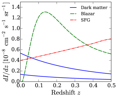
Figure 1: Contribution to the diffuse gamma-ray intensity from different redshift ranges, $dI/dz$ (left) and $dI/d\log z$ (right), for the energy band of 5–10 GeV. For dark matter, $m_{\rm dm}=100$ GeV, $\langle\sigma v\rangle=3\times 10^{-26}$ cm³ s^-1, and $b\bar{b}$ annihilation channel are assumed. The upper and lower solid curves correspond to the boost models [24, 26], respectively.

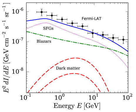
Figure 2: Spectrum of the diffuse gamma-ray background $E^{2}dI/dE$, compared with the Fermi-LAT data [36]. The models of dark matter, SFGs, and blazars are the same as in Fig. 1, and the total contribution is shown as a solid curve.

Figure 1 shows contributions to the mean intensity from different redshift ranges, $dI_{\rm dm}/dz\propto W_{\rm dm}(z)[1+\langle\delta^{2}(z)\rangle]$, for energy band of 5–10 GeV, and the two boost models [24, 26]. In this figure and also in the followings (unless stating otherwise), we assume the canonical dark matter parameters: $m_{\rm dm}=100$ GeV, $\langle\sigma v\rangle=3\times 10^{-26}$ cm³ s^-1, and annihilation channel purely into $b\bar{b}$. The dark matter contribution mainly comes from the low-redshift regime, in particular for $z\lesssim 1$. In Fig. 2, we show the spectrum of the mean intensity after integrating over all redshifts. The shape of the energy spectrum of the dark matter component is characteristic featuring bump at fraction of dark matter mass, although the amplitude is smaller than the astrophysical components or the Fermi-LAT data [36], for the dark matter parameters adopted here.

2.2 Astrophysical sources

The gamma-ray intensity due to an astrophysical source population $X$ is proportional to the line-of-sight integral of its number density $n_{X}$ as

$$I_{X}(\hat{\bm{n}})=\int d\chi W_{X}(z)\frac{n_{X}(\chi\hat{\bm{n}},z)}{\langle n_{X}(z)\rangle}=\int d\chi W_{X}(z)[1+\delta_{X}(\chi\hat{\bm{n}},z)],$$ (2.6)

where, as in Eq. (2.1), we introduced the overdensity of the source $X$ as $\delta_{X}=(n_{X}-\langle n_{X}\rangle)/\langle n_{X}\rangle$. Since $\langle\delta_{X}\rangle=0$, the mean intensity $\langle I_{X}\rangle$ is simply obtained by the integration of $W_{X}$ over $\chi$.

Often in the literature, the luminosity function is constructed from observational data to represent the (comoving) number density of the source per unit luminosity range. The luminosity is defined as the number of gamma-ray photons emitted per unit time in the source rest frame. The window function $W_{X}$ is written in terms of the luminosity function $\Phi_{X}(\mathcal{L},z)$ as

$$W_{X}(z)=\chi^{2}\int_{E_{\rm min}}^{E_{\rm max}}dE\int_{0}^{\mathcal{L}_{\rm lim}}d\mathcal{L}\Phi_{X}(\mathcal{L},z)\mathcal{F}(\mathcal{L},z),$$ (2.7)

where $\mathcal{L}$ is the differential number luminosity (number of the photons emitted per unit time per unit energy range) at energy of $(1+z)E$ and $\mathcal{F}=\mathcal{L}/(4\pi\chi^{2})$ is the differential photon flux received at energy $E$. The upper limit of the luminosity integral $\mathcal{L}_{\rm lim}$ corresponds to the sensitivity flux to point sources $F_{\rm sen}$, above which the sources are recognized as resolved and hence do not contribute to the diffuse background. These are related to each other through

$$F_{\rm sen}=\frac{1}{4\pi\chi^{2}}\int dE\mathcal{L}_{\rm lim}([1+z]E,z),$$ (2.8)

and it is straightforward to invert this relation for $\mathcal{L}_{\rm lim}$ once the spectral index is specified (see below).

As astrophysics sources, in this paper, we consider blazars and SFGs; i.e., $X=\{{\rm b},{\rm SFG}\}$, where ‘b’ stands for the blazars. These two are representative source classes that are discussed in the literature most extensively, and also their gamma-ray luminosity functions are relatively well established (in particular for the blazars). Other extragalactic sources such as radio galaxies or mis-aligned active galactic nuclei (AGNs) might also give substantial contributions, although uncertainties are much larger [37]. The main conclusion from the cross-correlation analyses reached in the subsequent sections, however, will be largely unaffected by removing these sources from our consideration. This is mainly because our approach in Sec. 4 is model independent in a sense that the amplitude of the cross-power spectrum of the astrophysical components are set as free parameters. Therefore, as also discussed in Ref. [21], unless these other sources such as mis-aligned AGNs feature an energy spectrum or clustering property very different from those of conventional astrophysical sources (that is unlikely), these components will be degenerate with either blazars or SFGs.

The blazars are further divided into two sub-classes: flat-spectrum radio quasars (FSRQs) and BL Lac objects. The gamma-ray luminosity functions of the both populations are well established from the direct measurements, and we adopt the luminosity-dependent density evolution models [38, 39]. The blazar luminosity functions are well represented with a double power law, and we impose the lower luminosity cutoff at 10⁴² erg s^-1. The spectrum of FSRQs is well approximated by a power law with an index of $2.44$, whereas that of BL Lacs is by that with an index of $2.1$ [40, 41]. For these soft and hard sources, we adopt the sensitivity flux (integrated above 100 MeV) of $F_{\rm sen}=3\times 10^{-8}$ cm^-2 s^-1 and $4\times 10^{-9}$ cm^-2 s^-1, respectively [41].

For the SFGs, we adopt the luminosity function of galaxies measured in the infrared waveband with Herschel [42], following Ref. [43]. We treat the contributions due to normal spiral galaxies and starburst galaxies separately, where the gamma-ray spectrum is approximated as $E^{-2.7}$ and $E^{-2.2}$ for the former and latter populations, respectively. The sensitivity flux for these populations are again $F_{\rm sen}=3\times 10^{-8}$ cm^-2 s^-1 and $4\times 10^{-9}$ cm^-2 s^-1, respectively. The infrared luminosity function is then converted to the gamma-ray luminosity function through the correlation between infrared luminosity and gamma-ray luminosity of the galaxies [44]:

$$\log\left(\frac{L_{\gamma}}{\mathrm{erg~{}s^{-1}}}\right)=1.17\log\left(\frac{L_{\rm IR}}{10^{10}L_{\odot}}\right)+39.28,$$ (2.9)

where $L_{\gamma}$ is the gamma-ray luminosity integrated for 0.1–100 GeV and $L_{\rm IR}$ is the infrared luminosity for 8–1000 $\mu$m.

Figure 1 also shows the astrophysical components for $dI/dz$. One can see that, unlike dark matter annihilation, these components increase with the redshifts following the trend in their luminosity functions. In particular, since blazars are bright individually (they are assumed to be brighter than 10⁴² erg s^-1 above 100 MeV), all of them within $z=0.01$ will be resolved, and there is no contribution from this component. SFGs are, on the other hand, harder to resolve individually as they are much less luminous, although they contribute to the gamma-ray background at a comparable level to the blazars. The diffuse gamma-ray background takes into account all the redshift contributions, and therefore, it is very difficult for dark matter component to excel unless its annihilation cross section is much larger than $3\times 10^{-26}$ cm³ s^-1 (Fig. 2). However, if one can single out nearby redshift regime, the dark matter component can be the dominant one, and this is realized by taking cross correlation with the local galaxy catalogs as discussed in Ref. [21] and also in the following section.

3 Cross correlation between gamma-ray background and galaxy catalogs

3.1 Galaxy catalogs

As we showed in Sec. 2.2, we are interested in extracting low-redshift information in the gamma-ray background. In the local Universe, 2MASS catalog provides nearly complete information on the galaxy distribution. In particular, 2MASS Redshift Survey (2MRS) is based on spectroscopic redshift determination of $\sim$43500 galaxies up to $z\sim 0.1$ from almost all the sky (sky coverage is $f_{\rm 2MRS}\simeq 0.91$) [23]. We approximate its redshift distribution as

$$\frac{dN_{\rm 2MRS}}{dz}\propto z\exp\left[-\left(\frac{z}{0.033}\right)^{2}\right],$$ (3.1)

where the constant of proportionality is computed such that it gives $N_{\rm 2MRS}=43500$ after integration over redshifts. We then define the 2MRS galaxy window function as $W_{\rm 2MRS}(z)=N_{\rm 2MRS}^{-1}(dN_{\rm 2MRS}/dz)(dz/d\chi)$, which gives unity after integration over the comoving distance $\chi$.

We also adopt the 2MASS Extended Source Catalog (2MXSC) as even larger sample that contains 2MRS, but with less accurate redshift determination through photometry [47, 46]. This catalog was used for the first analysis of the cross correlation of the gamma-ray background in Ref. [48]. The catalog contains $N_{\rm 2MXSC}\simeq 770000$ galaxies from the $4\pi f_{\rm 2MXSC}$-sr sky region, where $f_{\rm 2MXSC}=0.67$ [47, 48]. The redshift distribution of the catalog galaxies is

$$\frac{dN_{\rm 2MXSC}}{dz}\propto z^{1.9}\exp\left[-\left(\frac{z}{0.07}\right)^{1.75}\right],$$ (3.2)

and we define $W_{\rm 2MXSC}(z)$ similarly to that for the 2MRS catalog. We note that using extraction criteria less conservative than that of Ref. [48] will increase $f_{\rm 2MXSC}$ significantly, and hence the eventual sensitivity to dark matter.

3.2 Angular cross-power spectrum: Dark matter annihilation

The angular cross-power spectrum between the gamma-ray intensity due to dark matter annihilation $I_{\rm dm}(\hat{\bm{n}})$ and the galaxy surface density $\Sigma_{\rm g}(\hat{\bm{n}})$ (where this is normalized to $\langle\Sigma_{\rm g}\rangle=1$) is obtained as

$$C_{\rm dm,g}(\theta)\equiv\langle\delta I_{\rm dm}(\hat{\bm{n}})\delta\Sigma_{\rm g}(\hat{\bm{n}}+{\bm{\theta}})\rangle=\sum_{\ell}\frac{2\ell+1}{4\pi}C_{\ell}^{\rm dm,g}P_{\ell}(\cos\theta),$$ (3.3)

where $\delta I_{\rm dm}(\hat{\bm{n}})=I_{\rm dm}(\hat{\bm{n}})-\langle I_{\rm dm}\rangle$, $\delta\Sigma_{\rm g}(\hat{\bm{n}})=\Sigma_{\rm g}(\hat{\bm{n}})-\langle\Sigma_{\rm g}\rangle$, and $P_{\ell}(\cos\theta)$ is the Legendre polynomial. For small-angle regime, where we are mainly interested, we can approximate the sky as a flat surface, and then, the above expression simply becomes two-dimensional Fourier transform:

$$C_{\ell}^{\rm dm,g}=\int d^{2}\theta C_{\rm dm,g}(\theta)e^{-i{\bm{\ell}}\cdot{\bm{\theta}}}.$$ (3.4)

By following discussions in Appendix of Ref. [4] (see also Appendix C in the present paper), we arrive at the simple expression:

$$C_{\ell}^{\rm dm,g}=\int\frac{d\chi}{\chi^{2}}W_{\rm dm}(z)W_{\rm g}(z)P_{\delta^{2},{\rm g}}\left(\frac{\ell}{\chi},z\right),$$ (3.5)

where $P_{\delta^{2},{\rm g}}(k,z)$ is the three-dimensional cross-power spectrum between overdensity squared $\delta^{2}$ and galaxy distribution $\delta_{\rm g}=(n_{\rm g}-\langle n_{\rm g}\rangle)/\langle n_{\rm g}\rangle$.

In the framework of ‘halo model’ [49, 29, 30], where one assumes that all the matter including dark matter as well as galaxies are contained in spherical halos, the cross-power spectrum is divided into one-halo and two-halo terms:

$$P_{\delta^{2},{\rm g}}(k,z)=P^{\rm 1h}_{\delta^{2},{\rm g}}(k,z)+P^{\rm 2h}_{\delta^{2},{\rm g}}(k,z).$$ (3.6)

For the one-halo term, we cross-correlate $\delta^{2}$ and galaxies in one single halo, while for the two-halo term, we associate $\delta^{2}$ in a halo and $\delta_{\rm g}$ in another distinct halo, and take the cross correlation between these two. Therefore, once we know the distributions of both matter and galaxies within each halo, and also the intrinsic correlation between halo positions, we are able to compute the cross-correlation power spectrum. We give detailed derivation in Appendix C, and here show the formulae for both the one-halo and two-halo terms:

$$P_{\delta^{2},{\rm g}}^{\rm 1h}(k,z) = \int dM\frac{dn(M,z)}{dM}\frac{\mathcal{J}(M,z)}{(\Omega_{\rm m}\rho_{\rm c})^{2}}\frac{\langle N_{\rm g}|M\rangle}{\langle n_{\rm g}(z)\rangle}\tilde{u}_{\delta^{2}}(k|M)\tilde{u}_{\rm g}(k|M),$$ (3.7)

$$P_{\delta^{2},{\rm g}}^{\rm 2h}(k,z) = \left[\int dM\frac{dn(M,z)}{dM}\frac{\mathcal{J}(M,z)}{(\Omega_{\rm m}\rho_{\rm c})^{2}}\tilde{u}_{\delta^{2}}(k|M)b_{1}(M,z)\right]$$ (3.8)

$${}\times\left[\int dM^{\prime}\frac{dn(M^{\prime},z)}{dM^{\prime}}\frac{\langle N_{\rm g}|M^{\prime}\rangle}{\langle n_{\rm g}(z)\rangle}\tilde{u}_{\rm g}(k|M^{\prime})b_{1}(M^{\prime},z)\right]P_{\rm lin}(k,z).$$

The one-halo term has only one integration over mass function. It is multiplied by quantities related to matter and galaxy distributions. The former is represented by $\mathcal{J}\tilde{u}_{\delta^{2}}/(\Omega_{\rm m}\rho_{\rm c})^{2}$ and the latter by $\langle N_{\rm g}|M\rangle\tilde{u}_{\rm g}/\langle n_{\rm g}\rangle$, where $\langle N_{\rm g}|M\rangle$ is the number of galaxies present in a host halo with mass $M$ and $\langle n_{\rm g}\rangle$ is the average number density of the galaxies. See Appendix B.1 for more details of these quantities about the galaxies. Distribution of density squared $u_{\delta^{2}}(r)$ and that of the galaxies $u_{\rm g}(r)$ (both normalized to one after volume integration) are represented by the Fourier transform of these profiles, $\tilde{u}_{\delta^{2}}(k)$ and $\tilde{u}_{\rm g}(k)$, respectively. For the former, we adopt the same model as in Ref. [17] (see Eqs. 12–15 there) that is based on numerical simulations of subhalo distributions [24, 50], while for the latter, we assume that the (satellite) galaxies distribute following the NFW profile (see, e.g., Ref. [30] for the Fourier transform of the NFW profile). The two-halo term, on the other hand, includes two integrations over the mass function as it depends on contents in two independent halos. The one integral depends on distribution of $\delta^{2}$ and the other does on distribution of the galaxies. These two factors are connected through the intrinsic correlation between the two halos, and this halo-halo power spectrum is approximated by $P_{\rm hh}(k|M,M^{\prime})=b_{1}(M)b_{1}(M^{\prime})P_{\rm lin}(k)$, where $b_{1}(M)$ is the linear bias (e.g., [35]) and $P_{\rm lin}(k)$ is the linear matter power spectrum.

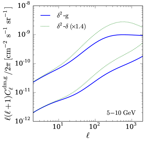
Figure 3: The angular cross-power spectrum between the gamma-ray background at 5–10 GeV due to dark matter annihilation and the 2MRS galaxies. For dark matter, $m_{\rm dm}=100$ GeV, $\langle\sigma v\rangle=3\times 10^{-26}$ cm³ s^-1, and $b\bar{b}$ annihilation channel are assumed. Upper and lower sets of curves are for the two boost models [24, 26], respectively. Solid curves are based on the density squared–galaxy power spectrum [$P_{\delta^{2},{\rm g}}(k)$], while dotted curves are on density squared–density power spectrum [$1.4P_{\delta^{2},\delta}(k)$, where 1.4 corrects for galaxy bias in the linear regime].

In Fig. 3, we show the angular cross-power spectrum between dark matter annihilation and the 2MRS galaxies for 5–10 GeV band. We here compare the resulting spectra from $P_{\delta^{2},{\rm g}}(k)$ and those from $P_{\delta^{2},\delta}(k)$ multiplied by a constant galaxy bias at linear regime (assumed to be 1.4). The $\delta^{2}$-$\delta$ power spectrum that was also adopted in Ref. [21] can be evaluated by replacing $\langle N_{\rm g}|M\rangle\tilde{u}_{\rm g}/\langle n_{\rm g}\rangle$ with $M\tilde{u}_{\delta}/(\Omega_{\rm m}\rho_{\rm c})$ in Eqs. (3.7) and (3.8). Assuming a constant, scale-independent bias of 1.4 with respect to the $\delta^{2}$-$\delta$ power spectrum will then result in an overestimate of the dark matter cross-power spectrum by up to a factor of a few in scales most relevant for possible detection. We also compare the results of the two boost models [24, 26]. The shapes for these two models are similar except for small angular scales, but the overall amplitude is larger by about an order of magnitude for the more optimistic model by Ref. [24].

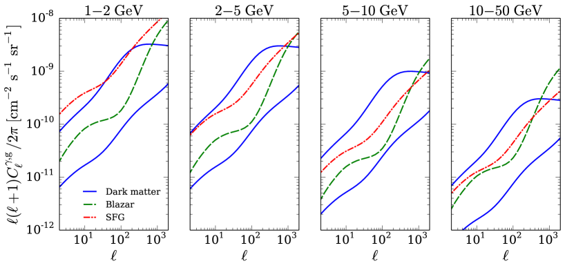
Figure 4: The angular cross-power spectrum between the 2MRS galaxies and the gamma-ray background (for four energy bands as shown at the top of each panel) due to dark matter, SFGs, and blazars. Dark matter components are evaluated for $m_{\rm dm}=100$ GeV, $\langle\sigma v\rangle=3\times 10^{-26}$ cm³ s^-1, pure $b\bar{b}$ annihilation channel, and shown for both the boost factor models [24, 26].

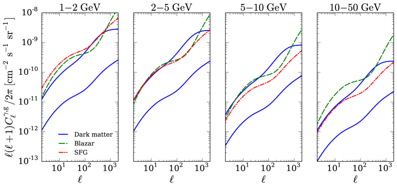
Figure 5: The same as Fig. 4 but cross-correlated with the 2MXSC galaxies.

Figures 4 and 5 show the angular power spectrum $C_{\ell}^{\rm dm,g}$, cross correlated with the 2MRS and 2MXSC galaxies, respectively, evaluated in the four energy bins: 1–2, 2–5, 5–10, and 10–50 GeV. Dark matter components (evaluated again for both the boost models [24, 26]) are compared with contributions from the astrophysical sources (see Sec. 3.3). One can see that the energy dependence as well as the shape of the power spectra are characteristic for dark matter, which will be used for distinguishing that component from the others in the following discussions.

3.3 Angular cross-power spectrum: Astrophysical sources

The total angular cross-power spectrum is the sum of all the contributions from astrophysical gamma-ray sources as well as dark matter annihilation. Here, as in Sec. 2.2, we consider the SFGs and blazars as such representative astrophysical sources, $X=\{{\rm SFG,b}\}$. Since most of them are regarded as point-like gamma-ray sources for Fermi-LAT, and they may overlap with catalog galaxies in 2MRS or 2MXSC, the cross-power spectrum will also include the stochastic shot noise that comes from the discrete nature of some sources. Therefore, the total cross-power spectrum is written as

$$C_{\ell}^{\gamma,{\rm g}}=C_{\ell}^{\rm dm,g}+\sum_{X}\left(C_{\ell}^{X,{\rm g}}+C_{\rm P}^{X,{\rm g}}\right),$$ (3.9)

where $C_{\rm P}^{X,{\rm g}}$ represents the shot (or Poisson) noise of the source $X$. The shot-noise term, as we derive in Appendix A, depends on the number density of the relevant sources, and results in being independent of scales or multipoles $\ell$. Therefore, it is relatively straightforward to subtract this scale-independent component from the total power spectrum, but such a procedure induces errors.

The angular cross-power spectrum between the gamma-ray background due to a source class $X$ and catalog galaxies g, $C_{\ell}^{X,{\rm g}}$, is evaluated similarly as $C_{\ell}^{\rm dm,g}$ in the previous subsection:

$$C_{\ell}^{X,{\rm g}}=\int\frac{d\chi}{\chi^{2}}W_{X}(z)W_{\rm g}(z)P_{X,{\rm g}}\left(\frac{\ell}{\chi},z\right),$$ (3.10)

where $P_{X,{\rm g}}(k,z)$ is the cross-power spectrum between $X$ and the galaxies (excluding the shot-noise component). We once again base our approach on the halo model, and give details in Appendices B.1 and B.2, for the SFGs and blazars, respectively. Here, we simply give qualitative arguments of the model and show results of the cross-power spectra.

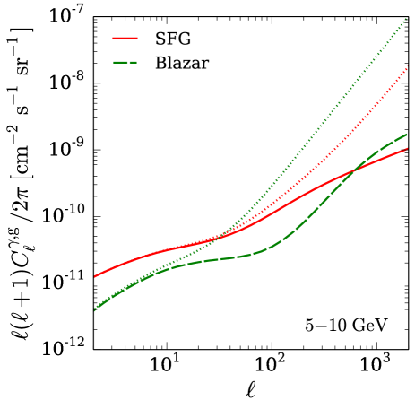
Figure 6: The angular cross-power spectrum between the gamma-ray background at 5–10 GeV due to SFGs (solid) or blazars (dashed) and the 2MRS galaxies. Dotted curves include the shot-noise terms, $C_{\rm P}^{\rm SFG,g}$ and $C_{\rm P}^{\rm b,g}$.

The galaxy power spectrum $P_{\rm g}(k,z)$ is the relevant quantity for SFGs. Within the framework of the halo model, this can be evaluated once we specify a number of galaxies in a halo with mass $M$, $\langle N_{\rm g}|M\rangle$, and how they are distributed in it. The angular cross-power spectrum for this component is shown in Fig. 6 for the 5–10 GeV energy band, and is compared with the shot noise associated with it. The shot noise starts dominating at small scales, $\ell\gtrsim 200$, and thus one cannot ignore such a term.

Clustering properties of the gamma-ray blazars are much less understood, mainly because of paucity of detected sources. We here assume that the gamma-ray blazars are well correlated with AGNs identified with X rays. In fact, the blazar luminosity functions adopted here [38, 39] are constructed relying on the same argument. By studying the distribution of X-ray AGNs, Refs. [51, 52] found that they appear to selectively locate in dark matter halos with mass around $\sim$10${}^{13.1}\,h^{-1}M_{\odot}$. Following this, we assume that the gamma-ray blazars also live in these halos (at the center), whose bias parameter is then obtained as the one for their host halos, and also that there is no more than one blazar in each halo. We show the angular power spectrum for blazars calculated this way in Fig. 6, cross-correlated with the 2MRS galaxies, as well as the shot-noise component. Since fewer and brighter blazars contribute to the gamma-ray background compared with SFGs, they yield larger shot-noise term, which becomes dominant already at $\ell\sim 30$.

Figures 4 and 5 summarize the energy dependence of both the blazar and SFG components, cross-correlated with the 2MRS and 2MXSC galaxies, respectively.

4 Sensitivity to annihilation cross section

4.1 Covariance matrix and errors of cross correlation

We consider gamma-ray maps $\gamma_{i},\gamma_{j},\cdots$ and galaxy catalogs ${\rm g}_{a},{\rm g}_{b},\cdots$, where one can think that $i,j,\cdots$ represent energy bins, and $a,b,\cdots$ do redshift bins. If we consider one catalog (such as 2MRS or 2MXSC) as a whole, then there is only one redshift bin to be considered. Covariance between $C_{\ell}^{\gamma_{i},{\rm g}_{a}}$ and $C_{\ell}^{\gamma_{j},{\rm g}_{b}}$ is given by (e.g., [53, 15])

$$\mbox{Cov}\left(C_{\ell}^{{\gamma_{i}},{\rm g}_{a}},C_{\ell}^{\gamma_{j},{\rm g}_{b}}\right)=\frac{1}{(2\ell+1)f_{\rm sky}}\left[C_{\ell}^{\gamma_{i},{\rm g}_{b}}C_{\ell}^{\gamma_{j},{\rm g}_{a}}+\left(C_{\ell}^{\gamma_{i},\gamma_{j}}+\delta_{ij}\frac{C_{\rm N}^{\gamma_{i}}}{W_{\ell}^{i2}}\right)\left(C_{\ell}^{{\rm g}_{a},{\rm g}_{b}}+\delta_{ab}C_{\rm N}^{{\rm g}_{a}}\right)\right],$$ (4.1)

where $f_{\rm sky}$ is the fraction of sky covered by the survey, $\delta_{ij}$ and $\delta_{ab}$ are the Kronecker delta, $C_{\rm N}^{\gamma_{i}}$ and $C_{\rm N}^{{\rm g}_{a}}$ are the shot noise of the photons in the energy bin $i$ and that of the galaxies in the redshift bin $a$, respectively, and $W_{\ell}^{i}$ is the Fourier transform of the point-spread function in the energy band $i$.

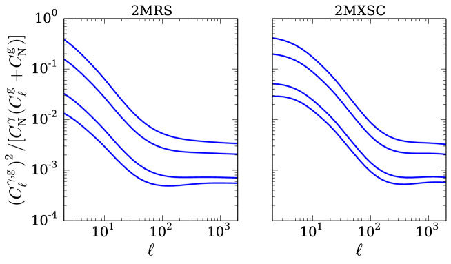
Figure 7: The ratio between cross-power spectrum squared and product of gamma-ray and galaxy auto-power spectra, $(C_{\ell}^{\gamma,{\rm g}})^{2}/[C_{\rm N}^{\gamma}(C_{\ell}^{\rm g}+C_{\rm N}^{\rm g})]$, for the 2MRS (left) and 2MXSC (right) galaxies. Four curves in each panel correspond to the energy bands, 1–2, 2–5, 5–10, and 10–50 GeV (from top to bottom). A plateau for $\ell\gtrsim 100$ is due to shot noise in the cross power.

If two redshift bins do not overlap, as we postulate in this paper, then there is no cross correlation in the galaxy power spectrum; the galaxies in different redshift ranges are uncorrelated, i.e., $C_{\ell}^{{\rm g}_{a},{\rm g}_{b}}=\delta_{ab}C_{\ell}^{{\rm g}_{a}}$ (see also discussions at the end of this subsection). One cannot argue in a similar way for $C_{\ell}^{\gamma_{i},\gamma_{j}}$, because a bright source in one energy bin $i$ tends to be also bright in another energy bin $j$. In practice, however, the photon shot noise $C_{\rm N}^{\gamma}$ is much larger than the angular auto-power spectrum $C_{\ell}^{\gamma}$ from the anisotropy measurement with Fermi [18], and therefore one can treat the second term in the square bracket of Eq. (4.1) as a diagonal matrix proportional to $\delta_{ij}\delta_{ab}$. We can further show that the first term is negligible compared with the second, by explicitly computing $(C_{\ell}^{\gamma,{\rm g}})^{2}$ and comparing it with $C_{\rm N}^{\gamma}(C_{\ell}^{\rm g}+C_{\rm N}^{\rm g})$. Figure 7 shows $(C_{\ell}^{\gamma,{\rm g}})^{2}/[C_{\rm N}^{\gamma}(C_{\ell}^{\rm g}+C_{\rm N}^{\rm g})]$ for both the 2MRS and 2MXSC galaxies and various energy bins, which is indeed found to be smaller than one in any of these cases. If we divide these catalogs into redshift bins, then the galaxy shot noise $C_{\rm N}^{{\rm g}}$ increases, yielding even smaller values for this ratio. Therefore, we can safely approximate Eq. (4.1) as a diagonal matrix:

$$\mbox{Cov}\left(C_{\ell}^{\gamma_{i},{\rm g}_{a}},C_{\ell}^{\gamma_{j},{\rm g}_{b}}\right)\approx\delta_{ij}\delta_{ab}\left(\delta C_{\ell}^{\gamma_{i},{\rm g}_{a}}\right)^{2},$$ (4.2)

where the diagonal components are given as

$$\left(\delta C_{\ell}^{\gamma_{i},{\rm g}_{a}}\right)^{2}=\frac{1}{(2\ell+1)f_{\rm sky}}\left[\left(C_{\ell}^{\gamma_{i},{\rm g}_{a}}\right)^{2}+\left(C_{\ell}^{\gamma_{i}}+\frac{C_{\rm N}^{\gamma_{i}}}{W_{\ell}^{i2}}\right)\left(C_{\ell}^{{\rm g}_{a}}+C_{\rm N}^{{\rm g}_{a}}\right)\right].$$ (4.3)

For the sensitivity study below, we adopt $f_{\rm sky}=0.7$, $C_{\rm N}^{\gamma_{i}}=I_{\rm obs}^{i}/\mathcal{E}$, $C_{\rm N}^{{\rm g}_{a}}=4\pi f_{\rm g}/N_{{\rm g}_{a}}$, where $I_{\rm obs}^{i}$ is the observed mean intensity in the energy band $i$ reported in Ref. [36], $\mathcal{E}=1.5\times 10^{11}$ cm² s is five-year exposure of Fermi-LAT, $N_{{\rm g}_{a}}$ is the number of the catalog galaxies contained in redshift bin $a$ from $4\pi f_{\rm g}$ sr of the sky; $N_{\rm g}=43500$ (770000) and $f_{\rm g}=0.91$ (0.67) for 2MRS (2MXSC) without redshift binning. The angular auto-power spectrum of the gamma-ray background $C_{\ell}^{\gamma_{i}}$ is found to be dominated by shot-noise due to the blazars [18, 19], and we adopt these measured values. For the angular response represented by $W_{\ell}^{i}$, we use the results reported in Ref. [18]. We also note that $C_{\ell}^{\gamma_{i},{\rm g}_{a}}$ in the right-hand side of Eq. (4.3) includes the shot-noise component.

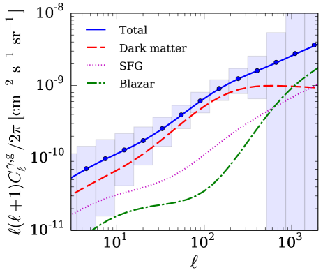
Figure 8: The angular cross-power spectrum between the gamma-ray background in the 5–10 GeV band and the 2MRS galaxies, and expected $1\sigma$ errors (boxes). Dark matter component is evaluated for $m_{\rm dm}=100$ GeV, $\langle\sigma v\rangle=3\times 10^{-26}$ cm³ s^-1, pure $b\bar{b}$ annihilation channel, and for the boost model by Ref. [24].

As an example of error estimates, Fig. 8 shows the expected errors for the total cross-power spectrum (after subtracting the shot-noise component) between the gamma-ray background in the 5–10 GeV energy band and the 2MRS galaxies, for the boost model by Ref. [24]. The expected errors are very small compared with the signal, and therefore, if this were the case, the dark matter component would be clearly detected. We also note that the prospect is even better than the one from our previous study. One can see this by comparing Fig. 8 with Fig. 2 of Ref. [21]. This comes from difference of the models adopted; here we adopt the cross-power spectrum based on the HOD of galaxies within halo model, whereas in Ref. [21], we simply assumed that galaxies trace matter with a constant bias. As the result of this difference, our present model yields larger cross power, and hence smaller relative errors.

Table 1: Galaxy catalogs for cross correlation. The boundaries of the redshift binning and the number of galaxies per bin are shown in the second and the third columns, respectively.

Catalog	Redshift boundaries	$N_{\rm g}$ per bin
2MRS	(0.003, 0.1)	43500
2MRS-N2	(0.003, 0.027, 0.1)	21750
2MRS-N3	(0.003, 0.021, 0.035, 0.1)	14500
2MXSC	(0.003, 0.3)	770000
2MXSC-N2	(0.003, 0.083, 0.3)	385000
2MXSC-N3	(0.003, 0.066, 0.10, 0.3)	257000
2MXSC-N4	(0.003, 0.058, 0.083, 0.11, 0.3)	193000
2MXSC-N5	(0.003, 0.052, 0.073, 0.093, 0.12, 0.3)	154000
2MXSC-N10	(0.003, 0.039, 0.052, 0.063, 0.073,	77000
	0.083, 0.093, 0.10, 0.12, 0.14, 0.3)

The redshift binning is simply done such that each bin contains the same number of galaxies. Table 1 summarizes the catalogs and the redshift binning. For example, 2MXSC-N5 is based on the 2MXSC catalog, but we divide it into five redshift bins, each of which contains 154000 galaxies. When we use a finer redshift binning, more information is made available. However, one starts to see correlation between two neighboring redshift bins, if their widths are too small. This may be estimated by comparing the width with the galaxy correlation length—the length at which the two-point correlation function $\xi_{\rm g}$ becomes one. We find this length to be $\sim$10 Mpc, by computing $\xi_{\rm g}$ from the Fourier transform of the galaxy power spectrum $P_{\rm g}(k)$ in the local Universe ($z=0$). The finest redshift slices are obtained for 2MXSC-N10, where $(\Delta z)_{\rm min}=0.01$ and this corresponds to the comoving distance of $\sim$40 Mpc. This is reasonably larger than the galaxy correlation length, and in fact the galaxy two-point correlation function at the separation of 40 Mpc is only 0.09.

Another important quantity to compare the width of redshift bins with is the accuracy of the photometric-redshift determination, in the case of 2MXSC. The latest analysis of the 2MASS photometric redshift catalog shows that the redshift accuracy is about 12% [54]. For typical 2MXSC galaxies around $z\sim 0.1$, this corresponds to the accuracy of $\sigma_{z}\sim 0.01$, which is comparable to the smallest bin width for 2MXSC-N10. Therefore, the redshift slicing using more than several bins might induce correlation between neighboring redshift bins. As we shall show in Sec. 4, however, the sensitivity to the annihilation cross section saturates when using a few redshift bins already, and therefore, this uncertainty results in no major impact on our conclusions.

4.2 Bayesian statistics and prior distributions

We adopt the Bayesian statistics (e.g., [28]) in order to obtain the sensitivity to the annihilation cross section. Given data $\{\bm{d}\}$, the posterior probability distribution function of parameters $\{\bm{\vartheta}\}$ is constructed as

$$P({\bm{\vartheta}}|{\bm{d}})\propto P({\bm{\vartheta}})P({\bm{d}}|{\bm{\vartheta}}),$$ (4.4)

where $P(\bm{\vartheta})$ is the prior of the parameters and $P({\bm{d}}|{\bm{\vartheta}})$ is the likelihood function—the probability of obtaining the data $\{\bm{d}\}$ given the parameters $\{\bm{\vartheta}\}$. In general, functional form of the posterior is undefined, and in such a case, a powerful and efficient approach to estimate it is to perform the MCMC.

The data $\{\bm{d}\}$ are obtained only through relevant analysis of the gamma-ray maps cross-correlated with galaxy catalogs. It is, however, beyond the scope of this paper, as our aim is to evaluate potential sensitivities of the cross-correlation analysis to dark matter parameters, especially the annihilation cross section. Therefore, for the current purpose, it suffices to construct ‘data’ from the model itself. The model is defined with fixed values of dark matter mass $m_{\rm dm}$ and shapes of the cross-power spectra. As parameters {$\bm{\vartheta}$} that vary, we consider the following four: the annihilation cross section $\langle\sigma v\rangle$, the amplitudes of the cross-power spectra for blazars $\vartheta_{\rm b}$ and for SFGs $\vartheta_{\rm SFG}$, and amplitude of the shot-noise component $\vartheta_{\rm P}$. The data of the cross-power spectra are assumed to be the same as a model, with no dark matter component ($\langle\sigma v\rangle=0$), but assuming that both the blazar and SFG contributions are described by the reference models given in Sec. 3.3, and we normalize the parameters to $\vartheta_{\rm b}=1$, $\vartheta_{\rm SFG}=1$, and $\vartheta_{\rm P}=1$ in this reference case:

$${\bm{d}}\equiv\left(C_{\ell}^{\gamma_{i},{\rm g}_{a}}\right)_{\rm data}=\sum_{X=\{{\rm b,SFG}\}}\left[\left(C_{\ell}^{X_{i},{\rm g}_{a}}\right)_{\rm ref}+\left(C_{\rm P}^{X_{i},{\rm g}_{a}}\right)_{\rm ref}\right],$$ (4.5)

where the subscript ‘ref’ stands for the reference theoretical models.

The likelihood function is then obtained as the product of (assumed) Gaussian distribution of the cross-power spectrum as follows:

$$P(\bm{d}|\bm{\vartheta}) \propto \frac{1}{(\det\mbox{Cov})^{1/2}}\exp\left\{-\frac{1}{2}\left[{\bm{d}}-{\bm{C}}(\bm{\vartheta})\right]^{T}\mbox{Cov}\left[{\bm{C}}(\bm{\vartheta}),{\bm{C}}(\bm{\vartheta})\right]^{-1}\left[{\bm{d}}-{\bm{C}}(\bm{\vartheta})\right]\right\}$$

$$\approx \prod_{i}\prod_{a}\prod_{\ell}\frac{1}{\delta C_{\ell}^{\gamma_{i},{\rm g}_{a}}(\bm{\vartheta})}\exp\left\{-\frac{1}{2}\left[\frac{\left(C_{\ell}^{\gamma_{i},{\rm g}_{a}}\right)_{\rm data}-C_{\ell}^{\gamma_{i},{\rm g}_{a}}\left(\bm{\vartheta}\right)}{\delta C_{\ell}^{\gamma_{i},{\rm g}_{a}}(\bm{\vartheta})}\right]^{2}\right\},$$

$$\bm{C}(\bm{\vartheta}) \equiv C_{\ell}^{\gamma_{i},{\rm g}_{a}}(\bm{\vartheta})=\frac{\langle\sigma v\rangle}{\langle\sigma v\rangle_{\rm ref}}\left(C_{\ell}^{{\rm dm}_{i},{\rm g}_{a}}\right)_{\rm ref}+\vartheta_{\rm b}\left(C_{\ell}^{{\rm b}_{i},{\rm g}_{a}}\right)_{\rm ref}+\vartheta_{\rm SFG}\left(C_{\ell}^{{\rm SFG}_{i},{\rm g}_{a}}\right)_{\rm ref}$$ (4.7)

$${}+\vartheta_{\rm P}\left[\left(C_{\rm P}^{{\rm b}_{i},{\rm g}_{a}}\right)_{\rm ref}+\left(C_{\rm P}^{{\rm SFG}_{i},{\rm g}_{a}}\right)_{\rm ref}\right],$$

where $\langle\sigma v\rangle_{\rm ref}=3\times 10^{26}$ cm³ s^-1. In the second equality of Eq. (LABEL:eq:likelihood), we approximated the covariance matrix as diagonal [Eq. (4.2)], and in the denominator of the last expression of the same equation, we use Eq. (4.3) but with $C_{\ell}^{\gamma_{i},{\rm g}_{a}}(\bm{\vartheta})$ in its right-hand side.

For the prior $P(\bm{\vartheta})$, we assume flat distributions in logarithmic space for the following ranges: $-30<\log(\langle\sigma v\rangle/\mathrm{cm^{3}~{}s^{-1}})<-20$, $-5<\log\vartheta_{\rm b}<2$, $-5<\log\vartheta_{\rm SFG}<2$, and $-2<\log\vartheta_{\rm P}<2$. These cover sufficiently large volume in the parameter space. This is a conservative approach, as we do not use information from any other measurements such as amplitudes for luminosity functions of SFGs and blazars.

4.3 Markov-Chain Monte Carlo simulations and sensitivity estimates

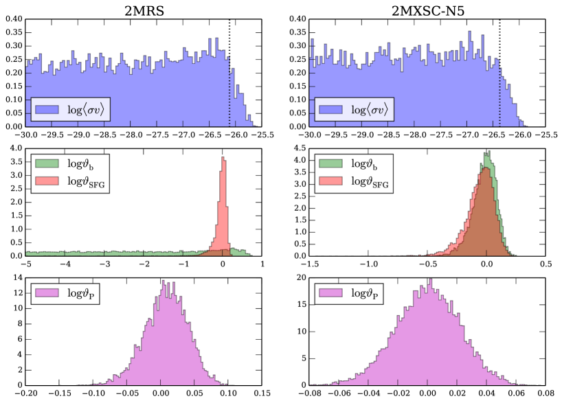
Figure 9: Posterior distributions of parameters ($\langle\sigma v\rangle$, $\vartheta_{\rm b}$, $\vartheta_{\rm SFG}$, and $\vartheta_{\rm P}$) for 2MRS (left) and 2MXSC-N5 (right). The dark matter mass is 100 GeV and the boost model is by Ref. [24]. The dotted vertical lines in the top panels indicate the 95% credible upper limit.

We obtain the posterior distributions of the parameters $\{\bm{\vartheta}\}$ by running MCMC. Figure 9 shows them for 2MRS (left) and 2MXSC-N5 (right), in the case of the 100-GeV dark matter annihilating purely into $b\bar{b}$ and the optimistic boost model [24]. First, the shot-noise component is well determined from its scale-independent feature, in particular important at high multipoles. The posterior distribution of $\vartheta_{\rm P}$ has width of only a few to several percent (bottom panels). The SFGs can also be determined relatively well, but the blazar component is unconstrained by using the 2MRS catalog (middle left panel). This is due to limited redshift information available for the 2MRS catalog, and therefore, can be improved by using more than one redshift bin as shown, e.g., in the case of 2MXSC-N5 (middle right panel). Since the ‘data’ do not contain any dark matter component, we have the posterior distribution of $\langle\sigma v\rangle$ featuring tail at low values. Too large values, however, are not allowed as they become seriously in conflict with the data; hence the distribution features upper cutoff (top panels). (The same argument applies to $\vartheta_{\rm b}$ in the case of 2MRS.) By integrating this posterior distribution up to some value such that the integral yields 95% of the total area, one can set the 95% credible upper limit. The upper limit computed this way is shown as dotted vertical lines in the top panels.

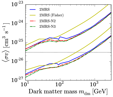
Figure 10: 95% credible sensitivities to the annihilation cross section as a function of dark matter mass, obtained from cross correlation between the five-year Fermi data for the gamma-ray background and the galaxy catalogs (2MRS, 2MRS-N2, and 2MRS-N3). Sensitivities based on Fisher matrix as in Ref. [21] are also shown for comparison. Lower and upper sets of the curves correspond to the results for the different boost models [24, 26], respectively. The dotted horizontal line represents the canonical annihilation cross section for thermal production in the early Universe.

We performed the MCMC described above for all the galaxy catalogs summarized in Table 1 and for various dark matter masses. In Fig. 10, we show 95% credible sensitivities to the annihilation cross section as a function of dark matter mass, for the different boost models [24, 26]. We also show the upper limits for 2MRS using the Fisher matrix, calculated as in Ref. [21] by varying all the four parameters. First, we see that the five-year sensitivity for the 2MRS catalog obtained with MCMC is better than the estimate obtained with the Fisher matrix, especially at high-mass regime. In particular, for the optimistic boost case [24], one would be able to exclude the canonical annihilation cross section for dark matter less massive than $\sim$700 GeV. This difference comes from the fact that the method relying on MCMC is capable of adopting the prior distribution, hence avoiding unphysical parameter ranges such as negative values for the amplitudes, etc. Second, by subdividing the 2MRS catalog into a few redshift bins, one can further improve the sensitivity by up to a factor of two. The improvement appears to saturate already for the 2MRS-N2 model. Third, even for the conservative boost scenario [26], the sensitivity to the cross section is encouragingly close to its canonical value for thermal production of dark matter particles. It features a plateau from tens to a few hundreds of GeV around $\sim$10^-25 cm³ s^-1.

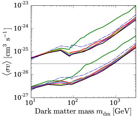
Figure 11: The same as Fig. 10 but for 2MXSC (top solid) and for 2MXSC-N2 to 2MXSC-N10 (bottom solid curves). The results for 2MRS are shown for comparison as dashed curves.

Figure 11 shows the same sensitivity to the annihilation cross section as Fig. 10, but for the larger galaxy catalog 2MXSC. Even though it is larger, more astrophysical contamination from the high-redshift regime will weaken the sensitivity compared to the case with 2MRS. The tomographic approach, however, proves to be much more efficient in this case. If we divide the 2MXSC catalog into two redshift bins (2MXSC-N2), the expected sensitivity improves already by a factor of several for the mass range larger than 100 GeV. There are no further major improvements even if we sub-divide the catalog into finer redshift slices. We show all the results of the sensitivity from 2MXSC-N2 to 2MXSC-N10. Compared with the 2MRS limits, one could improve up to a factor of three.

Until this point, we assumed that the data are perfectly the same as our reference model without dark matter [Eq. (4.5)], and correspondingly obtained the sensitivities to the annihilation cross section. In reality, however, data fluctuate statistically, and as the result, the associated sensitivity estimates also do. In order to estimate significance of such fluctuations, we generated data from Monte Carlo simulation. More specifically, for one Monte Carlo realization, we simulate data from the Gaussian distribution with the mean of Eq. (4.5) and variance of Eq. (4.3) (again assuming no dark matter component). The 95% credible sensitivities to the annihilation cross section for this data set were then obtained with the same MCMC procedure as above. We repeated such a procedure a number of times to obtain the distribution of the expected sensitivities.

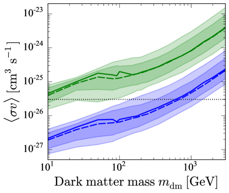
Figure 12: The 68% and 95% containment intervals of the 95% credible sensitivity to the annihilation cross section, from cross correlation with 2MRS and for both the boost models [24, 26]. The dashed curves are the median of the distribution, while the solid curves are the same as shown in Fig. 10.

The results in the case of cross correlation with 2MRS are shown in Fig. 12 as thick and thin bands, with which we show 68% and 95% containment intervals of the 95% credible sensitivities. The median of the distribution is shown as the dashed curves, while the solid curves are the same as the ones shown in Fig. 10. We find that fluctuation of cross-correlation data yields difference of the upper limits on the annihilation cross section by almost one order of magnitude.

5 Conclusions

As was pointed out in Ref. [21], taking cross correlation between the gamma-ray background (due to Fermi-LAT) and the local galaxy distribution such as 2MASS catalogs provides very efficient way of constraining dark matter annihilation cross section. This is because the dark matter annihilation contributes more to the gamma-ray background from the local Universe at lower redshifts.

In this paper, we aimed at making further theoretical progress. Most importantly, since galaxies in major catalogs are assigned with either spectroscopic or photometric redshifts, one could further use this information to disentangle dark matter from other astrophysical sources. Taking such a tomographic approach, we divided the 2MASS catalogs into more than one (up to ten) redshift bins. We found that we could already improve the sensitivities to the annihilation cross section by a factor of a few to several, if we divided the catalogs into two or three redshift slices. Beyond four slices, the improvement is possible but modest. If the dark matter halos contain a large number of substructure yielding a large boost of the annihilation signals (e.g., [24]), then the canonical annihilation cross section would be probed for the dark matter less massive than $\sim$700 GeV. For a more modest scenario with less substructure boost (e.g., [26]), the sensitivity reaches around $\sim$10^-25 cm³ s^-1 for dark matter with masses of tens to a few hundreds of GeV.

For these estimates, we developed theory and included the shot-noise term in the cross-correlation power spectrum, which comes from the fact that descrete point sources in the galaxy catalogs contribute partly to the gamma-ray background. The cross-power spectrum between density squared and galaxy distribution as well as the galaxy power spectrum were computed with the updated halo model adopting the halo occupation distribution (see also Ref. [22]), and we found considerable differences in relevant angular scales.

We based our sensitivity estimate on the Bayesian statistics and Markov-Chain Monte Carlo simulations. This enables us to adopt priors of theoretical parameters, excluding unphysical values (such as negative annihilation cross section) from the beginning. This turned out to be a major improvement compared with the simplistic estimates based on the Fisher matrix adopted in Ref. [21] as shown in Fig. 10. We also found that the statistical fluctuation of data would yield uncertainty band of one order of magnitude for the sensitivity estimates (Fig. 12).

Appendix A Shot noise in the cross-correlation power spectrum

If the gamma-ray sources are point-like and if they are correlated with catalog galaxies, there is a shot noise in both the auto- and cross-correlation power spectra, although that for the latter was not taken into account in Ref. [21]. We first write Eq. (2.6) by explicitly showing descrete nature of astrophysical point sources $X$ as

$$I_{X}(\hat{\bm{n}})=\int d\chi W_{X}(z)\frac{1}{\langle n_{X}(z)\rangle}\sum_{i\in X}\delta_{\rm D}^{3}(\bm{x}-\bm{x}_{i}),$$ (A.1)

where $\bm{x}$ represents the comoving coordinates, and $\delta_{\rm D}^{N}$ is the $N$-dimensional Dirac delta function. Similarly, the surface density of galaxies (that are represented by g) is

$$\Sigma_{\rm g}(\hat{\bm{n}})=\frac{4\pi f_{\rm g}}{N_{\rm g}}\int d\chi\chi^{2}\sum_{j\in{\rm g}}\delta_{\rm D}^{3}(\bm{x}-\bm{x}_{j}),$$ (A.2)

where $N_{\rm g}$ is the total number of galaxies found in sky fraction $f_{\rm g}$. This surface density is normalized to give one after taking ensemble average, $\langle\Sigma_{\rm g}\rangle=1$.

Two-point angular cross correlation between $\delta I_{X}=I_{X}-\langle I_{X}\rangle$ and $\delta\Sigma_{\rm g}=\Sigma_{\rm g}-\langle\Sigma_{\rm g}\rangle$ is then

$$C_{X,{\rm g}}(\theta) = \langle\delta I_{X}(\hat{\bm{n}}_{1})\delta\Sigma_{\rm g}(\hat{\bm{n}}_{2})\rangle$$ (A.3)

$$= \frac{4\pi f_{\rm g}}{N_{\rm g}}\int d\chi_{1}\frac{W_{X}(z_{1})}{\langle n_{X}(z_{1})\rangle}$$

$${}\times\int d\chi_{2}\chi_{2}^{2}\left[\langle n_{X}(\bm{x}_{1})n_{\rm g}(\bm{x}_{2})\rangle-\langle n_{X}(z_{1})\rangle\langle n_{\rm g}(z_{2})\rangle\right],$$

where $\cos\theta=\hat{\bm{n}}_{1}\cdot\hat{\bm{n}}_{2}$. To evaluate the ensemble average of the product of the densities (i.e., delta functions), we assume that one of the two source classes ($X$ or g) is completely included in the other; i.e., $X\subset{\rm g}$ or $X\supset{\rm g}$. For example, in the case of SFGs, it is natural to expect that they form sub-sample of the local 2MASS galaxies at low redshifts (where 2MASS survey is complete), while they include 2MASS galaxies at high redshifts. In the case that $X\subset{\rm g}$, then we evaluate it as

$$\langle n_{X}(\bm{x}_{1})n_{\rm g}(\bm{x}_{2})\rangle = \left\langle\sum_{i\in X}\delta_{\rm D}^{3}(\bm{x}_{1}-\bm{x}_{i})\sum_{j=i}\delta_{\rm D}^{3}(\bm{x}_{2}-\bm{x}_{j})\right\rangle$$ (A.4)

$${}+\left\langle\sum_{i\in X}\delta_{\rm D}^{3}(\bm{x}_{1}-\bm{x}_{i})\sum_{j\neq i}\delta_{\rm D}^{3}(\bm{x}_{2}-\bm{x}_{j})\right\rangle$$

$$= \langle n_{X}(z_{1})\rangle\delta_{\rm D}^{3}(\bm{x}_{1}-\bm{x}_{2})+\langle n_{X}(z_{1})\rangle\langle n_{\rm g}(z_{2})\rangle[1+\xi_{X,{\rm g}}(\bm{x}_{1}-\bm{x}_{2})],$$

where $\xi_{X,{\rm g}}$ is the two-point correlation function between $X$ and the galaxies. In order to include the case that $X\supset{\rm g}$, we generalize the formula by replacing $\langle n_{X}(z_{1})\rangle$ with $\min[\langle n_{X}(z_{1})\rangle,\langle n_{\rm g}(z_{1})\rangle]$ in the first term.

One can convert the correlation function $C_{X,{\rm g}}(\theta)$ to the angular power spectrum $C_{\ell}^{X,{\rm g}}$ through two-dimensional Fourier transform (flat-sky approximation valid for small angular scales), and the procedure is the same as the one summarized in Appendix A of Ref. [4]. As the result, we obtain

$$C_{\ell}^{X,{\rm g}}=\int\frac{d\chi}{\chi^{2}}W_{X}(z)W_{\rm g}(z)\left\{\frac{1}{\max[\langle n_{X}(z)\rangle,\langle n_{\rm g}(z)\rangle]}+P_{X,{\rm g}}\left(\frac{\ell}{\chi},z\right)\right\},$$ (A.5)

where $W_{\rm g}(z)=4\pi f_{\rm sky,g}\chi^{2}\langle n_{\rm g}(z)\rangle/N_{\rm g}$ and $P_{X,{\rm g}}(k,z)$ is the power spectrum cross-correlated between distributions of $X$ and the galaxies (i.e., Fourier transform of $\xi_{X,{\rm g}}$). The first term represents the shot noise coming from the descrete nature of the point sources, while the second is the correlation term that is visited in the following section.

Appendix B Halo occupation distribution and galaxy power spectrum

B.1 Galaxy power spectrum

We now derive the cross-correlation power spectrum between the point source class $X$ and the galaxies, $P_{X,{\rm g}}(k,z)$. As for $X$, we consider both the SFGs and blazars. For SFGs, the quantity is simply the galaxy power spectrum, $P_{\rm g}(k,z)$. One can assume that this is proportional to the matter power spectrum with a constant bias as adopted in Ref. [21]. Although such an approach is reasonable for large scales where the density fluctuation is in the linear regime, it will significantly differ from the galaxy power spectrum at small scales as physics of galaxy formation starts playing an important role.

One could still phenomenologically estimate the galaxy power spectrum in the context of halo model [29, 30]. The halo occupation distribution (HOD) is a probability distribution function of having $N$ galaxies in a host halo with mass $M$, $P_{N}(M)$ (see, e.g., Ref. [29, 55] and references therein). If this quantity and also the distribution of galaxies in a host halo are known, then one is able to compute the galaxy power spectrum. Based on numerical simulations as well as semi-analytic models of galaxy formation, Ref. [55] found that the mean galaxy number in the host halo with mass $M$, $\langle N_{\rm g}|M\rangle$, is well fitted by

$$\langle N_{\rm g}|M\rangle = \langle N_{\rm cen}|M\rangle+\langle N_{\rm sat}|M\rangle,$$ (B.1)

$$\langle N_{\rm cen}|M\rangle = \frac{1}{2}\left[1+{\rm erf}\left(\frac{\log M-\log M_{\rm min}}{\sigma_{\log M}}\right)\right],$$ (B.2)

$$\langle N_{\rm sat}|M\rangle = \left(\frac{M-M_{0}}{M_{1}}\right)^{\alpha},$$ (B.3)

where ‘cen’ and ‘sat’ represent the central and satellite galaxies, respectively, erf is the error function, and the parameters are $\log(M_{\rm min}/M_{\odot})=11.68$, $\sigma_{\log M}=0.15$, $\log(M_{0}/M_{\odot})=11.86$, $\log(M_{1}/M_{\odot})=13.0$, and $\alpha=1.02$. Note that the number of the central galaxy saturates at 1 for high-mass halos, while that of the satellite galaxies grow almost linearly with the halo mass. The galaxy density is obtained by integrating the number of galaxies weighed by the mass function,

$$\langle n_{\rm g}(z)\rangle=\int dM\frac{dn(M,z)}{dM}\langle N_{\rm g}|M\rangle.$$ (B.4)

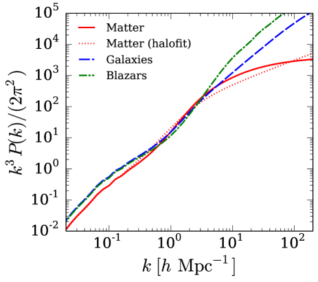
Figure 13: Power spectra of matter (solid), galaxies (dashed), and blazars (dot-dashed) due to halo model at $z=0$. The matter power spectrum due to ‘halofit’ [56] is also shown for comparison (dotted).

We implement the halo model computation by treating central and satellite galaxies separately. The galaxy power spectrum as the result is divided into one-halo and two-halo terms as follows (e.g., [29, 57]):

$$P_{\rm g}(k,z) = P_{\rm g}^{\rm 1h}(k,z)+P_{\rm g}^{\rm 2h}(k,z),$$ (B.5)

$$P_{\rm g}^{\rm 1h}(k,z) = \int dM\frac{dn(M,z)}{dM}\frac{1}{\langle n_{\rm g}(z)\rangle^{2}}\left[2\langle N_{\rm cen}N_{\rm sat}|M\rangle\tilde{u}_{\rm sat}(k|M)\right.$$ (B.6)

$${}\left.+\langle N_{\rm sat}(N_{\rm sat}-1)|M\rangle|\tilde{u}_{\rm sat}(k|M)|^{2}\right],$$

$$P_{\rm g}^{\rm 2h}(k,z) = b_{\rm 1,g}^{2}(z)P_{\rm lin}(k,z),$$ (B.7)

where $\tilde{u}_{\rm sat}(k|M)$ is the Fourier transform of the normalized satellite distribution in a halo with the mass $M$, $u_{\rm sat}(r|M)$, for which we assume the NFW profile, and $b_{1,{\rm g}}$ is the linear bias, for which we adopt 1.4 independent of redshifts [58]. Here we assumed that the central galaxies locate at the center of the host halo, and therefore, the auto-correlation of the central galaxy simply yields a shot noise that is not included here but discussed in Appendix A. The first term of Eq. (B.6) represents the correlation between the central and one of the satellite galaxies, while the second term represents that between two of the satellites. Remembering that $N_{\rm sat}>0$ only if $N_{\rm cen}=1$, we have $\langle N_{\rm cen}N_{\rm sat}|M\rangle=\langle N_{\rm sat}|M\rangle$. Also the HOD of satellite galaxies is well approximated to the Poisson distribution [55], and thus we have $\langle N_{\rm sat}(N_{\rm sat}-1)|M\rangle=\langle N_{\rm sat}|M\rangle^{2}$. With these and Eqs. (B.1)–(B.3), we compute the galaxy power spectrum through Eqs. (B.5)–(B.7).

Figure 13 shows the galaxy power spectrum $P_{\rm g}(k)$ at $z=0$, and the comparison with the matter power spectrum using the same halo model (e.g., [29, 30]) and a ‘halofit’ model [59, 56]. The linear power spectrum as well as the halofit model were computed with the CAMB numerical code. We find substantial deviation of the galaxy power spectrum from that for matter especially at scales smaller than $\sim$0.1 $h^{-1}\,{\rm Mpc}$.

B.2 Blazar-galaxy cross-power spectrum

The HOD for the gamma-ray blazar population is hardly known observationally. It is, however, possible to use the knowledge from other wavebands such as X rays in order to study it. Although clustering properties of X-ray AGNs are certainly less studied compared with those of galaxies, it is found that they selectively live in $\sim$10${}^{13.1}h^{-1}M_{\odot}$ dark matter halos [51, 52]. We here assume that such a property is common for the AGNs that are also bright in gamma rays, and also that such AGNs only reside at the center of the host dark matter halos. With these approximations, we write the blazar-galaxy cross-power spectrum $P_{\rm b,g}(k,z)$ as

$$P_{\rm b,g}(k,z) = P_{\rm b,g}^{\rm 1h}(k,z)+P_{\rm b,g}^{\rm 2h}(k,z),$$ (B.8)

$$P_{\rm b,g}^{\rm 1h}(k,z) = \frac{\langle N_{\rm sat}|M_{\rm b}\rangle}{\langle n_{\rm g}(z)\rangle}\tilde{u}_{\rm sat}(k|M_{\rm b}),$$ (B.9)

$$P_{\rm b,g}^{\rm 2h}(k,z) = b_{1}(M_{\rm b},z)b_{\rm 1,g}(z)P_{\rm lin}(k,z),$$ (B.10)

where $M_{\rm b}=10^{13.1}h^{-1}M_{\odot}$ is the mass of the dark matter halos that host blazars. The one-halo term takes correlation between a central AGN and satellite galaxies, while the correlation with a central galaxy yields shot noise that was treated in Appendix A. The former corresponds to the first term of Eq. (B.6), but divided by 2 and computed with a very sharp mass function, $dn/dM\propto\delta_{\rm D}(M-M_{\rm b})$.

We show the blazar power spectrum in Fig. 13, and find that they cluster even more strongly than galaxies at small scales.

Appendix C Cross correlation between density squared and galaxy distribution

In the halo model, all the dark matter particles are confined in halos. The central position and mass of the halo are represented by $\bm{x}_{i}$ and $M_{i}$, respectively, and the matter density squared is then written as

$$\rho_{\rm m}^{2}(\bm{x})=\int d^{3}x^{\prime}\int dM\sum_{i}\delta_{\rm D}^{3}(\bm{x}^{\prime}-\bm{x}_{i})\delta_{\rm D}(M-M_{i})\mathcal{J}(M,z^{\prime})u_{\delta^{2}}(\bm{x}-\bm{x}^{\prime}|M),$$ (C.1)

where $u_{\delta^{2}}(\bm{x}|M)$ is the profile of density squared of a halo with mass $M$, which is normalized to unity after volume integration. Recalling that the ensemble average of the product of delta functions gives the halo mass function:

$$\left\langle\sum_{i}\delta_{\rm D}^{3}(\bm{x}-\bm{x}_{i})\delta_{\rm D}(M-M_{i})\right\rangle=\frac{dn(M,z)}{dM},$$ (C.2)

we recover Eq. (2.4).

For the number density of the galaxies, instead of using the sum of the delta functions of the coordinates [Eq. (A.1)], we regard galaxies as particles smoothly distributed around the halo at $\bm{x}_{j}$, following $u_{\rm g}$:

$$n_{\rm g}(\bm{x})=\int d^{3}x^{\prime}\int dM\sum_{j}\delta_{\rm D}^{3}(\bm{x}^{\prime}-\bm{x}_{j})\delta_{\rm D}(M-M_{j})N_{\rm g}(M)u_{\rm g}(\bm{x}-\bm{x}^{\prime}|M).$$ (C.3)

Again, by taking the ensemble average, one recovers Eq. (B.4).

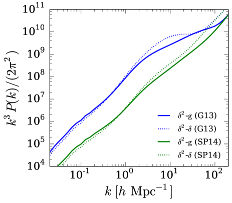
Figure 14: Cross-power spectrum between density squared and galaxy distribution (solid) or density (dotted) at $z=0$. Results for two boost models are shown; [24] for the upper curves (labeled as G13) and [26] for the lower (SP14).

Following the same argument as in Eq. (A.4), the two-point cross-correlation function between $\delta\rho_{\rm m}^{2}=\rho_{\rm m}^{2}-\langle\rho_{\rm m}^{2}\rangle$ and $\delta n_{\rm g}$ is written as

$$\langle\delta\rho_{\rm m}^{2}(\bm{x}_{1})\delta n_{\rm g}(\bm{x}_{2})\rangle \equiv \langle\rho_{\rm m}\rangle^{2}\langle n_{\rm g}(z_{2})\rangle\xi_{\delta^{2},{\rm g}}(\bm{x}_{1}-\bm{x}_{2})$$ (C.4)

$$= \int d^{3}x_{1}^{\prime}\int dM_{1}\frac{dn(M_{1},z_{1})}{dM_{1}}\mathcal{J}(M_{1},z_{1})u_{\delta^{2}}(\bm{x}_{1}-\bm{x}_{1}^{\prime}|M_{1})$$

$${}\times\langle N_{\rm g}|M_{1}\rangle u_{\rm g}(\bm{x}_{2}-\bm{x}_{1}^{\prime}|M_{1})$$

$${}+\int d^{3}x_{1}^{\prime}\int dM_{1}\int d^{3}x_{2}^{\prime}\int dM_{2}\frac{dn(M_{1},z_{1})}{dM_{1}}\frac{dn(M_{2},z_{2})}{dM_{2}}$$

$${}\times\mathcal{J}(M_{1},z_{1})u_{\delta^{2}}(\bm{x}_{1}-\bm{x}_{1}^{\prime}|M_{1})\langle N_{\rm g}|M_{2}\rangle u_{\rm g}(\bm{x}_{2}-\bm{x}_{2}^{\prime}|M_{2})$$

$${}\times\xi_{\rm hh}(\bm{x}_{1}^{\prime}-\bm{x}_{2}^{\prime}|M_{1},M_{2}),$$

where $\xi_{\rm hh}$ is the two-point correlation function of the halo seeds. In the following, we approximate it as $\xi_{\rm hh}(r|M_{1},M_{2})\approx b_{1}(M_{1})b_{2}(M_{2})\xi_{\rm lin}(r)$, where $\xi_{\rm lin}$ is the linear correlation function. The cross-power spectrum, defined as the Fourier transform of $\xi_{\delta^{2},{\rm g}}(r)$ [Eq. (C.4)], is derived, after straightforward algebra, as

$$P_{\delta^{2},{\rm g}}(k,z) = P_{\delta^{2},{\rm g}}^{\rm 1h}(k,z)+P_{\delta^{2},{\rm g}}^{\rm 2h}(k,z),$$ (C.5)

$$P_{\delta^{2},{\rm g}}^{\rm 1h}(k,z) = \int dM\frac{dn(M,z)}{dM}\frac{\mathcal{J}(M,z)}{(\Omega_{\rm m}\rho_{\rm c})^{2}}\frac{\langle N_{\rm g}|M\rangle}{\langle n_{\rm g}(z)\rangle}\tilde{u}_{\delta^{2}}(k|M)\tilde{u}_{\rm g}(k|M),$$ (C.6)

$$P_{\delta^{2},{\rm g}}^{\rm 2h}(k,z) = \left[\int dM\frac{dn(M,z)}{dM}\frac{\mathcal{J}(M,z)}{(\Omega_{\rm m}\rho_{\rm c})^{2}}\tilde{u}_{\delta^{2}}(k|M)b_{1}(M,z)\right]$$ (C.7)

$${}\times\left[\int dM^{\prime}\frac{dn(M^{\prime},z)}{dM^{\prime}}\frac{\langle N_{\rm g}|M^{\prime}\rangle}{\langle n_{\rm g}(z)\rangle}\tilde{u}_{\rm g}(k|M^{\prime})b_{1}(M^{\prime},z)\right]P_{\rm lin}(k,z),$$

where $\tilde{u}_{\delta^{2}}(k)$ is the Fourier transform of $u_{\delta^{2}}(r)$, and

$$\langle N_{\rm g}|M\rangle\tilde{u}_{\rm g}(k|M)=\langle N_{\rm cen}|M\rangle+\langle N_{\rm sat}|M\rangle\tilde{u}_{\rm sat}(k|M).$$ (C.8)

In Fig. 14, we show $P_{\delta^{2},{\rm g}}(k,0)$ for both the boost models [24, 26]. We also compare the results with $P_{\delta^{2},\delta}(k,0)$ within the same framework of the halo model, which was adopted in Ref. [21]. At small scales, $\delta^{2}$-g correlation is smaller even though it is very similar to $\delta^{2}$-$\delta$ power spectrum.

Finally, after projection for which the same procedure is used as in Appendix A, the angular cross-power spectrum between dark matter annihilation and the galaxy distribution is obtained with

$$C_{\ell}^{\rm dm,g}=\int\frac{d\chi}{\chi^{2}}W_{\rm dm}(z)W_{\rm g}(z)P_{\delta^{2},{\rm g}}\left(\frac{\ell}{\chi},z\right).$$ (C.9)

References

- [1] G. Jungman, M. Kamionkowski, and K. Griest, Supersymmetric dark matter, Phys. Rept. 267 (1996) 195–373, [hep-ph/9506380].
- [2] T. Bringmann and C. Weniger, Gamma Ray Signals from Dark Matter: Concepts, Status and Prospects, Phys. Dark Univ. 1 (2012) 194–217, [arXiv:1208.5481].
- [3] S. Ando and E. Komatsu, Anisotropy of the cosmic gamma-ray background from dark matter annihilation, Phys. Rev. D73 (2006) 023521, [astro-ph/0512217].
- [4] S. Ando, E. Komatsu, T. Narumoto, and T. Totani, Dark matter annihilation or unresolved astrophysical sources? Anisotropy probe of the origin of cosmic gamma-ray background, Phys. Rev. D75 (2007) 063519, [astro-ph/0612467].
- [5] F. Miniati, S. M. Koushiappas, and T. Di Matteo, Angular Anisotropies in the Cosmic Gamma-Ray Background as a Probe of Its Origin, Astrophys. J. 667 (2007) L1–L4, [astro-ph/0702083].
- [6] A. Cuoco, J. Brandbyge, S. Hannestad, T. Haugboelle, and G. Miele, Angular Signatures of Annihilating Dark Matter in the Cosmic Gamma-Ray Background, Phys. Rev. D77 (2008) 123518, [arXiv:0710.4136].
- [7] J. M. Siegal-Gaskins, Revealing dark matter substructure with anisotropies in the diffuse gamma-ray background, JCAP 0810 (2008) 040, [arXiv:0807.1328].
- [8] S. K. Lee, S. Ando, and M. Kamionkowski, The Gamma-Ray-Flux Probability Distribution Function from Galactic Halo Substructure, JCAP 0907 (2009) 007, [arXiv:0810.1284].
- [9] M. Fornasa, L. Pieri, G. Bertone, and E. Branchini, Anisotropy probe of galactic and extra-galactic Dark Matter annihilations, Phys. Rev. D80 (2009) 023518, [arXiv:0901.2921].
- [10] S. Ando, Gamma-ray background anisotropy from galactic dark matter substructure, Phys. Rev. D80 (2009) 023520, [arXiv:0903.4685].
- [11] J. Zavala, V. Springel, and M. Boylan-Kolchin, Extragalactic gamma-ray background radiation from dark matter annihilation, Mon. Not. Roy. Astron. Soc. 405 (2010) 593, [arXiv:0908.2428].
- [12] S. Ando and V. Pavlidou, Imprint of Galaxy Clustering in the Cosmic Gamma-Ray Background, Mon. Not. Roy. Astron. Soc. 400 (2009) 2122, [arXiv:0908.3890].
- [13] A. Ibarra, D. Tran, and C. Weniger, Detecting Gamma-Ray Anisotropies from Decaying Dark Matter: Prospects for Fermi LAT, Phys. Rev. D81 (2010) 023529, [arXiv:0909.3514].
- [14] J. M. Siegal-Gaskins, R. Reesman, V. Pavlidou, S. Profumo, and T. P. Walker, Anisotropies in the gamma-ray sky from millisecond pulsars, Mon.Not.Roy.Astron.Soc. 415 (2011) 1074–1082, [arXiv:1011.5501].
- [15] A. Cuoco, A. Sellerholm, J. Conrad, and S. Hannestad, Anisotropies in the diffuse gamma-ray background from dark matter with Fermi LAT: a closer look, Mon. Not. Roy. Astron. Soc. 414 (2011) 2040–2054, [arXiv:1005.0843].
- [16] M. Fornasa, J. Zavala, M. A. Sanchez-Conde, J. M. Siegal-Gaskins, T. Delahaye, et. al., Characterization of Dark-Matter-induced anisotropies in the diffuse gamma-ray background, Mon. Not. Roy. Astron. Soc. 429 (2013) 1529, [arXiv:1207.0502].
- [17] S. Ando and E. Komatsu, Constraints on the annihilation cross section of dark matter particles from anisotropies in the diffuse gamma-ray background measured with Fermi-LAT, Phys. Rev. D87 (2013) 123539, [arXiv:1301.5901].
- [18] M. Ackermann et. al., Anisotropies in the diffuse gamma-ray background measured by the Fermi LAT, Phys. Rev. D85 (2012) 083007, [arXiv:1202.2856].
- [19] A. Cuoco, E. Komatsu, and J. Siegal-Gaskins, Joint anisotropy and source count constraints on the contribution of blazars to the diffuse gamma-ray background, Phys. Rev. D86 (2012) 063004, [arXiv:1202.5309].
- [20] G. Gomez-Vargas et. al., Dark Matter implications of Fermi-LAT measurement of anisotropies in the diffuse gamma-ray background, arXiv:1303.2154.
- [21] S. Ando, A. Benoit-Lévy, and E. Komatsu, Mapping dark matter in the gamma-ray sky with galaxy catalogs, Phys. Rev. D90 (2014) 023514, [arXiv:1312.4403].
- [22] N. Fornengo and M. Regis, Particle dark matter searches in the anisotropic sky, Front. Physics 2 (2014) 6, [arXiv:1312.4835].
- [23] J. P. Huchra, L. M. Macri, K. L. Masters, T. H. Jarrett, P. Berlind, M. Calkins, A. C. Crook, R. Cutri, P. Erdoǧdu, E. Falco, T. George, C. M. Hutcheson, O. Lahav, J. Mader, J. D. Mink, N. Martimbeau, S. Schneider, M. Skrutskie, S. Tokarz, and M. Westover, The 2MASS Redshift Survey — Description and Data Release, Astrophys. J. Suppl. Ser. 199 (2012) 26, [arXiv:1108.0669].
- [24] L. Gao, C. Frenk, A. Jenkins, V. Springel, and S. White, Where will supersymmetric dark matter first be seen?, Mon. Not. Roy. Astron. Soc. 419 (2012) 1721, [arXiv:1107.1916].
- [25] G. Steigman, B. Dasgupta, and J. F. Beacom, Precise Relic WIMP Abundance and its Impact on Searches for Dark Matter Annihilation, Phys.Rev. D86 (2012) 023506, [arXiv:1204.3622].
- [26] M. A. Sanchez-Conde and F. Prada, The flattening of the concentration-mass relation towards low halo masses and its implications for the annihilation signal boost, Mon. Not. Roy. Astron. Soc. 442 (2014) 2271, [arXiv:1312.1729].
- [27] S. Camera, M. Fornasa, N. Fornengo, and M. Regis, A Novel Approach in the Weakly Interacting Massive Particle Quest: Cross-correlation of Gamma-Ray Anisotropies and Cosmic Shear, Astrophys.J. 771 (2013) L5, [arXiv:1212.5018].
- [28] R. Trotta, Bayes in the sky: Bayesian inference and model selection in cosmology, Contemp.Phys. 49 (2008) 71–104, [arXiv:0803.4089].
- [29] U. Seljak, Analytic model for galaxy and dark matter clustering, Mon. Not. Roy. Astron. Soc. 318 (2000) 203, [astro-ph/0001493].
- [30] A. Cooray and R. K. Sheth, Halo models of large scale structure, Phys. Rept. 372 (2002) 1–129, [astro-ph/0206508].
- [31] R. C. Gilmore, R. S. Somerville, J. R. Primack, and A. Domínguez, Semi-analytic modelling of the extragalactic background light and consequences for extragalactic gamma-ray spectra, Mon. Not. Roy. Astron. Soc. 422 (2012) 3189–3207, [arXiv:1104.0671].
- [32] A. A. Klypin, A. V. Kravtsov, O. Valenzuela, and F. Prada, Where are the missing Galactic satellites?, Astrophys. J. 522 (1999) 82–92, [astro-ph/9901240].
- [33] B. Moore, S. Ghigna, F. Governato, G. Lake, T. R. Quinn, et. al., Dark matter substructure within galactic halos, Astrophys. J. 524 (1999) L19–L22, [astro-ph/9907411].
- [34] J. F. Navarro, C. S. Frenk, and S. D. White, A Universal density profile from hierarchical clustering, Astrophys. J. 490 (1997) 493–508, [astro-ph/9611107].
- [35] R. K. Sheth and G. Tormen, Large scale bias and the peak background split, Mon. Not. Roy. Astron. Soc. 308 (1999) 119, [astro-ph/9901122].
- [36] A. Abdo et. al., The Spectrum of the Isotropic Diffuse Gamma-Ray Emission Derived From First-Year Fermi Large Area Telescope Data, Phys. Rev. Lett. 104 (2010) 101101, [arXiv:1002.3603].
- [37] M. Di Mauro, F. Calore, F. Donato, M. Ajello, and L. Latronico, Diffuse -Ray Emission from Misaligned Active Galactic Nuclei, Astrophys. J. 780 (2014) 161, [arXiv:1305.4200].
- [38] M. Ajello, M. S. Shaw, R. W. Romani, C. D. Dermer, L. Costamante, O. G. King, W. Max-Moerbeck, A. Readhead, A. Reimer, J. L. Richards, and M. Stevenson, The Luminosity Function of Fermi-detected Flat-spectrum Radio Quasars, Astrophys. J. 751 (2012) 108, [arXiv:1110.3787].
- [39] M. Ajello, R. W. Romani, D. Gasparrini, M. S. Shaw, J. Bolmer, G. Cotter, J. Finke, J. Greiner, S. E. Healey, O. King, W. Max-Moerbeck, P. F. Michelson, W. J. Potter, A. Rau, A. C. S. Readhead, J. L. Richards, and P. Schady, The Cosmic Evolution of Fermi BL Lacertae Objects, Astrophys. J. 780 (2014) 73, [arXiv:1310.0006].
- [40] A. A. Abdo et. al., The First Catalog of Active Galactic Nuclei Detected by the Fermi Large Area Telescope, Astrophys. J. 715 (2010) 429–457, [arXiv:1002.0150].
- [41] A. A. Abdo et. al., The Fermi-LAT High-Latitude Survey: Source Count Distributions and the Origin of the Extragalactic Diffuse Background, Astrophys. J. 720 (2010) 435–453, [arXiv:1003.0895].
- [42] C. Gruppioni et. al., The Herschel PEP/HerMES luminosity function - I. Probing the evolution of PACS selected Galaxies to z 4, Mon. Not. Roy. Astron. Soc. 432 (2013) 23–52, [arXiv:1302.5209].
- [43] I. Tamborra, S. Ando, and K. Murase, Star-forming galaxies as the origin of diffuse high-energy backgrounds: Gamma-ray and neutrino connections, and implications for starburst history, arXiv:1404.1189.
- [44] M. Ackermann et. al., GeV Observations of Star-forming Galaxies with Fermi LAT, Astrophys. J. 755 (2012) 164, [arXiv:1206.1346].
- [45] E. Branchini, M. Davis, and A. Nusser, The linear velocity field of 2MASS Redshift Survey, Ks= 11.75 galaxies: constraints on and bulk flow from the luminosity function, Mon. Not. Roy. Astron. Soc. 424 (2012) 472–481, [arXiv:1202.5206].
- [46] T. Jarrett, Large scale structure in the local universe: the 2mass galaxy catalog, Publ. Astron. Soc. Austral. 21 (2004) 396–403, [astro-ph/0405069].
- [47] T.-H. Jarrett, T. Chester, R. Cutri, S. Schneider, J. Rosenberg, J. P. Huchra, and J. Mader, 2MASS Extended Sources in the Zone of Avoidance, Astron. J. 120 (2000) 298–313, [astro-ph/0005017].
- [48] J.-Q. Xia, A. Cuoco, E. Branchini, M. Fornasa, and M. Viel, A cross-correlation study of the Fermi-LAT -ray diffuse extragalactic signal, Mon. Not. Roy. Astron. Soc. 416 (2011) 2247–2264, [arXiv:1103.4861].
- [49] R. J. Scherrer and E. Bertschinger, Statistics of primordial density perturbations from discrete seed masses, Astrophys. J. 381 (1991) 349–360.
- [50] J. Han, C. S. Frenk, V. R. Eke, L. Gao, S. D. M. White, A. Boyarsky, D. Malyshev, and O. Ruchayskiy, Constraining extended gamma-ray emission from galaxy clusters, Mon. Not. Roy. Astron. Soc. 427 (2012) 1651–1665, [arXiv:1207.6749].
- [51] V. Allevato, A. Finoguenov, N. Cappelluti, T. Miyaji, G. Hasinger, M. Salvato, M. Brusa, R. Gilli, G. Zamorani, F. Shankar, J. B. James, H. J. McCracken, A. Bongiorno, A. Merloni, J. A. Peacock, J. Silverman, and A. Comastri, The XMM-Newton Wide Field Survey in the COSMOS Field: Redshift Evolution of AGN Bias and Subdominant Role of Mergers in Triggering Moderate-luminosity AGNs at Redshifts up to 2.2, Astrophys. J. 736 (2011) 99, [arXiv:1105.0520].
- [52] N. Cappelluti, V. Allevato, and A. Finoguenov, Clustering of X-Ray-Selected AGN, Adv. Astron. 2012 (2012) 853701, [arXiv:1201.3920].
- [53] M. Tristram, J. Macias-Perez, C. Renault, and D. Santos, Xspect, estimation of the angular power spectrum by computing cross power spectra, Mon. Not. Roy. Astron. Soc. 358 (2005) 833, [astro-ph/0405575].
- [54] M. Bilicki, T. H. Jarrett, J. A. Peacock, M. E. Cluver, and L. Steward, Two Micron All Sky Survey Photometric Redshift Catalog: A Comprehensive Three-dimensional Census of the Whole Sky, Astrophys. J. Suppl. Ser. 210 (2014) 9, [arXiv:1311.5246].
- [55] Z. Zheng, A. A. Berlind, D. H. Weinberg, A. J. Benson, C. M. Baugh, et. al., Theoretical models of the halo occupation distribution: Separating central and satellite galaxies, Astrophys. J. 633 (2005) 791–809, [astro-ph/0408564].
- [56] R. Takahashi, M. Sato, T. Nishimichi, A. Taruya, and M. Oguri, Revising the Halofit Model for the Nonlinear Matter Power Spectrum, Astrophys. J. 761 (2012) 152, [arXiv:1208.2701].
- [57] R. K. Sheth and B. Jain, Substructure and the halo model of large scale structure, Mon. Not. Roy. Astron. Soc. 345 (2003) 529, [astro-ph/0208353].
- [58] M. Davis, A. Nusser, K. L. Masters, C. Springob, J. P. Huchra, and G. Lemson, Local gravity versus local velocity: solutions for and non-linear bias, Mon. Not. Roy. Astron. Soc. 413 (2011) 2906–2922, [arXiv:1011.3114].
- [59] R. Smith et. al., Stable clustering, the halo model and nonlinear cosmological power spectra, Mon. Not. Roy. Astron. Soc. 341 (2003) 1311, [astro-ph/0207664].