Walking dynamics are symmetric (enough)

Abstract

Many biological phenomena such as locomotion, circadian cycles, and breathing are rhythmic in nature and can be modeled as rhythmic dynamical systems. Dynamical systems modeling often involves neglecting certain characteristics of a physical system as a modeling convenience. For example, human locomotion is frequently treated as symmetric about the sagittal plane. In this work, we test this assumption by examining human walking dynamics around the steady-state (limit-cycle). Here we adapt statistical cross validation in order to examine whether there are statistically significant asymmetries, and even if so, test the consequences of assuming bilateral symmetry anyway. Indeed, we identify significant asymmetries in the dynamics of human walking, but nevertheless show that ignoring these asymmetries results in a more consistent and predictive model. In general, neglecting evident characteristics of a system can be more than a modeling convenience—it can produce a better model.

I INTRODUCTION

The concept of symmetry has helped shape our understanding of engineering and biology alike. The Roman text “De architechura” by Vitruvius and the eponymous “Vitruvian Man” by Leornado Da Vinci exemplify the influence of symmetry in animals and humans on man-made works of art and engineering. Symmetry serves to simplify and reduce model complexity, making it a powerful tool in computational and analytical applications. The ubiquity of bilateral (left–right, sagittal plane) symmetry in animals is genetically encoded [1], and from an engineering point of view, building machines with bilateral symmetry is justified by the fact that the left–right axis is unbiased either by gravity or by direction of movement. However, genetic encoding of symmetry manifests itself imperfectly; numerous factors, such as differences in contralateral limb lengths, dominance of “leggedness” and handedness, and developmental processes break perfect symmetry and enhance asymmetry.

Various measures and indices of asymmetry have been used to argue that human locomotion is bilaterally symmetric or asymmetric (for reviews, see [2, 3]). Symmetry is thought to confer some advantages on motor abilities (e.g. improved energetic efficiency [4, 5, 6]). The common trend among previous work is the comparison of kinetic and/or kinematic gait parameters between the right and left halves of the body, i.e. joint angles [7, 8, 9, 10], ranges [11, 12] and velocities [13], stride lengths [14, 15, 12, 10], ground reaction forces [16, 17, 18, 19], EMG profiles [20, 21, 22, 23], limbs forces and moments [24, 25, 26, 27], or center-of-mass oscillations [28, 29, 30]. However, as Sadeghi et. al. [2] state, “…can we argue that it is acceptable to conclude that able-bodied gait is asymmetrical just because of the existence of statistically significant differences between two corresponding parameters (which we call local asymmetry) calculated from the right and left limbs?” During human walking, do steps from left-to-right and right-to-left recover significantly differently from perturbations? After all, there are differences in leg dominance—e.g. preferred kicking leg—that might lead to different responses from step-to-step.

Aside from demonstrating asymmetry (or not) in gait parameters, we found no studies examining the potential benefits of neglecting evident asymmetries. If there is a step-to-step dynamical asymmetry, does fitting a model from stride to stride (two step) rather than step to step (one step) better capture the dynamics of human walking? Of course, no single physical system has perfect symmetry. Thus symmetric models are inherently wrong for any physical system, but may nevertheless be useful for simplifying both the modeling and analysis.

“Essentially all models are wrong, but some are useful” wrote George E. P. Box in his seminal book [31]. According to Box, the important practical concern regarding the models of physical phenomena is “how wrong do they have to be to not be useful?” With regard to bilateral asymmetry in human walking, we attempt to frame this concern as follows. How wrong is it to neglect asymmetry from a statistical point of view? And how useful is symmetric modeling in terms of predictive power and simplicity? In most cases, correctness and usefulness are directly related, and they are tested simultaneously. However, in the context of data-driven modeling of human walking dynamics, the “wrongness” and “usefulness” of assuming symmetry are related but have critical, nuanced differences. The methods presented in this paper allows us to independently (statistically) address these differences.

In this paper, we test the assumption of bilateral symmetry in the dynamics of human walking. As an example, consider fitting linear models to two distinct data sets (e.g. “left steps” and “right steps”) and testing these models in terms of their respective ability to predict isolated validation data from just the one of the data sets, say “left steps”. If walking were perfectly symmetric, both the left-step (“correct”) model and right-step (“wrong”) model would perform indistinguishably in left-step validation. However, we show that there are statistically significant asymmetries in the dynamics of human walking in healthy subjects in the sense that the “wrong” model performs statistically worse than the “correct” model in validation. Despite these asymmetries, we also show that a more consistent and predictive model of the dynamics is obtained by assuming symmetry, and pooling all the data from both left and right steps to form a generic model. Quite surprisingly, this fit significantly out-performs the mapping fitted to only left steps even when predicting left-step data. This is good news because, in addition to our finding that it is statistically better to neglect asymmetry, it is also practically and theoretically convenient to assume symmetry. These advantages lead us to conclude that the assumption of symmetry in walking dynamics, though clearly wrong in a platonic sense, is nevertheless more useful for all practical purposes.

I-A Modeling the Rhythmic Dynamics

Our approach to analyzing and modeling walking involves treating the underlying behavior as a finite-dimensional nonlinear rhythmic dynamical system operating around a stable limit cycle. This type of modeling approach has been successful for robotic [32, 33, 34, 35] and biological systems [36, 37, 38, 39, 40]. A limit cycle is an isolated periodic trajectory that is a solution to the equations governing the dynamical system [41]. A limit cycle is said to be stable if all trajectories in a sufficiently small neighborhood of the limit cycle converge to it.

We further use Poincaré theory in our analysis of rhythmic walking dynamics. A Poincaré return map [41, 38] is a mapping from a transverse section $S$ back to itself, obtained by tracing the consecutive intersections of the state trajectories with the section $S$. This return map reduces the continuous rhythmic dynamical system to a nonlinear discrete dynamical system that preserves many properties of the behavior. The specific Poincaré section that we adopt for human walking is the heel strike event, as explained in Section II-B.

The intersection of the limit cycle with the Poincaré section is an isolated fixed point of the return map. The limit cycle is asymptotically stable if and only if this fixed point is stable. Our second modeling approximation is based on the Hartman–-Grobman theorem (or linearization theorem), which states that local flow around any hyperbolic fixed point is homeomorphic to the one governed by its linearization around the fixed point itself. Thus as detailed in Section II-B, we fit linear models to walking trajectories on the Poincaré maps.

I-B Limit-Cycle Dynamics and Symmetry

Here, we define symmetry in the context of limit-cycle modeling of walking and consider what kind of symmetries (and asymmetries) can be addressed using this approach.

In our modeling approach, there are two core elements: the limit-cycle of the rhythmic system, which characterizes the steady-state behavior, and the dynamics (both deterministic and stochastic) around the limit-cycle. In this paper, we are interested in the latter.

Beyond its utility for approximation, bilateral symmetry of the (steady-state) limit-cycle trajectory may have physiological significance, such as reducing metabolic cost [6, 4, 5]. Indeed, the kinematic and kinetic variables that are the focus of the majority of studies that address human [2] or animal [42, 43] locomotor symmetry are steady-state (periodic) variables that correspond to the limit cycle of a dynamic model.

Here, we consider the dynamics near, but off of the limit cycle, using data from Poincaré sections to estimate return maps. Hence our analysis is not based on the steady-state parameters of gait, but how the gait deviates from and recovers to these steady-state parameters. To the best of our knowledge, this is the first study that analyzes the dynamical symmetry of biological rhythmic systems. We validate our methods in data from normal human walking experiments. These methods are also applicable to robotic or biological locomotor behavior with approximately symmetric gait patterns.

II METHODS

The system of interest is human treadmill walking. This data set is obtained for eight healthy young adult participants, at three different belt speeds (0.5, 1.0, and 1.5 m/s). We required the subjects to cross their arms in order to continuously record the marker positions. The Johns Hopkins Institutional Review Board approved all protocols and all subjects gave informed written consent prior to participation.

II-A Kinematic Data

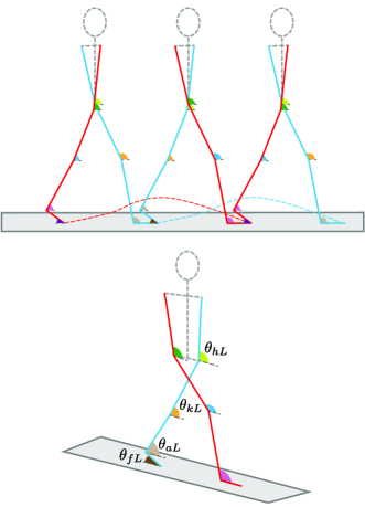
Figure 1: Visualization of leg angle vector $\bm{\theta}$. The left leg (blue) and right leg (red) alternate between stance and swing phase over the course of a stride. The variables $\theta_{fL}$, $\theta_{aL}$, $\theta_{kL}$, and $\theta_{hL}$ correspond to the left foot, ankle, knee, and hip angles respectively. The corresponding right leg angles, $\theta_{fR}$, $\theta_{aR}$, $\theta_{kR}$, and $\theta_{hR}$, are not labeled. The $8$ leg angles and their respective angular velocities form the $16$-dimensional state vector.

We placed infrared (IR) markers on subjects’ left and right shoulder, hip, knee, ankle, and toe. Markers were tracked in 3D using Optotrak (Northern Digital) at 100 Hz. The marker data were used to calculate the four sagittal plane angles on each side as illustrated in Figure 1. The raw angular data were smoothed with a fifth-order, zero-phase-lag (non-causal) Butterworth filter ($5^{th}$ order with a cut-off frequency of $10\mathrm{Hz}$) to remove measurement noise and ease angular velocity estimation. In order to estimate angular velocities, a central difference filter and another zero-phase-lag Butterworth filter was applied to the smoothed angular data similar to the methods adopted in the biomechanics literature [44, 45]. We assume that the smoothed angles (8) and angular velocities (8) form a 16 dimensional state space for walking. The state vector includes angles (rad),

$$\bm{\theta_{L}}(t) =\begin{bmatrix}\theta_{fL}&\theta_{aL}&\theta_{kL}&\theta_{hL}\end{bmatrix}^{T},$$ (1)

$$\bm{\theta_{R}}(t) =\begin{bmatrix}\theta_{fR}&\theta_{aR}&\theta_{kR}&\theta_{hR}\end{bmatrix}^{T},$$

$$\bm{\theta}(t) =\begin{bmatrix}\bm{\theta_{L}}(t)\\ \bm{\theta_{R}}(t)\end{bmatrix}$$

and angular velocities (rad/s),

$$\dot{\bm{\theta}}_{\bm{L}}(t) =\begin{bmatrix}\dot{\theta}_{fL}&\dot{\theta}_{aL}&\dot{\theta}_{kL}&\dot{\theta}_{hL}\end{bmatrix}^{T},$$ (2)

$$\dot{\bm{\theta}}_{\bm{R}}(t) =\begin{bmatrix}\dot{\theta}_{fR}&\dot{\theta}_{aR}&\dot{\theta}_{kR}&\dot{\theta}_{hR}\end{bmatrix}^{T},$$

$$\dot{\bm{\theta}}(t) =\begin{bmatrix}\dot{\bm{\theta}}_{\bm{L}}(t)\\ \dot{\bm{\theta}}_{\bm{R}}(t)\end{bmatrix}.$$

Subscripts $f$, $a$, $k$, and $h$ stand for foot, ankle, knee, and hip, respectively. $L$ and $R$ mnemonically denote the left and right legs.

In order to analyze the data independently from the physical units, the state space was non-dimensionalized based on the time constant associated with pendular walking [46, 47, 48, 49]:

$$\bar{\bm{\theta}} =\bm{\theta}$$ (3)

$$\bar{\dot{\bm{\theta}}} =\dot{\bm{\theta}}\sqrt{\frac{l_{0}}{g}},$$

where the bar represents the corresponding non-dimensionalized variable, $g$ is the gravitational acceleration, and $l_{0}$ is the leg length of the subject, which is estimated from the marker positions on right hip and ankle.

II-B Events and Section Data

The treadmill used in this study features a split belt that mechanically decouples the vertical ground reaction forces caused by each foot. Each belt is instrumented with a separate load cell, facilitating the estimation of the timing of heel-strike events. We chose heel-strike events as Poincaré sections for the analyses.

Let $t[k]$ be the detected times of heel-strike events, where $k\in\mathcal{K}=\{1,2,3,\dots,k_{\mathrm{max}}\}$, with $k_{\mathrm{max}}$ being the total number of heel-strike events of both legs in one walking trial. For example, if the first heel-strike event ($k=1$) corresponds to the left leg, sets of odd ($\mathcal{K}_{L}$) and even ($\mathcal{K}_{R}$) integer indices from 1 to $k_{\mathrm{max}}$ correspond to the left and right heel-strike events, respectively, such that $\mathcal{K}=\mathcal{K}_{L}\cup\mathcal{K}_{R}$. Over one stride of walking, there are two Poincaré sections of interest at heel-strike events. The measurement of the state vector at these Poincaré sections is given as follows:

$$\textbf{z}[k]=\begin{bmatrix}\bar{\bm{\theta}}(t[k])\\ \bar{\dot{\bm{\theta}}}(t[k])\end{bmatrix}.$$ (4)

During steady-state walking and in the absence of noise, the periodic orbit would remain on the limit cycle:

$$\bm{z}[m] =\bm{\mu}_{L}\ ,\ \forall m\in\mathcal{K}_{L}$$ (5)

$$\bm{z}[m^{\prime}] =\bm{\mu}_{R}\ ,\ \forall m^{\prime}\in\mathcal{K}_{R}$$

where $\bm{\mu}_{L}$ and $\bm{\mu}_{R}$ are the fixed-points with respect to each of the two distinct Poincaré sections. Note that assuming bilateral symmetry implies that these two fixed points are identical up to a relabeling [50, 33, 51, 52]. This relabeling can be expressed as a linear mapping of right-heel-strike coordinates:

$$M:\begin{bmatrix}\bar{\bm{\theta}}_{L}(t[k])\\ \bar{\bm{\theta}}_{R}(t[k])\\ \bar{\dot{\bm{\theta}}}_{L}(t[k])\\ \bar{\dot{\bm{\theta}}}_{R}(t[k])\end{bmatrix}\mapsto\begin{bmatrix}\bar{\bm{\theta}}_{R}(t[k])\\ \bar{\bm{\theta}}_{L}(t[k])\\ \bar{\dot{\bm{\theta}}}_{R}(t[k])\\ \bar{\dot{\bm{\theta}}}_{L}(t[k])\end{bmatrix},\ \forall k\in\mathcal{K}_{R},$$ (6)

where

$$M=\begin{bmatrix}0&I_{4\times 4}&0&0\\ I_{4\times 4}&0&0&0\\ 0&0&0&I_{4\times 4}\\ 0&0&I_{4\times 4}&0\\ \end{bmatrix}.$$ (7)

As explained in Section I-A our approach to modeling human walking centers around fitting linear maps between Poincaré sections around the associated fixed points. First, we estimated the fixed points via

$$\hat{\bm{\mu}}_{L} =\frac{1}{|\mathcal{K}_{L}|}\sum\limits_{k\in\mathcal{K}_{L}}\bm{z}[k],$$ (8)

$$\hat{\bm{\mu}}_{R} =\frac{1}{|\mathcal{K}_{R}|}\sum\limits_{k\in\mathcal{K}_{R}}\bm{z}[k],$$

where $|\mathcal{K}_{L}|$ and $|\mathcal{K}_{R}|$ denote the cardinality of sets $\mathcal{K}_{L}$ and $\mathcal{K}_{R}$ respectively. Note that kinematic asymmetry could be measured directly in terms of the difference between respective fixed points $\hat{\bm{\mu}}_{L}$ and $\hat{\bm{\mu}}_{L}$. While potentially of interest, the current paper focuses on dynamical asymmetry (measured in terms of the section maps), and thus we computed the residuals by subtracting the estimated fixed points from the section data:

$$\bm{q}_{L}[k] =\bm{z}[k]-\hat{\bm{\mu}}_{L}, k\in\mathcal{K}_{L},$$ (9)

$$\bm{q}_{R}[k] =\bm{z}[k]-\hat{\bm{\mu}}_{R}, k\in\mathcal{K}_{R}.$$

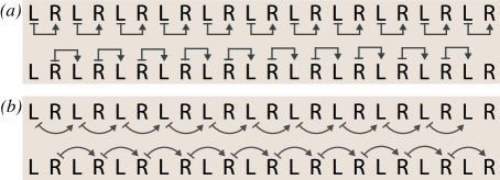
Figure 2: Types of input–output pairs analyzed in this paper. $L$ and $R$ represent the Poincaré sections associated with heel-strike events of the left and right legs. (a) Left-to-right step maps (top) and right-to-left step maps (bottom). Step maps are denoted using straight arrows. (b) Left-to-left stride maps (top) and right-to-right stride maps (bottom). Stride maps and step maps are distinguished throughout the paper by shape (straight versus curved arrows, respectively).

Section maps were estimated using these residuals. A section map from $\bm{q}_{L}$ to the subsequent $\bm{q}_{R}$ is denoted as $L\mapsto R$. We fit two categories of section maps: step-to-step ($L\mapsto R$ and $R\mapsto L$) and stride-to-stride ($L\mapsto L$ and $R\mapsto R$). These sections maps are illustrated in Figure 2(a).

II-C Fitting Section Maps

To fit the section maps for each category explained above, we stack all the appropriate residuals ($\bm{q}_{L}$ and/or $\bm{q}_{R}$) in matrices $X$ (input) and $Y$ (output):

$$X=[x_{1},\cdots,x_{N}]^{T},\ Y=[y_{1},\cdots,y_{N}]^{T},\ x_{i},y_{i}\in\mathbb{R}^{d},$$ (10)

where $x_{i}$ and $y_{i}$ represent residuals ($\bm{q}$) from sections evaluated in the data. For example, to fit the $L\mapsto R$ step-to-step map, one would set the columns of $X$ and $Y$ as follows:

$$x_{1} =q_{L}[1], y_{1} =q_{R}[2],$$ (11)

$$x_{2} =q_{L}[3], y_{2} =q_{R}[4],$$

$$\,\vdots \,\vdots$$

$$x_{N} =q_{L}[2N-1], y_{N} =q_{R}[2N].$$

The linear section maps are modeled as $y_{i}=Ax_{i}+\delta_{i},\ \forall i$, where $\delta_{i}$ is additive noise. The section map can be estimated via least squares:

$$\hat{A}=\left(X^{\dagger}Y\right)^{T}.$$ (12)

where $X^{\dagger}$ is the Moore-–Penrose pseudoinverse of $X$.

III STATISTICAL APPROACH

Here, we tailor Monte-Carlo cross validation to examine symmetry in walking dynamics. (A similar technique based on bootstrap sampling produces qualitatively similar results [53].)

III-A Test of Symmetry Using Monte Carlo Cross-Validation

Classical cross validation (CV) involves fitting a model to a training set of input–output data and validating the model by comparing its predictions on a complementary test set of input–output data. In classical CV, there are $n$ pairs of input–output data which are then split into a training (fitting) set ($n_{f}$ pairs) and complementary test (validation) set ($n_{v}=n-n_{f}$ pairs). The training set is used for model fitting. The fitted model is then applied to the inputs of the test set to generate output predictions; the error metric between the predicted and actual outputs is the cross-validation error (CVE). The CVE is used to evaluate the performance of the model. CV methods are commonly used for selecting models based on their predictive ability [54, 55, 56, 57]. A review by Arlot and Celisse [58] summarizes different cross-validation methods and discusses their advantages and limitations.

The method that we present in this paper is based on Monte-Carlo cross validation (MCCV) [54]. MCCV randomly splits the data $m$ times with fixed $n_{f}$ and $n_{v}$ (size of training and test sets respectively) over the $m$ iterations. For each iteration, the CVE is computed using the respective training and test sets; the overall CVE is estimated using the mean of these $m$ CVEs.

As mentioned before, the model being fit to input–output data in our case is a linear map. Suppose there are $n$ pairs of input–output data, $(x_{i},y_{i})$, where $i\in\mathcal{I}=\{1,2,3,\dots,n\}$. Split this data into a training set $\mathcal{F}\ni(x_{f},y_{f})$ comprising $n_{f}$ pairs, and test set $\mathcal{V}\ni(x_{v},y_{v})$ comprising $n_{v}$ pairs. Define $X_{\mathcal{F}}$ as the matrix whose rows are $x_{f}^{T}$, and define $Y_{\mathcal{F}}$, $X_{\mathcal{V}}$, and $Y_{\mathcal{V}}$ similarly. We use the following definition of CVE from $\mathcal{F}$ to $\mathcal{V}$:

$$\mathrm{CVE}_{\mathcal{F}\mapsto\mathcal{V}}:=\frac{||Y_{\mathcal{V}}-X_{\mathcal{V}}A_{\mathcal{F}}^{T}||^{2}}{||Y_{\mathcal{V}}||^{2}}$$ (13)

where $||\cdot||$ denotes the Frobenius norm and

$$A_{\mathcal{F}}:=\left(X_{\mathcal{F}}^{\dagger}Y_{\mathcal{F}}\right)^{T}$$ (14)

is the least-squares solution (12) given the training data $\mathcal{F}$.

We tailor classical Monte Carlo CV for systems that may exhibit discrete symmetry. We focus our discussion and notation on human walking, but these methods are applicable to other forms of locomotion that involve nearly bilaterally symmetric gaits, e.g. walking and trotting [49], but not clearly asymmetric gaits, e.g. galloping [59]. In classical Monte Carlo CV, at each iteration, one CVE is computed using (13), where as in our CV method we compute three types of CVEs. Each CVE computation uses the same test set, but the models are fit using three different training sets.

Each application of extended CV method requires a “normal” set, $\mathcal{N}$, and an equal size “mirrored” set, $\mathcal{M}$. In this paper, we analyze four different $(\mathcal{N},\mathcal{M})$ pairs, which are generated using the input–output data types illustrated in Figure 2, i.e. step-to-step transitions ($\{L\mapsto R\}$ and $\{R\mapsto L\}$) and stride-to-stride transitions ($\{L\mapsto L\}$ and $\{R\mapsto R\}$). For example, if the normal data set comprises the left-to-right step transitions, $\mathcal{N}=\{L\mapsto R\}$, the associated mirrored dataset is $\mathcal{M}=\{R\mapsto L\}$. Similarly, for strides, if $\mathcal{N}=\{L\mapsto L\}$ represents the set of all transitions from left heel strike to the subsequent left heel strike, then $\mathcal{M}=\{R\mapsto R\}$ are the corresponding right-to-right transitions. All $(\mathcal{N},\mathcal{M})$ combinations are listed in Table I.

The normal and mirrored sets each include $n$ mutually exclusive input–output pairs, denoted by $(x_{i},y_{i})\in\mathcal{N}$ and $(\hat{x}_{i},\hat{y}_{i})\in\mathcal{M}$, respectively where $i\in\mathcal{I}=\{1,2,\cdots,n\}$. Each iteration of extended CV randomly splits this index set $\mathcal{I}$ into a training index set $\mathcal{I}_{f}$ and test index set $\mathcal{I}_{v}$ in a manner identical to classical CV: $\mathcal{I}_{f}\cup\mathcal{I}_{v}=\mathcal{I}$ and $\mathcal{I}_{f}\cap\mathcal{I}_{v}=\emptyset$. The three types of CVE computations described below draw the test set from the normal dataset:

$$\mathcal{V} =\{(x_{v},y_{v})\in\mathcal{N}\,|\,v\in\mathcal{I}_{v}\}.$$ (15)

Normal Cross Validation (NCV) is the same as classical Monte Carlo CV, in that the training data are also drawn from $\mathcal{N}$:

$$\mathcal{F}_{\mathrm{NCV}} =\{(x_{f},y_{f})\in\mathcal{N}\,|\,f\in\mathcal{I}_{f}\}.$$ (16)

This set is used for fitting the linear model $A_{\mathcal{F}_{\mathrm{NCV}}}$ using (14). Given $A_{\mathcal{F}_{\mathrm{NCV}}}$, the CVE is computed on the common test set $\mathcal{V}$ using (13). For NCV, the mirrored data set $\mathcal{M}$ is not used.

Mirrored Cross Validation (MCV) draws the training data from the mirrored dataset $\mathcal{M}$, using the same training index set $\mathcal{I}_{f}$ as NCV:

$$\mathcal{F}_{\mathrm{MCV}} =\{(\hat{x}_{f},\hat{y}_{f})\in\mathcal{M}\,|\,f\in\mathcal{I}_{f}\}.$$ (17)

As before, this set is used for computing the linear model $A_{\mathcal{F}_{\mathrm{MCV}}}$ using (14). The common test set $\mathcal{V}$ is used for computing the CVE. In MCV, we are using the “wrong” training data (mirrored), which will be critical to detect dynamical asymmetry in walking. Note that the size (and in fact the indices) of the training data in both MCV and NCV are the same.

Combined Cross Validation (CCV) uses training data that is the union of the training sets from NCV and MCV:

$$\mathcal{F}_{\mathrm{CCV}} =\mathcal{F}_{\mathrm{NCV}}\cup\mathcal{F}_{\mathrm{MCV}}.$$ (18)

And, as before, this data subset is used to fit the linear model $A_{\mathcal{F}_{\mathrm{CCV}}}$ and the common test set $\mathcal{V}$ is used for calculating the CVE. Thus the model is fitted on data pooled from both $\mathcal{N}$ and $\mathcal{M}$, while the test data remain the same. Note that CCV uses twice as much data for fitting as either NCV or MCV.

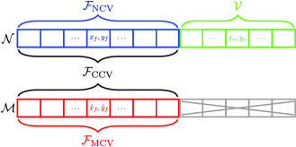
Figure 3: Illustration of the subsets $\mathcal{V}$, $\mathcal{F}_{\mathrm{NCV}}$, $\mathcal{F}_{\mathrm{MCV}}$, and $\mathcal{F}_{\mathrm{CCV}}$ after random splitting during an iteration of extended cross validation methods. The normal dataset, $\mathcal{N}$, is randomly split into the normal training set $\mathcal{F}_{\mathrm{NCV}}$ and the common test set $\mathcal{V}$. $\mathcal{F}_{\mathrm{MCV}}$ shares the same indices as $\mathcal{F}_{\mathrm{NCV}}$ but is drawn from the mirrored dataset, $\mathcal{M}$. The training set for the CCV is simply the union of the other two training sets: $\mathcal{F}_{\mathrm{CCV}}=\mathcal{F}_{\mathrm{NCV}}\cup\mathcal{F}_{\mathrm{MCV}}$. Note that the subset $\mathcal{M}\setminus\mathcal{F}_{\mathrm{MCV}}$ (greyed out) is not used in any of the three CV computations.

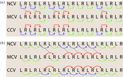
Figure 4: Illustration of extended CV dataset partitioning. (a) For step-to-step data, the normal dataset ($\mathcal{N}$) comprises all left-to-right step ordered pairs, whereas the mirrored dataset ($\mathcal{M}$) comprises all right-to-left step ordered pairs. (b) For stride-to-stride data, the normal dataset ($\mathcal{N}$) comprises all left-to-left stride ordered pairs, whereas the mirrored dataset ($\mathcal{M}$) comprises all right-to-right stride ordered pairs. In both cases, for each iteration, a common test set ($\mathcal{V}$, green arrows), used for all CV methods, is randomly sampled from the normal dataset. The training sets, however, are unique to each method. NCV: the remainder of the normal dataset is used for training ($\mathcal{F}_{\mathrm{NCV}}$, blue arrows). MCV: the training set ($\mathcal{F}_{\mathrm{MCV}}$, red arrows) is obtained using the same indices (dashed lines) as for $\mathcal{F}_{\mathrm{NCV}}$. CCV: the union of the test sets for NCV and MCV, comprise the combined training data ($\mathcal{F}_{\mathrm{CCV}}=\mathcal{F}_{\mathrm{NCV}}\cup\mathcal{F}_{\mathrm{MCV}}$, red and blue arrows).

Figure 3 illustrates the set partitioning for one iteration of extended cross validation for a general dataset. Figure 4(a) illustrates one iteration of the extended cross validation algorithms on step data, where the normal dataset is $\mathcal{N}=\{L\mapsto R\}$ and the mirrored dataset is $\mathcal{M}=\{R\mapsto L\}$. Figure 4(b) illustrates one iteration of the extended cross validation algorithms on stride data where $\mathcal{N}=\{L\mapsto L\}$ and $\mathcal{M}=\{R\mapsto R\}$.

The comparison between NCV and MCV will be critical for statistically testing the symmetry of human walking. Since both NCV and MCV have training sets of the same size and MCV uses mirrored data, the difference in CVEs offer a direct measure of dynamical asymmetry. For a symmetric system, NCV and MCV errors should be statistically indistinguishable. If there are asymmetries, we should observe higher MCV errors than NCV errors.

However, this comparison alone is not enough to address all concerns because the main advantage of assuming symmetry is that we double the amount of data by combining the normal and mirrored data sets and fitting a single model. We introduce a potential bias by neglecting the asymmetries in the behavior, but reduce the variance in the estimation by simply doubling the amount of data used for fitting. From this perspective, comparison between NCV and CCV will be critical for statistically testing predictive powers of asymmetric and symmetric modeling approaches, which is an effective way testing the “usefulness” of the symmetry assumption.

IV RESULTS

The results presented here are based on the methods presented in Section III-A which rely on Monte-Carlo sampling and cross-validation. The results presented below were qualitatively similar (and stronger in one case) to those obtained using the bootstrap method presented in [53].

We set the sample size of Monte-Carlo iterations to $m=1000$ based on pilot experiments which showed that increasing the sample size beyond this had a negligible effect on cross validation error. In each iteration, $20\%$ ($\frac{n_{v}}{n}=0.2$) of the normal dataset, $\mathcal{N}$, was withheld for validation. Training sets for the three CV computations were drawn from the remaining data according to the procedure detailed in Section III-A.

IV-A Symmetric vs. Asymmetric Modeling

The question being addressed in this paper is not just the symmetry versus asymmetry of the dynamics of human walking, but also the statistical consequences of choosing one approach over the other. We applied our cross-validation method (Section III-A) to expose these consequences.

IV-A1 Step Maps

To apply the extended CV to step-to-step transitions, we analyzed both combinations of normal and mirrored data: $\left(\mathcal{N},\mathcal{M}\right)=\left(\{L\mapsto R\},\{R\mapsto L\}\right)$ and $\left(\mathcal{N},\mathcal{M}\right)=\left(\{R\mapsto L\},\{L\mapsto R\}\right)$ (Table I). For each category of cross validation—NCV, MCV, and CCV—we averaged the errors for both combinations of $\left(\mathcal{N},\mathcal{M}\right)$.

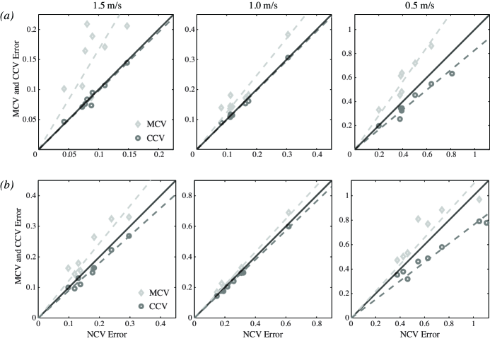
Figure 5: Walking is asymmetric, but neglecting this by training a model on the combined data can nevertheless improve fitting. (a) Step-to-step maps. At all speeds, the mean mirrored cross validation errors (light grey diamonds) were significantly worse than for normal cross validation, indicating that steps were indeed asymmetric. Despite this left–right asymmetry, the mean combined cross validation errors were not significantly different than for normal cross validation at the two fasted walking speeds tested, and, more surprisingly, were actually lower at the slowest walking speed. The slopes of the fitted lines (dashed) determine the relative increase ($m>1$) or decrease ($m<1$) in CV error relative to the NCV error. (b) Stride-to-stride maps. By the same statistical measure, strides were also asymmetric at all speeds, but less substantially so. Moreover, the mean CCV error was lower than mean NCV error at all speeds.

Figure 5(a) compares MCV and CCV errors to NCV error from step-to-step data. MCV errors are (statistically) significantly higher than NCV errors at all speeds ($p_{1.5m/s}=0.004$, $p_{1m/s}=0.008$ and $p_{0.5m/s}=0.004$; one-sided Wilcoxon rank-sign test). This shows that our dataset is indeed dynamically asymmetric between $L\mapsto R$ and $R\mapsto L$.

The comparison of CCV and NCV errors illuminates a different perspective (Figure 5(a)). For speeds of $1.5$ m/s and $1.0$ m/s, CCV and NCV errors were statistically indistinguishable ($p_{1.5m/s}=0.38$ and $p_{1m/s}=0.84$; Wilcoxon rank-sign test), suggesting that for these speeds, the predictive power of a model that assumes symmetry is just as great as one that embraces the asymmetry. More surprisingly, the average CCV error for the slowest speed tested was (statistically) significantly lower than the average NCV error ($p_{0.5m/s}=0.0039$. Wilcoxon one-sided rank-sign test) for the slowest speed ($0.5m/s$). In other words, assuming symmetry (CCV) produces a single step-to-step model that has greater predictive power than is achieved by refining the analysis to produce separate $\{L\mapsto R\}$ and $\{R\mapsto L\}$ step maps.

IV-A2 Stride Maps

We analyzed the dynamical symmetry and the statistical consequences of symmetric modeling on the stride-to-stride transitions. Similar to before, we analyzed two different $\left(\mathcal{N},\mathcal{M}\right)$ combinations, $\left(\mathcal{N},\mathcal{M}\right)=\left(\{L\mapsto L\},\{R\mapsto R\}\right)$ and $\left(\mathcal{N},\mathcal{M}\right)=\left(\{R\mapsto R\},\{L\mapsto L\}\right)$ (Table I). And again, for each category of cross validation, we averaged the CV errors for both combinations of normal and mirrored data. As in the previous section, we first compared NCV and MCV errors to test if the stride-to-stride dataset is statistically asymmetric. The NCV and CCV errors were also compared to contrast the symmetric and asymmetric modeling approaches.

Figure 5(b) compares the MCV and CCV errors to NCV error for stride-to-stride data. MCV errors were higher (on average) than NCV errors for all speeds, and these differences were statistically significant ($p_{1.5m/s}=0.0391$, $p_{1m/s}=0.0117$ and $p_{0.5m/s}=0.0039$; paired one-sided Wilcoxon rank-sign test). This shows that our dataset is dynamically asymmetric between $L\mapsto L$ and $R\mapsto R$.

However, the comparison of NCV and CCV errors in stride-to-stride dataset is more striking than in the step-to-step case in that CCV errors were statistically significantly lower than the NCV errors at all three speeds ($p_{1.5m/s}=0.004$, $p_{1m/s}=0.012$ and $p_{0.5m/s}=0.004$; paired one-sided Wilcoxon rank-sign test).

IV-A3 Model Uncertainty

Cross-validation errors are powerful metrics for comparing the effectiveness of symmetric and asymmetric modeling approaches. However, if two models have similar CVEs, the next thing to address is how well the data constrain the two models—i.e. how much uncertainty there is in the model parameters [55]. This was particularly important for our step-to-step data because symmetric and asymmetric modeling produced indistinguishable CVEs for $1.5$ and $1.0m/s$ walking. This implies that both modeling approaches are equally powerful from the perspective of CVE. However, the parameters of the fitted section map model may exhibit greater variability for the asymmetric modeling approach since it uses less data for fitting.

In order to measure the uncertainty of the models, we adopted following metric:

$$\Xi=\sum\limits_{i=1}^{d}\sum\limits_{j=1}^{d}\sigma_{ij}^{2}$$ (19)

where $\sigma_{ij}^{2}$ is the sample variance of $a_{ij}$, i.e. element at the $i^{th}$ row and $j^{th}$ column of the section map $A_{\mathcal{F}}$ fit during Monte-Carlo iterations of the extended CV method. Symmetric model uncertainty was computed using the fitted matrix samples of the CCV method. Model uncertainties of the $\{L\mapsto R\}$ and $\{R\mapsto L\}$ (and $\{L\mapsto L\}$ and $\{R\mapsto R\}$) maps were averaged to have a single asymmetric model uncertainty for step maps (and stride maps).

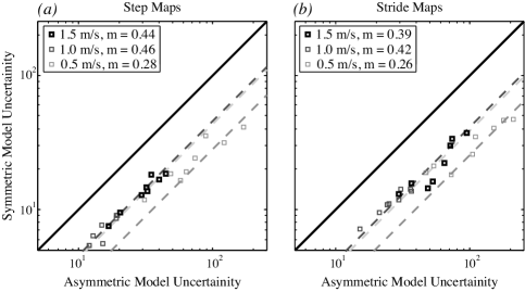
Figure 6: Model uncertainty at all three speeds was lower when symmetry was assumed in both (A) step-to-step and (B) stride-to-stride maps. Each marker compares the model uncertainty with asymmetry and with symmetry of a single individual. Dashed line denotes the best fitted line (passing trough the origin) to the comparison markers. The percentage improvement is given by $(1-m)\times 100$, where $m$ is the slope of the fitted line.

We found that by neglecting asymmetry and fitting a single return map, there was a substantial reduction in model uncertainty for both the step-to-step and stride-to-stride data (Figure 6). Thus, even though in a few cases, the CV errors were similar for NCV and CCV, the models produced using CCV (that is, neglecting asymmetry and pooling the data) are substantially less variable.

For step maps, assuming symmetry substantially lowers model uncertainty; we saw $56\%$, $54\%$, and $72\%$ improvement with symmetric approach for speeds 1.5, 1.0 and 0.5 m/s respectively. All improvements were statistically significant ($p=0.0039$, one-sided Wilcoxon signed-rank test). We observed the same trend with stride maps: $61\%$, $58\%$, and $74\%$ improvement with symmetric approach for speeds 1.5, 1.0 and 0.5 m/s respectively ($p=0.0039$, one-sided Wilcoxon signed-rank test). These results are illustrated in Figure 6.

IV-B Step Return Maps vs. Stride Return Maps

One of the advantages of assuming dynamical bilateral symmetry (i.e. neglecting asymmetry) is that one step becomes the fundamental period of the system; the mapping from step to step defines the return map of the dynamics. On the contrary, if we embrace the asymmetry, the stride becomes the fundamental period. The disadvantage of using stride-to-stride return maps compared to step-to-step maps is a potential loss of signal-to-noise ratio due to the fact that stride maps reduce the temporal resolution. Thus, one can expect that stride-to-stride return maps would have lower predictive power in the CV setting.

In order to compare the predictive powers of step and stride return maps, we analyzed the CVEs by assuming symmetry and fitting lumped return maps to both step and stride data. Specifically, we compared the CCV errors of step and stride data in our method. In order to estimate CCV error of step/stride return map, we took the mean of CCV errors of $\{L\mapsto R\}$ and $\{R\mapsto L\}$/$\{L\mapsto L\}$ and $\{R\mapsto R\}$.

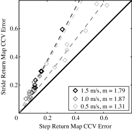
Figure 7: Illustration of the CCV errors of step return maps and stride return maps. Each marker compares the CCV errors of step and stride return maps of a single individual. Dashed lines illustrate the best fitted lines (passing trough the origin) to the comparison markers with $m$ being the associated slope of the line.

The results illustrated in Figure 7 show that there is a dramatic signal-to-noise ratio loss with stride-to-stride return maps and that step-to-step return maps have more predictive power in the CV setting. CCV errors of stride return maps are significantly higher than the ones with step return maps: $79\%$, $87\%$, and $31\%$ more CV error with stride return maps for speeds 1.5, 1.0, and 0.5 m/s respectively. The differences are statistically significant ($p=0.0039$, one-sided Wilcoxon signed-rank test).

V DISCUSSION

In this paper, we focused our attention on bilateral dynamic asymmetry in human walking. Specifically, we introduced a statistical framework based on applying cross validation techniques and fitting linear maps to the data associated with the heel strike events. Our statistical methods allowed us to examine the “wrongness” and “usefulness” of neglecting bilateral dynamic asymmetry.

We applied our methods to data obtained from eight different individuals walking at three different speeds. Based on the results obtained with this data set, we observed that dynamical asymmetry in walking is significant and statistically distinguishable. These results underscore what several studies have previously observed on steady-state parameters [60, 13, 11, 24, 12, 23, 8, 27].

Despite the existence of significant asymmetry, we show that ignoring this and modeling human walking dynamics as symmetric produces significantly more consistent models (Figure 6). Moreover, the predictive power of these symmetric models is higher than (or at worst equal to) their asymmetric counterparts (Figure 5). This shows that neglecting bilateral asymmetry—an inescapable characteristic of the human form—not only provides modeling convenience but, more importantly, produces better models in terms of consistency and predictive power. It is not only “OK” to neglect asymmetry; in some cases, it is better.

One should also note that the slight differences between two “symmetrically” placed sensors (e.g. load cells) can generate an appearance of asymmetry that is not related to the actual system. These asymmetries can affect both limit-cycle symmetry as well as introduce dynamical asymmetries. Fortunately, despite possible measurement asymmetries that would likely exacerbate asymmetries in modeling, a symmetric dynamic model was still preferable for our data. Another limitation to the present study is that participants held their arms crossed while they walked on a treadmill, both of which can affect gait [61, 62]. As instrumentation improves, the questions addressed in this paper can be revisited in unconstrained and/or overground walking and it would be interesting if walking were to be either more or less symmetric in those cases.

Even though we applied our methods to human walking data, they are directly applicable to a wide range of rhythmic dynamical systems in biology and robotics. Specifically, we are interested in behaviors that exhibit alternating (out of phase) gait patterns but are symmetric via reversing the left–right axis for half the stride. This class includes bipedal walking, running, and sprinting [63, 64]; quadrupedal walking, trotting, and pacing [59, 65]; hexapedal alternating tripod gait [66, 67]; and even swimming [68, 69].

In the context of robotics, our methods can be used for diagnostics and calibration since symmetry is considered a desirable property in the design and development of robotic systems. Asymmetric robotic gaits can potentially increase energy expenditure, reduce performance, and introduce a steering bias, hindering the control and operation of the robot. It may be possible to eliminate this steering bias by using existing gait adaptation methods [70, 71] which, to date, requires external instrumentation and specialized arenas. However, our method relies on only internal kinematic measurements which are directly available in most robotic systems, and so perhaps the methods presented in this paper can be used to develop fast and effective calibration methods for field robotics.

On the biological side, there is scientific value in investigating dynamical symmetry across species. Models of biological locomotion can be decomposed into two components: the mechanics of the locomotion (plant), and the neural feedback (controller) [72]. A “less wrong” model of the plant provides better understanding of the controller, and vice-versa [73, 74]. The locomotor pattern of a behaving animal is the closed-loop interaction of the plant and controller. Investigating dynamical symmetry (or asymmetry) in the locomotor gait as well as symmetry (or asymmetry) of the kinematics allows us to better predict the structure of the corresponding neural controller.

With regard to human health in particular, our tools may be useful for understanding motor deficits during locomotion. Specifically, these methods provide an important extension to those that center on kinematic symmetry and its relations to human physiology [10, 4]. Individuals with damage to the musculoskeletal system or nervous system often use asymmetric kinematic walking patterns (e.g. amputees, stroke patients). The kinematic asymmetry can be in the amount of time standing on one leg versus the other, the extent of limb movements, or some combination. An understanding of the underlying dynamical asymmetry (or even symmetry) in these cases would provide more information about the nature of the deficit, and perhaps suggest new targets for focusing rehabilitation treatments.

Finally, an interesting extension of our methods would be analyzing dynamical asymmetry in gaits with categorically asymmetric steady-state kinematics, such as quadrupedal galloping and bounding. The steady-state limit-cycles of such gaits are obviously asymmetric, but the dynamics around those limit-cycles may be symmetric (enough).

VI Data accessibility

The data and codes used for drafting this paper will be able to be accessed via DOI:10.7281/T15Q4T12 (URL: dx.doi.org/10.7281/T15Q4T12). The data used in this paper are the from the baseline walking portion in previous work by Long et al. [75].

VII Authors’ Contributions

MMA developed the statistical tools, analyzed and interpreted the data, and drafted/revised the manuscript. SF, MSM, and NJC interpreted the data, and drafted/revised the manuscript. AL designed and performed the experiments, and revised the manuscript. AJB designed the experiments, interpreted the data, and revised the manuscript.

VIII Acknowledgments and Funding Statement

This material is based upon work supported by the National Science Foundation (NSF) under grants 0845749 and 1230493 to N. J. Cowan and by the National Institutes of Health (NIH) under grant R01-HD048741 to A. J. Bastian. We also thank the reviewers for their insightful comments and suggestions.

Tables

TABLE I: Catalog of normal, $\mathcal{N}$, and associated mirrored, $\mathcal{M}$, datasets combinations used in our CV analysis.

	$\mathcal{N}$	$\mathcal{M}$
Step	$\begin{aligned} \{L\mapsto R\}\\ \{R\mapsto L\}\end{aligned}$	$\begin{aligned} \{R\mapsto L\}\\ \{L\mapsto R\}\end{aligned}$
Stride	$\begin{aligned} \{L\mapsto L\}\\ \{R\mapsto R\}\end{aligned}$	$\begin{aligned} \{R\mapsto R\}\\ \{L\mapsto L\}\end{aligned}$

Figures

References

- [1] Finnerty, J. R., Pang, K., Burton, P., Paulson, D. & Martindale, M. Q., 2004 Origins of bilateral symmetry: Hox and dpp expression in a sea anemone. Science 304, 1335–1337. (doi:10.1126/science.1091946).
- [2] Sadeghi, H., Allard, P., Prince, F. & Labelle, H., 2000 Symmetry and limb dominance in able-bodied gait: a review. Gait Posture 12, 34–45. ISSN 09666362. (doi:10.1016/S0966-6362(00)00070-9).
- [3] Hsiao-Wecksler, E. T., Polk, J. D., Rosengren, K. S., Sosnoff, J. J. & Hong, S., 2010 A review of new analytic techniques for quantifying symmetry in locomotion. Symmetry 2, 1135–1155. (doi:10.3390/sym2021135).
- [4] Finley, J. M., Bastian, A. J. & Gottschall, J. S., 2013 Learning to be economical: the energy cost of walking tracks motor adaptation. J Physiol 591, 1081–1095. (doi:10.1113/jphysiol.2012.245506).
- [5] Lai, K.-A., Lin, C.-J., Jou, I., Su, F.-C. et al., 2001 Gait analysis after total hip arthroplasty with leg-length equalization in women with unilateral congenital complete dislocation of the hip–comparison with untreated patients. J Orthop Res 19, 1147–1152.
- [6] Mattes, S. J., Martin, P. E. & Royer, T. D., 2000 Walking symmetry and energy cost in persons with unilateral transtibial amputations: matching prosthetic and intact limb inertial properties. Arch Phys Med Rehabil 81, 561–568. (doi:10.1016/S0003-9993(00)90035-2).
- [7] Hannah, R., Morrison, J. & Chapman, A., 1984 Kinematic symmetry of the lower limbs. Arch Phys Med Rehabil 65, 155–158.
- [8] Forczek, W. & Staszkiewicz, R., 2012 An evaluation of symmetry in the lower limb joints during the able-bodied gait of women and men. J Hum Kinet 35, 47–57. ISSN 1640-5544. (doi:10.2478/v10078-012-0078-5).
- [9] Karamanidis, K., Arampatzis, A. & Bruggemann, G. P., 2003 Symmetry and reproducibility of kinematic parameters during various running techniques. Med Sci Sports Exerc 35, 1009–1016. (doi:10.1249/01.MSS.0000069337.49567.F0).
- [10] Reisman, D. S., Wityk, R., Silver, K. & Bastian, A. J., 2007 Locomotor adaptation on a split-belt treadmill can improve walking symmetry post-stroke. Brain 130, 1861–1872. (doi:10.1093/brain/awm035).
- [11] Stefanyshyn, D. J. & Engsberg, J. R., 1994 Right to left differences in the ankle joint complex range of motion. Med Sci Sports Exerc 26, 551–555.
- [12] Gundersen, L. A., Valle, D. R., Barr, A. E., Danoff, J. V., Stanhope, S. J. & Snyder-Mackler, L., 1989 Bilateral analysis of the knee and ankle during gait: an examination of the relationship between lateral dominance and symmetry. Phys Ther 69, 640–50. ISSN 0031-9023.
- [13] Law, H., 1987 Microcomputer-based low-cost method for measurement of spatial and temporal parameters of gait. J Biomed Eng 9, 115–120.
- [14] Chodera, J. & Levell, R., 1973 Footprint patterns during walking, pp. 81–90. Perspectives in Biomedical Engineering. Baltimore: University Park Press.
- [15] Chodera, J., 1974 Analysis of gait from footprints. Physiotherapy 60, 179.
- [16] Hamill, J., Bates, B. & Knutzen, K., 1984 Ground reaction force symmetry during walking and running. Res Q Exerc Sport 55, 289–293.
- [17] Menard, M. R., McBride, M. E., Sanderson, D. J. & Murray, D. D., 1992 Comparative biomechanical analysis of energy-storing prosthetic feet. Arch Phys Med Rehabil 73, 451–58.
- [18] Van der Straaten, J. & Scholton, P., 1978 Symmetry and periodicity in gait patterns of normal and hemiplegic children. In Biomechanics VI: proceedings of the Sixth International Congress of Biomechanics, Copenhagen, Denmark, volume 1, p. 287. University Park Press.
- [19] Herzog, W., Nigg, B. M., Read, L. J. & Olsson, E., 1989 Asymmetries in ground reaction force patterns in normal human gait. Med Sci Sports Exerc 21, 110–4. ISSN 0195-9131.
- [20] Carlsöö, S., Dahlöf, A. & Holm, J., 1973 Kinetic analysis of the gait in patients with hemiparesis and in patients with intermittent claudication. Scand J Rehabil Med 6, 166–179.
- [21] Arsenault, A., Winter, D. & Marteniuk, R., 1986 Is there a ‘normal’ profile of emg activity in gait? Med Biol Eng Comput 24, 337–343.
- [22] Marks, M. & Hirschberg, G. G., 1958 Analysis of the hemiplegic gait. Ann NY Acad Sci 74, 59–77.
- [23] Õunpuu, S. & Winter, D. A., 1989 Bilateral electromyographical analysis of the lower limbs during walking in normal adults. Electroencephalogr Clin Neurophysiol 72, 429–438.
- [24] Damholt, V. & Termansen, N., 1978 Asymmetry of plantar flexion strength in the foot. Acta Orthop 49, 215–219.
- [25] Balakrishan, S. & Thornton-Trump, A., 1982 Integral parameters in human locomotion. In Proceeding of the Second Biannual Conference of the Canadian Society for Biomechanics, Human Locomotion II, pp. 12–3.
- [26] Vaughan, C. L., 1996 Are joint torques the Holy Grail of human gait analysis? Hum Movement Sci 15, 423–443.
- [27] Lathrop-Lambach, R. L., Asay, J. L., Jamison, S. T., Pan, X., Schmitt, L. C., Blazek, K., Siston, R. a., Andriacchi, T. P. & Chaudhari, A. M. W., 2014 Evidence for joint moment asymmetry in healthy populations during gait. Gait Posture 40, 526–31. ISSN 1879-2219. (doi:10.1016/j.gaitpost.2014.06.010).
- [28] Crowe, A., Schiereck, P., De Boer, R. & Keessen, W., 1995 Characterization of human gait by means of body center of mass oscillations derived from ground reaction forces. IEEE Trans Biomed Eng 42, 293–303.
- [29] Crowe, A., Schiereck, P., de Boer, R. & Keessen, W., 1993 Characterization of gait of young adult females by means of body centre of mass oscillations derived from ground reaction forces. Gait Posture 1, 61–68.
- [30] Giakas, G. & Baltzopoulos, V., 1997 Time and frequency domain analysis of ground reaction forces during walking: an investigation of variability and symmetry. Gait Posture 5, 189–197. (doi:10.1016/S0966-6362(96)01083-1).
- [31] Box, G. E. P. & Draper, N. R., 1987 Empirical Model-Building and Response Surfaces. Wiley.
- [32] Altendorfer, R., Koditschek, D. E. & Holmes, P., 2004 Stability analysis of legged locomotion models by symmetry-factored return maps. Int J Robot Res 23, 979–999. (doi:10.1177/0278364904047389).
- [33] Chevallereau, C., Grizzle, J. W. & Shih, C.-L., 2009 Asymptotically stable walking of a five-link underactuated 3-d bipedal robot. IEEE Trans Robot 25, 37–50. (doi:10.1109/TRO.2008.2010366).
- [34] Ankarali, M. M. & Saranli, U., 2010 Stride-to-stride energy regulation for robust self-stability of a torque-actuated dissipative spring-mass hopper. Chaos 20. (doi:10.1063/1.3486803).
- [35] De, A. & Koditschek, D. E., 2015 The penn jerboa: A platform for exploring parallel composition of templates. arXiv preprint arXiv:1502.05347 .
- [36] Hurmuzlu, Y. & Basdogan, C., 1994 On the measurement of dynamic stability of human locomotion. Trans ASME 116, 30–36.
- [37] Seyfarth, A., Geyer, H. & Herr, H., 2003 Swing-leg retraction: a simple control model for stable running. J Exp Biol 206, 2547–2555. (doi:10.1242/jeb.00463).
- [38] Holmes, P. J., Full, R. J., Koditschek, D. E. & Guckenheimer, J., 2006 The dynamics of legged locomotion: Models, analyses, and challenges. SIAM Rev 48, 207–304. (doi:10.1137/S0036144504445133).
- [39] Revzen, S. & Guckenheimer, J. M., 2011 Finding the dimension of slow dynamics in a rhythmic system. J R Soc Interface 9, 957–971. (doi:10.1098/rsif.2011.0431).
- [40] Ankarali, M. M., Şen, H. T., De, A., Okamura, A. M. & Cowan, N. J., 2014 Haptic feedback enhances rhythmic motor control by reducing variability, not improving convergence rate. J Neurophysiol 111, 1286–1299. (doi:10.1152/jn.00140.2013).
- [41] Guckenheimer, J. & Holmes, P., 1991 Nonlinear Oscillations, Dynamical Systems, and Bifurcations of Vector Fields. Springer.
- [42] Muir, G. D. & Whishaw, I. Q., 1999 Complete locomotor recovery following corticospinal tract lesions: measurement of ground reaction forces during overground locomotion in rats. Behav Brain Res 103, 45–53. (doi:10.1016/S0166-4328(99)00018-2).
- [43] Pourcelot, P., Audigie, F., Degueurce, C., Denoix, J. & Geiger, D., 1997 Kinematic symmetry index: a method for quantifying the horse locomotion symmetry using kinematic data. Vet Res 28, 525.
- [44] Miller, R. H., Meardon, S. A., Derrick, T. R. & Gillette, J. C., 2008 Continuous relative phase variability during an exhaustive run in runners with a history of iliotibial band syndrome. J Appl Biomech 24, 262–270.
- [45] Kurz, M. J., Arpin, D. J. & Corr, B., 2012 Differences in the dynamic gait stability of children with cerebral palsy and typically developing children. Gait Posture 36, 600–604.
- [46] Donelan, J. M., Kram, R. & Kuo, A. D., 2002 Mechanical work for step-to-step transitions is a major determinant of the metabolic cost of human walking. J Exp Biol 205, 3717–3727.
- [47] Ankarali, M. & Saranli, U., 2011 Control of underactuated planar pronking through an embedded spring-mass hopper template. Auton Robot 30, 217–231. ISSN 0929-5593. (doi:10.1007/s10514-010-9216-x).
- [48] Saranli, U., Arslan, O., Ankarali, M. M. & Morgul, O., 2010 Approximate analytic solutions to non-symmetric stance trajectories of the passive spring-loaded inverted pendulum with damping. Nonlinear Dynam 62, 729–742. (doi:10.1007/s11071-010-9757-8).
- [49] Blickhan, R. & Full, R. J., 1993 Similarity in multilegged locomotion: Bouncing like a monopode. J Comp Physiol A 173, 509–517. (doi:10.1007/BF00197760).
- [50] Westervelt, E., Grizzle, J. & Koditschek, D., 2003 Hybrid zero dynamics of planar biped walkers. IEEE Trans Autom Control 48, 42–56. (doi:10.1109/TAC.2002.806653).
- [51] Duindam, V. & Stramigioli, S., 2009 Modeling and analysis of walking robots. In Modeling and Control for Efficient Bipedal Walking Robots, pp. 93–127. Springer.
- [52] Lee, J., Sponberg, S. N., Loh, O. Y., Lamperski, A. G., Full, R. J. & Cowan, N. J., 2008 Templates and anchors for antenna-based wall following in cockroaches and robots. IEEE Trans Robot 24, 130–143. (doi:10.1109/TRO.2007.913981).
- [53] Ankarali, M. M., 2015 Variability, Symmetry, and Dynamics in Human Rhythmic Motor Control. Ph.D. thesis, Johns Hopkins University.
- [54] Shao, J., 1993 Linear model selection by cross-validation. J Am Statist Assoc 88, 486–494.
- [55] Madhav, M. S., Stamper, S. A., Fortune, E. S. & Cowan, N. J., 2013 Closed-loop stabilization of the jamming avoidance response reveals its locally unstable and globally nonlinear dynamics. J Exp Biol 216, 4272–4284. (doi:10.1242/jeb.088922).
- [56] Rao, C. & Wu, Y., 2005 Linear model selection by cross-validation. J Stat Plan Inference 128, 231–240. (doi:10.1016/j.jspi.2003.10.004).
- [57] Yang, Y., 2007 Consistency of cross validation for comparing regression procedures. Ann Stat pp. 2450–2473.
- [58] Arlot, S. & Celisse, A., 2010 A survey of cross-validation procedures for model selection. Stat Surv 4, 40–79.
- [59] Collins, J. J. & Stewart, I. N., 1993 Coupled nonlinear oscillators and the symmetries of animal gaits. J Nonlinear Sci 3, 349–392. (doi:10.1007/BF02429870).
- [60] Allard, P., Lachance, R., Aissaoui, R. & Duhaime, M., 1996 Simultaneous bilateral 3-d able-bodied gait. Hum Movement Sci 15, 327–346.
- [61] Ortega, J. D., Fehlman, L. A. & Farley, C. T., 2008 Effects of aging and arm swing on the metabolic cost of stability in human walking. J Biomech 41, 3303–3308.
- [62] Dingwell, J., Cusumano, J., Cavanagh, P. & Sternad, D., 2001 Local dynamic stability versus kinematic variability of continuous overground and treadmill walking. J Biomech Eng 123, 27–32.
- [63] Mann, R. A. & Hagy, J., 1980 Biomechanics of walking, running, and sprinting. Am J Sports Med 8, 345–350. (doi:10.1177/036354658000800510).
- [64] Collins, S., Ruina, A., Tedrake, R. & Wisse, M., 2005 Efficient bipedal robots based on passive-dynamic walkers. Science 307, 1082–5. (doi:10.1126/science.1107799).
- [65] Buehler, M., Battaglia, R., Cocosco, A., Hawker, G., Sarkis, J. & Yamazaki, K., 1998 Scout: A simple quadruped that walks, climbs, and runs. In Proc IEEE Int Conf Robot Autom, volume 2, pp. 1707–1712. IEEE.
- [66] Full, R. J. & Tu, M. S., 1990 Mechanics of six-legged runners. J Exp Biol 148, 129–146.
- [67] Saranli, U., Buehler, M. & Koditschek, D. E., 2001 RHex: A simple and highly mobile hexapod robot. Int J Robot Res 20, 616–631. (doi:10.1177/02783640122067570).
- [68] Sfakiotakis, M., Lane, D. M. & Davies, J. B. C., 1999 Review of fish swimming modes for aquatic locomotion. IEEE J Ocean Eng 24, 237–252. (doi:10.1109/48.757275).
- [69] Ijspeert, A. J., Crespi, A., Ryczko, D. & Cabelguen, J.-M., 2007 From swimming to walking with a salamander robot driven by a spinal cord model. Science 315, 1416–1420. (doi:10.1126/science.1138353).
- [70] Weingarten, J., Lopes, G. A. D., Buehler, M., Groff, R. E. & Koditschek, D., 2004 Automated gait adaptation for legged robots. In Proc IEEE Int Conf Robot Autom, volume 3, pp. 2153–2158. (doi:10.1109/ROBOT.2004.1307381).
- [71] Galloway, K., Clark, J., Yim, M. & Koditschek, D., 2011 Experimental investigations into the role of passive variable compliant legs for dynamic robotic locomotion. In Proc IEEE Int Conf Robot Autom, pp. 1243–1249. (doi:10.1109/ICRA.2011.5979941).
- [72] Roth, E., Sponberg, S. & Cowan, N. J., 2014 A comparative approach to closed-loop computation. Curr Opin Neurobiol 25, 54–62. (doi:10.1016/j.conb.2013.11.005).
- [73] Cowan, N. J. & Fortune, E. S., 2007 The critical role of locomotion mechanics in decoding sensory systems. J Neurosci 27, 1123–1128. (doi:10.1523/JNEUROSCI.4198-06.2007).
- [74] Cowan, N. J., Ankarali, M. M., Dyhr, J. P., Madhav, M. S., Roth, E., Sefati, S., Sponberg, S., Stamper, S. A., Fortune, E. S. & Daniel, T. L., 2014 Feedback control as a framework for understanding tradeoffs in biology. Integr Comp Biol 54, 223–237. ISSN 1540-7063. (doi:10.1093/icb/icu050).
- [75] Long, A. W., Finley, J. M. & Bastian, A. J., 2015 A Marching-Walking Hybrid Induces Step Length Adaptation and Transfers to Natural Walking. J Physiol. ISSN 0022-3077. (doi:10.1152/jn.00779.2014).