Structure of chromomagnetic fields in the glasma

Abstract

The initial stage of a heavy ion collision is dominated by nonperturbatively strong chromoelectric and -magnetic fields. The spatial Wilson loop provides a gauge invariant observable to probe the dynamics of the longitudinal chromomagnetic field. We discuss recent results from a real time lattice calculation of the area-dependence of the expectation value of the spatial Wilson loop. We show that at relatively early times after the collision, a universal scaling as a function of the area emerges at large distances for very different initial conditions, with a nontrivial critical exponent. A similar behavior has earlier been seen in calculations of the gluon transverse momentum spectrum, which becomes independent of the initial spectrum of gauge fields. We also show the distribution of eigenvalues of the spatial Wilson loop and the fluctuations of its real and imaginary parts.

Nuclear Physics A T. Lappi et al. nupha Nuclear Physics A

1 Introduction

The initial stages of a heavy ion collision are dominated by nonperturbatively strong gluonic fields. These fields are characterized by a momentum and length scale generated by nonlinear gluonic interactions, the saturation scale $Q_{\mathrm{s}}$. In the “Color Glass Condensate” (CGC) effective theory description of QCD, the initial “glasma”[1] chromomagnetic and -electric fields are predominantly longitudinal [1, 2, *Fries:2006pv]. Because of the large ($\sim 1/\alpha_{\mathrm{s}}$) occupation numbers of the gluonic states the glasma fields are essentially classical, and obey the Yang-Mills equations of motion. From these equations their time dependence can be solved either analytically in an expansion in the field strength [4, *Blaizot:2008yb] or numerically on a lattice [6, *Krasnitz:2001qu, *Krasnitz:2003jw, *Lappi:2003bi, 10]. Most earlier numerical studies have concentrated on the gluon spectrum, obtained from Coulomb gauge-fixed field correlators. It would, however, be interesting to have an independent, manifestly gauge invariant way to study the dynamics of the softer field modes $k_{T}\lesssim Q_{\mathrm{s}}$. One possibility for such an observable, first studied in this context in Ref. [11], is the spatial Wilson loop. We will here discuss results from a more recent calculation [12] that extends this work in many ways, with ${N_{\mathrm{c}}}=3$ colors (instead of ${N_{\mathrm{c}}}=2$ in [11]), measurements over a larger range of areas and most importantly a more systematical comparison of different initial conditions for the equations of motion, provided by different CGC parametrizations of the two colliding nuclei. We stress that this work concerns the detailed structure of the boost invariant background fields and does not include their unstable quantum fluctuations that eventually lead to an isotropization of the system [13, *Gelis:2013rba].

2 Classical Yang-Mills

Before the collision the individual fields of projectile and target are two dimensional pure gauges; in light cone gauge,

$$\alpha^{i}_{m}({\mathbf{x}_{T}})=\frac{i}{g}\,V_{m}({\mathbf{x}_{T}})\,\partial^{i}V_{m}^{\dagger}({\mathbf{x}_{T}})$$ (1)

where $m=1,\,2$ labels the projectile and target, respectively. Here $V_{m}$ are light-like SU(${N_{\mathrm{c}}}$) Wilson lines that describe the propagation of a lightlike probe through the color field; thus they can be related to e.g. the DIS cross section. In the CGC they are stochastic variables drawn from some probability distribution. We have in this calculation compared results from three well-motivated possibilities for this probability distribution. The first one is the MV model [15, *McLerran:1994ka, *McLerran:1994vd], where the Wilson lines are obtained from a classical color charge density $\rho$ as

$$V({\mathbf{x}_{T}})=\mathbb{P}\exp\left\{i\int\,\mathrm{d}x^{-}g^{2}\frac{1}{\boldsymbol{\nabla}_{T}^{2}}\rho^{a}({\mathbf{x}_{T}},x^{-})\right\},$$ (2)

where $\mathbb{P}$ denotes path-ordering in $x^{-}$. In the MV model the densities $\rho$ are assumed to have a local Gaussian distribution parametrized by a single dimensionful paramater $\mu$, related to the saturation scale as $Q_{\mathrm{s}}\sim g^{2}\mu$. The numerical implementation of the MV model in this context is described in detail in Ref. [10].

At higher collision energies one needs to resum large corrections of order $\alpha_{\mathrm{s}}\ln s$ from additional gluon bremsstrahlung. In the CGC framework this is achieved by the JIMWLK renormalization group equation, which describes the dependence of the probability distribution of the Wilson lines on $y\equiv\ln\sqrt{s}$. The two other probability distributions studied in this work result from solving the JIMWLK equation with either fixed or running QCD coupling, with the MV model as an initial condition. For details on the numerical procedure used to do this we refer the reader to Refs. [18, *Rummukainen:2003ns, *Lappi:2012vw].

3 Results

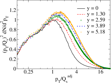
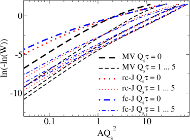
Figure 1: Left: Gluon spectrum in the glasma in the symmetric (midrapidity) case, expressed in terms of the scaling variable $p_{T}/Q_{\mathrm{s}}$. The initial condition at $y=0$ corresponds to the MV model, while after $y=\ln\sqrt{s}\approx 6$ units of JIMWLK evolution (here at fixed coupling) the spectrum in the ultraviolet is different. Figure from Ref. [21], with an error in the vertical axis labeling corrected. Right: Area dependence of the Wilson loop expectation value. The thick lines are the initial condition and thinner ones correspond to later times. Three different initial conditions are shown, corresponding to the MV model and fixed and running coupling JIMWLK evolution, labeled “fc-J” and “rc-J” respectively.

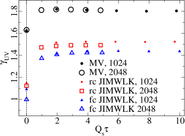
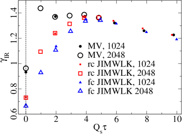
Figure 2: The scaling exponents $\gamma$ for small area (left) and large area (right) Wilson loops, as a function of time $\tau$. Comparison between MV, fixed and running coupling JIMWLK initial conditions and different lattice sizes.

Let us start by a reminder of earlier results for the gluon spectrum [21], shown in Fig.1 (left). What was observed was the following: in the dilute $p_{T}\gtrsim Q_{\mathrm{s}}$ regime where final state interactions are relatively weak, the spectrum depends on the initial conditions, being harder with the JIMWLK distribution than the MV one, in agreement with expectations from $k_{T}$-factorization. In the infrared part $p_{T}\lesssim Q_{\mathrm{s}}$, on the other hand, there is a remarkable universality, both in the shape and the normalization, with $\,\mathrm{d}N/\,\mathrm{d}^{2}p_{T}\sim 1/p_{T}$ independently of the initial condition.

We then turn to the results for the spatial Wilson loop, which is defined as the trace of a path ordered exponential of the gauge field around a closed path of area $A$ in the transverse plane:

$$W(A)=\frac{1}{{N_{\mathrm{c}}}}\left<\,\mathrm{Tr}\,\mathbb{P}\exp\left\{ig\oint_{\partial A}\,\mathrm{d}{\mathbf{x}_{T}}\cdot\mathbf{A}_{T}\right\}\right>.$$ (3)

In Ref. [12] we have found that the dependence of $W$ on the area $A$ of the loop is well described by the functional form

$$W(A)=\exp\left\{-(\sigma A)^{\gamma}\right\},$$ (4)

with separate parameters $\sigma$ and $\gamma$ in the large (“IR”) and small (“UV”) area regimes:

$$\mathrm{IR:} e^{0.5}<AQ_{\mathrm{s}}^{2}<e^{5}$$ (5)

$$\mathrm{UV:} e^{-3.5}<AQ_{\mathrm{s}}^{2}<e^{-0.5}~{}.$$ (6)

Figure 1 (right) shows the result for the Wilson loop expectation value, for different initial conditions and different times $\tau$. For small area Wilson loops the behavior parallels that of the gluonspectrum at high $p_{T}$: the differences in the initial condition manifest themselves in the area dependence, both at the initial time $\tau=0$ and later. For large loops, the area dependence for different initial conditions is also different at $\tau=0$. After a time $\tau\sim 3/Q_{\mathrm{s}}$, however, the simulations with different initial conditions collapse onto a universal curve with both the slope $\gamma$ and the normalization $\sigma$ independent of the initial condition. Interestingly, instead of the area law $\gamma=1$ that one might expect, the universal behavior is characterized by a nontrivial exponent $\gamma\approx 1.2$. The time dependence of the scaling exponents is shown in Fig. 2.

4 Fluctuations of the Wilson lines

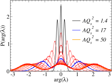
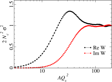
Figure 3: Left: Probability distribution of the phase angle of the Wilson line eigenvalues $\lambda$, for different loop areas. Right: variance of the real and imaginary part of the trace of the Wilson loop, as a function of the area of the loop. Simulations with running coupling JIMWLK initial conditions, at $Q_{\mathrm{s}}\tau=5$.

As a further study beyond what was reported in Ref. [12] we have recently looked at the statistical properties of the Wilson line distribution in more detail. Figure 3 (left) shows the probability distribution of the eigenvalues of the Wilson lines $\lambda=e^{i\varphi}$. One sees a progression from a three-peaked structure around $\varphi=0$ for small areas (close to $W(A)=1$) to a distribution that is close to the expectation

$$P(\varphi)=\frac{1}{2\pi}\left(1+\frac{2}{3}\cos(3\varphi)\right)$$ (7)

from a completely random ensemble of SU(3) matrices for large areas. Figure 3 (right) shows the variance of the real and imaginary parts of the trace of the Wilson loop. These start from a very small value for small areas, where the SU(3) matrix is constrained to be very close to the identity, and approach the random SU(3) matrix expectation for the variance

$$\sigma^{2}=\frac{1}{2{N_{\mathrm{c}}}^{2}}$$ (8)

for large areas.

References

- [1] T. Lappi and L. McLerran, Nucl. Phys. A772, 200 (2006), [arXiv:hep-ph/0602189]
- [2] D. Kharzeev, A. Krasnitz and R. Venugopalan, Phys. Lett. B545, 298 (2002), [arXiv:hep-ph/0109253]
- [3] R. J. Fries, J. I. Kapusta and Y. Li, arXiv:nucl-th/0604054
- [4] A. Kovner, L. D. McLerran and H. Weigert, Phys. Rev. D52, 6231 (1995), [arXiv:hep-ph/9502289]
- [5] J.-P. Blaizot and Y. Mehtar-Tani, Nucl. Phys. A818, 97 (2009), [arXiv:0806.1422 [hep-ph]]
- [6] A. Krasnitz and R. Venugopalan, Nucl. Phys. B557, 237 (1999), [arXiv:hep-ph/9809433]
- [7] A. Krasnitz, Y. Nara and R. Venugopalan, Phys. Rev. Lett. 87, 192302 (2001), [arXiv:hep-ph/0108092]
- [8] A. Krasnitz, Y. Nara and R. Venugopalan, Nucl. Phys. A727, 427 (2003), [arXiv:hep-ph/0305112]
- [9] T. Lappi, Phys. Rev. C67, 054903 (2003), [arXiv:hep-ph/0303076]
- [10] T. Lappi, Eur. Phys. J. C55, 285 (2008), [arXiv:0711.3039 [hep-ph]]
- [11] A. Dumitru, Y. Nara and E. Petreska, Phys. Rev. D88, 054016 (2013), [arXiv:1302.2064 [hep-ph]]
- [12] A. Dumitru, T. Lappi and Y. Nara, Phys. Lett. B734, 7 (2014), [arXiv:1401.4124 [hep-ph]]
- [13] J. Berges, K. Boguslavski, S. Schlichting and R. Venugopalan, Phys. Rev. D89, 074011 (2014), [arXiv:1303.5650 [hep-ph]]
- [14] T. Epelbaum and F. Gelis, Phys. Rev. Lett. 111, 232301 (2013), [arXiv:1307.2214 [hep-ph]]
- [15] L. D. McLerran and R. Venugopalan, Phys. Rev. D49, 2233 (1994), [arXiv:hep-ph/9309289]
- [16] L. D. McLerran and R. Venugopalan, Phys. Rev. D49, 3352 (1994), [arXiv:hep-ph/9311205]
- [17] L. D. McLerran and R. Venugopalan, Phys. Rev. D50, 2225 (1994), [arXiv:hep-ph/9402335]
- [18] J.-P. Blaizot, E. Iancu and H. Weigert, Nucl. Phys. A713, 441 (2003), [arXiv:hep-ph/0206279 [hep-ph]]
- [19] K. Rummukainen and H. Weigert, Nucl. Phys. A739, 183 (2004), [arXiv:hep-ph/0309306 [hep-ph]]
- [20] T. Lappi and H. Mäntysaari, Eur. Phys. J. C73, 2307 (2013), [arXiv:1212.4825 [hep-ph]]
- [21] T. Lappi, Phys. Lett. B703, 325 (2011), [arXiv:1105.5511 [hep-ph]]