Nuclear deformation at finite temperature

Abstract

Deformation, a key concept in our understanding of heavy nuclei, is based on a mean-field description that breaks the rotational invariance of the nuclear many-body Hamiltonian. We present a method to analyze nuclear deformations at finite temperature in a framework that preserves rotational invariance. The auxiliary-field Monte-Carlo method is used to generate the statistical ensemble and calculate the probability distribution associated with the quadrupole operator. Applying the technique to nuclei in the rare-earth region, we identify model-independent signatures of deformation and find that deformation effects persist to higher temperatures than the spherical-to-deformed shape phase-transition temperature of mean-field theory.

Motivation.— Mean-field theory is a useful method for studying correlated many-body systems. However, it often breaks symmetries, making it difficult to compare its results with physical spectra that preserve these symmetries. In addition, although mean-field theory often predicts sharp phase transitions at finite temperature, they are washed out in finite-size systems. The challenge is to find tools to study the properties of finite-size systems within a framework that preserves the underlying symmetries while also allowing calculation of the quantities that describe symmetry breaking in mean-field theory.

In nuclear physics, this issue is especially important in the understanding of heavy deformed nuclei, which are of wide experimental and theoretical interest. The current theory of these nuclei is based on self-consistent mean-field (SCMF) theory, which predicts both spherical and deformed ground states su3 depending on the nucleus. SCMF is a convenient tool to study their intrinsic structure but it breaks rotational invariance, a prominent symmetry in nuclear spectroscopy. The occurrence of large deformations in the ground state and at low excitations gives rise to rotational bands and large electric quadrupole transition intensities between states within the bands. At higher excitations, much less is known experimentally. Characterization of this part of the spectrum is needed for accurate calculation of the nuclear level density, which is very sensitive to deformation and other structure effects; observed level densities in rare-earth nuclei at the neutron evaporation threshold vary by more than an order of magnitude RIPL . In addition, nuclear fission is a phenomenon of shape dynamics, and calculation of fission rates for excited nuclei requires their level densities as a function of deformation pe09 .

Here we investigate nuclear deformation at finite temperature using the auxilliary-field Monte Carlo (AFMC) method, which is well suited to the study of the evolution of nuclear properties with excitation energy while preserving rotational invariance. In particular, we calculate the distribution of the quadrupole operator in the lab frame and demonstrate that it exhibits model-independent signatures of deformation. We use moments of this distribution to calculate rotationally invariant observables, which allow us to extract effective values of the intrinsic deformation and its fluctuations. Deformations have been studied previously by the AFMC method, but with an ad hoc prescription to extract the intrinsic-frame properties al96 . The methods presented here should be applicable to other finite-size systems in which correlations beyond the mean field are important.

Methodology.— Formally, we can examine the statistical characteristics of nuclei at finite excitations by calculating the thermal expectation values of observables $\hat{O}$ associated with the property of interest, $\langle{\hat{O}}\rangle={{\rm Tr}\,({\hat{O}}e^{-\beta\hat{H}})/{\rm Tr}\,e^{-\beta\hat{H}}}$. Here $\beta^{-1}$ is the temperature and $\hat{H}$ is the Hamiltonian, which we assume to be rotationally invariant. We denote operators in the many-particle space with a circumflex, to be distinguished from operators in the single-particle space, which are ordinary matrices, denoted by bold-face symbols. Also, we denote the trace over the full many-particle Fock space as ${\rm Tr}$ and the trace of matrices in the single-particle space by ${\rm tr}$. The probability distribution of an operator $\hat{O}$, $P_{\beta}(o)={{{\rm Tr}(\delta[{\hat{O}}-o)e^{-\beta\hat{H}}]}/{\rm Tr}e^{-\beta\hat{H}}}$ can be calculated using the Fourier representation of the $\delta$ function:

$$P_{\beta}(o)={1\over{\rm Tr}\,e^{-\beta\hat{H}}}\int_{-\infty}^{\infty}{d\varphi\over 2\pi}e^{-i\varphi o}\,{\rm Tr}\,\left(e^{i\varphi\hat{O}}e^{-\beta\hat{H}}\right).$$ (1)

Eq. (1) is well-known for one-body observables $\hat{O}$ that commute with the Hamiltonian, e.g., the number operator and the $z$-component of the angular momentum al07 .

Nuclear shape is different in that the relevant operators, e.g., the quadrupole operators, do not commute with the Hamiltonian. Nevertheless, it is possible with Eq. (1) to define the distribution of quantum-mechanical observables that carry information about deformation as well as energy. The distribution (1) can be expressed in terms of the many-particle eigenstates of $\hat{O}$ and $\hat{H}$ as

$$P_{\beta}(o)=\sum_{n}\delta(o-o_{n})\sum_{m}\langle o,n|e,m\rangle^{2}e^{-\beta e_{m}}.$$ (2)

Here $|o,n\rangle$ are eigenstates of $\hat{O}$ satisfying ${\hat{O}}|o,n\rangle=o_{n}|o,n\rangle$ and similarly for $|e,m\rangle$. Eq. (2) is valid whether or not the operators $\hat{O}$ and $\hat{H}$ commute. When they do commute, they share a common basis of eigenstates such that $\langle o,n|e,m\rangle=\delta_{m,n}$ and the distribution (2) reduces to its more familiar form $P_{\beta}(o)=\sum_{n}\delta(o-o_{n})e^{-\beta e_{n}}$. Note that in a finite model space the eigenvalues $o_{n}$ form a discrete set and $P_{\beta}(o)$ is a finite sum of $\delta$ functions.

In this work we consider the observable $\hat{O}$ to be the spectroscopic mass quadrupole operator $\hat{Q}_{20}=\sum_{i}\left(2z_{i}^{2}-x_{i}^{2}-y_{i}^{2}\right)$ where the sum is taken over all nucleons. The probability distribution $P_{\beta}(q)$ of $\hat{Q}_{20}$ is defined as in Eq. (1) with $\hat{O}=\hat{Q}_{20}$ and $o=q$.

As we will show, this distribution can be accurately computed by the AFMC method. However, the intrinsic-frame properties are not directly accessed by the operator $\hat{Q}_{20}$, which is a laboratory-frame observable. We shall demonstrate in this work that nevertheless the distribution $P_{\beta}(q)$ is sensitive to deformation effects and that the main properties of the deformation in the intrinsic frame can be recovered from moments of this distribution.

Intrinsic frame quantities may be defined in terms of the expectation values of rotationally invariant combinations of the quadrupole tensor operator $\hat{Q}_{2\mu}$ ($\mu=-2,\ldots,2$) ku72 ; cl86 . The lowest-order invariant is quadratic, $\hat{Q}\cdot\hat{Q}=\sum_{\mu}(-)^{\mu}\hat{Q}_{2\mu}\hat{Q}_{2-\mu}$. There is one third-order invariant defined by coupling three quadrupole operators to angular momentum zero, $(\hat{Q}\times\hat{Q})\cdot\hat{Q}=\sqrt{5}\sum_{\mu_{1},\mu_{2},\mu_{3}}\left(\begin{array}[]{ccc}2&2&2\\ \mu_{1}&\mu_{2}&\mu_{3}\end{array}\right)\hat{Q}_{2\mu_{1}}\hat{Q}_{2\mu_{2}}\hat{Q}_{2\mu_{3}}$. The fourth- and fifth-order invariants are also unique Q-commutation and we define them as $(\hat{Q}\cdot\hat{Q})^{2}$ and $(\hat{Q}\cdot\hat{Q})((\hat{Q}\times\hat{Q})\cdot\hat{Q})$, respectively. When the invariant is unique at a given order, its expectation value can be computed directly from the lab-frame moments of $\hat{Q}_{20}$, defined by $\langle\hat{Q}_{20}^{n}\rangle_{\beta}=\int q^{n}P_{\beta}(q)dq$. The conversion factors are given in Table I.

n	2	3	4	5
invariant	5	$-5(7/2)^{1/2}$	35/3	$-(11/2)(7/2)^{1/2}$
rotor	1/5	2/35	3/35	4/77

Table 1: First line: the ratio of the expectation value of the invariant of order $n$ (see text) to the $n$-th moment of $\hat{Q}_{20}$. Second line: the $n$-th moment of $\hat{Q}_{20}$ for the rigid rotor in units of $q_{0}^{n}$ ($q_{0}$ is the rotor’s intrinsic quadrupole moment).

AFMC.— We shall use the AFMC to evaluate the distribution in Eq. (1) for $\hat{O}=\hat{Q}_{20}$. AFMC is arguably the most powerful computational tool for finding the ground states and thermal properties in large-dimension many-particle spaces. It is based on the Hubbard-Stratonovich representation HS of the imaginary-time propagator, $e^{-\beta\hat{H}}=\int D[\sigma]G_{\sigma}\hat{U}_{\sigma}$, where $D[\sigma]$ is the integration measure, $G(\sigma)$ is a Gaussian weight, and $\hat{U}_{\sigma}$ is a one-body propagator of non-interacting nucleons moving in auxiliary fields $\sigma$. Practical implementations require that the Hamiltonian be restricted to one- and two-body terms, and that the two-body terms have the so-called good sign sign . The method has been applied to nuclei in the framework of the configuration-interaction shell model la93 ; al94 ; SMMC , where it is called the shell-model Monte Carlo (SMMC). It has been particularly successful in calculating statistical properties of nuclei such as level densities LD . The distribution of $\hat{Q}_{20}$ is obtained from the Monte Carlo sampling of fields $\sigma$ as a ratio of averages

$$P_{\beta}(q)=\left\langle\frac{{\rm Tr}\left[\delta(\hat{Q}_{20}-q)\hat{U}_{\sigma}\right]}{{\rm Tr}{\hat{U}}_{\sigma}}\Phi_{\sigma}\right\rangle_{W}\langle\Phi_{\sigma}\rangle_{W}^{-1}\;,$$ (3)

Here $\langle X\rangle_{W}=\int D[\sigma]W_{\sigma}X_{\sigma}/\int D[\sigma]W_{\sigma}$, where $W_{\sigma}=G_{\sigma}|{\rm Tr}\,\hat{U}_{\sigma}|$ is used for the Monte Carlo sampling and $\Phi_{\sigma}={\rm Tr}\,\hat{U}_{\sigma}/|{\rm Tr}\,\hat{U}_{\sigma}|$ is the Monte Carlo sign function.

For a given $\hat{U}_{\sigma}$, we carry out the $\hat{Q}_{20}$ projection using a discretized version of the Fourier decomposition in Eq. (1). We take an interval $[-q_{\rm max},q_{\rm max}]$ and divide it into $2M+1$ equal intervals of length $\Delta q=2q_{\rm max}/(2M+1)$. We define $q_{m}=m\Delta q$, where $m=-M,\ldots,M$, and approximate the quadrupole-projected trace in (3) by

$${\rm Tr}\left(\delta(\hat{Q}_{20}-q_{m})U_{\sigma}\right)\!\!\approx\!\!{1\over 2q_{\rm max}}\!\!\sum_{k=-M}^{M}\!\!\!e^{-i\varphi_{k}q_{m}}{\rm Tr}(e^{i\varphi_{k}\hat{Q}_{20}}\hat{U}_{\sigma})\;,$$ (4)

where $\varphi_{k}=\pi k/q_{\rm max}$ ($k=-M,\ldots,M$). Since $\hat{Q}_{20}$ is a one-body operator and $\hat{U}_{\sigma}$ is a one-body propagator, the Fock space many-particle traces on the r.h.s. of Eq. (4) reduce to determinants in the single-particle space ${\rm Tr}\left(e^{i\varphi_{k}\hat{Q}_{20}}\hat{U}_{\sigma}\right)=\det\left(1+e^{i\varphi_{k}{\bf Q}_{20}}{\bf U}_{\sigma}\right)$. Here ${\bf Q}_{20}$ and ${\bf U}_{\sigma}$ are the matrices representing, respectively, $\hat{Q}_{20}$ and $\hat{U}_{\sigma}$, in the single-particle space. In practice, projections are carried on the neutron and proton number operators as well to fix the $Z$ and $N$ of the ensemble SMMC .

We found the thermalization of $\hat{Q}_{20}^{n}$ to be slow with the pure Metropolis sampling. This can be overcome by augmenting the Metropolis-generated configurations by rotating them through a properly chosen set of $N_{\Omega}$ rotation angles $\Omega$. In practice, it is easier to rotate the observables, i.e., we replace $\langle e^{i\varphi\hat{Q}_{20}}\rangle_{\sigma}$ by ${1\over N_{\Omega}}\sum_{j}\langle e^{i\varphi\hat{Q}_{20}(\Omega_{j})}\rangle_{\sigma}$. Here $\hat{Q}_{20}(\Omega)=\hat{R}\hat{Q}_{20}\hat{R}^{-1}$ with $\hat{R}$ being the rotation operator for angle $\Omega$. Details will be given elsewhere.

We next discuss a few simple examples that can be treated analytically or nearly so.

Rigid rotor.— As a first simple example, we consider an axially symmetric rigid rotor with an intrinsic quadrupole moment $q_{0}$ in its ground state. The distribution of its spectroscopic quadrupole operator in the laboratory frame $Q_{20}=q_{0}(3\cos^{2}\theta-1)/2$ can be calculated in closed form. For a prolate rotor ($q_{0}>0$)

$$P_{\rm g.s.}(q)=\left\{\begin{array}[]{cc}\left(\sqrt{3}q_{0}\sqrt{1+2{q\over q_{0}}}\right)&\mbox{for $-{q_{0}\over 2}\leq q\leq q_{0}$}\\ 0&\mbox{otherwise}\end{array}\right.\;.$$ (7)

This distribution is shown in Fig. 1. The oblate rotor ($q_{0}<0$) distribution is obtained from (7) by replacing $q$ with $-q$ and $q_{0}$ with $|q_{0}|$.

Figure 1: The ground-state distribution $P_{\rm g.s.}(q)$ vs $q/q_{0}$ for a prolate rotor with intrinsic quadrupole moment $q_{0}$.

The moments of the distribution (7) can be calculated from a simple recursion relation; their values for $2\leq n\leq 5$ are given in Table I.

²⁰Ne.— As a simple illustration in nuclear spectroscopy, we consider the light deformed nucleus ²⁰Ne. The orbital part of the single-particle wave functions are taken to be the states of the $N=2$ harmonic oscillator shell, i.e., the $sd$-shell. The single-particle eigenvalues of ${\bf Q}_{20}$ are -2, 1, and 4 (in units of $b^{2}$ b ) with degeneracies of 6, 4 and 2, respectively. The many-particle eigenvalues of $\hat{Q}_{20}$ for ²⁰Ne in the valence $sd$-shell thus range from $-8$ to $16$ with a uniform spacing of $3$. The distribution $P_{\beta}(q)$ at $\beta=0$ is just the distribution of these eigenvalues.

We have used this nucleus as a simple test of the AFMC. Here we take the single-particle energies according to the USD interaction brown and consider an attractive quadrupole-quadrupole interaction $-\chi\tilde{Q}\cdot\tilde{Q}$, with $\tilde{Q}_{2\mu}=\sum_{i}r_{i}^{2}Y_{2\mu}(\hat{r}_{i})$ and $\chi={8\pi\over 5}{38.5\over A^{5/3}}$ MeV$/b^{4}$ la89 . In Fig. 2 we show the quadrupole distribution of the ²⁰Ne ground state. The discrete nature of the many-particle eigenvalues of $\hat{Q}_{20}$ is evident; the distribution is a set $\delta$ functions at integers $-8,-5,\ldots,13,16$. The envelope of the strengths has the skewed shape that looks qualitatively similar to the prolate rigid-rotor distribution.

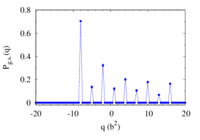
Figure 2: The AFMC ground-state quadrupole distribution $P_{\rm g.s.}(q)$ for ²⁰Ne. The sharp $\delta$-like peaks demonstrate the discrete nature of the spectrum of $\hat{Q}_{20}$ and their envelope resembles the prolate rigid-rotor distribution in Fig. 1.

SCMF.— It is instructive to compare our results with those of the thermal SCMF, e.g., the finite-temperature Hartree-Fock-Bogoliubov (HFB) approximation. The HFB solution is characterized by temperature-dependent one-body density matrix $\bm{\rho}_{\beta}$ and pairing tensor $\bm{\kappa}_{\beta}$. In general, two types of phase transitions can occur vs temperature, a pairing transition and a deformed-to-spherical shape transition go86 ; ag00 ; ma03 . A shape phase transition is also the generic result of a Landau theory in which the order parameter is the quadrupole deformation tensor al86 . The vast majority of deformed HFB ground states are axially symmetric de10 , i.e., $\langle\hat{Q}_{2\mu}\rangle=0$ for $\mu\neq 0$. The second-order invariant $\langle\hat{Q}\cdot\hat{Q}\rangle$ may be calculated in HFB by using Wick’s theorem

$$\langle\hat{Q}\cdot\hat{Q}\rangle=Q_{0}^{2}+\sum_{\mu}(-)^{\mu}{\rm tr}\left[{\bf Q}_{2\mu}\,({\bf 1}-\bm{\rho}_{\beta})\,{\bf Q}_{2-\mu}\,\bm{\rho}_{\beta}\right]$$

$$+\sum_{\mu}(-)^{\mu}{\rm tr}\left[{\bf Q}_{2\mu}\,\bm{\kappa}_{\beta}\,{\bf Q}^{T}_{2-\mu}\,\bm{\kappa}_{\beta}^{\ast}\right]\;,$$ (8)

where $Q_{0}\equiv{\rm tr}({\bf Q}_{20}\bm{\rho}_{\beta})$ is the intrinsic axial quadrupole moment. The remaining terms on the r.h.s. of (Nuclear deformation at finite temperature) represent the contributions due to quantal and thermal fluctuations. We shall compare our AFMC results for rare-earth nuclei with the HFB theory in the next section.

Rare-earth nuclei.— Here we present results for rare-earth nuclei. The single-particle orbitals are taken from a Woods-Saxon potential plus spin-orbit interaction; they span the $50-82$ shell plus $1f_{7/2}$ orbital for protons and the $82-126$ shell plus $0h_{11/2},1g_{9/2}$ orbitals for neutrons. We use the same interaction as in Refs. al08 ; oz13 . The quadrupole moments are scaled by a factor of 2 to account for the model space truncation.

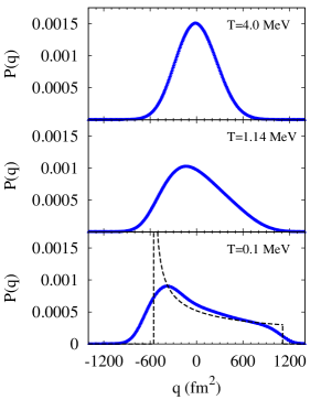
Figure 3: Probability distributions $P_{\beta}(q)$ for ¹⁵⁴Sm at $T=0.1$ MeV, $T=1.14$ MeV (shape transition temperature) and $T=4$ MeV. The low-temperature distribution is compared with the rigid-rotor distribution (dashed line) and reflects the strongly deformed character of this nucleus.

We first examine ¹⁵⁴Sm, a strongly deformed nucleus with an intrinsic quadrupole moment of $Q_{0}\sim 1600$ fm², as determined experimentally from in-band electric quadrupole transitions ra01 . AFMC $P_{\beta}(q)$ distributions are shown in Fig. 3 at three temperatures. The distributions appear continuous because the many-particle eigenvalues of $\hat{Q}_{20}$ are closely spaced. At the lowest temperature of $T=0.1$ MeV (bottom panel), $e^{-\beta\hat{H}}$ effectively projects out the ground-state band. We observe the characteristic skewed distribution of the prolate rotor. The dashed line is the rotor distribution (7) with $q_{0}$ taken at the HFB value of $Q_{0}$. The middle panel is the distribution at the HFB shape transition temperature, $T=1.14$ MeV. The distribution is less skewed, but nevertheless it retains some trace of a prolate character. The HFB excitation energy at this temperature is about 25 MeV, much higher than energies of interest for spectroscopy and for the neutron-capture reaction. The top panel shows the distribution at $T=4$ MeV. At this high excitation the distribution is featureless and close to a Gaussian.

We have also calculated $P_{\beta}(q)$ for ¹⁴⁸Sm, which is spherical in its HFB ground state. They are more symmetric and change less with temperature, consistent with the absence of a coherent quadrupole moment.

Invariants.— Fig. 4 shows the second-order invariant $\langle\hat{Q}\cdot\hat{Q}\rangle$ vs temperature $T$ for ¹⁴⁸Sm and ¹⁵⁴Sm. The AFMC results (circles) are compared with the HFB results (dashed lines) of Eq. (Nuclear deformation at finite temperature). In HFB, $\langle\hat{Q}\cdot\hat{Q}\rangle$ for ¹⁴⁸Sm can be entirely attributed to the fluctuation terms in (Nuclear deformation at finite temperature). There is a small kink at $T=0.4$ MeV associated with the pairing transition, but by and large the curve is flat. The same is true of the AFMC curve. In contrast, $\langle\hat{Q}\cdot\hat{Q}\rangle$ in ¹⁵⁴Sm is very different at low temperatures. In HFB, the intrinsic quadrupole moment $Q_{0}$ is large, and it persists up to a temperature of the order of $1$ MeV, close to the spherical-to-deformed phase-transition temperature. The AFMC results are in semiquantitative agreement at the lowest temperatures showing that the coherent intrinsic quadrupole moment is not an artifact of the HFB. The sharp kink characterizing the HFB shape transition go86 ; ma03 is washed out, as is expected in a finite-size system. Nevertheless a signature of this phase transition remains in the rapid decrease of $\langle Q\cdot Q\rangle$ with temperature. In AFMC deformation effects survive well above the transition temperature, in that $\langle Q\cdot Q\rangle$ continues to be enhanced beyond its uncorrelated mean-field value.

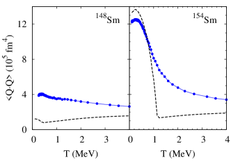
Figure 4: $\langle Q\cdot Q\rangle$ vs temperature $T$ for the spherical ¹⁴⁸Sm (left) and the deformed ¹⁵⁴Sm (right). The AFMC results (solid circles) are compared with the HFB results (dashed lines).

The second- and third-order invariants can be used to define effective values of the intrinsic shape parameters $\beta,\gamma$ beta of the collective Bohr model (BM, , Sec. 6B-1a). The model assumes an intrinsic frame in which the quadrupole deformation parameters $\alpha_{2\mu}=\sqrt{5\pi}\langle\hat{Q}_{2\mu}\rangle/3r_{0}^{2}A^{5/3}$ are expressed as $\alpha_{20}=\beta\cos\gamma$, $\alpha_{22}=\alpha_{2-2}=\frac{1}{\sqrt{2}}\beta\sin\gamma$, and $\alpha_{2\pm 1}=0$. Effective $\beta$ and $\gamma$ can then be determined from the corresponding invariants

$$\beta=\frac{\sqrt{5\pi}}{3r_{0}^{2}A^{5/3}}\langle\hat{Q}\cdot\hat{Q}\rangle^{1/2}\;;\;\;\cos 3\gamma=-\sqrt{7\over 2}{\langle(\hat{Q}\times\hat{Q})\cdot\hat{Q}\rangle\over\langle\hat{Q}\cdot\hat{Q}\rangle^{3/2}}\;.$$ (9)

In addition, we can extract a measure $\Delta\beta$ of the fluctuations in $\beta$ using the second- and fourth-order invariants

$$\left({\Delta\beta/\beta}\right)^{2}={\left[\langle(\hat{Q}\cdot\hat{Q})^{2}\rangle-\langle\hat{Q}\cdot\hat{Q}\rangle^{2}\right]^{1/2}/\langle\hat{Q}\cdot\hat{Q}\rangle}\;.$$ (10)

The invariants themselves are calculated from the moments of $P_{\beta}(q)$ using the relations in Table I. As expected, the deformed ¹⁵⁴Sm has a larger deformation $\beta$ than ¹⁴⁸Sm ($0.232$ vs $0.137$), but a smaller deformation angle $\gamma$ ($13.4^{\circ}$ vs $21.6^{\circ}$) that is closer to an axial shape. The deformed nucleus is more rigid in that it has a smaller $\Delta\beta/\beta$, $0.51$ for ¹⁵⁴Sm vs $0.72$ for ¹⁴⁸Sm.

Summary.— We have demonstrated that the distribution of the axial quadrupole operator can be computed in the AFMC method, and that it conveys important information about deformation and the intrinsic shapes of nuclei at finite temperature. In particular, the expectation values of $\beta^{2}$, $\beta^{3}\cos 3\gamma$ and the fluctuation in $\beta^{2}$ can be extracted as a function of temperature. With these moments, it should be possible to construct models of the joint level density distribution $\rho(\beta,E_{x})=\rho(E_{x})P_{E_{x}}(\beta)$, where $\rho(E_{x})$ is the total level density and $P_{E_{x}}(\beta)$ is the intrinsic shape distribution at excitation energy $E_{x}$. This joint distribution is an important component in the theory of fission and will be discussed in a future publication.

Acknowledgments.— Y. Alhassid acknowledges the hospitality of the Institute of Nuclear Theory in Seattle, where part of this work was completed. We thank H. Nakada for the HFB code. This work was supported in part by the U.S. DOE grant Nos. DE-FG02-91ER40608 and DE-FG02-00ER411132. Computational cycles were provided by the NERSC high performance computing facility and by the facilities of the Yale University Faculty of Arts and Sciences High Performance Computing Center.

References

- (1) The representation provides an alternate way to study deformation effects va02 , but it has not been widely applied to heavy nuclei.
- (2) C.E. Vargas, J.G. Hirsch, and J.P. Draayer, Nucl. Phys. A 697, 655 (2002).
- (3) The RIPL3 database containing tables of experimental level densities can be accessed at https://www-nds.iaea.org/RIPL-3/resonances/.
- (4) J.C. Pei, W. Nazarewicz, J.A. Sheikh, and A.K. Kerman, Phys. Rev. Lett. 102, 192501 (2009).
- (5) Y. Alhassid, G.F. Bertsch, D.J. Dean, and S.E. Koonin, Phys. Rev. Lett. 77, 1444 (1996).
- (6) Y. Alhassid, S. Liu, and H. Nakada, Phys. Rev. Lett. 99, 162504 (2007).
- (7) K. Kumar, Phys. Rev. Lett. 28, 249 (1972).
- (8) D. Cline, Ann. Rev. Nucl. Part. Sci. 36, 683 (1986).
- (9) Strictly speaking the uniqueness of the fourth- and fifth-order invariants holds when the operators commute among themselves. The quadrupole operators commute in coordinate space but generally not in a truncated shell model space. However, the effects due to their non-commutation is small.
- (10) J. Hubbard, Phys. Rev. Lett. 3, 77 (1959); R. L. Stratonovich, Dokl. Akad. Nauk SSSR [Sov. Phys. - Dokl.] 115, 1097 (1957).
- (11) Small bad-sign interaction terms can be treated using the extrapolation method of Ref. al94 .
- (12) Y. Alhassid, D.J. Dean, S.E. Koonin, G. Lang, and W.E. Ormand, Phys. Rev. Lett. 72, 613 (1994).
- (13) G.H. Lang, C.W. Johnson, S.E. Koonin, and W.E. Ormand, Phys. Rev. C 48, 1518 (1993).
- (14) S.E. Koonin, D.J. Dean, and K. Langanke, Phys. Rep. 278, 2 (1997); Y. Alhassid, Int. J. Mod. Phys. B 15, 1447 (2001).
- (15) H. Nakada and Y. Alhassid, Phys. Rev. Lett. 79, 2939 (1997); Y. Alhassid, S. Liu, and H. Nakada, Phys. Rev. Lett. 83, 4265 (1999).
- (16) The oscillator length parameter is defined to give a ground-state wave function of the form .
- (17) B.A. Brown and W.A. Richter, Phys. Rev. C 74, 034315 (2006).
- (18) B. Lauritzen and G.F. Bertsch, Phys. Rev. C 39, 2412 (1989).
- (19) A.L. Goodman, Phys. Rev. C 33, 2212 (1986).
- (20) V. Martin, J. L. Egido and L. M. Robledo, Phys. Rev. C 68, 034327 (2003).
- (21) B. K. Agrawal, T. Sil, J. N. De, and S. K. Samaddar, Phys. Rev. C 62, 044307 (2000).
- (22) Y. Alhassid, S. Levit, and J. Zingman, Phys. Rev. Lett. 57, 539 (1986).
- (23) J.-P. Delaroche, et al., Phys. Rev. C 81, 014303 (2010).
- (24) Y. Alhassid, L. Fang and H. Nakada, Phys. Rev. Lett. 101, 082501 (2008).
- (25) C. Özen, Y. Alhassid, and H. Nakada, Phys. Rev. Lett. 110, 042502 (2013).
- (26) S. Raman, C.W. Nestor, and P. Tikkanen, At. Data Nucl. Data Tables 78, 1 (2001).
- (27) We use the symbol for both the inverse temperature and the dimensionless deformation parameter; the meaning should be clear from the context.
- (28) A. Bohr and B. Mottelson, Nuclear Structure, Vol. II (Benjamin, 1975).