Gene-level pharmacogenetic analysis on survival outcomes using gene-trait similarity regression

Abstract

Gene/pathway-based methods are drawing significant attention due to their usefulness in detecting rare and common variants that affect disease susceptibility. The biological mechanism of drug responses indicates that a gene-based analysis has even greater potential in pharmacogenetics. Motivated by a study from the Vitamin Intervention for Stroke Prevention (VISP) trial, we develop a gene-trait similarity regression for survival analysis to assess the effect of a gene or pathway on time-to-event outcomes. The similarity regression has a general framework that covers a range of survival models, such as the proportional hazards model and the proportional odds model. The inference procedure developed under the proportional hazards model is robust against model misspecification. We derive the equivalence between the similarity survival regression and a random effects model, which further unifies the current variance component-based methods. We demonstrate the effectiveness of the proposed method through simulation studies. In addition, we apply the method to the VISP trial data to identify the genes that exhibit an association with the risk of a recurrent stroke. The TCN2 gene was found to be associated with the recurrent stroke risk in the low-dose arm. This gene may impact recurrent stroke risk in response to cofactor therapy.

, and

t1Equal contribution. t2Supported by National Institutes of Health Grants R01 MH084022 and P01 CA142538. t3Supported by National Institutes of Health Grants R01 CA140632 and P01 CA142538. t4Supported by National Institutes of Health Grant U01 HG005160.

1 Introduction

Genetic variations play a significant role in drug responses. A gene that participates in a particular physiological mechanism might influence the response to a specific therapeutic agent that targets the mechanism. Identifying these influential genes may help to clarify if an individual might benefit from or be harmed by the therapy. Understanding the genetic diversity of drug responses can help to identify medications that maximize treatment effectiveness and minimize the risk of adverse effects for individuals. Such an understanding will also lead to improved risk stratification, prevention and treatment strategies for human diseases. Pharmacogenetics studies show how an adverse reaction or positive response to pharmaceutical treatment is affected by an individual’s genetic makeup and has the potential to deliver both public health and economic benefits rapidly. With the recent advancements in high-throughput technologies, it is becoming common for pharmacogenetic researches to systematically investigate genetic markers across the genome. Nevertheless, appropriate and efficient analysis of the data remains a challenge.

Gene- or pathway-based analyses can assess pharmacogenetic effects more effectively than single-marker based analyses [Goldstein, Tate and Sisodiya (2003); Goldstein (2005)]. First, there often exist obvious candidate genes and pathways that metabolize the drug and carry variants that are relevant to the drug responses. Responses to therapies usually involve complex relationships between gene variants within the same molecular pathway or functional gene set. When applied to pharmacogenetic studies, gene- or pathway-based methods might identify multiple variants of subtle effects that are missed by single marker-based methods. Second, pharmacogenetic studies typically enroll only a moderate number of patients, which limits the power of the association detection. Gene-based analyses have been shown to yield higher power than standard single marker and haplotype analyses. This type of analysis can particularly facilitate studies on rare-event drug responses, such as adverse reactions, where it could take many years to collect a sufficient number of samples to obtain adequate power for standard analyses. In gene-based analyses, the association signals are aggregated across variants, and the total number of tests is reduced; the amplification of the association signals and the alleviation of the multiple testing burdens result in improved power.

Our study was motivated by the need for a gene-based analysis of the time-to-event data of the Vitamin Intervention for Stroke Prevention (VISP) trial [Toole, Malinow and Chambless (2004); Hsu, Sides and Mychalecky (2011)]. Our goal is to assess the association between the recurrent stroke risk and the 9 candidate genes involved in the homocystein (Hcy) metabolic pathway (see Data section for more details). In our preliminary analysis, we used the Cox proportional hazards (PH) model [Cox (1972)] to perform single-SNP screening on 69 SNPs across 9 genes from 969 individuals. There were no SNPs past the significance threshold after accounting for multiple testing. However, the top 6 hits, thresholding at unadjusted $p$-values $<$0.05, were concentrated in two genes. Specifically, 4 SNPs are from TCN2 (i.e., rs1544468, rs731991, rs2301955 and rs2301957 have Wald’s test $p$-values of 0.0065, 0.0072, 0.0346 and 0.0346, resp.) and 2 SNPs are from CTH (i.e., rs648743 and rs663465 each have a Wald’s test $p$-value of 0.0115). The Kaplan–Meier curves of these 6 SNPs are shown in Figure 1 and indicate the potential for different risk patterns among different variants at these loci. The clustering within the two genes suggests that it would be more efficient to combine the individual signal strengths and model the joint effect of multiple loci in a gene.

Figure 1: The Kaplan–Meier survival curves for the top 6 SNPs identified from the single SNP association analysis with risk of recurrent stroke.

We perform the gene-based analysis using a gene-trait similarity regression inspired by Haseman–Elston regression from linkage analysis [Elston et al. (2000); Haseman and Elston (1972)] and haplotype similarity tests for regional association [Beckmann et al. (2005); Qian and Thomas (2001); Tzeng et al. (2003)]. First, we quantify the genetic and trait similarities for each pair of individuals. The genetic similarity is determined using identity by state (IBS) methods. The trait similarity is obtained from the covariance of the transformed survival time conditional on the covariates. We then regress the trait similarity on the genetic similarity and test the regression coefficient to detect the genetic association. There are several gene-based approaches for censored time-to-event phenotypes in the literature, including Goeman et al. (2005) and Lin and colleagues [Cai, Tonini and Lin (2011); Lin et al. (2011)]. In these approaches, the multimarker effects were modeled under the Cox PH model using linear random effects [Goeman et al. (2005)] or a nonparametric function induced by a kernel machine [Cai, Tonini and Lin (2011); Lin et al. (2011)]. The global effect of a gene was detected by testing for the corresponding genetic variance component. These approaches were found to be superior in identifying pathways or genes that are associated with survival.

For many years, similarity-based methods have been successfully used to evaluate gene-based associations in quantitative and binary traits [Beckmann et al. (2005); Lin and Schaid (2009); Qian and Thomas (2001); Tzeng et al. (2003); Wessel and Schork (2006)]. Our work makes such approaches available for survival phenotypes. In addition, our similarity regression covers a variety of risk models, including the commonly used PH model and the proportional odds (PO) model. Furthermore, we show that the coefficient of the similarity regression obtained for survival phenotypes can be reexpressed as a variance component of a certain working random effects model. Such results facilitate the derivation of the test statistic and unify the similarity model and previous variance component methods [Goeman et al. (2005); Cai, Tonini and Lin (2011); Lin et al. (2011)]. Specifically, under the Cox PH model, our test statistic is equivalent to the test statistic defined by a kernel machine approach [Lin et al. (2011)]. We also show that the test statistic can be robust to model misspecification. Specifically, the proposed test gives the correct type I error even if the true risk model is misspecified. However, the correct specification of the true risk model generally leads to a test with better power. Finally, we demonstrate the utility of the similarity regression by identifying the important TCN2 gene in the VISP study. The significance of TCN2 to stroke risk has been reported by other association studies [Giusti et al. (2010); Low et al. (2011)] and has been supported by molecular biology evidence [Afman et al. (2003); von Castel-Dunwoody et al. (2005)]. Our findings further suggest potential interactions between TCN2 and B12 supplementation. This new information furthers the possibility that TCN2 could be utilized to predict recurrent strokes, identify at-risk individuals and identify therapeutic targets for ischemic stroke.

2 Data

The VISP study was a prospective, double-blind, randomized clinical trial [Toole, Malinow and Chambless (2004)]. The trial was designed to study if high doses of folic acid, vitamin B6 and vitamin B12 reduce the risk of a recurrent stroke as compared to low doses of these vitamins. The trial enrolled patients who were 35 or older, had a nondisabling cerebral infarction within 120 days of randomization, and had Hcy levels in the top quartile of the U.S. population. Subjects were randomly assigned to receive daily doses of either a high-dose formulation (containing 25 mg vitamin B6, 0.4 mg vitamin B12 and 2.5 mg folic acid) or a low-dose formulation (containing 200 $\mu$g vitamin B6, 6 $\mu$g vitamin B12 and 20 $\mu$g folic acid). Patient recruitment began in August 1997 and was completed in December 2001. A total of 3680 participants were enrolled at 56 clinical sites across the United States, Canada and Scotland. The patients were followed for a maximum of two years, and the average follow-up duration was 1.7 years. In the VISP genetic study, 2206 participants provided informed consent and blood samples. The SNP genotypes of 9 genes related to the enzymes and cofactors in the Hcy metabolic pathway were collected: BHMT1, BHMT2, CBS, CTH, MTHFR, MTR, MTRR, TCN1 and TCN2 [Hsu, Sides and Mychalecky (2011)]. In a previous study, Hsu, Sides and Mychalecky (2011) conducted single-SNP analyses on targeted loci (e.g., Hcy-associated variants) to examine the genetic association with the recurrent stroke risk. In the low-dose arm, the authors found that TCN2 SNP rs731991 under a recessive mode was associated with the risk of a recurrent stroke with an unadjusted log-rank test $p$-value of 0.009. The associations for the remaining SNPs within the 9 genes in the low-dose arm were not studied. We extend this previous analysis to all 9 genes using a gene-based approach. After quality control screening of the data (e.g., removing loci with $>$99% missing proportion or Hardy–Weinberg disequilibrium under additive mode and removing individuals with missing genotypes), the analysis included 969 individuals in the low-dose arm with 69 recessively coded SNPs.

3 Gene-trait similarity regression for survival traits

3.1 The model

For individual $i$ $(i=1,2,\ldots,n)$, let $T_{i}$ denote the survival time of interest and $C_{i}$ denote the censoring time. We observe $\tilde{T}_{i}=\min(T_{i},C_{i})$ and the censoring indicator $\delta_{i}=I(T_{i}\leq C_{i})$. In addition, let $X_{i}$ denote the $K\times 1$ vector of covariates and g_mi denote the allele count vector of marker $m$ for person $i$, where the length of g_mi, $\ell_{m}$ is the number of distinct alleles at marker $m$, $m=1,2,\ldots,M$. For example, for a tri-allelic locus $m$, g${}_{mi}=(1,0,1)^{T}$ if person $i$ has genotype “$A_{1}A_{3}$” and $(0,2,0)^{T}$ if person $i$ has genotype “$A_{2}A_{2}$.”

For each pair of individuals $i$ and $j$, we measure the genetic similarity, $S_{ij}$, of the targeted gene and the trait similarity, $Z_{ij}$. The genetic similarity is quantified using the weighted IBS sum across the $M$ markers in the gene, that is, $S_{ij}=\sum_{m=1}^{M}w_{m}S_{ij}^{m}$, where $S_{ij}^{m}=2$ if $|\mbox{{g}}_{m,i}-\mbox{{g}}_{m,j}|$ is a zero vector, $S_{ij}^{m}=1$ if $|\mbox{{g}}_{m,i}-\mbox{{g}}_{m,j}|$ contains exactly two $1$’s (and if $\ell_{m}>2$, the remaining entries are $0$), and $S_{ij}^{m}=0$ otherwise. The weights, $w_{m}$, are specified to up-weight or down-weight a variant based on certain features. Examples include weights that are based on allele frequencies, the degree of evolutionary conservation or the functionality of the variations [Wessel and Schork (2006); Schaid (2010a, 2010b); Price et al. (2010)]. We can use the minor allele frequency of marker $m$, denoted as $q_{m}$, to up-weight similarities that are contributed by rare variants. Specifically, one can set a moderate weight, such as $w_{m}=q_{m}^{-{3}/{4}}$ [Pongpanich, Neely and Tzeng (2012)] or $w_{m}=q_{m}^{-1}$ [Tzeng et al. (2011)], to promote similarity attributed by rare alleles, or use a more extreme weight, such as $w_{m}=(1-q_{m})^{24}$ [Wu et al. (2011)], to target rare variants only.

The trait similarity, $Z_{ij}$, is quantified as follows. First, we define $Y_{i}=H(T_{i})$, where $H(\cdot)$ is an (unspecified) monotonic increasing transformation function, such as the logarithm transformation $Y_{i}=\log(T_{i})$. Assume that the conditional mean of $Y_{i}$ given the covariates and genes is $E(Y_{i}\mid X_{i},{g_{i}})=\theta+X_{i}^{T}\gamma+{g_{i}}$, where $\theta$ is the intercept, $g_{i}$ is the multi-locus genetic effect of person $i$, and $\gamma$ is the $K$-dimensional covariate effect. Further, define $\mu_{i}^{0}=\theta+X_{i}^{T}\gamma$. The trait similarity is defined as the product of the paired residuals adjusting for the covariate effects, that is, $Z_{ij}=(Y_{i}-\mu_{i}^{0})(Y_{j}-\mu_{j}^{0})$. The expected value of the trait similarity is the covariance between the transformed survival times of subjects $i$ and $j$.

The gene-trait similarity regression has the form

$$E(Z_{ij}\mid X_{i},X_{j})=b\times S_{ij},\qquad i\neq j.$$ (1)

Just as in Tzeng et al. (2009, 2011), the regression has a zero intercept and does not have the covariate term $X_{i}X_{j}$ because the baseline and covariate effects have been adjusted when defining $Z_{ij}$. This argument will become more obvious from the viewpoint of variance components in the following subsection. Under model (1), the overall association of a gene can be evaluated by testing the null hypothesis: $b=0$.

3.2 Score test for the gene-level effect

We derive the score test statistic based on the equivalence between the similarity regression and a mixed model. This equivalence is demonstrated as follows. Consider a working mixed model for the transformed survival time:

$$Y_{i}=H(T_{i})=X_{i}^{T}\gamma+{g_{i}}+\theta+\varepsilon_{i},$$ (2)

where ${(g_{1},\ldots,g_{n})}^{T}\sim N$ $(0,\tau S)$ with $S=\{S_{ij}\}_{i,j=1}^{n}$, that is, the covariance between $g_{i}$ and $g_{j}$ depends on the genetic similarity between subjects $i$ and $j$, and $\varepsilon_{i}^{\ast}\equiv\theta+\varepsilon_{i}$, $i=1,\ldots,n$ are independently and identically distributed with a known distribution that is independent of $X_{i}$ and ${g_{i}}$. Given $X_{i}$ and $g_{i}$, model (2) specifies a general class of linear transformation models [Cheng, Wei and Ying (1995)], which contains many popular survival models as special cases. For example, when $\varepsilon_{i}^{\ast}$ follows the standard extreme value distribution, the linear transformation model becomes the PH model [Cox (1972)]. When $\varepsilon_{i}^{\ast}$ follows the standard logistic distribution, the linear transformation model becomes the PO model [Bennett (1983)].

Under (2), the conditional expectation of the trait similarity between individuals $i$ and $j$ ($i\neq j$) is

$$E(Z_{ij}\mid X_{i},X_{j}) = \operatorname{cov}(Y_{i},Y_{j}\mid X_{i},X_{j})=\operatorname{cov}\bigl{(}g_{i}+\varepsilon_{i}^{\ast},g_{j}+\varepsilon_{i}^{\ast}\bigr{)}$$

$$= \operatorname{cov}(g_{i},g_{j})$$

$$= \tau\times S_{ij}.$$

Therefore, we have $b=\tau$, that is, the regression coefficient in the similarity regression (1) is the genetic variance component in the mixed model (2). This motivates us to develop a score test for the variance component in the working model. As shown in the Appendix, the score test statistics for $\tau=0$ can be written as

$$Q_{n}=\frac{1}{n}(\hat{r}_{1},\ldots,\hat{r}_{n})S(\hat{r}_{1},\ldots,\hat{r}_{n})^{T},$$

where

$$\hat{r}_{i} = \int_{0}^{\infty}\hat{\omega}_{i}(t)\,dM_{i}(t;\hat{\gamma},\hat{H})$$

$$= \delta_{i}\frac{\dot{\lambda}\{\hat{H}(\tilde{T}_{i})-\hat{\gamma}^{T}X_{i}\}}{\lambda\{\hat{H}(\tilde{T}_{i})-\hat{\gamma}^{T}X_{i}\}}-\lambda\bigl{\{}\hat{H}(\tilde{T}_{i})-\hat{\gamma}^{T}X_{i}\bigr{\}},$$

$$M_{i}(t;\gamma,H) = \delta_{i}I(\tilde{T}_{i}\leq t)-\int_{0}^{t}I(\tilde{T}_{i}\geq s)\,d\Lambda\bigl{\{}H(s)-\gamma^{T}X_{i}\bigr{\}},$$

$\hat{\omega}_{i}(t)=\dot{\lambda}\{\hat{H}(t)-\hat{\gamma}^{T}X_{i}\}/\lambda\{\hat{H}(t)-\hat{\gamma}^{T}X_{i}\}$, and $S$ is as defined after equation (2). Here, $\lambda(\cdot)$ and $\Lambda(\cdot)$ are the hazard and cumulative hazard functions of $\varepsilon_{i}^{\ast}$, respectively, $\dot{\lambda}(\cdot)$ is the first derivative of $\lambda(\cdot)$, and $\hat{\gamma}$ and $\hat{H}(\cdot)$ are the estimates of $\gamma$ and $H(\cdot)$, respectively, in model (2) under the null hypothesis: $\tau=0$. For example, if the PH model is imposed, that is, $\lambda(u)=\dot{\lambda}(u)=e^{u}$, the estimators $\hat{\gamma}$ and $\hat{\Gamma}(\cdot)\equiv e^{\hat{H}(\cdot)}$ can be taken as the maximum partial likelihood estimator and Breslow’s estimator, respectively. Under this case, $\hat{\omega}_{i}(t)\equiv 1$ and $\hat{r}_{i}=\delta_{i}-\hat{\Gamma}(\tilde{T}_{i})\exp(-\hat{\gamma}^{T}X_{i})$, that is, the martingale residual for the null model. If the PO model is used, that is, $\lambda(u)=e^{u}/(1+e^{u})$ and $\dot{\lambda}(u)=e^{u}/(1+e^{u})^{2}$, we have $\hat{\omega}_{i}(t)=1/[1+\exp\{\hat{H}(t)-\hat{\gamma}^{T}X_{i}\}]$. In general, $\gamma$ and $H(\cdot)$ can be estimated using the martingale-based estimating equations [Chen, Jing and Ying (2002)] or the nonparametric maximum likelihood estimation method [Zeng and Lin (2006)] for the semiparametric linear transformation model. In the Appendix, we show that under the null hypothesis the test statistic, $Q_{n}$, asymptotically follows a weighted $\chi^{2}$ distribution where the weights can be estimated consistently. The $p$-values can then be calculated numerically using a resampling method or moment-matching approximations [Pearson (1959); Duchesne and Lafaye De Micheaux (2010)].

We note that the proposed score test can be robust to the misspecification of the true survival model. As an illustration, consider the test derived under the PH model. Based on the results for the robust inference of the PH model [Lin and Wei (1989)], when the PH model is misspecified, the maximum partial likelihood estimator, $\hat{\gamma}$, and Breslow’s estimator, $\hat{\Gamma}(\cdot)$, do not converge to the true parameters but converge to some deterministic values $\gamma^{\ast}$ and $\Gamma^{\ast}(\cdot)$ under certain regularity conditions. The corresponding $r_{i}^{\ast}=\delta_{i}-\Gamma^{\ast}(\tilde{T}_{i})\exp(-X_{i}^{T}\gamma^{\ast})$ is not a martingale residual but has a mean of 0 under the null hypothesis. Therefore, it can be shown that $Q_{n}$ converges in distribution to a weighted $\chi^{2}$ distribution under the null hypothesis even with model misspecification. As shown in our simulation studies, the proposed score test derived under the PH model still gives correct type-I error when the true model is the PO model. However, the power of the test depends on the assumed working model. In general, the test derived under the true risk model may have better power.

4 Results of the analysis of the VISP trial data

We now return to the VISP trial to evaluate the association between the recurrent stroke risk and the 9 candidate genes studied in Hsu, Sides and Mychalecky (2011). In our analysis, we conducted a gene-based screening on the 9 genes using the low-dose samples. After removing loci with $>$1% of missingness and subjects with missing genotypes, there were 969 individuals with 69 polymorphic SNPs under recessive coding. Of the 969 individuals, 86 experienced a recurrent stroke (i.e., 91.1% censoring). We used the proposed similarity regression (referred to as SimReg) with inverse allele frequency weights $w_{m}=q_{m}^{-{3}/{4}}$, that is, the weight recommended in Pongpanich, Neely and Tzeng (2012) when analyzing a mixture of common and rare variants. We calculated the $p$-values of the SimReg statistics using the resampling method. Specifically, we computed the nonzero eigenvalues, $\hat{\xi}_{1},\ldots,\hat{\xi}_{d}$, of $\hat{\Sigma}$ as defined in the Appendix. We generated $10^{4}$ sets of $(\chi_{1,1}^{2},\ldots,\chi_{1,d}^{2})$. Each set consisted of $d$ independently and identically distributed $\chi_{1}^{2}$ random variables. For each set, we calculated the value $\sum_{k=1}^{d}\hat{\xi}_{k}\chi_{1,k}^{2}$, and the $10^{4}$ values formed an empirical null distribution of the SimReg statistics. The SimReg $p$-value was the proportion of the generated null statistics that were greater than the observed statistic. We performed SimReg analyses under the PH model (referred to as SimReg-PH) and the PO model (referred to as SimReg-PO). The performances of the SimReg methods were benchmarked against three approaches: (a) the single SNP minimum $p$-value method using the Cox PH model (referred to as minP), (b) the multi-SNP method using the global test for survival under the PH model [Goeman et al. (2005)] as implemented in the R-package globaltest (referred to as Global), and (c) the multi-SNP method using the kernel machine [Lin et al. (2011)] as implemented in the R-package KMTest.surv (referred to as KM) with $10^{4}$ resamplings. Although the SimReg-PH test statistic is identical to the KM test statistic, the results may be slightly different due to the different resampling methods adopted to obtain the $p$-values. Specifically, in the KM method, the score statistic was perturbed by multiplying i.i.d. normal random variables to achieve the same limiting distribution of the test statistic. In SimReg-PH, the weights in the limiting weighted $\chi^{2}$ distribution, that is, ${\xi}_{1},\ldots,{\xi}_{d}$, were consistently estimated and then the samples were directly generated from the estimated weighted $\chi^{2}$ distribution based on a large number of i.i.d. $\chi_{1}^{2}$ random variables. The different resampling approaches also lead to different computational burden. For example, using a 3.6 GHz Xeon Processor with 60 GB RAM with $10^{4}$ resamplings, the system run-time of SimReg-PH was $<\!1/6$ of KM in the VISP analysis, and the time difference became greater with a larger number of resamplings. For the minP method, we fitted the standard PH model to each SNP in a gene, took the smallest $p$-value and calculated the adjusted $p$-value of a gene to correct for the multiple SNPs using $1-(1-$minimum raw $p$-value)${}^{K_{\mathrm{eff}}}$. The effective number of independent tests, $K_{\mathrm{eff}}$, was estimated using the method of Moskvina and Schmidt (2008) and accounts for the correlations in recessive coding of loci. As studied by Hsu, Sides and Mychalecky (2011), all analyses were considered under the recessive mode and were adjusted for age, sex and race.

Table 1: Results of the VISP genetic study

	BHMT1	BHMT2	CBS	CTH	MTHFR	MTR	MTRR	TCN1	TCN2
Numbers of SNPs	5	3	6	10	7	20	5	3	15
minP	0.3399	0.5968	0.3354	0.0918	0.9105	0.8933	0.6183	0.9764	0.0704
($K_{\mathrm{eff}}$)	(3.99)	(2.83)	(4.41)	(8.35)	(4.64)	(10.64)	(4.78)	(2.77)	(11.28)
Global	0.6457	0.7391	0.2669	0.0518	0.7819	0.9154	0.7363	0.9689	0.0457
KM	0.4863	0.6142	0.2386	0.0078	0.7094	0.8289	0.7289	1.0000	0.0075
SimReg-PH	0.5794	0.6402	0.1889	0.0073	0.6833	0.8835	0.5988	0.9845	0.0040
SimReg-PO	0.6136	0.6942	0.2877	0.0075	0.7807	0.9011	0.6422	0.9922	0.0052

[]The adjusted $p$-values for the gene were obtained using $1-(1-\mbox{minimum raw $p$-value})^{K_{\mathrm{eff}}}$. Significance is concluded by comparing the $p$-values with the Bonferroni threshold $0.05/9=0.0056$, which accounts for the 9 gene analysis.

The $p$-values for each of the methods are shown in Table 1, and the $p$-values are compared with the Bonferroni threshold adjusted for the 9 gene analyses, that is, $0.05/9=0.0056$. SimReg-PH detected a significant association between the recurrent stroke risk and TCN2 (i.e., $p$-value${}=0.0040$), which strengthens the observation of differential survival between different variants from the single SNP analysis. Gene CTH had the second smallest $p$-value (0.0073), which did not pass the Bonferroni threshold but was near the cutoff. These results also agree with the findings in the single SNP analysis. The results of SimReg-PO are similar to those of SimReg-PH except that the $p$-values are slightly larger, that is, $p$-value${}=0.0052$ for TCN2 and 0.0075 for CTH. On the other hand, the KM, Global and minP methods did not yield any significant findings. However, the smallest $p$-values of the 9 genes were obtained for TCN2 (i.e., $p$-values of TCN2 are 0.0075 for KM, 0.0457 for Global and 0.0704 for minP). As expected, the results of KM were very similar to those of SimReg-PH, except that the $p$-value of TCN2 was slightly above the 0.0056 threshold. The smallest $p$-values for the minP method were from the TCN2 SNP rs731991 with a raw Wald’s test $p$-value of 0.0065. However, neither the raw minimum $p$-value (0.0065) nor the adjusted $p$-value (0.0704) survived the significance threshold corrected for multiple testing (0.0056). All methods also had CTH as the gene with the second smallest $p$-value (i.e., $p$-values 0.0078 for KM, 0.0518 for Global, and 0.00918 for minP).

Next, we assessed the prediction performance of Cox PH models built with and without TCN2 using the procedure described in Li and Luan (2005). Specifically, we randomly divided the samples into a training set ($n=646$) and a testing set ($n=323$). Based on the training set, we fitted the Cox PH regression with two models: Model 1 included only the baseline covariates (age, sex and race), that is, no genetic information, and model 2 included the baseline covariates plus the top 7 principal components (PCs) of TCN2 SNPs that explained 95% of the variations. The PCs were used instead of the 15 original genotypes because of the high linkage disequilibrium among them. Based on the fits of the PH model from the training set, we obtained the risk scores of every subject under each model and computed the medians of the risk scores. We also computed the risk scores for the testing set using the estimated coefficients from the training set. Next, we divided the subjects into 2 risk groups: high-risk and low-risk. Individuals with a risk score higher/lower than the median risk scores obtained from the training data comprised the high-risk/low-risk group. Finally, we plotted the Kaplan–Meier curves for the 2 risk groups in the training data and the two risk groups in the testing data separately and obtained the $p$-values of the corresponding log-rank tests. The results are given in Figure 2. As expected, the $p$-values for both models under the training set were very significant. However, only model 2 is significant ($p$-value is 0.048) under the testing set. This result implies that TCN2 gives a more accurate prediction of the risk for recurrent stroke.

Figure 2: The Kaplan–Meier survival curves for the two risk groups of patients.

Vitamin supplements have been identified as a potential treatment for vascular diseases. The beneficial effects of vitamin supplements on stroke recurrence are not yet fully understood. In VISP, vitamin supplements did not show an effect on the recurrent stroke risk during the 2 years of follow-up. However, we found that genetic variants, such as SNPs in TCN2, were associated with the recurrent stroke risk in the low-dose arm. This finding is consistent with the literature. TCN2 was previously found to be associated with ischemic stroke risk [Low et al. (2011); Giusti et al. (2010)] and premature ischemic stroke risk [Giusti et al. (2010)]. It has been reported that TCN2 interferes with the intracellular availability of vitamin B12 [von Castel-Dunwoody et al. (2005)]. The gene is associated with plasma homocysteine levels and affects the proportion of vitamin B12 bound to transcobalamin [Afman et al. (2003)]. It is suspected that SNPs on the genes coding for enzymes involved in the methionine metabolism have been suspected to be associated with hyperhomocysteinaemia, which can result in occurrence of stroke [Giusti et al. (2010)]. Our significant findings in the low-dose arm suggest that there may be an interaction between TCN2 and B12 supplementation, a finding that warrants further studies. The findings lead to a hypothesis that there may be one specific combination of genotypes of TCN2 that is more efficient at transporting B12 and thus impacts the effectiveness of cofactor therapy on recurrent stroke risk. A functional study is being planned to localize possibly independent regions of association and determine their function.

Besides TCN2, CTH is marginally associated with recurrent stroke risk in the low-dose arm. It encodes cystathionine gamma-lyase, which is an enzyme that converts cystathionine to cysteine in the trans-sulfuration pathway [Wang et al. (2004)]. It may be a determinant of plasma Hcy concentrations, which may increase the risk of recurrent stroke because of arterial disease. It is worth further study as well.

5 Simulation studies

We performed simulations to assess the validity and effectiveness of the proposed SimReg methods based on the 15 SNPs in TCN2 of the 969 VISP low-arm samples. The rarest minor allele frequency (MAF) is approximately 3%. We generated genotypes of $n$ individuals by randomly sampling with replacement from the 15-SNP genotypes of the 969 samples. For individual $i$, we generated the covariate, $X_{i}$, from $N(0,1)$. We generated the survival time, $T_{i}$, based on the genetic and covariate information under two models: the PH model and the PO model. Specifically, for the PH model, $\log(T_{i})=-(X_{i}+\sum_{\ell}\gamma_{\ell}\mathcal{G}_{\ell i})+\varepsilon_{i}^{\ast}$, where $\varepsilon_{i}^{\ast}$ follows the standard extreme value distribution; for the PO model, $\log\{\exp(T_{i})-1\}=-(X_{i}+\sum_{\ell}\gamma_{\ell}\mathcal{G}_{\ell i})+\varepsilon_{i}^{\ast}$, where $\varepsilon_{i}^{\ast}$ follows the standard logistic distribution. The value of $\mathcal{G}_{\ell i}$ is determined by the genotypes at the causal locus $\ell$ and the mode of inheritance. For example, if A is the causal allele at locus $\ell$, then $\mathcal{G}_{\ell i}=2,1$ and 0 for genotypes AA, Aa and aa, respectively, under an additive mode. Under a dominant mode, $\mathcal{G}_{\cdot i}=1,1$ and 0, respectively. Under a recessive mode, $\mathcal{G}_{\cdot i}=1,0$ and 0, respectively. For type I error analysis, no SNPs were set to be causal, that is, $\gamma_{\ell}$ was set to be 0 for all $\ell$. For power analysis, we selected 3 SNPs with different MAFs and LD patterns as causal loci from the 15 SNPs in TCN2 and referred to them as SNP R, SNP U and SNP C. The MAFs are 0.036 (rare) for SNP R, 0.132 (uncommon) for SNP U and 0.419 (common) for SNP C. The average $R^{2}$’s between a causal locus and the remaining loci are 0.002 (low) for SNP R, 0.003 (low) for SNP U and 0.216 (high) for SNP C. The specific values of $\gamma_{\ell}$’s are given in Table 2 for each scenario under different inheritance modes and censoring rates. The values were set to consider 1, 2 and 3 causal loci in the gene and to consider causal loci that have either the same or different effect sizes (e.g., rarer variants with larger effect sizes). All of the power scenarios assumed linear additive effects of the causal loci, which favors the linear random effects model (e.g., Global) and can be used to examine the utility of using the nonlinear IBS function to capture the multi-marker effects.

Table 2: Effect sizes for power analyses

		Additive and dominant			Recessive
		15%$\bolds{{}^{\ast}}$	40%	90%	15%	40%	90%
		$\bolds{n=500}$	$\bolds{n=500}$	$\bolds{n=1000}$	$\bolds{n=1000}$	$\bolds{n=1000}$	$\bolds{n=1000}$
Scenario	Causal SNPs (MAF)	Effect size ($\bolds{\gamma_{R},\gamma_{U},\gamma_{C}}$)			Effect size ($\bolds{\gamma_{R},\gamma_{U},\gamma_{C}}$)
1	R (0.036)	(1.5, 0.0, 0.0)			(4.0, 0.0, 0.0)
2	U (0.132)	(0.0, 1.0, 0.0)			(0.0, 3.0, 0.0)
3	C (0.419)	(0.0, 0.0, 0.3)			(0.0, 0.0, 0.3)
4	R, U	(0.6, 0.6, 0.0)			(4.0, 4.0, 0.0)
5	R, U	(0.6, 0.4, 0.0)			(2.5, 2.0, 0.0)
6	R, C	(0.3, 0.0, 0.3)			(0.3, 0.0, 0.3)
7	R, C	(0.6, 0.0, 0.2)			(2.5, 0.0, 0.2)
8	U, C	(0.0, 0.3, 0.3)			(0.0, 0.3, 0.3)
9	U, C	(0.0, 0.4, 0.2)			(0.0, 2.0, 0.2)
10	R, U, C	(0.3, 0.3, 0.3)			(0.3, 0.3, 0.3)
11	R, U, C	(0.6, 0.4, 0.2)			(2.5, 2.0, 0.2)

[]^∗censoring proportion.

==0pt Additive Dominant Recessive Analyzed under 15% 40% 90% 15% 40% 90% 15% 40% 90% PH model $\bolds{(n=500)}$ $\bolds{(n=500)}$ $\bolds{(n=1000)}$ $\bolds{(n=500)}$ $\bolds{(n=500)}$ $\bolds{(n=1000)}$ $\bolds{(n=1000)}$ $\bolds{(n=1000)}$ $\bolds{(n=1000)}$ $\alpha=5\times 10^{-2}$ (Rates shown on the scale of $10^{-2}$) minP $4.89$ $4.85$ $4.44$ $4.92$ $4.84$ $4.16$ $7.63$ $7.46$ $7.25$ Global $2.73$ $2.71$ $2.72$ $3.01$ $2.99$ $2.96$ $2.75$ $2.74$ $2.73$ KM $5.07$ $5.11$ $4.73$ $5.10$ $5.17$ $4.81$ $5.12$ $4.97$ $4.78$ SimReg-PH $5.11$ $5.10$ $4.79$ $5.15$ $5.11$ $4.83$ $5.21$ $5.04$ $5.01$ $\alpha=5\times 10^{-3}$ (Rates shown on the scale of $10^{-3}$) minP $6.52$ $6.22$ $5.50$ $6.13$ $5.44$ $4.39$ $17.09$ $17.62$ $19.21$ Global $2.82$ $2.65$ $2.67$ $2.98$ $2.74$ $2.86$ $2.61$ $2.50$ $2.59$ KM $5.18$ $4.86$ $4.02$ $5.26$ $4.86$ $4.28$ $5.40$ $5.54$ $4.96$ SimReg-PH $5.18$ $4.91$ $4.15$ $5.22$ $5.03$ $4.38$ $5.84$ $5.20$ $5.96$ $\alpha=5\times 10^{-4}$ (Rates shown on the scale of $10^{-4}$) minP $8.6$ $8.1$ $6.8$ $8.0$ $7.0$ $6.2$ $48.4$ $47.9$ $60.3$ Global $2.9$ $3.9$ $2.7$ $4.0$ $3.2$ $2.4$ $3.1$ $2.9$ $2.8$ KM $5.8$ $5.2$ $2.8$ $6.8$ $5.8$ $4.4$ $8.4$ $4.4$ $6.6$ SimReg-PH $7.1$ $5.7$ $2.7$ $6.9$ $5.4$ $3.2$ $8.0$ $4.6$ $8.1$ []The type I error rates are shown on the scale of $10^{2}$, $10^{3}$, and $10^{4}$ for nominal level at 0.05, 0.005, and 0.0005, respectively. The survival times were generated from the PH model and were analyzed using different approaches under the PH model. The results were based on $10^{5}$ replications except that the results for KM were based on $5\times 10^{4}$ replications.

Table 3: Type I error rates for survival time generated from the PH model

We generated the censoring time, $C_{i}$, from Unif$(0,c)$, where $c$ is uniquely chosen for each of 3 censoring rates: 15%, 40% and 90%. Specifically, we set $c=6.7$, 2.0 and 0.2 for censoring rates of 15%, 40% and 90%, respectively. The sample sizes, $n$, were 500 for the 15% and 40% censoring rates under the additive and dominant modes. For the 90% censoring rate under the additive and dominant modes and all censoring rates under the recessive mode, $n=1000$. Each scenario was analyzed using SimReg (PH and/or PO), minP, Global and KM. SimReg-PH and KM have identical test statistics but used different resampling approaches to obtain $p$-values. Because both resampling approaches are asymptotically equivalent, we expect minor differences in finite sample performance between SimReg-PH and KM. In all analyses, the causal loci were excluded.

5.1 Results of type I error analyses

We first examined the performance of the proposed SimReg-PH model. Table 3 displays the type I error rates of different methods when the survival times were generated from the PH model. The results were based on $10^{5}$ replications except that KM was based on $5\times 10^{4}$ replications due to computational cost. In each replication, the $p$-values of SimReg-PH were obtained from $5\times 10^{5}$ resamplings. We report the type I error rates evaluated at the nominal levels of $5\times 10^{-2}$, $5\times 10^{-3}$ and $5\times 10^{-4}$. The type I error rates obtained by SimReg-PH remained around the nominal levels. However, the deviations were larger for $\alpha=5\times 10^{-4}$, mainly due to fewer resampled statistics observed on the extreme tail. In particular, for the low censoring proportion (i.e., 15%), the type I error rates were slightly inflated, while for the high censoring proportion (i.e., 90%), the type I error rates became a little conservative when $\alpha=5\times 10^{-4}$. Nevertheless, the overall results suggest that the SimReg-PH test maintained an appropriate size, which confirms the validity of the derived null distribution of the test statistic, $Q_{n}$. As expected, the type I error rates obtained by KM were very similar to SimReg-PH. The type I error rates obtained by the Global test are overly conservative; similar behavior has been reported in the literature [Zhong and Chen (2011)]. The minP method had correct type I error rates under additive and dominant modes. However, the method had inflated type I error rates under the recessive mode, and the inflation was more severe with smaller $\alpha$. Under the recessive mode, the Bonferroni corrected $p$-values obtained by replacing $K_{\mathrm{eff}}$ with the total number of SNPs also yielded inflated type I error rates. Specifically, the empirical type I error rates for 15%, 40% and 90% censoring are (0.0627, 0.0687, 0.0608) for $\alpha=5\times 10^{-2}$, (0.0145, 0.0152, 0.0163) for $\alpha=5\times 10^{-3}$ and (0.0042, 0.0041, 0.0053) for $\alpha=5\times 10^{-4}$, respectively. The anti-conservation appears to be somewhat related to the rare recessive loci; when the rare loci are excluded from the analysis, the empirical type I error rate became closer to the nominal level (data not shown). However, such an exclusion strategy might give uninformative results because the relevant signals were excluded from the analysis.

Table 4 displays the type I error rates when the survival times were generated from the PO model. Both SimReg-PH and SimReg-PO were implemented. The results were based on $5000$ replications, and the type I error rates were calculated at the nominal level of 0.05. The type I error rates for both SimReg-PO and SimReg-PH were close to 0.05 independent of the inheritance mode and the censoring proportions. These results show the validity of the SimReg-PO tests and the robustness of the SimReg-PH tests. Though not performed, KM is expected to have the same robustness as SimReg-PH. As seen previously, the Global test had conservative type I error rates, but the magnitude of conservation is less than that seen in Table 3. The minP method yielded slightly inflated type I error rates for the additive and dominant modes with low censoring proportion (i.e., 15%). As before, it yielded inflated type I error rates for the recessive mode.

= Additive Dominant Recessive 15% 40% 90% 15% 40% 90% 15% 40% 90% $\bolds{(n=500)}$ $\bolds{(n=500)}$ $\bolds{(n=1000)}$ $\bolds{(n=500)}$ $\bolds{(n=500)}$ $\bolds{(n=1000)}$ $\bolds{(n=1000)}$ $\bolds{(n=1000)}$ $\bolds{(n=1000)}$ minP 0.0584 0.0548 0.0444 0.0560 0.0492 0.0410 0.0798 0.0774 0.0740 Global 0.0358 0.0320 0.0256 0.0352 0.0332 0.0266 0.0342 0.0312 0.0250 SimReg-PH 0.0488 0.0496 0.0464 0.0492 0.0504 0.0478 0.0526 0.0518 0.0480 SimReg-PO 0.0446 0.0486 0.0468 0.0452 0.0496 0.0508 0.0544 0.0492 0.0490 []The survival times were generated from the PO model and were analyzed using different approaches under the PO model or the PH model (to examine the impact of model misspecification). The results were based on 5000 replications.

Table 4: Type I error rates for survival time generated from the PO model

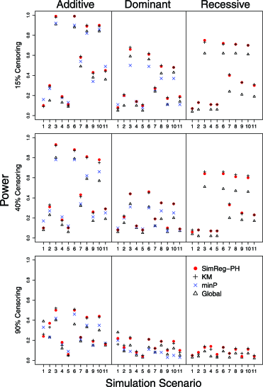
Figure 3: Power when the survival times are generated from the PH model.

5.2 Results of power analyses

The power analyses were performed using the settings specified in Table 2. The results were based on 100 replications under each scenario. Figure 3 shows the power when the survival times were generated from the PH model. We first consider the additive mode. When one large-effect causal locus has low MAF and low LD with the other markers (e.g., Scenarios 1, 5 and 11), minP tends to have the highest power independent of the censoring proportion. The good performance of minP is not unexpected in these scenarios because the overall association of the gene was driven by a single large-effect locus, for which the majority of the other SNPs did not carry much information. As a result, there is no power gain when borrowing information from other SNPs, which is what SimReg-PH does. However, the power gain of minP over other methods generally diminishes as the number of causal loci increases (e.g., Scenarios 5 to 10). In scenarios where the marker set is not dominated by a single causal locus of low MAF and low LD, SimReg-PH showed comparable or higher power. As expected, KM had near identical power as SimReg-PH in all scenarios. In most scenarios, the Global test produces the least amount of power largely due to the over-conservative test size. The overall performance under the dominant mode has a similar trend to that of the additive mode. However, the power of SimReg-PH is comparable to or better power than the power of minP in more cases under the dominant mode than under the additive mode. For the recessive mode, SimReg-PH appears to have better power than the Global test. We did not perform a power analysis for minP because the type I error rates were inflated.

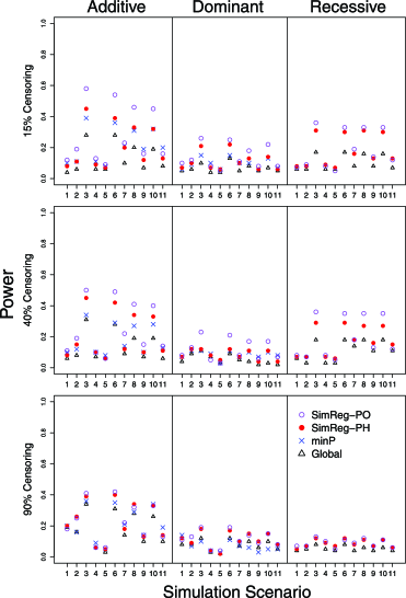
Figure 4: Power when the survival times are generated from the PO model.

Figure 4 shows the power performance when the survival times were generated from the PO model. The power obtained using SimReg-PO is similar to or better than the power obtained using SimReg-PH, indicating that efficiency is gained when the correct model is used. The power gain of SimReg-PO is more substantial when the censoring proportion is low to medium, and the power is comparable to or better power than the minP power in some of those difficult cases, such as Scenario 1.

6 Discussion

In this work we extended the similarity regression (SimReg) approaches, which have shown effectiveness in modeling marker-set effects on binary and continuous outcomes, to survival models to facilitate the assessment of gene or pathway effects on drug responses. The genetic effect is evaluated by assessing the association between the IBS status of a pair of individuals and the covariance of their survival times. We derived the equivalence between the similarity survival regression and a random effects model. The equivalence facilitates the derivation of the score test statistics and unifies the current variance component-based methods. Specifically, the KM approach [Lin et al. (2011)] is equivalent to SimReg-PH when the same kernel function is used to quantify the genetic similarity, $S_{ij}$. The Global test [Goeman et al. (2005)] can be viewed as a special case of SimReg-PH with $S_{ij}=\sum_{m}\mbox{{g}}_{m,i}^{T}\mbox{{g}}_{m,j}$ (i.e., the linear kernel). However, the results of Global and SimReg-PH with linear kernels may be different because different approaches were used to derive the asymptotic distributions of the test statistics. Compared to these existing gene-based approaches, our proposed method has the generality to incorporate a variety of risk models in the class of linear transformation models, and we explicitly constructed the SimReg tests under the PH model and the PO model in this work. We also proposed a resampling approach to obtain the $p$-values that improves the computational efficiency. Finally, we showed that the derived inference procedure is robust against the misspecification of the risk model, which is an attractive feature because the underlying risk model is often unknown. Through simulations, we showed that the power of the SimReg method is comparable to or higher than the power of the minP and Global methods across various scenarios. We also verified that the SimReg-PH test statistics remain valid even if the risk model is misspecified.

In the data application on the VISP study, we illustrated how SimReg can be used to search for genes or pathways that are associated with a time-to-event outcome and confirmed previous findings using this gene-based approach with statistical significance. Although we focused our method development and demonstrated its utility based on pharmacogenetics studies, the proposed method is applicable to other genetic clinical researches or observational studies with time-to-event outcomes. For a pharmacogenetic study with sample sizes 1000, such as the VISP trial, 1000 runs of the SimReg analyses took $\leq$1 hour to complete on an Intel Xeon 3.33 GHz machine with 12 Gb RAM using one processing core. We expect a gene-based whole genome analysis on $\sim$20K genes should be completed in a day using a comparable computing facility. We implemented the proposed methods in R and made it available at the authors’ websites. We are incorporating the software into the SimReg R package.

Motivated by the data application where the risk variant acted recessively, we further investigated the behavior of the gene-based approaches under different modes of inheritance. We found that all of the studied gene-based methods performed appropriately under the additive and dominant modes. However, caution should be used when performing the minimal $p$-value approaches under the recessive mode; the minimal $p$-value approaches had severely inflated type I error rates. The inflation might be related to the extremely rare recessive loci. However, excluding those rare recessive loci is suboptimal because the important signals can be artificially removed and lead to power loss. In contrast, the global test and the similarity regression are not vulnerable to such a situation and appear to be more suitable options given their reasonable performance under the recessive mode.

This work focused on assessing the genetic main effect on drug response in an effort to understand how individual variation affects drug efficacy and toxicity. In pharmacogenetics and personalized medicine, one major topic is to study if the genetic effects are modified by treatments and how the effects differ across treatment options. As observed in the VISP genetic studies, the effect of TCN2 on recurrent stroke risk is restricted to the low-dose treatment. An analysis stratified by treatments allows for the evaluation of such heterogeneous effects between different treatment groups, but its efficiency can be further improved by incorporating the gene-treatment interaction in the regression model. Such an extension is not straightforward because the calculation of the score test requires the variance component estimates for the genetic main effect under a mixed-effects survival model. We are developing further extensions of SimReg to incorporate interaction effects.

Appendix

Derivation of the score statistic $Q_{n}$: Given the working mixed model $H(T_{i})=\gamma^{T}X_{i}+g_{i}+\varepsilon_{i}^{\ast}$, the log-likelihood function of the observed data can be written as

$$l_{n}(\gamma,H,\tau)$$

$$\qquad=\log\int\cdots\int\prod_{i=1}^{n}\bigl{[}\lambda\bigl{\{}H(\tilde{T}_{i})-\gamma^{T}X_{i}-g_{i}\bigr{\}}\bigr{]}^{\delta_{i}}$$

$$\hskip 96.0pt{}\times e^{-\Lambda\{H(\tilde{T}_{i})-\gamma^{T}X_{i}-g_{i}\}}f_{G}(g_{1},\ldots,g_{n})\,dg_{1}\cdots dg_{n},$$

where $\lambda$ and $\Lambda$ are the specified hazard and cumulative hazard functions of $\varepsilon_{i}^{\ast}$, and $f_{G}(g_{1},\ldots,g_{n})$ is the joint density of $g_{1},\ldots,g_{n}$, that is, a multivariate normal density with mean 0 and variance–covariance matrix $\tau S$. Consider the variable transformation $(g^{*}_{1},\ldots,g^{*}_{n})^{\prime}=\tau^{-1/2}S^{-1/2}(g_{1},\ldots,g_{n})^{\prime}$, where $S=S^{1/2}S^{1/2}$. Then $(g^{*}_{1},\ldots,g^{*}_{n})^{\prime}$ follows a standard multivariate normal distribution. The result leads to

$$l_{n}(\gamma,H,\tau)$$

$$\qquad=\log\int\cdots\int\prod_{i=1}^{n}\bigl{[}\lambda\bigl{\{}H(\tilde{T}_{i})-\gamma^{T}X_{i}-\tau^{1/2}S^{1/2}g^{*}_{i}\bigr{\}}\bigr{]}^{\delta_{i}}$$

$$\hskip 96.0pt{}\times e^{-\Lambda\{H(\tilde{T}_{i})-\gamma^{T}X_{i}-\tau^{1/2}S^{1/2}g^{*}_{i}\}}$$

$$\hskip 64.0pt\qquad\quad{}\times f^{*}_{G}\bigl{(}g^{*}_{1},\ldots,g^{*}_{n}\bigr{)}\,dg^{*}_{1}\cdots dg^{*}_{n},$$

where $f^{*}_{G}$ is the density for the standard multivariate normal distribution. After some algebra, we have

$$\frac{1}{n}\frac{\partial l_{n}(\gamma,H,\tau)}{\partial\tau}\bigg{|}_{\tau=0}$$

$$\qquad=\frac{1}{2n}(r_{1},\ldots,r_{n})S(r_{1},\ldots,r_{n})^{T}$$

$$\qquad\quad{}+\frac{1}{2n}\sum_{i=1}^{n}\biggl{[}\frac{\ddot{\lambda}(e_{i})\lambda(e_{i})-\{\dot{\lambda}(e_{i})\}^{2}}{\lambda^{2}(e_{i})}-\dot{\lambda}(e_{i})\biggr{]}s_{i}^{T}s_{i},$$

where $e_{i}=H(\tilde{T}_{i})-\gamma^{T}X_{i}$, $\ddot{\lambda}(\cdot)$ is the second derivative of $\lambda(\cdot)$, $s_{i}$ is the $i$th row of the matrix $S^{1/2}$ and $r_{i}=\int_{0}^{\infty}\dot{\lambda}\{H(t)-\gamma^{T}X_{i}\}/\lambda\{H(t)-\gamma^{T}X_{i}\}\,dM_{i}(t;\break\gamma,H)$. The equality in the above equation is obtained by first taking the derivative of $l_{n}(\gamma,H,\tau)$ with respect to $\tau$ and then deriving its limit as $\tau\rightarrow 0$ using L’Hôpital’s rule. Note that the first term on the right-hand side of the above equation is nonnegative, and the second term converges in probability to a constant as $n$ goes to infinity. In addition, under the null hypothesis, $r_{i}$’s have expectation of 0 at the true values of $\gamma$ and $H$ because they are martingale integrations. Therefore, if the null hypothesis is correct, the first term in the summation should be close to 0. This result motivates us to consider a score test and reject the null hypothesis when the score $(1/n)\partial{l_{n}(\hat{\gamma},\hat{H},\tau)/\partial\tau}|_{\tau=0}$ is bigger than some value, where $\hat{\gamma}$ and $\hat{H}$ are the estimates of $\gamma$ and $H$, respectively, under the null model. It is asymptotically equivalent to consider the test statistic $Q_{n}=n^{-1}(\hat{r}_{1},\ldots,\hat{r}_{n})S(\hat{r}_{1},\ldots,\hat{r}_{n})^{T}$ and reject the null hypothesis when $Q_{n}>c_{\alpha}$, where $c_{\alpha}$ is the critical value for a level-$\alpha$ test.

Null distribution of the score statistic $Q_{n}$: Here, we consider the estimators $\hat{\gamma}$ and $\hat{H}(\cdot)$ obtained via the martingale-based estimating equations for the standard linear transformation model [Chen, Jin and Ying (2002)] under the null hypothesis. Note that $Q_{n}=(n^{-1/2}\sum_{i=1}^{n}\hat{r}_{i}s_{i})^{T}(n^{-1/2}\sum_{i=1}^{n}\hat{r}_{i}s_{i})$. Let $\gamma_{0}$ and $H_{0}$ denote the true values of $\gamma$ and $H$, respectively, in the null model. Based on the derivations given in Chen, Jin and Ying (2002), we have the following asymptotic representations:

$$\sqrt{n}(\hat{\gamma}-\gamma_{0}) = -A^{-1}\frac{1}{\sqrt{n}}\sum_{i=1}^{n}\int_{0}^{\infty}\bigl{\{}X_{i}-\mu_{X}(t)\bigr{\}}\,dM_{i}(t;\gamma_{0},H_{0})+o_{p}(1),$$

$$\sqrt{n}\bigl{\{}\hat{H}(t)-H_{0}(t)\bigr{\}} = -b_{1}(t)^{T}A^{-1}\frac{1}{\sqrt{n}}\sum_{i=1}^{n}\int_{0}^{\infty}\bigl{\{}X_{i}-\mu_{X}(t)\bigr{\}}\,dM_{i}(t;\gamma_{0},H_{0})$$

$${}+\frac{1}{\sqrt{n}}\sum_{i=1}^{n}\int_{0}^{t}\phi(t,s)\,dM_{i}(s;\gamma_{0},H_{0})+o_{p}(1).$$

The definitions of $A$, $\mu_{X}(\cdot)$, $b_{1}(\cdot)$ and $\phi(\cdot,\cdot)$ can be found in Chen, Jin and Ying (2002). By the Taylor expansion, we can show that

$$\frac{1}{\sqrt{n}}\sum_{i=1}^{n}\hat{r}_{i}s_{i}\rightarrow_{d}N(0,\Sigma),$$

as $n\rightarrow\infty$, where $\Sigma=E(\psi_{i}\psi_{i}^{T})$ and

$$\psi_{i} = \biggl{[}\delta_{i}\frac{\dot{\lambda}\{H_{0}(\tilde{T}_{i})-\gamma_{0}^{T}X_{i}\}}{\lambda\{H_{0}(\tilde{T}_{i})-\gamma_{0}^{T}X_{i}\}}-\lambda\bigl{\{}H_{0}(\tilde{T}_{i})-\gamma_{0}^{T}X_{i}\bigr{\}}\biggr{]}s_{i}$$

$${}-(B_{1}-B_{2})A^{-1}\int_{0}^{\infty}\bigl{\{}X_{i}-\mu_{X}(t)\bigr{\}}\,dM_{i}(t;\gamma_{0},H_{0})$$

$${}-\int_{0}^{\infty}b_{2}(t)\,dM_{i}(t;\gamma_{0},H_{0}).$$

Here

$$B_{1} = \lim_{n\rightarrow\infty}\frac{1}{n}\sum_{i=1}^{n}s_{i}X_{i}^{T}\bigl{[}\dot{\lambda}\bigl{\{}H_{0}(\tilde{T}_{i})-\gamma_{0}^{T}X_{i}\bigr{\}}$$

$$\hskip 73.0pt{}-\delta_{i}\bigl{(}\ddot{\lambda}\bigl{\{}H_{0}(\tilde{T}_{i})-\gamma_{0}^{T}X_{i}\bigr{\}}\lambda\bigl{\{}H_{0}(\tilde{T}_{i})-\gamma_{0}^{T}X_{i}\bigr{\}}$$

$$\hskip 159.0pt{}-\bigl{(}\dot{\lambda}\bigl{\{}H_{0}(\tilde{T}_{i})-\gamma_{0}^{T}X_{i}\bigr{\}}\bigr{)}^{2}\bigr{)}$$

$$\hskip 172.0pt/\bigl{(}\lambda\bigl{\{}H_{0}(\tilde{T}_{i})-\gamma_{0}^{T}X_{i}\bigr{\}}\bigr{)}^{2}\bigr{]},$$

$$B_{2} = \lim_{n\rightarrow\infty}\frac{1}{n}\sum_{i=1}^{n}s_{i}b_{1}(\tilde{T}_{i})^{T}\bigl{[}\dot{\lambda}\bigl{\{}H_{0}(\tilde{T}_{i})-\gamma_{0}^{T}X_{i}\bigr{\}}$$

$$\hskip 93.0pt{}-\delta_{i}\bigl{(}\ddot{\lambda}\bigl{\{}H_{0}(\tilde{T}_{i})-\gamma_{0}^{T}X_{i}\bigr{\}}\lambda\bigl{\{}H_{0}(\tilde{T}_{i})-\gamma_{0}^{T}X_{i}\bigr{\}}$$

$$\hskip 177.0pt{}-\bigl{(}\dot{\lambda}\bigl{\{}H_{0}(\tilde{T}_{i})-\gamma_{0}^{T}X_{i}\bigr{\}}\bigr{)}^{2}\bigr{)}$$

$$\hskip 189.0pt{}/{\bigl{(}\lambda\bigl{\{}H_{0}(\tilde{T}_{i})-\gamma_{0}^{T}X_{i}\bigr{\}}\bigr{)}^{2}}\bigr{]},$$

$$b_{2}(t) = \lim_{n\rightarrow\infty}\frac{1}{n}\sum_{i=1}^{n}s_{i}I(\tilde{T}_{i}\geq t)$$

$$\hskip 47.0pt{}\times\phi(\tilde{T}_{i},t)\bigl{[}\dot{\lambda}\bigl{\{}H_{0}(\tilde{T}_{i})-\gamma_{0}^{T}X_{i}\bigr{\}}$$

$$\hskip 98.0pt{}-\delta_{i}\bigl{(}\ddot{\lambda}\bigl{\{}H_{0}(\tilde{T}_{i})-\gamma_{0}^{T}X_{i}\bigr{\}}\lambda\bigl{\{}H_{0}(\tilde{T}_{i})-\gamma_{0}^{T}X_{i}\bigr{\}}$$

$$\hskip 182.0pt{}-\bigl{(}\dot{\lambda}\bigl{\{}H_{0}(\tilde{T}_{i})-\gamma_{0}^{T}X_{i}\bigr{\}}\bigr{)}^{2}\bigr{)}$$

$$\hskip 194.0pt/{\bigl{(}\lambda\bigl{\{}H_{0}(\tilde{T}_{i})-\gamma_{0}^{T}X_{i}\bigr{\}}\bigr{)}^{2}}\bigr{]}.$$

Therefore, $Q_{n}$ converges in distribution to a weighted $\chi^{2}$ distribution: $\sum_{k=1}^{d}\xi_{k}\chi_{1,k}^{2}$, where $\chi_{1,1}^{2},\ldots,\chi_{1,d}^{2}$ are $d$ independently and identically distributed $\chi^{2}$ random variables with degree freedom of 1, and $\xi_{1},\ldots,\xi_{d}$ are the $d$ nonzero eigenvalues of the matrix $\Sigma$. To obtain the critical value, $c_{\alpha}$, of the limiting weighted $\chi^{2}$ distribution, we use a numerical method. Specifically, we first obtain a consistent estimator, $\hat{\Sigma}$, of $\Sigma$ using the usual plug-in method and compute the nonzero eigenvalues $\hat{\xi}_{1},\ldots,\hat{\xi}_{d}$ of the matrix $\hat{\Sigma}$. Next we generate a large set (e.g., 10,000 sets) of independent and identically distributed random variables $\chi_{1,1}^{2},\ldots,\chi_{1,d}^{2}$. For each set of $\chi^{2}$ random variables, we compute $\sum_{k=1}^{d}\hat{\xi}_{k}\chi_{1,k}^{2}$. We can then estimate $c_{\alpha}$ by the upper $\alpha$-quantile of $\sum_{k=1}^{d}\hat{\xi}_{k}\chi_{1,k}^{2}$’s and the associated $p$-value of the score test can be computed accordingly.

References

- Afman et al. (2003) {barticle}[pbm] \bauthor\bsnmAfman, \bfnmLydia A.\binitsL. A., \bauthor\bsnmLievers, \bfnmKarin J. A.\binitsK. J. A., \bauthor\bsnmKluijtmans, \bfnmLeo A. J.\binitsL. A. J., \bauthor\bsnmTrijbels, \bfnmFrans J. M.\binitsF. J. M. and \bauthor\bsnmBlom, \bfnmHenk J.\binitsH. J. (\byear2003). \btitleGene–gene interaction between the cystathionine beta-synthase 31 base pair variable number of tandem repeats and the methylenetetrahydrofolate reductase 677CT polymorphism on homocysteine levels and risk for neural tube defects. \bjournalMol. Genet. Metab. \bvolume78 \bpages211–215. \bidissn=1096-7192, pii=S1096719203000210, pmid=12649066 \bptokimsref\endbibitem
- Beckmann et al. (2005) {barticle}[pbm] \bauthor\bsnmBeckmann, \bfnmL.\binitsL., \bauthor\bsnmThomas, \bfnmD. C.\binitsD. C., \bauthor\bsnmFischer, \bfnmC.\binitsC. and \bauthor\bsnmChang-Claude, \bfnmJ.\binitsJ. (\byear2005). \btitleHaplotype sharing analysis using mantel statistics. \bjournalHum. Hered. \bvolume59 \bpages67–78. \biddoi=10.1159/000085221, issn=0001-5652, pii=85221, pmid=15838176 \bptokimsref\endbibitem
- Bennett (1983) {barticle}[pbm] \bauthor\bsnmBennett, \bfnmS.\binitsS. (\byear1983). \btitleAnalysis of survival data by the proportional odds model. \bjournalStat. Med. \bvolume2 \bpages273–277. \bidissn=0277-6715, pmid=6648142 \bptokimsref\endbibitem
- Cai, Tonini and Lin (2011) {barticle}[mr] \bauthor\bsnmCai, \bfnmTianxi\binitsT., \bauthor\bsnmTonini, \bfnmGiulia\binitsG. and \bauthor\bsnmLin, \bfnmXihong\binitsX. (\byear2011). \btitleKernel machine approach to testing the significance of multiple genetic markers for risk prediction. \bjournalBiometrics \bvolume67 \bpages975–986. \biddoi=10.1111/j.1541-0420.2010.01544.x, issn=0006-341X, mr=2829272 \bptokimsref\endbibitem
- Chen, Jin and Ying (2002) {barticle}[mr] \bauthor\bsnmChen, \bfnmKani\binitsK., \bauthor\bsnmJin, \bfnmZhezhen\binitsZ. and \bauthor\bsnmYing, \bfnmZhiliang\binitsZ. (\byear2002). \btitleSemiparametric analysis of transformation models with censored data. \bjournalBiometrika \bvolume89 \bpages659–668. \biddoi=10.1093/biomet/89.3.659, issn=0006-3444, mr=1929170 \bptokimsref\endbibitem
- Cheng, Wei and Ying (1995) {barticle}[mr] \bauthor\bsnmCheng, \bfnmS. C.\binitsS. C., \bauthor\bsnmWei, \bfnmL. J.\binitsL. J. and \bauthor\bsnmYing, \bfnmZ.\binitsZ. (\byear1995). \btitleAnalysis of transformation models with censored data. \bjournalBiometrika \bvolume82 \bpages835–845. \biddoi=10.1093/biomet/82.4.835, issn=0006-3444, mr=1380818 \bptokimsref\endbibitem
- Cox (1972) {barticle}[mr] \bauthor\bsnmCox, \bfnmD. R.\binitsD. R. (\byear1972). \btitleRegression models and life-tables. \bjournalJ. R. Stat. Soc. Ser. B Stat. Methodol. \bvolume34 \bpages187–220. \bidissn=0035-9246, mr=0341758 \bptnotecheck related \bptokimsref\endbibitem
- Duchesne and Lafaye De Micheaux (2010) {barticle}[mr] \bauthor\bsnmDuchesne, \bfnmPierre\binitsP. and \bauthor\bsnmLafaye De Micheaux, \bfnmPierre\binitsP. (\byear2010). \btitleComputing the distribution of quadratic forms: Further comparisons between the Liu–Tang–Zhang approximation and exact methods. \bjournalComput. Statist. Data Anal. \bvolume54 \bpages858–862. \biddoi=10.1016/j.csda.2009.11.025, issn=0167-9473, mr=2580921 \bptokimsref\endbibitem
- Elston et al. (2000) {barticle}[pbm] \bauthor\bsnmElston, \bfnmR. C.\binitsR. C., \bauthor\bsnmBuxbaum, \bfnmS.\binitsS., \bauthor\bsnmJacobs, \bfnmK. B.\binitsK. B. and \bauthor\bsnmOlson, \bfnmJ. M.\binitsJ. M. (\byear2000). \btitleHaseman and Elston revisited. \bjournalGenet. Epidemiol. \bvolume19 \bpages1–17. \biddoi=10.1002/1098-2272(200007)19:1¡1::AID-GEPI1¿3.0.CO;2-E, issn=0741-0395, pii=10.1002/1098-2272(200007)19:1¡1::AID-GEPI1¿3.0.CO;2-E, pmid=10861893 \bptokimsref\endbibitem
- Giusti et al. (2010) {barticle}[auto:STB—2014/02/12—14:17:21] \bauthor\bsnmGiusti, \bfnmB.\binitsB., \bauthor\bsnmSaracinim, \bfnmC.\binitsC., \bauthor\bsnmBolli, \bfnmP.\binitsP., \bauthor\bsnmMagi, \bfnmA.\binitsA., \bauthor\bsnmMartinelli, \bfnmI.\binitsI., \bauthor\bsnmPeyvandi, \bfnmF.\binitsF., \bauthor\bsnmRasura, \bfnmM.\binitsM., \bauthor\bsnmVolpe, \bfnmM.\binitsM., \bauthor\bsnmLotta, \bfnmL. A.\binitsL. A., \bauthor\bsnmRubattu, \bfnmS.\binitsS., \bauthor\bsnmMannucci, \bfnmP. M.\binitsP. M. and \bauthor\bsnmAbbate, \bfnmR.\binitsR. (\byear2010). \btitleEarly-onset ischaemic stroke: Analysis of 58 polymorphisms in 17 genes involved in methionine metabolism. \bjournalThrombosis and Haemostasis \bvolume104 \bpages231–242. \bptokimsref\endbibitem
- Goeman et al. (2005) {barticle}[pbm] \bauthor\bsnmGoeman, \bfnmJelle J.\binitsJ. J., \bauthor\bsnmOosting, \bfnmJan\binitsJ., \bauthor\bsnmCleton-Jansen, \bfnmAnne-Marie\binitsA.-M., \bauthor\bsnmAnninga, \bfnmJakob K.\binitsJ. K. and \bauthor\bparticlevan \bsnmHouwelingen, \bfnmHans C.\binitsH. C. (\byear2005). \btitleTesting association of a pathway with survival using gene expression data. \bjournalBioinformatics \bvolume21 \bpages1950–1957. \biddoi=10.1093/bioinformatics/bti267, issn=1367-4803, pii=bti267, pmid=15657105 \bptokimsref\endbibitem
- Goldstein (2005) {barticle}[auto:STB—2014/02/12—14:17:21] \bauthor\bsnmGoldstein, \bfnmD. B.\binitsD. B. (\byear2005). \btitleThe genetics of human drug response. \bjournalPhilosophical Transactions of the Royal Society B: Biological Sciences \bvolume360 \bpages1571–1572. \bptokimsref\endbibitem
- Goldstein, Tate and Sisodiya (2003) {barticle}[pbm] \bauthor\bsnmGoldstein, \bfnmDavid B.\binitsD. B., \bauthor\bsnmTate, \bfnmSarah K.\binitsS. K. and \bauthor\bsnmSisodiya, \bfnmSanjay M.\binitsS. M. (\byear2003). \btitlePharmacogenetics goes genomic. \bjournalNat. Rev. Genet. \bvolume4 \bpages937–947. \biddoi=10.1038/nrg1229, issn=1471-0056, pii=nrg1229, pmid=14631354 \bptokimsref\endbibitem
- Haseman and Elston (1972) {barticle}[pbm] \bauthor\bsnmHaseman, \bfnmJ. K.\binitsJ. K. and \bauthor\bsnmElston, \bfnmR. C.\binitsR. C. (\byear1972). \btitleThe investigation of linkage between a quantitative trait and a marker locus. \bjournalBehav. Genet. \bvolume2 \bpages3–19. \bidissn=0001-8244, pmid=4157472 \bptokimsref\endbibitem
- Hsu, Sides and Mychaleckyj (2011) {barticle}[auto:STB—2014/02/12—14:17:21] \bauthor\bsnmHsu, \bfnmF. C.\binitsF. C., \bauthor\bsnmSides, \bfnmE. G.\binitsE. G. and \bauthor\bsnmMychaleckyj, \bfnmJ. C.\binitsJ. C.\betalet al. (\byear2011). \btitleA Transcobalamin 2 gene variant associated with post-stroke homocysteine modifies recurrent stroke risk. \bjournalNeurology \bvolume77 \bpages1543–1550. \bptokimsref\endbibitem
- Li and Luan (2005) {barticle}[auto:STB—2014/02/12—14:17:21] \bauthor\bsnmLi, \bfnmH.\binitsH. and \bauthor\bsnmLuan, \bfnmY.\binitsY. (\byear2005). \btitleBoosting proportional hazards models using smoothing spline, with application to high-dimensional microarray data. \bjournalBiostatistics \bvolume21 \bpages2403–2409. \bptokimsref\endbibitem
- Lin and Wei (1989) {barticle}[mr] \bauthor\bsnmLin, \bfnmD. Y.\binitsD. Y. and \bauthor\bsnmWei, \bfnmL. J.\binitsL. J. (\byear1989). \btitleThe robust inference for the Cox proportional hazards model. \bjournalJ. Amer. Statist. Assoc. \bvolume84 \bpages1074–1078. \bidissn=0162-1459, mr=1134495 \bptokimsref\endbibitem
- Lin and Schaid (2009) {barticle}[pbm] \bauthor\bsnmLin, \bfnmWan-Yu\binitsW.-Y. and \bauthor\bsnmSchaid, \bfnmDaniel J.\binitsD. J. (\byear2009). \btitlePower comparisons between similarity-based multilocus association methods, logistic regression, and score tests for haplotypes. \bjournalGenet. Epidemiol. \bvolume33 \bpages183–197. \biddoi=10.1002/gepi.20364, issn=1098-2272, mid=NIHMS106122, pmcid=2674317, pmid=18814307 \bptokimsref\endbibitem
- Lin et al. (2011) {barticle}[pbm] \bauthor\bsnmLin, \bfnmXinyi\binitsX., \bauthor\bsnmCai, \bfnmTianxi\binitsT., \bauthor\bsnmWu, \bfnmMichael C.\binitsM. C., \bauthor\bsnmZhou, \bfnmQian\binitsQ., \bauthor\bsnmLiu, \bfnmGeoffrey\binitsG., \bauthor\bsnmChristiani, \bfnmDavid C.\binitsD. C. and \bauthor\bsnmLin, \bfnmXihong\binitsX. (\byear2011). \btitleKernel machine SNP-set analysis for censored survival outcomes in genome-wide association studies. \bjournalGenet. Epidemiol. \bvolume35 \bpages620–631. \biddoi=10.1002/gepi.20610, issn=1098-2272, mid=NIHMS308069, pmcid=3373190, pmid=21818772 \bptokimsref\endbibitem
- Low et al. (2011) {barticle}[pbm] \bauthor\bsnmLow, \bfnmHui-Qi\binitsH.-Q., \bauthor\bsnmChen, \bfnmChristopher P. L H.\binitsC. P. L. H., \bauthor\bsnmKasiman, \bfnmKatherine\binitsK., \bauthor\bsnmThalamuthu, \bfnmAnbupalam\binitsA., \bauthor\bsnmNg, \bfnmSeok-Shin\binitsS.-S., \bauthor\bsnmFoo, \bfnmJia-Nee\binitsJ.-N., \bauthor\bsnmChang, \bfnmHui-Meng\binitsH.-M., \bauthor\bsnmWong, \bfnmMeng-Cheong\binitsM.-C., \bauthor\bsnmTai, \bfnmE.-Shyong\binitsE.-S. and \bauthor\bsnmLiu, \bfnmJianjun\binitsJ. (\byear2011). \btitleA comprehensive association analysis of homocysteine metabolic pathway genes in Singaporean Chinese with ischemic stroke. \bjournalPLoS ONE \bvolume6 \bpagese24757. \biddoi=10.1371/journal.pone.0024757, issn=1932-6203, pii=PONE-D-11-08307, pmcid=3174208, pmid=21935458 \bptokimsref\endbibitem
- Moskvina and Schmidt (2008) {barticle}[pbm] \bauthor\bsnmMoskvina, \bfnmValentina\binitsV. and \bauthor\bsnmSchmidt, \bfnmKarl Michael\binitsK. M. (\byear2008). \btitleOn multiple-testing correction in genome-wide association studies. \bjournalGenet. Epidemiol. \bvolume32 \bpages567–573. \biddoi=10.1002/gepi.20331, issn=1098-2272, pmid=18425821 \bptokimsref\endbibitem
- Pearson (1959) {barticle}[mr] \bauthor\bsnmPearson, \bfnmE. S.\binitsE. S. (\byear1959). \btitleNote on an approximation to the distribution of non-central . \bjournalBiometrika \bvolume46 \bpages364. \bidissn=0006-3444, mr=0109380 \bptokimsref\endbibitem
- Pongpanich, Neely and Tzeng (2012) {barticle}[auto:STB—2014/02/12—14:17:21] \bauthor\bsnmPongpanich, \bfnmM.\binitsM., \bauthor\bsnmNeely, \bfnmM.\binitsM. and \bauthor\bsnmTzeng, \bfnmJ. Y.\binitsJ. Y. (\byear2012). \btitleOn the aggregation of multimarker information for marker-set and sequencing data analysis: Genotype collapsing vs. similarity collapsing. \bjournalFrontiers in Statistical Genetics and Methodology \bvolume2 \bpages110. \bptokimsref\endbibitem
- Price et al. (2010) {barticle}[pbm] \bauthor\bsnmPrice, \bfnmAlkes L.\binitsA. L., \bauthor\bsnmKryukov, \bfnmGregory V.\binitsG. V., \bauthor\bparticlede \bsnmBakker, \bfnmPaul I. W.\binitsP. I. W., \bauthor\bsnmPurcell, \bfnmShaun M.\binitsS. M., \bauthor\bsnmStaples, \bfnmJeff\binitsJ., \bauthor\bsnmWei, \bfnmLee-Jen\binitsL.-J. and \bauthor\bsnmSunyaev, \bfnmShamil R.\binitsS. R. (\byear2010). \btitlePooled association tests for rare variants in exon-resequencing studies. \bjournalAm. J. Hum. Genet. \bvolume86 \bpages832–838. \biddoi=10.1016/j.ajhg.2010.04.005, issn=1537-6605, pii=S0002-9297(10)00207-7, pmcid=3032073, pmid=20471002 \bptokimsref\endbibitem
- Qian and Thomas (2001) {barticle}[auto:STB—2014/02/12—14:17:21] \bauthor\bsnmQian, \bfnmD.\binitsD. and \bauthor\bsnmThomas, \bfnmD.\binitsD. (\byear2001). \btitleGenome scan of complex traits by haplotype sharing correlation. \bjournalGenetic Epidemiology \bvolume21 \bpagesS582–S587. \bptokimsref\endbibitem
- Schaid (2010a) {barticle}[auto:STB—2014/02/12—14:17:21] \bauthor\bsnmSchaid, \bfnmD. J.\binitsD. J. (\byear2010a). \btitleGenomic similarity and kernel methods I: Advancements by building on mathematical and statistical foundations. \bjournalHuman Heredity \bvolume70 \bpages109–131. \bptokimsref\endbibitem
- Schaid (2010b) {barticle}[auto:STB—2014/02/12—14:17:21] \bauthor\bsnmSchaid, \bfnmD. J.\binitsD. J. (\byear2010b). \btitleGenomic similarity and kernel methods II: Methods for genomic information. \bjournalHuman Heredity \bvolume70 \bpages132–140. \bptokimsref\endbibitem
- Toole, Malinow and Chambless (2004) {barticle}[auto:STB—2014/02/12—14:17:21] \bauthor\bsnmToole, \bfnmJ. F.\binitsJ. F., \bauthor\bsnmMalinow, \bfnmM. R.\binitsM. R., \bauthor\bsnmChambless, \bfnmL. E.\binitsL. E. \betalet al. (\byear2004). \btitleLowering homocysteine in patients with ischemic stroke to prevent recurrent stroke, myocardial infarction, and death: The Vitamin Intervention for Stroke Prevention (VISP) randomized controlled trial. \bjournalJournal of American Medical Association \bvolume291 \bpages565–575. \bptokimsref\endbibitem
- Tzeng et al. (2003) {barticle}[auto:STB—2014/02/12—14:17:21] \bauthor\bsnmTzeng, \bfnmJ. Y.\binitsJ. Y., \bauthor\bsnmDevlin, \bfnmD.\binitsD., \bauthor\bsnmWasserman, \bfnmL.\binitsL. and \bauthor\bsnmRoeder, \bfnmK.\binitsK. (\byear2003). \btitleOn the identification of disease mutations by the analysis of haplotype similarity and goodness of fit. \bjournalThe American Journal of Human Genetics \bvolume72 \bpages891–902. \bptokimsref\endbibitem
- Tzeng et al. (2009) {barticle}[mr] \bauthor\bsnmTzeng, \bfnmJung-Ying\binitsJ.-Y., \bauthor\bsnmZhang, \bfnmDaowen\binitsD., \bauthor\bsnmChang, \bfnmSheng-Mao\binitsS.-M., \bauthor\bsnmThomas, \bfnmDuncan C.\binitsD. C. and \bauthor\bsnmDavidian, \bfnmMarie\binitsM. (\byear2009). \btitleGene-trait similarity regression for multimarker-based association analysis. \bjournalBiometrics \bvolume65 \bpages822–832. \biddoi=10.1111/j.1541-0420.2008.01176.x, issn=0006-341X, mr=2649855 \bptokimsref\endbibitem
- Tzeng et al. (2011) {barticle}[pbm] \bauthor\bsnmTzeng, \bfnmJung-Ying\binitsJ.-Y., \bauthor\bsnmZhang, \bfnmDaowen\binitsD., \bauthor\bsnmPongpanich, \bfnmMonnat\binitsM., \bauthor\bsnmSmith, \bfnmChris\binitsC., \bauthor\bsnmMcCarthy, \bfnmMark I.\binitsM. I., \bauthor\bsnmSale, \bfnmMichèle M.\binitsM. M., \bauthor\bsnmWorrall, \bfnmBradford B.\binitsB. B., \bauthor\bsnmHsu, \bfnmFang-Chi\binitsF.-C., \bauthor\bsnmThomas, \bfnmDuncan C.\binitsD. C. and \bauthor\bsnmSullivan, \bfnmPatrick F.\binitsP. F. (\byear2011). \btitleStudying gene and gene-environment effects of uncommon and common variants on continuous traits: A marker-set approach using gene-trait similarity regression. \bjournalAm. J. Hum. Genet. \bvolume89 \bpages277–288. \biddoi=10.1016/j.ajhg.2011.07.007, issn=1537-6605, pii=S0002-9297(11)00301-6, pmcid=3155192, pmid=21835306 \bptokimsref\endbibitem
- von Castel-Dunwoody et al. (2005) {barticle}[pbm] \bauthor\bparticlevon \bsnmCastel-Dunwoody, \bfnmKristina M.\binitsK. M., \bauthor\bsnmKauwell, \bfnmGail P. A.\binitsG. P. A., \bauthor\bsnmShelnutt, \bfnmKarla P.\binitsK. P., \bauthor\bsnmVaughn, \bfnmJaimie D.\binitsJ. D., \bauthor\bsnmGriffin, \bfnmElizabeth R.\binitsE. R., \bauthor\bsnmManeval, \bfnmDavid R.\binitsD. R., \bauthor\bsnmTheriaque, \bfnmDouglas W.\binitsD. W. and \bauthor\bsnmBailey, \bfnmLynn B.\binitsL. B. (\byear2005). \btitleTranscobalamin 776CG polymorphism negatively affects vitamin B-12 metabolism. \bjournalAm. J. Clin. Nutr. \bvolume81 \bpages1436–1441. \bidissn=0002-9165, pii=81/6/1436, pmid=15941899 \bptokimsref\endbibitem
- Wang et al. (2004) {barticle}[pbm] \bauthor\bsnmWang, \bfnmJ.\binitsJ., \bauthor\bsnmHuff, \bfnmA. M.\binitsA. M., \bauthor\bsnmSpence, \bfnmJ. D.\binitsJ. D. and \bauthor\bsnmHegele, \bfnmR. A.\binitsR. A. (\byear2004). \btitleSingle nucleotide polymorphism in CTH associated with variation in plasma homocysteine concentration. \bjournalClin. Genet. \bvolume65 \bpages483–486. \biddoi=10.1111/j.1399-0004.2004.00250.x, issn=0009-9163, pii=CGE250, pmid=15151507 \bptokimsref\endbibitem
- Wessel and Schork (2006) {barticle}[pbm] \bauthor\bsnmWessel, \bfnmJennifer\binitsJ. and \bauthor\bsnmSchork, \bfnmNicholas J.\binitsN. J. (\byear2006). \btitleGeneralized genomic distance-based regression methodology for multilocus association analysis. \bjournalAm. J. Hum. Genet. \bvolume79 \bpages792–806. \biddoi=10.1086/508346, issn=0002-9297, pii=S0002-9297(07)60824-6, pmcid=1698575, pmid=17033957 \bptokimsref\endbibitem
- Wu et al. (2011) {barticle}[pbm] \bauthor\bsnmWu, \bfnmMichael C.\binitsM. C., \bauthor\bsnmLee, \bfnmSeunggeun\binitsS., \bauthor\bsnmCai, \bfnmTianxi\binitsT., \bauthor\bsnmLi, \bfnmYun\binitsY., \bauthor\bsnmBoehnke, \bfnmMichael\binitsM. and \bauthor\bsnmLin, \bfnmXihong\binitsX. (\byear2011). \btitleRare-variant association testing for sequencing data with the sequence kernel association test. \bjournalAm. J. Hum. Genet. \bvolume89 \bpages82–93. \biddoi=10.1016/j.ajhg.2011.05.029, issn=1537-6605, pii=S0002-9297(11)00222-9, pmcid=3135811, pmid=21737059 \bptokimsref\endbibitem
- Zeng and Lin (2006) {barticle}[mr] \bauthor\bsnmZeng, \bfnmDonglin\binitsD. and \bauthor\bsnmLin, \bfnmD. Y.\binitsD. Y. (\byear2006). \btitleEfficient estimation of semiparametric transformation models for counting processes. \bjournalBiometrika \bvolume93 \bpages627–640. \biddoi=10.1093/biomet/93.3.627, issn=0006-3444, mr=2261447 \bptokimsref\endbibitem
- Zhong and Chen (2011) {barticle}[mr] \bauthor\bsnmZhong, \bfnmPing-Shou\binitsP.-S. and \bauthor\bsnmChen, \bfnmSong Xi\binitsS. X. (\byear2011). \btitleTests for high-dimensional regression coefficients with factorial designs. \bjournalJ. Amer. Statist. Assoc. \bvolume106 \bpages260–274. \biddoi=10.1198/jasa.2011.tm10284, issn=0162-1459, mr=2816719 \bptokimsref\endbibitem