Abstract

We study dynamics of generalized tachyon scalar field in the framework of teleparallel gravity. This model is an extension of tachyonic teleparallel dark energy model which has been proposed in [26]. In contrast with tachyonic teleparallel dark energy model that has no scaling attractors, here we find some scaling attractors which means that the cosmological coincidence problem can be alleviated. Scaling attractors present for both interacting and non-interacting dark energy, dark matter cases.

PACS numbers: 95.36.+x, 98.80.-k, 04.50.kd
Keywords: Generalized Tachyon Field; Teleparallel gravity; Phase-space analysis.

1 Introduction

The usual proposal to explain the late-time accelerated expansion of our universe is an unknown energy component, dubbed as dark energy. The natural choice and most attractive candidate for dark energy is the cosmological constant but it is not well accepted because of the cosmological constant problem [1] as well as the age problem [2]. Thus, many dynamical dark energy models as alternative possibilities have been proposed. Quintessence, phantom, k-essence, quintom and tachyon field are the most familiar dark energy models in the literature (for reviews on dark energy models, see [3]). The tachyon field arising in the context of string theory [4] and its application in cosmology both as a source of early inflation and late-time cosmic acceleration has been extensively studied [5-8].
The so-called ”Teleparallel Equivalent of General Relativity” or Teleparallel Gravity was first constructed by Einstein [9-12]. In this formulation one uses the curvature-less weitzenbock connection instead of the torsion-less Levi-Civita connection. The relevant lagrangian in teleparallel gravity is the torsion scalar T which is constructed by contraction of the torsion tensor. We recall that the Einstein-Hilbert Lagrangian R is constructed by contraction of the curvature tensor. Since teleparallel gravity with torsion scalar as lagrangian density is completely equivalent to a matter-dominated universe in the framework of general relativity, it can not be accelerated. Thus one should generalize teleparallel gravity either by replacing $T$ with an arbitrary function -the so-called $f(T)$ gravity [13-15] or by adding dark energy into teleparallel gravity allowing also a non-minimal coupling between dark energy and gravity. Note that both approaches are inspired by the similar modifications of general relativity i.e. $f(R)$ gravity [16, 17] and non-minimally coupled dark energy models in the framework of general relativity [18-20].
Recently Geng et al. [21, 22] have included a non-minimal coupling between quintessence and gravity in the context of teleparallel gravity. This theory has been called ”teleparallel dark energy” and its dynamics was studied in [23-25]. Tachyonic teleparallel dark energy is a generalization of teleparallel dark energy by inserting a non-canonical scalar field instead of quintessence in the action [26]. Phase-space analysis of this model has been investigated in [27]. On the other hand, there is no physical argument to exclude the interaction between dark energy and dark matter. The interaction between these completely different component of our universe has same important consequences such as addressing the coincidence problem [28]. In this paper we consider generalized tachyon field as responsible for dark energy in the framework of teleparallel gravity. We will be interested in performing a dynamical analysis of such a model in FRW space time. In such a study we investigate our model for both interacting and non-interacting cases. The basic equations are presented in section 2. In section 3 the evolution equations are translated in the language of the autonomous dynamical system by suitable transformation of the basic variables. Subsection 3.1 deals with phase-space analysis as well as the cosmological implications of the equilibrium points of the model in non-interacting dark energy dark matter case. In subsection 3.2 an interaction between dark energy and dark matter has been considered an critical points and their behavior extracted. Section 5 is devoted to a short summary of our results.

2 Basic Equations

Our model is described by the following action as a generalization of tachyon teleparallel dark energy model [26],

$$S=\int d^{4}xe\Big{[}\mathcal{L}_{T}+\mathcal{L}_{\varphi}+\mathcal{L}_{m}\Big{]},$$

$$\mathcal{L}_{T}=\frac{T}{2\kappa^{2}},$$

$$\mathcal{L}_{\varphi}=\xi f(\varphi)T-V(\varphi)(1-2X)^{\beta},$$ (1)

where $e=det(e_{\,\mu}^{\,i})=\sqrt{-g}$ ($e_{\,\mu}^{\,i}$ are the orthonormal components of the tetrad) while $\frac{T}{2\kappa^{2}}$ is the Lagrangian of teleparallelism with $T$ as the torsion scalar (for an introductory review of teleparallelism see [11]). $\mathcal{L}_{\varphi}$ shows a non-minimal coupling of generalized tachyon field $\varphi$ with gravity in the framework of teleparallel gravity and $X=\frac{1}{2}\partial_{\mu}\varphi\partial^{\mu}\varphi$. The second part in $\mathcal{L}_{\varphi}$ is the Lagrangian density of the generalized tachyon field which has been studied in Ref [29]. $f(\varphi)$ is the non-minimal coupling function, $\xi$ is a dimensionless constant measuring the non-minimal coupling and $\mathcal{L}_{m}$ is the matter Lagrangian. For $\beta=\frac{1}{2}$ our model reduced to tachyonic teleparallel dark energy discussed in [26]. Here we consider the case $\beta=2$ for two reasons. The first is that for arbitrary $\beta$ our equations will be very complicated and one can not solve them analytically and the second is that for $\beta=2$ we will obtain interesting physical results as we will see below.
Furthermore, due to complexity of tachyon dynamics Ref [30] has proposed an approach based on a re-definition of the tachyon field as follows,

$$\varphi\rightarrow\phi=\int d\varphi\sqrt{V(\varphi)}\Leftrightarrow\partial\varphi=\frac{\partial\phi}{\sqrt{V(\phi)}}.$$ (2)

In order to obtain a closed autonomous system and perform the phase-space analysis of the model we apply (2) in (1) for $\beta=2$ that leads to the following action:

$$S=\int d^{4}xe\Big{[}\frac{T}{2\kappa^{2}}+\xi f(\phi)T-V(\phi)\big{(}1-\frac{2X}{V(\phi)}\big{)}^{2}+\mathcal{L}_{m}\Big{]}.$$ (3)

In a spatially-flat FRW space-time,

$$ds^{2}=dt^{2}-a^{2}(t)(dr^{2}+r^{2}d\Omega^{2}),$$ (4)

and a vierbein choice of the form $e^{i}_{\mu}=diag(1,a,a,a)$, the corresponding Friedmann equations are given by,

$$H^{2}=\frac{1}{3}\big{(}\rho_{\phi}+\rho_{m}\big{)},$$ (5)

$$\dot{H}=-\frac{1}{2}\big{(}\rho_{\phi}+P_{\phi}+\rho_{m}+P_{m}\big{)},$$ (6)

where $H=\frac{\dot{a}}{a}$ is the Hubble parameter and a dot stands for the derivative with respect to the cosmic time $t$. In these equations, $\rho_{m}$ and $P_{m}$ are the matter energy density and pressure respectively.
The effective energy density and pressure of generalized tachyon dark energy read,

$$\rho_{\phi}=V(\phi)+2\dot{\phi}^{2}-3\frac{\dot{\phi}^{4}}{V(\phi)}-6\xi H^{2}f(\phi),$$ (7)

and

$$P_{\phi}=-V(\phi)+2\xi\big{(}3H^{2}+2\dot{H}\big{)}f(\phi)+10\xi Hf_{,\phi}\dot{\phi}+\dot{\phi}^{2}\big{(}2-\frac{\dot{\phi}^{2}}{V(\phi)}\big{)},$$ (8)

where $f_{,\phi}=\frac{df}{d\phi}$.
The equation of motion of the scalar field can be obtained by variation of the action (3) with respect to $\phi$,

$$\ddot{\phi}+3\mu^{-2}\nu^{2}H\dot{\phi}+\frac{1}{4}\nu^{2}\big{(}1+\frac{3\dot{\phi}^{4}}{V^{2}(\phi)}\big{)}V_{,\phi}+6\xi\nu^{2}H^{2}f_{,\phi}=-\frac{Q}{\dot{\phi}},$$ (9)

with $Q$ a general interaction coupling term between dark energy and dark matter, $\mu=\frac{1}{\sqrt{1-\frac{2X}{V}}}$ and $\nu=\frac{1}{\sqrt{1-\frac{6X}{V}}}$. In (7), (8) and (9) we have used the useful relation,

$$T=-6H^{2},$$ (10)

which simply arises from the calculation of torsion scalar for the FRW metric (4). The scalar field evolution (9) expresses the continuity equation for the field and matter as follows

$$\dot{\rho}_{\phi}+3H(1+\omega_{\phi})\rho_{\phi}=-Q,$$ (11)

$$\dot{\rho}_{m}+3H(1+\omega_{m})\rho_{m}=Q,$$ (12)

where $\omega_{\phi}=\frac{P_{\phi}}{\rho_{\phi}}$ is the equation of state parameter of dark energy which is attributed to the scalar field $\phi$. The barotropic index is defined by $\gamma\equiv 1+\omega_{m}$ with $0<\gamma<2$.
Although, dynamics of tachyonic teleparallel dark energy has been studied in [27], no scaling attractors found. Here we are going to perform a phase-space analysis of generalized tachyonic teleparallel dark energy and as we will see below some interesting scaling attractors appear in such theory.

3 Cosmological Dynamics

In order to perform phase-space and stability analysis of the model, we introduce the following auxiliary variables:

$$x\equiv\frac{\dot{\phi}}{\sqrt{V}},\,\,\,y\equiv\frac{\sqrt{V}}{\sqrt{3}H},\,\,\,u\equiv\sqrt{f}.$$ (13)

The auxiliary variables allow us to straightforwardly obtain the density parameter of dark energy and dark matter

$$\Omega_{\phi}\equiv\frac{\rho_{\phi}}{3H^{2}}=\mu^{-2}y^{2}\big{(}1+3x^{2}\big{)}-2\xi u^{2},$$ (14)

$$\Omega_{m}\equiv\frac{\rho_{m}}{3H^{2}}=1-\Omega_{\phi},$$ (15)

while the equation of state of the field reads

$$\omega_{\phi}\equiv\frac{P_{\phi}}{\rho_{\phi}}$$

$$=\frac{-\mu^{-4}y^{2}+2\xi u\big{[}\frac{5\sqrt{3}}{3}\alpha xy+u(1-\frac{2}{3}s)\big{]}}{\mu^{-2}y^{2}\big{(}1+3x^{2}\big{)}-2\xi u^{2}},$$ (16)

where $\alpha\equiv\frac{f_{,\phi}}{\sqrt{f}}$ and

$$s=-\frac{\dot{H}}{H^{2}}=(2\xi u^{2}+1)^{-1}\Big{[}5\sqrt{3}\alpha\xi uxy+6\mu^{-2}x^{2}y^{2}-\frac{3}{2}\gamma\mu^{-2}y^{2}\big{(}1+3x^{2}\big{)}\Big{]}+\frac{3\gamma}{2}.$$ (17)

Another quantities with great physical significance namely the total equation of state parameter and the deceleration parameter are given by

$$\omega_{tot}\equiv\frac{P_{\phi}+P_{m}}{\rho_{\phi}+\rho_{m}}=\mu^{-2}y^{2}\big{(}4x^{2}-\gamma(1+3x^{2})\big{)}+2\xi u\big{[}\frac{5\sqrt{3}}{3}\alpha xy+u(\gamma-\frac{2}{3}s)\big{]}+\gamma-1,$$ (18)

and

$$q\equiv-1-\frac{\dot{H}}{H^{2}}=\frac{1}{2}+\frac{3}{2}\omega_{tot}$$

$$=\frac{3}{2}\mu^{-2}y^{2}\big{(}4x^{2}-\gamma(1+3x^{2})\big{)}+\xi u\big{[}5\sqrt{3}\alpha xy+u(3\gamma-2s)\big{]}+\frac{3\gamma}{2}-1.$$ (19)

Using auxiliary variables (13) the evolution equations (5), (6) and (9) can be recast as a dynamical system of ordinary differential equations

$$x^{\prime}=\frac{\sqrt{3}}{2}\big{[}\lambda x^{2}y+\frac{1}{2}\lambda\nu^{2}(1+3x^{4})y-4\alpha\xi\nu^{2}uy^{-1}-2\sqrt{3}\mu^{-2}\nu^{2}x\big{]}-\hat{Q},$$ (20)

$$y^{\prime}=\Big{(}-\frac{\sqrt{3}}{2}\lambda xy+s\Big{)}y,$$ (21)

$$u^{\prime}=\frac{\sqrt{3}\alpha xy}{2},$$ (22)

where $\hat{Q}=\frac{Q}{\dot{\phi}H\sqrt{V(\phi)}}$, $\lambda\equiv-\frac{V_{,\phi}}{\kappa V}$ and prime in equations (20)-(22) denotes differentiation with respect to the so-called e-folding time $N=\ln a$.
From now we concentrate on exponential scalar field potential of the form $V=V_{0}e^{-k\lambda\phi}$ and the non-minimal coupling function of the form $f(\phi)\propto\phi^{2}$. These choices lead to constant $\lambda$ and $\alpha$ respectively.
The next step is the introduction of interaction term $Q$ to obtain an autonomous system out of equations (20)-(22). The fixed points $(x_{c},y_{c},u_{c})$ for which $x^{\prime}=y^{\prime}=u^{\prime}=0$ depend on the choice of the interaction term $Q$ and two general possibilities will be treated in the sequel. The stability of the system at a fixed point can be obtained from the analysis of the determinant and trace of the perturbation matrix $M$. Such a matrix can be constructed by substituting linear perturbations $x\rightarrow x_{c}+\delta x,y\rightarrow y_{c}+\delta y$ and $u\rightarrow u_{c}+\delta u$ about the critical point $(x_{c},y_{c},u_{c})$ into the autonomous system (20)-(22). The $3\times 3$ matrix $M$ of the linearized perturbation equations of the autonomous system is shown in appendix A. Therefor, for each critical point we examine the sign of the real part of the eigenvalues of $M$. According to the usual dynamical system analysis, if the eigenvalues are real and have opposite signs, the corresponding critical point is a saddle point. A fixed point is unstable if the eigenvalues are positive and it is stable for negative real part of the eigenvalues.
In the following subsections we will study the dynamics of generalized tachyon field with different interaction term $Q$. Without lose of generality we assume $\gamma=1$ for simplicity.

3.1 The case for $Q=0$

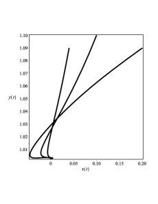
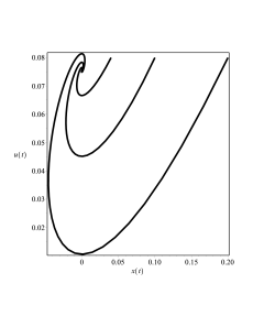
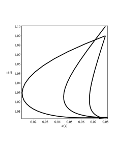
Figure 1: From left to right, the projections of the phase-space trajectories on the $x-y$, $x-u$ and $u-y$ planes with $\xi=0.5$, $\lambda=-0.6$ and $\alpha=-2$ for $Q=0$. For these values of the parameters, point $A_{1}$ is a stable attractor of the model.

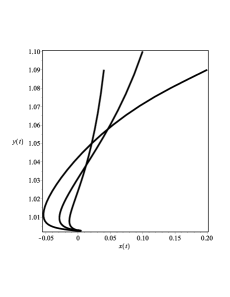
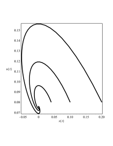
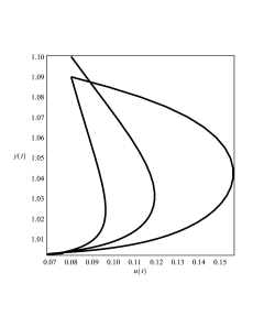
Figure 2: From left to right, the projections of the phase-space trajectories on the $x-y$, $x-u$ and $u-y$ planes with $\xi=0.5$, $\lambda=0.6$ and $\alpha=2$ for $Q=0$. For these values of the parameters, point $A_{2}$ is a stable attractor of the model.

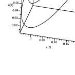
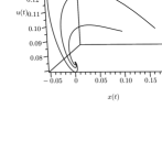
Figure 3: 3-dimensional phase-space trajectories of the model for $Q=0$ with stable attractors $A_{1}$ (left) and $A_{2}$ (right) . The values of the parameters are those mentioned in figure 1 and 2 respectively.

The first case $Q=0$ clearly means there is no interaction between dark energy and background matter. In this case, there are two critical points presented in Table 1. From equations (14) and (16) one can obtain the corresponding values of density parameter $\Omega_{\phi}$ and equation of state of dark energy $\omega_{\phi}$ at each point. Also, using equation (19) we can find the condition required for acceleration $(q<0)$ at each point. These parameters and conditions have been shown in Table 1. The stability and existence conditions of critical points $A_{10}$ and $A_{2}$ are presented in Table 2. We mention that the corresponding eigenvalues of perturbation matrix $M$ at critical points $A_{10}$ and $A_{2}$ are considerably involved and here we do not present their explicit expressions but we can find sign of them numerically.
Critical point $A_{1}$: This critical point is a scaling attractor if $\xi>0$, $\alpha<0$ and $\lambda<0$. Thus, it can give the hope alleviate the cosmological coincidence problem. $A_{1}$ is a saddle point for $\alpha>0$ and $\frac{\xi}{\lambda}>0$.
Critical point $A_{2}$: $A_{2}$ can also be a scaling attractor of the model or a saddle point under the same conditions as for $A_{1}$.
In figure 1 we have chosen the values of the parameters $\xi$, $\lambda$ and $\alpha$, such that $A_{1}$ become a stable attractor of the model. Plots in figure 1 show the phase-space trajectories on $x-y$, $x-u$ and $u-y$ planes from left to right respectively. The same plots are shown in figure 2 for critical point $A_{2}$. Note that the values of the parameter have chosen in the way that $A_{2}$ become a stable point of the model. In figure 3, the corresponding 3 dimensional phase-space trajectories of the model have been presented. One can see that $A_{1}$ and $A_{2}$ are stable attractor of the model in the left and right plots respectively.

label	$(x_{c},y_{c},u_{c})$	$\Omega_{\phi}$	$\omega_{\phi}$	acceleration
$A_{1}$	$0,2\sqrt{\lambda_{1}},\frac{\lambda\lambda_{1}}{2\alpha\xi}$	$4\lambda_{1}\big{(}1-\frac{\lambda^{2}}{8\xi\alpha^{2}}\lambda_{1}\big{)}$	$\frac{16\xi^{2}\alpha^{4}}{\big{(}\lambda^{2}\lambda_{1}^{2}+2\xi\alpha^{2}\big{)}(\lambda^{2}\lambda_{1}-8\xi\alpha^{2})}$	$\begin{array}[]{c}\lambda^{2}>\frac{\xi\alpha^{2}(4\lambda_{1}-1)}{\lambda_{1}^{2}}\big{(}1+\sqrt{1-\frac{32\lambda_{1}}{(1-4\lambda_{1})^{2}}}\big{)}\\ or\\ \lambda^{2}<\frac{\xi\alpha^{2}(4\lambda_{1}-1)}{\lambda_{1}^{2}}\big{(}1-\sqrt{1-\frac{32\lambda_{1}}{(1-4\lambda_{1})^{2}}}\big{)}\\ \end{array}$
$A_{2}$	$0,2\sqrt{\lambda_{2}},\frac{\lambda\lambda_{2}}{2\alpha\xi}$	$4\lambda_{2}\big{(}1-\frac{\lambda^{2}}{8\xi\alpha^{2}}\lambda_{2}\big{)}$	$\frac{16\xi^{2}\alpha^{4}}{\big{(}\lambda^{2}\lambda_{2}^{2}+2\xi\alpha^{2}\big{)}(\lambda^{2}\lambda_{2}-8\xi\alpha^{2})}$	$\begin{array}[]{c}\lambda^{2}>\frac{\xi\alpha^{2}(4\lambda_{2}-1)}{\lambda_{2}^{2}}\big{(}1+\sqrt{1-\frac{32\lambda_{2}}{(1-4\lambda_{2})^{2}}}\big{)}\\ or\\ \lambda^{2}<\frac{\xi\alpha^{2}(4\lambda_{2}-1)}{\lambda_{2}^{2}}\big{(}1-\sqrt{1-\frac{32\lambda_{2}}{(1-4\lambda_{2})^{2}}}\big{)}\\ \end{array}$

Table 1: Location of the critical points and the corresponding values of the dark energy density parameter $\Omega_{\phi}$ and equation of state $\omega_{\phi}$ and the condition required for an accelerating universe for $Q=0$. Here $\lambda_{1}=\frac{\alpha\big{(}4\alpha\xi+\sqrt{16\alpha^{2}\xi^{2}-2\lambda^{2}\xi}\big{)}}{\lambda^{2}}$ and $\lambda_{2}=\frac{\alpha\big{(}4\alpha\xi-\sqrt{16\alpha^{2}\xi^{2}-2\lambda^{2}\xi}\big{)}}{\lambda^{2}}$.

label	stability	existence
$A_{1}$	$\begin{array}[]{c}saddle\,\,point\\ if\,\,\alpha>0\,\,\,and\,\,\,\frac{\xi}{\lambda}>0\\ stable\,\,point\\ if\,\,\xi>0,\,\,\,\alpha<0\,\,\,and\,\,\,\lambda<0\\ \end{array}$	$\begin{array}[]{c}for\,\,all\,\,\xi<0\\ or\\ \xi\geq\frac{\lambda^{2}}{8\alpha^{2}}\\ \end{array}$
$A_{2}$	$\begin{array}[]{c}saddle\,\,point\\ if\,\,\alpha<0\,\,\,and\,\,\,\frac{\xi}{\lambda}<0\\ stable\,\,point\\ if\,\,\xi>0,\,\,\,\alpha>0\,\,\,and\,\,\,\lambda>0\\ \end{array}$	$\begin{array}[]{c}for\,\,all\,\,\xi<0\\ or\\ \xi\geq\frac{\lambda^{2}}{8\alpha^{2}}\\ \end{array}$

Table 2: Stability and existence conditions of the critical points of the model for $Q=0$.

label	$(x_{c},y_{c},u_{c})$	$\Omega_{\phi}$	$\omega_{\phi}$	acceleration
$B_{1}$	$0,\frac{2\sqrt{2\lambda\alpha\xi\theta_{1}}}{\lambda},\theta_{1}$	$2\xi\theta_{1}\big{(}\frac{4\alpha}{\lambda}-\theta_{1})$	$\frac{2\big{(}\xi\theta_{1}^{3}+\frac{2\alpha}{\lambda}\big{)}}{\big{(}\theta_{1}-\frac{4\alpha}{\lambda}\big{)}(1+2\xi\theta_{1}^{2})}$	$\lambda>\frac{8\alpha(\xi\theta_{1}^{2}-1)}{\theta_{1}(8\xi\theta_{1}^{2}+1)}$
$B_{2}$	$0,\frac{2\sqrt{2\lambda\alpha\xi\theta_{2}}}{\lambda},\theta_{2}$	$2\xi\theta_{2}\big{(}\frac{4\alpha}{\lambda}-\theta_{2})$	$\frac{2\big{(}\xi\theta_{2}^{3}+\frac{2\alpha}{\lambda}\big{)}}{\big{(}\theta_{2}-\frac{4\alpha}{\lambda}\big{)}(1+2\xi\theta_{2}^{2})}$	$\lambda>\frac{8\alpha(\xi\theta_{2}^{2}-1)}{\theta_{2}(8\xi\theta_{2}^{2}+1)}$
$B_{3}$	$0,-\frac{2\sqrt{2\lambda\alpha\xi\theta_{1}}}{\lambda},\theta_{1}$	$2\xi\theta_{1}\big{(}\frac{4\alpha}{\lambda}-\theta_{1})$	$\frac{2\big{(}\xi\theta_{1}^{3}+\frac{2\alpha}{\lambda}\big{)}}{\big{(}\theta_{1}-\frac{4\alpha}{\lambda}\big{)}(1+2\xi\theta_{1}^{2})}$	$\lambda>\frac{8\alpha(\xi\theta_{1}^{2}-1)}{\theta_{1}(8\xi\theta_{1}^{2}+1)}$
$B_{4}$	$0,-\frac{2\sqrt{2\lambda\alpha\xi\theta_{2}}}{\lambda},\theta_{2}$	$2\xi\theta_{2}\big{(}\frac{4\alpha}{\lambda}-\theta_{2})$	$\frac{2\big{(}\xi\theta_{2}^{3}+\frac{2\alpha}{\lambda}\big{)}}{\big{(}\theta_{2}-\frac{4\alpha}{\lambda}\big{)}(1+2\xi\theta_{2}^{2})}$	$\lambda>\frac{8\alpha(\xi\theta_{2}^{2}-1)}{\theta_{2}(8\xi\theta_{2}^{2}+1)}$

Table 3: Location of the critical points and the corresponding values of the dark energy density parameter $\Omega_{\phi}$ and equation of state $\omega_{\phi}$ and the condition required for an accelerating universe for $Q=\beta\kappa\rho_{m}\dot{\phi}$. Here $\theta_{1}=\frac{\big{(}4\alpha\xi+\sqrt{16\alpha^{2}\xi^{2}-2\lambda^{2}\xi}\big{)}}{2\lambda\xi}$ and $\theta_{2}=\frac{\big{(}4\alpha\xi-\sqrt{16\alpha^{2}\xi^{2}-2\lambda^{2}\xi}\big{)}}{2\lambda\xi}$.

3.2 The case for $Q=\beta\kappa\rho_{m}\dot{\phi}$

This deals with the most familiar interaction term extensively considered in the literature (see e.g. [25, 31-34]). Here $\hat{Q}$ in terms of auxiliary variables is $\hat{Q}=\sqrt{3}\beta y^{-1}\Omega_{m}$. Inserting such an interaction term in equations (20)-(22) and setting the left hand sides of the equations to zero lead to the critical points $B_{1}$, $B_{2}$, $B_{3}$ and $B_{4}$ presented in Table 3. In the same table we have provided the corresponding values of $\Omega_{\phi}$ and $\omega_{\phi}$ as well as the condition needed for accelerating universe at each fixed points.
The stability and existence conditions for each point presented in Table 4. Since the corresponding eigenvalues of the fixed points are complicated we do not give them here but one can obtain their signs numerically and so concludes about the stability properties of the critical points.
Critical point $B_{1}$: This point exists for $\lambda>0$ and $\xi\geq\frac{\lambda^{2}}{8\alpha^{2}}$. However it is an unstable saddle point.
Critical point $B_{2}$: The critical point $B_{2}$ exists for $\lambda>0$ and $\xi<0$ or $\xi\geq\frac{\lambda^{2}}{8\alpha^{2}}$. This point is a scaling attractor of the model if $\alpha>0$ and $\xi>0$. Figure 4 shows clearly such a behavior of the model for suitable choices of $\xi$, $\lambda$ and $\alpha$.
Critical point $B_{3}$: This point exists for negative values of $\lambda$ and $\xi$ or when $\xi\geq\frac{\lambda^{2}}{8\alpha^{2}}$. Also, it is a stable point if $\alpha<0$ and $\xi>0$ and a saddle point if $\alpha>0$ and $\xi<0$. The values of parameters have been chosen in figure 5 such that $B_{3}$ become a attractor of the model as it is clear from phase-space trajectories.
Critical point $B_{4}$: The point $B_{4}$ exists for $\lambda<0$ and $\xi\geq\frac{\lambda^{2}}{8\alpha^{2}}$. It is a stable point if $\alpha<0$ and $\xi>0$. In figure 6 values of the parameter $\xi$ and $\alpha$ are those satisfy these constraints and so $B_{4}$ becomes a attractor point for phase-plane trajectories. The corresponding 3-dimensional phase-space trajectories of the model for attractor points $B_{2}$ (left), $B_{3}$ (middle) and $B_{4}$ (right) are plotted in figure 7.

label	stability	existence
$B_{1}$	$\begin{array}[]{c}saddle\,\,point\\ if\,\,\alpha>0\,\,\,and\,\,\,\xi>0\\ \end{array}$	$\lambda>0\,\,\,and\,\,\,\xi\geq\frac{\lambda^{2}}{8\alpha^{2}}$
$B_{2}$	$\begin{array}[]{c}saddle\,\,point\\ if\,\,\alpha<0\,\,\,and\,\,\,\xi<0\\ stable\,\,point\\ if\,\,\alpha>0\,\,\,and\,\,\,\xi>0\\ \end{array}$	$\begin{array}[]{c}\lambda>0\,\,\,and\\ for\,\,all\,\,\xi<0\\ or\\ \xi\geq\frac{\lambda^{2}}{8\alpha^{2}}\\ \end{array}$
$B_{3}$	$\begin{array}[]{c}saddle\,\,point\\ if\,\,\alpha>0\,\,\,and\,\,\,\xi<0\\ stable\,\,point\\ if\,\,\alpha<0\,\,\,and\,\,\,\xi>0\\ \end{array}$	$\begin{array}[]{c}\lambda<0\,\,\,and\\ for\,\,all\,\,\xi<0\\ or\\ \xi\geq\frac{\lambda^{2}}{8\alpha^{2}}\\ \end{array}$
$B_{4}$	$\begin{array}[]{c}stable\,\,point\\ if\,\,\alpha<0\,\,\,and\,\,\,\xi>0\\ \end{array}$	$\lambda<0\,\,\,and\,\,\,\xi\geq\frac{\lambda^{2}}{8\alpha^{2}}$

Table 4: Stability and existence conditions of the critical points of the model for $Q=\beta\kappa\rho_{m}\dot{\phi}$.

4 Conclusion

A model of dark energy with non-minimal coupling of quintessence scalar field with gravity in the framework of teleparallel gravity was called teleparallel dark energy [21]. If one replaces quintessence by tachyon field in such a model then tachyonic teleparallel dark energy will be constructed [26].
Moreover, although dark energy and dark matter scale differently with the expansion of our universe, according to the observations [35] we are living in an epoch in which dark energy and dark matter densities are comparable and this is the well-known cosmological coincidence problem [24]. This problem can be alleviated in most dark energy models via the method of scaling solutions in which the density parameters of dark energy and dark matter are both non-vanishing over there.
In this paper we investigated the phase-space analysis of generalized tachyon cosmology in the framework of teleparallel gravity. Our model described by action (1) which generalizes tachyonic teleparallel dark energy model proposed in [26]. We found some scaling attractors in our model for the case $\beta=2$. These scaling attractors are $A_{1}$ and $A_{2}$ when there is no interaction between dark energy and dark matter. $B_{2}$, $B_{3}$ and $B_{4}$ are scaling attractors in the case that dark energy interacts with dark matter through the interacting term $Q=\beta\kappa\rho_{m}\dot{\phi}$. Our results show that generalized tachyon field represents interesting cosmological behavior in compare with ordinary tachyon fields in the framework of teleparallel gravity because there is no scaling attractor in the latter model. So, generalized tachyon field gives us the hope that cosmological coincidence problem can be alleviated without fine-tunings. One can study our model for different kinds of potential and other famous interaction term between dark energy and dark matter.

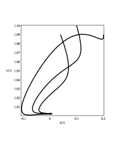
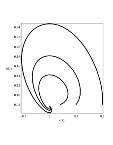
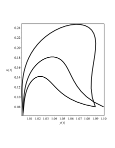
Figure 4: From left to right, the projections of the phase-space trajectories on the $x-y$, $x-u$ and $u-y$ planes with $\xi=0.5$, $\lambda=0.6$, $\alpha=2$ and $\beta=1.5$ for $Q=\beta\kappa\rho_{m}\dot{\phi}$. For these values of the parameters, point $B_{2}$ is a stable attractor of the model.

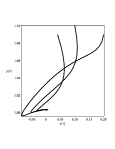
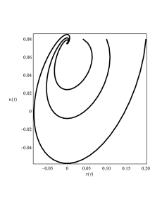
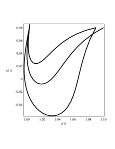
Figure 5: From left to right, the projections of the phase space trajectories on the $x-y$, $x-u$ and $u-y$ planes with $\xi=0.5$, $\lambda=-0.6$, $\alpha=-2$ and $\beta=1.5$ for $Q=\beta\kappa\rho_{m}\dot{\phi}$. For these values of the parameters, point $B_{3}$ is a stable attractor of the model.

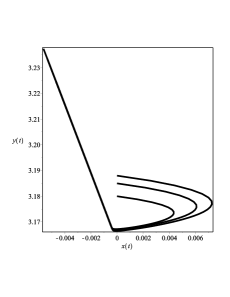
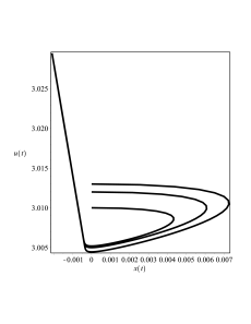
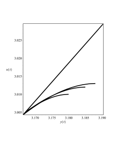
Figure 6: From left to right, the projections of the phase space trajectories on the $x-y$, $x-u$ and $u-y$ planes with $\xi=0.5$, $\lambda=-0.6$, $\alpha=-2$ and $\beta=1.5$ for $Q=\beta\kappa\rho_{m}\dot{\phi}$. For these values of the parameters, point $B_{4}$ is a stable attractor of the model.

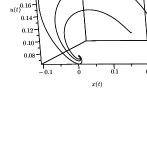
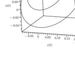
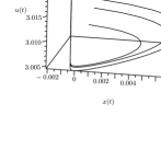
Figure 7: 3-dimensional phase-space trajectories of the model for $Q=\beta\kappa\rho_{m}\dot{\phi}$ with stable attractors $B_{2}$ (left), $B_{3}$ (middle) and $B_{4}$ (right). The values of the parameters are those mentioned in figure 4, 5 and 6 respectively.

5 Appendix: Perturbation Matrix Elements

The elements of $3\times 3$ matrix $M$ of the linearized perturbation equations for the real and physically meaningful critical points $(x_{c},y_{c},u_{c})$ of the autonomous system (20)- (22) read,

$$M_{11}=3\nu_{c}^{2}\Big{(}\frac{\sqrt{3}}{2}\lambda x_{c}y_{c}\big{(}2x_{c}^{2}+\nu_{c}^{2}(1+3x_{c}^{4})\big{)}-6\mu_{c}^{-2}\nu_{c}^{2}x_{c}^{2}-4\sqrt{3}\alpha\xi u_{c}x_{c}\nu_{c}^{2}y_{c}^{-1}\Big{)}+\sqrt{3}\lambda x_{c}y_{c}-3+\mathcal{M}_{11},$$ (23)

$$M_{12}=\frac{\sqrt{3}}{4}\Big{(}\lambda\big{(}2x_{c}^{2}+\nu_{c}^{2}(1+3x_{c}^{4})\big{)}+8\alpha\xi u_{c}\nu_{c}^{2}y_{c}^{-2}\Big{)}+\mathcal{M}_{12},$$ (24)

$$M_{13}=-2\sqrt{3}\alpha\xi\nu_{c}^{2}y_{c}^{-1}+\mathcal{M}_{13},$$ (25)

$$M_{21}=\frac{2y_{c}^{2}\big{(}\sqrt{3}\alpha\xi u_{c}+3x_{c}y_{c}\nu_{c}^{-2}\big{)}}{(2\xi u_{c}^{2}+1)}-\frac{\sqrt{3}\lambda y_{c}^{2}}{2},$$ (26)

$$M_{22}=\frac{2y_{c}\big{(}-\frac{9}{4}\mu_{c}^{-4}y_{c}+5\sqrt{3}\alpha\xi x_{c}u_{c}\big{)}}{(2\xi u_{c}^{2}+1)}-\sqrt{3}\lambda x_{c}y_{c}+\frac{3}{2},$$ (27)

$$M_{23}=\frac{6\xi u_{c}y_{c}^{2}\big{(}-\frac{10\sqrt{3}}{3}\alpha\xi u_{c}x_{c}+\mu_{c}^{-4}y_{c}^{2}\big{)}}{(2\xi u_{c}^{2}+1)^{2}}+\frac{5\sqrt{3}\alpha\xi x_{c}y_{c}^{2}}{2\xi u_{c}^{2}+1},$$ (28)

$$M_{31}=\frac{\sqrt{3}\alpha y_{c}}{2},\,\,\,\,M_{32}=\frac{\sqrt{3}\alpha x_{c}}{2},\,\,\,\,M_{33}=0,$$ (29)

where in the case of $Q=0$ we have $\mathcal{M}_{11}=\mathcal{M}_{12}=\mathcal{M}_{13}=0$ and in the case of $Q=\beta\kappa\rho_{m}\dot{\phi}$ we have

$$\mathcal{M}_{11}=4\sqrt{3}\beta\nu_{c}^{-2}x_{c}y_{c},$$

$$\mathcal{M}_{12}=2\sqrt{3}\beta\mu_{c}^{-2}(1+3x_{c}^{2}),$$

$$\mathcal{M}_{13}=-4\sqrt{3}\beta\xi u_{c}y_{c}^{-1}.$$ (30)

Examining the eigenvalues of the matrix $M$ for each critical point, one determines its stability conditions.

References

• [1] S. Weinberg, Rev. Mod. Phys. 61, 1 (1989); S. M. Carroll, Living Rev. Rel. 4, 1 (2001).
• [2] R.-J. Yang and S. N. Zhang, Mon. Not. R. Astron. Soc. 407, 1835 (2010).
• [3] Y. -F. Cai, E. N. Saridakis, M. R. Setare and J. -Q. Xia, Phys. Rept. 493, 1 (2010); K. Bamba, S. Capozziello, S. Nojiri and S. D. Odintsov, Astrophys. Space Sci. 342, 155 (2012).
• [4] Y. -F. Cai, E. N. Saridakis, M. R. Setare and J. -Q. Xia, Phys. Rept. 493, 1 (2010); K. Bamba, S. Capozziello, S. Nojiri and S. D. Odintsov, Astrophys. Space Sci. 342, 155 (2012).
• [5] A. Sen, Phys. Scripta 117, 70-75 (2005).
• [6] G. W. Gibbons, Phys. Lett. B 537, 1 (2002).
• [7] M. R. Garousi, Nucl. Phys. B 584, 284 (2000).
• [8] A. Sen, Mod. Phys. Lett. A 17, 1797 (2002).
• [9] A. Unzicker and T. Case, [arXiv:physics/0503046].
• [10] K. Hayashi and T. Shirafuji, Phys. Rev. D 19, 3524 (1979) [Addendum-ibid. D 24, 3312 (1982)].
• [11] R. Aldrovandi and J. G. Pereira, Teleparallel Gravity: An Introduction, Springer, Dordrecht (2013).
• [12] J. W. Maluf, Annalen Phys. 525, 339 (2013).
• [13] R. Ferraro and F. Fiorini, Phys. Rev. D 75, 084031 (2007).
• [14] G. R. Bengochea and R. Ferraro, Phys. Rev. D 79, 124019 (2009).
• [15] E. V. Linder, Phys. Rev. D 81, 127301 (2010).
• [16] A. De Felice and S. Tsujikawa, Living Rev. Rel. 13, 3 (2010).
• [17] S. i. Nojiri and S. D. Odintsov, Phys. Rept. 505, 59 (2011).
• [18] B. L. Spokoiny, Phys. Lett. B 147, 39 (1984); F. Perrotta, C. Baccigalupi and S. Matarrese, Phys. Rev. D 61, 023507 (1999).
• [19] V. Faraoni, Phys. Rev. D 62, 023504 (2000); E. Elizalde, S. Nojiri and S. D. Odintsov, Phys. Rev. D 70, 043539 (2004).
• [20] O. Hrycyna and M. Szydlowski, JCAP 0904, 026 (2009); O. Hrycyna and M. Szydlowski, Phys. Rev. D 76, 123510 (2007); R. C. de Souza and G. M. Kremer, Class. Quant. Grav. 26, 135008 (2009); A. A. Sen and N. Chandrachani Devi, Gen. Rel. Grav. 42, 821 (2010).
• [21] C. -Q. Geng, C. -C. Lee, E. N. Saridakis, Y. -P. Wu, Phys. Lett. B 704, 384-387 (2011).
• [22] C. -Q. Geng, C. -C. Lee and E. N. Saridakis, JCAP 1201, 002 (2012).
• [23] C. Xu, E. N. Saridakis and G. Leon, [arXiv:1202.3781 [gr-qc]].
• [24] H. Wei, Phys. Lett. B 712, 430 (2012).
• [25] G. Otalora, JCAP 1307, 044 (2013).
• [26] A. Banijamali and B. Fazlpour, Astrophys. Space Scie. 342, 229 (2012).
• [27] G. Otalora, Phys. Rev. D 88, 063505 (2013).
• [28] S. H. Pereira, A. Pinho S. S. and J. M. Hoff da Silva, [arXiv:1402.6723 [gr-qc]].
• [29] S. Unnikrishnan, Phys. Rev. D 78, 063007 (2008); R. Yang and J. Qi, Eur. Phys. J. C 72, 2095 (2012).
• [30] I. Quiros, T. Gonzalez, D. Gonzalez, Y. Napoles, R. Garcia-Salcedo and C. Moreno, Class. Quant. Grav. 27, 215021 (2010).
• [31] E. J. Copeland, A. R. Liddle and D. Wands, Phys. Rev. D 57, 4686 (1998).
• [32] L. Amendola, Phys. Rev. D 60, 043501 (1999); Z. K. Guo, R. G. Cai and Y. Z. Zhang, JCAP 0505, 002 (2005).
• [33] H. Wei, Nucl. Phys. B 845, 381 (2011).
• [34] L. P. Chimento, A. S. Jakubi, D. Pavon and W. Zimdahl, Phys. Rev. D 67, 083513 (2003).
• [35] E. J. Copeland, M. Sami and S. Tsujikawa, Int. J. Mod. Phys. D 15, 1753 (2006); J. Frieman, M. Turner and D. Huterer, Ann. Rev. Astron. Astrophys. 46, 385 (2008); S. Tsujikawa, arXiv:1004.1493 [astro-ph.CO].