Error estimates for the Skyrme-Hartree-Fock model

Abstract

There are many complementing strategies to estimate the extrapolation errors of a model which was calibrated in least-squares fits. We consider the Skyrme-Hartree-Fock model for nuclear structure and dynamics and exemplify the following five strategies: uncertainties from statistical analysis, covariances between observables, trends of residuals, variation of fit data, dedicated variation of model parameters. This gives useful insight into the impact of the key fit data as they are: binding energies, charge r.m.s. radii, and charge formfactor. Amongst others, we check in particular the predictive value for observables in the stable nucleus ²⁰⁸Pb, the super-heavy element ²⁶⁶Hs, $r$-process nuclei, and neutron stars.

1 Introduction

This special volume is devoted to error analysis in connection with nuclear models, particularly those which are calibrated by fits to empirical data. This paper considers in particular the Skyrme-Hartree-Fock (SHF) approximation. This is a microscopic model for nuclear structure and dynamics whose structure can be deduced from general arguments of low-momentum expansion [1, 2] while the remaining model parameters are determined by adjustment to empirical data. In early stages, the calibration was more like an educated search [3]. Later developments became increasingly systematic searches [4, 5]. A first straightforward least-squares ($\chi^{2}$) fit with estimates of extrapolation errors was used in [6]. In the meantime, parametrizations have been steadily developed further including more and more data and exploiting the benefits of the $\chi^{2}$ techniques, for recent examples see, e.g., [7, 8]. The availability of these thoroughly fitted parametrizations allowed a series of extensive studies of correlations within the models using covariance analysis which revealed interesting inter-relations between symmetry energy, neutron radius, and dipole spectra [9, 10, 11, 12]. In this paper, we want to discuss error analysis from a more general perspective. The basic principles have been detailed in [13]. We will exemplify a couple of the strategies outlined there for the case of SHF. We will chose as test observables partly standard observables from stable nuclei, e.g. giant resonances in ²⁰⁸Pb, and partly far reaching extrapolations to $r$-process nuclei, super-heavy elements and neutron stars. The combination of strategies provides interesting insights into the predictive value of SHF for these observables. A particular and new aspect in this analysis, not much considered so far, is the variation of input data which allows to explore the impact of fit data on the parametrizations and with it on extrapolations.

The paper is outlined as follows: In section 2, we briefly summarize the needed formula of statistical analysis and the various strategies for estimating extrapolation errors. In section 3, we exemplify the chosen strategies step by step.

2 Fit of model parameter and error estimates

2.1 Quality measure and optimization

The paper [13] contains a very detailed explanation of least-squares ($\chi^{2}$) fits and related error analysis. We repeat here briefly the basic formula. It is typical for nuclear self-consistent mean-field models that one can motivate their formal structure by microscopic considerations as, e.g., low-momentum expansion [2, 14]. But the model parameters $\bm{p}=(p_{1}...p_{N_{p}})$ remain undetermined. They are calibrated to experimental data. To that end, one selects a representative set of observables $\{\hat{\mathcal{O}}_{i},i=1...N_{d}\}$, typically gross properties of the nuclear ground state as binding energies and radii. Then one proceeds along the standard scheme of statistical $\chi^{2}$ analysis. We define the quality function as [15, 16, 17]

$$\chi^{2}(\bm{p})=\sum_{i=1}^{N_{d}}\frac{\left(\mathcal{O}_{i}(\bm{p})-\mathcal{O}^{\mathrm{exp}}_{i}\right)^{2}}{\Delta\mathcal{O}_{i}^{2}}\;,$$ (1)

where $\mathcal{O}_{i}(\bm{p})$ stands for the calculated values, $\mathcal{O}^{\mathrm{exp}}_{i}$ for experimental data, and $\Delta\mathcal{O}_{i}$ for adopted errors. The best-fit model parameters $\bm{p}_{0}$ are those for which $\chi^{2}$ becomes the minimum, i.e. $\chi^{2}_{0}=\chi^{2}(\bm{p}_{0})=\chi^{2}_{\mathrm{min}}$. The adopted parameters should be chosen such that $\chi^{2}_{0}=N_{d}-N_{p}$ which is the number of degrees of freedom in the fit, see [13].

Not only the minimum alone, but also some vicinity represents a reasonable reproduction of data. Assuming a statistical distribution of errors, one can deduce a probability distribution $W(\bm{p})\propto\exp(-\chi^{2}(\bm{p}))$ of reasonable model parameters. Their domain is characterized by $\chi^{2}(\bm{p})\leq\chi^{2}_{0}+1$ (see Sec. 9.8 of Ref. [15]). Its range is usually small and we can expand

$$\chi^{2}(\bm{p}) \approx \chi^{2}_{\mathrm{0}}+\sum_{\alpha,\beta=1}^{N_{p}}(p_{\alpha}-p_{0,\alpha})(\mathcal{C}^{-1})_{\alpha\beta}(p_{\beta}-p_{0,\beta}),$$ (2)

$$(\mathcal{C}^{-1})_{\alpha\beta} = {\textstyle\frac{1}{2}}\partial_{p_{\alpha}}\partial_{p_{\beta}}\chi^{2}\mbox{\rule[-5.0pt]{0.28453pt}{11.99998pt}}_{\,\bm{p}_{0}}{\simeq}\sum_{i}{J}_{i\alpha}{J}_{i\beta}\;,$$ (3)

$${J}_{i\alpha} = \frac{\partial_{p_{\alpha}}\mathcal{O}_{i}\mbox{\rule[-5.0pt]{0.28453pt}{11.99998pt}}_{\,\bm{p}_{0}}}{\Delta\mathcal{O}_{i}}\;,$$ (4)

where $\hat{J}$ is the rescaled Jacobian matrix and $\mathcal{C}$ the covariance matrix. The latter plays the key role in covariance analysis. The domain of reasonable parameters is thus given by $\bm{p}\cdot\hat{\mathcal{C}}^{-1}\cdot\bm{p}\leq 1$ which defines a confidence ellipsoid in the space of model parameters. It is related to the probability distribution [15, 17]

$$W(\bm{p})\propto\exp(-\frac{1}{2}\bm{p}\cdot\hat{\mathcal{C}}^{-1}\cdot\bm{p})\quad.$$ (5)

Any observable $A$ is a function of model parameters $A=A(\bm{p})$. The value of $A$ thus varies within the confidence ellipsoid, and this results in some uncertainty $\Delta A$. Usually, one can assume that $A$ varies weakly such that one can linearize it

$$A(\bm{p})\simeq A_{0}+\bm{G}^{A}\cdot(\bm{p}-\bm{p}_{0})\quad\mbox{for}\quad A_{0}=A(\bm{p}_{0})\quad\mbox{and}\quad\bm{G}^{A}=\bm{\partial}_{\bm{p}}A\mbox{\rule[-5.0pt]{0.28453pt}{11.99998pt}}_{\,\bm{p}_{0}}\quad.$$ (6)

This assumption will be used throughout the paper, with exception of section 3.5 where we check non-linear effects.

The covariance matrix $\hat{\mathcal{C}}$ and the slopes $\bm{G}^{A}$ are the basic constituents of error estimates and correlations within statistical analysis addressed in the following.

2.2 Strategies for estimating errors

A $\chi^{2}$ fit is a black box. One plugs in a model, chooses a couple of relevant fit data, and grinds the mill until one is convinced to have found the absolute minimum $\chi^{2}_{0}$ together with the optimal parameters $\bm{p}_{0}$. What remains is to understand the model thus achieved, in particular its reliability in extrapolations to other observables. This is the quest for error estimates which does not have a simple and unique answer. One can only approach the problem from different perspective and so piece-wise put together an idea of the various sources of uncertainty. This has been discussed extensively from a general perspective in [13]. We will exemplify that here on some of the proposed strategies for the particular case of the Skyrme-Hartree-Fock (SHF) approach. We assume that SHF is sufficiently well known to the reader and refer for details to the reviews [14, 18, 19].

The strategies for evaluating properties of the model and its uncertainties are here summarized in brief:

1. Extrapolation uncertainties from statistical analysis.
   Using the probability distribution (5), one can deduce the uncertainty on the predicted value $A_{0}$ as

   $$\Delta A=\sqrt{\overline{\Delta A^{2}}}\;,\;\overline{\Delta A^{2}}=\sum_{\alpha\beta}G^{A}_{\alpha}{\mathcal{C}}_{\alpha\beta}G^{A}_{\beta}\quad.$$ (7)

   This is the statistical extrapolation error serving as useful indicator for safe and unsafe regions of the model. It will be exemplified in section 3.2.

2. Correlations between observables from statistical analysis.
   Again using $W(\bm{p})$ from Eq. (5), one can deduce also the correlation, or covariance, between two observables $A$ and $B$ as

   $${c}_{AB}=\frac{|\overline{\Delta A\,\Delta B}|}{{{\Delta A}_{0}\,{\Delta B}_{0}}}\quad.$$ (8)

   A value ${c}_{AB}=1$ means fully correlated where knowledge of $A(\bm{p})$ determines $B(\bm{p})$. A value ${c}_{AB}=0$ means uncorrelated, i.e. $A(\bm{p})$ and $B(\bm{p})$ are statistically independent. We will exemplify covariance analysis in section 3.4.

3. Sensitivity analysis for the model parameters $\bm{p}$.
   The Jacobian matrix $\hat{J}$ together with the covariance matrix $\hat{\mathcal{C}}$ allows to explore the impact of each single model parameter $p_{\alpha}$ on a given fit observable $\hat{\mathcal{O}}_{i}$. Examples for this kind of analysis are found in [8, 20, 13].

4. Dedicated variations of parameters.
   It can be instructive to watch the trend of an observable $A(\bm{p})$ when varying one parameter $p_{\alpha}$. This becomes particularly useful when expressing the SHF model parameters in terms of bulk properties of nuclear matter. This strategy will be exemplified in section 3.3.

5. Trends of residual errors.
   A perfect model should produce a purely statistical (Gaussian) distribution of residuals $\mathcal{O}_{i}(\bm{p})-\mathcal{O}^{\mathrm{exp}}_{i}$. Unresolved trends indicate deficiencies of the model. All nuclear mean-field models produce still strong unresolved trends, see, e.g., [7, 8, 19]. We will discuss a compact version of this analysis in section 3.1.2.

6. Variations of fit data. The fit observables $\hat{\mathcal{O}}_{i}$ stem from different groups of observables as, e.g., energy or radius. One can omit this or that group from the pool of fit data. Comparison with the full fit allows to explore the impact of the omitted group. This strategy will be initiated in section 3.1 and carried forth throughout the paper in combination with the other strategies.

7. Comparison with predicted data.
   A natural test is to compare a prediction (extrapolation) with experimental data. The model is probably sufficient if the deviation remains within the extrapolation error (7). It is a strong indicator for a systematic error if this is not the case. An example is the energy of super-heavy nuclei where deviations (and residuals) point to a systematic problem of the SHF model [21].

8. Variations of the model. The hardest part in modeling is to estimate the systematic error. All above strategies explore a model from within. This gives at best some indications for a systematic error. For more, one has to step beyond the given model. One way is to extend the model by further terms. Another way is to compare and/or accumulate the results from different models. Examples for the latter strategy can be found in [9, 12].

As discussed in [13], there is a basic distinction between statistical error and systematic error. Quantities related to the statistical error can be evaluated within the given model, here SHF, and quality measure $\chi^{2}$. This concerns points 1–4 in the above list, to some extend also point 6. It is a valuable tool to estimate a lower limit for extrapolation errors. The systematic error, on the other hand, covers all insufficienties of the given model. There is no systematic way to estimate as we usually do not dispose of the exact solution to compare with. It can only be explored piece-wise from different perspectives. These are the methods in points 6–8. Each one of the methods 5–8 amounts to a large survey of the validity of SHF on its own. Thus we refer in this respect to the papers already mentioned in the list above.

3 Results and discussion

3.1 Choices for the variation of input data

First, we take up point 6 of section 2.2, the variation of fit data. We explain in this section the strategy for variations and choice of input data. The parametrization thus obtained under the varied conditions will then be used throughout all the following sections. The variation of input data unfolds only in connection with the subsequent strategies.

Basis is the pool of fit data as developed and used in [7]. It contains binding energies, form parameters from the charge formfactor (r.m.s. radius $r_{\mathrm{rms,C}}$, diffraction radius $R_{\mathrm{diffr,C}}$, surface thickness $\sigma_{C}$ [22]), and pairing gaps $\Delta_{\mathrm{pair}}$ in a selection of semi-magic nuclei which had been checked to be well reproduced by mean-field models [23]. Furthermore, it includes some spin-orbit splittings $\varepsilon_{\mathrm{ls}}$ in doubly magic nuclei. An unconstrained fit to the full set yields the parametrization SV-min. Now we have performed a series of fits with deliberate omission of groups of fit data.

	$E_{B}$	$r_{\mathrm{rms,C}}$	$R_{\mathrm{diff,C}}$	$\sigma_{\mathrm{C}}$	$\varepsilon_{\mathrm{ls}}$	$\Delta_{\mathrm{pair}}$
SV-min	x	x	x	x	x	x
“no surf”	x	x	x	-	x	x
“no rms”	x	-	x	x	x	x
“no Formf”	x	x	-	-	x	x
“E only”	x	-	-	-	x	x

Table 1: Included data sets from the standard pool of fit data from finite nuclei [7]. A “x” means included and “-” stands for excluded. The observables are explained in the text.

This yields the parametrizations as listed in table 1. We have also studied omission of $\varepsilon_{\mathrm{ls}}$ or $\Delta_{\mathrm{pair}}$. This showed only minor effects and so we do not report on these variants. The effects of the various omissions on the average deviations in the first four blocks of data will be shown later in figure 2 and discussed at that place.

3.1.1 Effect on predicted observables

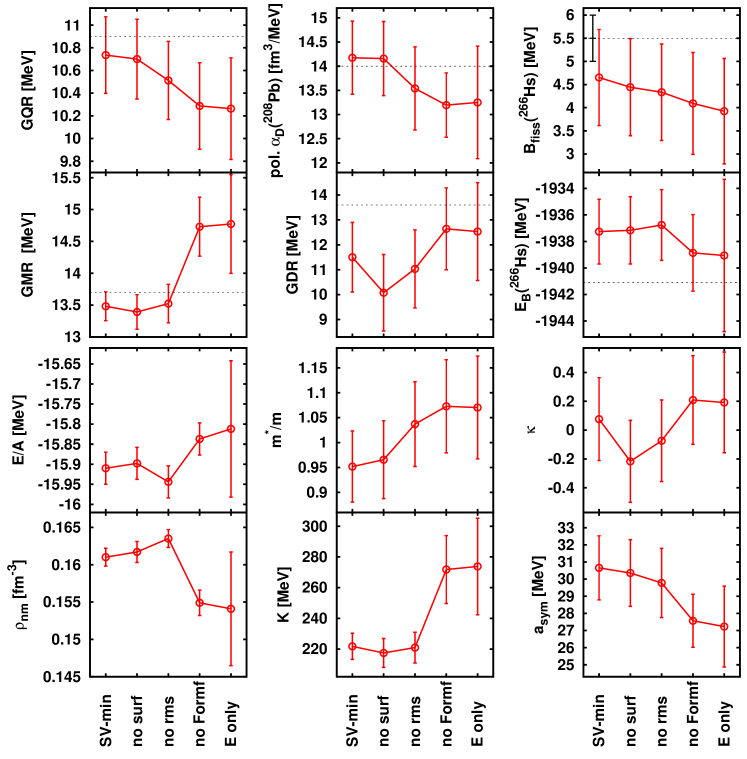
Figure 1: Lower 6 panels: Predicted nuclear-matter properties (NMP) with their extrapolation uncertainties for the parametrizations in table 1. Upper 6 panels: Predicted properties in finite nuclei, giant resonance energies and dipole polarizability $\alpha_{D}$ in ²⁰⁸Pb and binding energy $E_{B}$ as well as fission barrier $B_{f}$ in ²⁶⁶Hs. The faint dotted horizontal lines indicate the experimental data.

In this section, we look at the effect of varied fit data on predicted/extrapolated observables, nuclear matter properties (NMP) and key observables of the two nuclei ²⁰⁸Pb and ²⁶⁶Hs. In ²⁶⁶Hs, we consider the binding energy $E_{b}$ [24] and the fission barrier $B_{f}$ [25]. The experimental value for $B_{f}$ is augmented with an error bar as there remains a large uncertainty from experimental analysis. The binding energy include the rotational zero-point energy which is obligatory for deformed nuclei [23]. The fission barriers are taken relative to the collective ground state and include rotational correction [26, 27]. Note that we thus include for this observable some correlation effects beyond SHF which means that $B_{f}$ is not a pure mean-field observable. In ²⁰⁸Pb, we consider the isoscalar giant monopole (GMR) and quadrupole (GQR) resonance, the isovector giant dipole resonance (GDR), and the dipole polarizability $\alpha_{D}$. These four observables are computed with the techniques of [28]. The NMP considered are: binding energy $E/A$, density $\rho_{nm}$, incompressibility $K$, isoscalar effective mass $m^{*}/m$, symmetry energy $a_{\mathrm{sym}}$, and Thomas-Reiche-Kuhn (TRK) sum rule enhancement factor $\kappa_{\mathrm{TRK}}$, all taken at the equilibrium point of symmetric matter. Note that NMP can be viewed as observables $\hat{A}$ and equally well as model parameters $\hat{A}\equiv p_{\alpha}$. This is no principle difference. All formula for uncertainty and correlations can be employed when identifying $G^{p_{\beta}}_{\alpha}=\delta_{\alpha\beta}$. Figure 1 shows the effect of the omissions of data on the observables and their uncertainties. Changes in uncertainty indicate the impact of the omitted data group an the observable. A shift of the average shows what data are pulling in which direction.

The effects on NMP (lower six panels) are large throughout. A most pronounced shift is produced by omitting $R_{\mathrm{diffr,C}}$ (in “no Formf” and “E only”) which leads to a large jump in bulk equilibrium density $\rho_{\mathrm{nm}}$ and incompressibility $K$. There is also a jump in the isovector response $a_{\mathrm{sym}}$ in addition to the generally strong changes. It is also interesting to note that radius information keeps the effective mass $m^{*}/m$ down to values below 1 while fits without radii let $m^{*}/m$ grow visibly above one. The reason is probably that $m^{*}/m$ has an impact on the surface profile, thus on $r_{\mathrm{rms,C}}$ and $\sigma_{\mathrm{C}}$, and, in turn, also on $R_{\mathrm{diffr,C}}$. The variances, of course, grow generally when omitting data. A particularly large increase emerges for the set “E only”. This indicates that any information from the charge formfactor is extremely helpful to confine the parametrization. On the other hand, although the error bars for “E only” are generally larger than for the other parametrizations, they are still in acceptable ranges. This shows that energy data alone can already provide a reasonable parametrization.

The upper block in figure 1 shows the effect of omission of fit data on observables in finite nuclei. The three giant resonances and the polarizability $\alpha_{D}$ are known to have a one-to-one correspondence with each one NMP [7]: the GMR with $K$, the GQR with $m^{*}/m$, the GDR with $\kappa_{\mathrm{TRK}}$, and $\alpha_{D}$ with $a_{\mathrm{sym}}$. These pairs of highly correlated observables shows the same trends. Note that this one-to-one correspondence is obtained in the dedicated variation of one NMP when re-optimizing all other NMP (as explained in section 3.3); isolated variation can show more dependences as, e.g., a dependence of the GDR on $a_{\mathrm{sym}}$ [29]. Note, furthermore, that the correspondence of $\alpha_{D}$ with $a_{\mathrm{sym}}$ is equivalent to a correspondence of $\alpha_{D}$ with $\partial_{\rho}a_{\mathrm{sym}}$, because $a_{\mathrm{sym}}$ is strongly correlated with $\partial_{\rho}a_{\mathrm{sym}}$ [30]. The large effects from omission of $R_{\mathrm{diffr,C}}$ in “no Formf” which were seen in some NMP come up again here. Unlike NMP, observables in finite nuclei allow a comparison with experimental data. The giant resonances (with exception of GDR) and $\alpha_{D}$ indicate that inclusion of radius information drives into the right direction which is a gratifying feature. Inclusion of radii is also beneficial for $B_{f}(^{266}$Hs$)$ but disadvantageous for $E_{B}(^{266}$Hs$)$. It is noteworthy that the trend of $E_{B}(^{266}$Hs$)$ is similar to the trend of $\rho_{\mathrm{nm}}$. This indicates some correlation between these two observables which is seen in figure 8.

Besides the strong impact of $R_{\mathrm{diffr,C}}$, there remain only few minor effects. The set “E only” produces again a large growth of the variance for the energy observable $E_{B}(^{266}\mathrm{Hs})$ which correlates well with a similar huge growth for the bulk $E/A$.

3.1.2 Reproduction of fit observables

In this subsection, we look at the effect of varied fit data on the average and r.m.s. residuals taken over a group of data. This is a compact, although already informative, version of the study of residuals mentioned under point 5 in section 2.2. Mean values deviating significantly from zero within the scale set by the uncertainties indicate a non-statistical distribution and thus some incompatibility of the observable with the model. Changes on the r.m.s. error indicate the sensitivity to a group of observables.

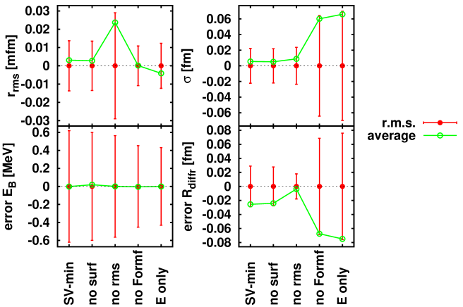
Figure 2: Average deviation (green) and r.m.s. deviation (red errorbars) for groups of observables in the pool of fit data.

Figure 2 shows the effects of the omissions on the average residuals of fit observables. The average error of energy $E_{B}$ is always near zero which is not surprising because all fits include $E_{B}$ with large weight. Note that the zero average error does not exclude missing trends which are seen when plotting the systematics of energy deviations, see e.g. [21, 7, 8].

The diffraction radius $R_{\mathrm{diffr,C}}$ is special in that it shows large average residuals for practically every case. In fact, the r.m.s. error is almost exhausted by the average error. Zero average error appears only for the set “no rms” which omits $r_{\mathrm{rms,C}}$. This indicates that there is some incompatibility between $r_{\mathrm{rms,C}}$ and $R_{\mathrm{diffr,C}}$ in the present model. Negative average error means that the $R_{\mathrm{diffr,C}}$ tend to be larger than the experimental values. The opposite trend is seen for $r_{\mathrm{rms,C}}$ (upper left panel, case “no rms”) showing that $r_{\mathrm{rms,C}}$ wants to be smaller than the data if $R_{\mathrm{diffr,C}}$ is matching perfectly. The sets “no Formf” and “E only” show where $R_{\mathrm{diffr,C}}$ ends up if it is not constrained by fit. The change of its average deviation (green lines) (and with it the average values) is significant. It grows to values of about $0.07\,\mathrm{fm}^{-3}$ which is far larger than the allowed uncertainty from SV-min of about $0.02\,\mathrm{fm}^{-3}$ (red error bars). Thus the reproduction of the charge formfactor is much degraded for these two sets. The question is whether this is an insufficiency of the SHF model or whether we see here a defect of the model for the intrinsic nucleon formfactor [6]. Note that the deviations are of the order of the adopted errors (0.04 fm^-3). This indicates that a better simultaneous adjustment of $E_{B}$ and $R_{\mathrm{diffr,C}}$ is not possible within the given SHF model. The trend of the average deviations of $R_{\mathrm{diffr,C}}$ is very similar to the trend of $\rho_{\mathrm{nm}}$ in figure 1. The correlation goes up to quantitative detail: From SV-min to “E only”, $R_{\mathrm{diffr,C}}$ grows by 0.05 fm, i.e. by about 1%. The density $\rho_{\mathrm{nm}}$ shrinks by about 0.005 fm^-3 which corresponds perfectly to the radius effect.

The surface thickness $\sigma_{\mathrm{C}}$ has generally a small average error. Omitting only $\sigma_{\mathrm{C}}$ does not change much. The correct $\sigma_{\mathrm{C}}$ emerges already if $R_{\mathrm{diffr,C}}$ is properly constrained. We see, however, a drive to smaller surfaces if all formfactor observables are omitted in the fit.

3.2 Extrapolation uncertainties

According to point 1 in section 2.2, the most obvious result of statistical analysis are the uncertainties on extrapolated observables. It is natural that extrapolations become the more risky the farther away a nucleus is from the fit pool.

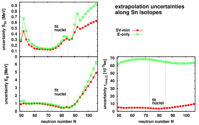
Figure 3: Extrapolation uncertainties for binding energy $E_{B}$ (lower left panel), charge r.m.s. radius $r_{\mathrm{rms,C}}$ (lower right panel), and two-neutron separation energy $S_{2n}$ (upper left panel) along the chain of even Sn isotopes. The few Sn nuclei which were included in the fits lie in between the two vertical dotted lines. Results are shown for two forces, SV-min and “E only”.

This is demonstrated in figure 3 for the chain of Sn isotopes reaching out to very neutron rich $r$-process nuclei. The uncertainties of the fit observables $E_{B}$ and $r_{rms,C}$ are smallest for the fit nuclei and grow with distance to the fit region. The growth is large, by a factor of 6–10, for the extrapolation of $E_{B}$ and of two-neutron separation energy $S_{2n}$ into the neutron-rich region. This is a direction where isovector terms become important, but isovector NMP are not so well fixed in fits to nuclear ground states. Extrapolations to superheavy elements are probing more the isoscalar channel and are thus more robust showing only factor 2–3 growth in uncertainty, see $E_{B}(^{266}\mathrm{Hs})$ in figure 1. The fit “E only” has comparable uncertainties on $E_{B}$ and $S_{2n}$ for the fit nuclei, but shows slightly faster growth outside this region. The effect is not dramatic which indicates that fits to energy suffice to predict energy observables. Different is the observable $r_{rms,C}$. The fit “E only” has an order of magnitude larger uncertainties than SV-min. However, both forces agree in the trend which is very flat over the whole chain. Predictions for radii thus are robust once radii are well fitted.

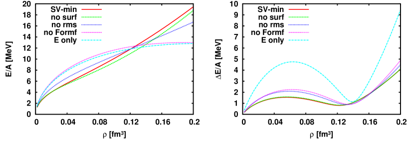
Figure 4: Left: $E/A$ versus density for pure neutron matter for the parametrization developed with the fit protocol of SV-min while omitting certain blocks of observables. Right: The extrapolation uncertainties for the data shown in the left panel.

A very far extrapolation is involved in studying pure neutron matter as it is often done in nuclear astrophysics (see [31, 18, 32] and citations therein). The left panel of figure 4 shows the equation of state (EoS) $E/A_{\mathrm{neut}}(\rho)$ for pure neutron matter. There arise huge differences in its slope at $\rho<0.12\,\mathrm{fm}^{-3}$ and $\rho>0.15\,\mathrm{fm}^{-3}$. In spite of these very different slopes, all EoS share about the same values around neutron density $\rho\approx{0.13}$ fm^-3. It looks like a “fixpoint” in the neutron EoS.

The right panel shows the corresponding extrapolation uncertainties. The errors follow the same trends as the deviations between the parametrizations in the left panel. In regions of large deviations, these are larger than the estimated uncertainties. The discrepancy indicates that systematic errors will play a role here. What the $\rho$-dependence of the uncertainties is concerned, it is astonishing that there arises a pronounced minimum just near this “magic” density $\rho\approx{0.13}$ fm^-3 where all predictions approximately agree. Although, the actual position of the minimum varies a bit with the force the coincidence looks impressive. The reasons for this particularly robust point has yet to be found out.

The difference in neutron EoS, and particularly the difference in slope for $\rho<0.12\,\mathrm{fm}^{-3}$, has dramatic consequences for the stability of neutron stars. The two forces with small slope “no Formf” and “E only” do not yield a maximal radius at all because the neutron EoS becomes unbound for very large densities.

3.3 Variation of nuclear matter properties (NMP)

We now come to point 4 of section 2.2, the dedicated variation of model parameters. We do that in terms of the NMP which are a form of model parameters with an intuitive physical content. We consider here a variation of only one NMP at a time (this differs from the variation in [7] where four NMP were kept fixed). Thus we keep only the one varied NMP at a dedicated value and fit all remaining, now 13, model parameters. This is so to say a correlated variation because it allows the other model parameters to find their new optimum value for the one given constrained NMP.

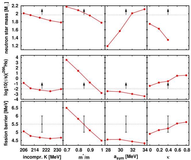
Figure 5: Results from systematic variation of NMP. The maximal mass of neutron stars (upper), fission lifetime (middle) and fission barrier (lower) in ²⁶⁶Hs as function of the four varied NMP ($K$, $m^{*}/m$, $a_{\mathrm{sym}}$, or $\kappa_{\mathrm{TRK}}$). One NMP was fixed while performing free fit of all other parameters. In cases where data is missing for the neutron star mass, the equation of state is not stable for high densities (see figure 4). Dashed lines show experimental data for the maximal neutron star mass [33], the lifetime [34] and the barrier [25] of ²⁶⁶Hs. Up-arrows indicate that these data are just lower limits.

Figure 5 shows the maximal neutron star mass obtained by solving the Tolman-Oppenheimer-Volkoff equation (see [32] for details) as well as fission barriers and fission lifetimes of the super-heavy nucleus ²⁶⁶Hs. Fission barriers were determined with respect to the collective ground state energy. The collective ground state and the lifetime were calculated using the procedure as described in [27]. The incompressibility $K$ has little effect on all three observables while the effective mass $m^{*}/m$ shows always strong trends. The effect on ²⁶⁶Hs is understandable because $m^{*}/m$ determines the spectral density and with it the shell-corrections which are known to have a strong influence on the fission path. Different behaviors are seen for $a_{\mathrm{sym}}$ and $\kappa_{\mathrm{TRK}}$. Neutron matter depends sensitively on these isovector parameters while fission in ²⁶⁶Hs reacts less dramatic, although there remains a non-negligible trend also here. However strong or weak the trends, all three observables gather influences from several NMP. Unlike the case of giant resonances [7], there is here no one-to-one correspondence between an observable and one NMP.

3.4 Covariances

Statistical correlations, also called covariances ${c}_{AB}$ between two observables $A$ and $B$, see point 2 of section 2.2, are a powerful tool to explore the hidden connections within a model. This quantity helps, e.g., to determine the information content of a new observable added to an existing pool of measurements. Examples and detailed discussions are found in previous papers [35, 11, 13]. We add here two new cases related to the observables and parametrizations addressed in this paper.

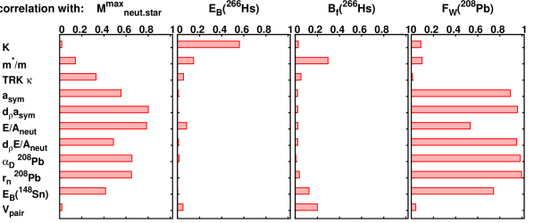
Figure 6: Correlations of the maximal mass of a neutron star, of the binding energy and of the fission barrier of the isotope ²⁶⁶Hs, and of the weak-charge formfactor $F_{W}(q\!=\!0.475/\mathrm{fm})$ in ²⁰⁸Pb with NMP and a couple of observables in finite nuclei, for the force SV-min. The $E/A_{\mathrm{neut}}$ stands for the neutron EoS at $\rho=0.1$ fm^-3 and $d_{\rho}E/A_{\mathrm{neut}}$ for its slope at this density. $\alpha_{D}$ is the dipole polarizability, and $r_{\mathrm{n}}$ the neutron r.m.s. radius. For the pairing strength, we show only the proton case. The correlations for neutron pairing strength are equivalent.

Figure 6 shows the covariances for four observables, three of them being far extrapolations and one rather at the safe side. The latter case is the weak-charge formfactor $F_{W}$ in ²⁰⁸Pb (right panel), taken at momentum $q\!=\!0.475/\mathrm{fm}$, which is known to be closely related to the neutron radius [12]. It is fully correlated with all the static isovector observables $a_{\mathrm{sym}}$, $d_{\rho}E/A_{\mathrm{neut}}$, and $\alpha_{D}$, but uncorrelated with the isoscalar NMP and the dynamic isovector response $\kappa_{\mathrm{TRK}}$. As an example for an exotic nucleus deep in the astro-physical $r$-process region, we have included ¹⁴⁸Sn in the considerations. The strong isovector correlations provide also a sizable correlation with this extremely neutron rich ¹⁴⁸Sn.

The maximal mass of a neutron star (left panel) shows a somewhat more mixed picture. It is, not surprisingly, most strongly correlated with the neutron EoS. There are also sizable correlations with all the static isovector observables (block from $a_{\mathrm{sym}}$ to $r_{n}$) and to some extend with the extrapolation to the extremely neutron rich ¹⁴⁸Sn as well as $\kappa_{\mathrm{TRK}}$. Very little correlation exists with the isoscalar NMP $K$ and $m^{*}/m$.

A much different picture emerges for the binding energy of the super-heavy ²⁶⁶Hs: There is no really large correlation with any observable shown here. Negligible are correlations with static isovector observables. Some correlations exit for the parameters $K$, $m^{*}/m$, $\kappa_{\mathrm{TRK}}$, and $V_{\mathrm{pair}}$ which indicates that all these four parameters have some impact on $E_{B}(^{266}$Hs$)$. The fission barrier $B_{f}(^{266}\mathrm{Hs})$ shows similarly a collection of many small correlations. The most pronounced here is the correlation with the effective mass $m^{*}/m$. This agrees with results in figure 5, where only $m^{*}/m$ shows a significant trend for $B_{f}$. Next to $m^{*}/m$ comes the influence from pairing strength which is not surprising as pairing has a large effect near the barrier where the density of states is high.

We have seen in figure 4 that the neutron EoS has a pronounced variation of extrapolation uncertainties as function of $\rho$. In particular, there is a marked minimum at $\rho\approx$ 0.13 fm^-3.

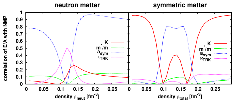
Figure 7: Correlations of $E/A$ at various densities with the basic nuclear matter parameters (NMP). Left: for the neutron $E/A_{\mathrm{neut}}$. Right: for $E/A_{\mathrm{sym}}$ of symmetric nuclear matter.

As complementing information, we show in the left panel of figure 7 the correlation of $E/A_{\mathrm{neut}}(\rho)$ for neutron matter with the basic NMP. Not surprisingly, the symmetry energy $a_{\mathrm{sym}}$ dominates, at least in the regions of low and high density. We see a minimum of correlations for all NMP, except $\kappa_{\mathrm{TRK}}$, just in the region where uncertainties are lowest and where all predictions for $E/A_{\mathrm{neut}}$ agree, see figure 4. This is a remarkable coincidence for which we have not yet an explanation.

The right panel of figure 7 shows the correlations for $E/A$ of symmetric matter (right panel), $K$ is strongly correlated and dominates at low and high densities. It is interesting to see that $a_{\mathrm{sym}}$ dominates with sizable correlations in the region $\rho=$0.10–0.16 fm^-3. This is plausible because these are the typical density values in the inner surface of a nucleus and this is the region where the dipole response is predominantly explored. The dynamic NMP, $m^{*}/m$ and $\kappa_{\mathrm{TRK}}$, are almost uncorrelated everywhere.

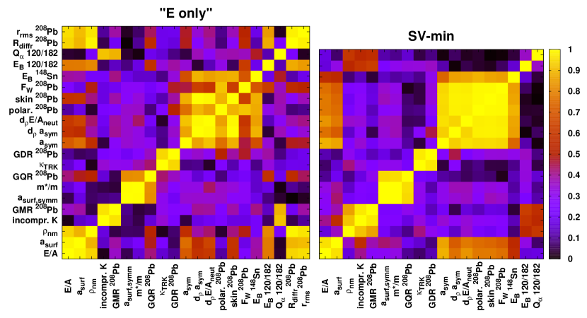
Figure 8: Correlation matrix for a couple of observables computed from the fit to all data SV-min (right panel) and “E only” where all information from radii and surface thickness is omitted (left panel). High correlation is indicated by light yellow, no correlation by deep black.

Figure 8 shows the matrix of pairwise covariances for a selection of NMP and observables in finite nuclei. A matrix for SV-min (right panel) was already discussed in [20]. It segregates nicely into four groups of observables: static isoscalar around $K$, dynamic isoscalar around $m^{*}/m$, static isovector around $a_{\mathrm{sym}}$, and dynamic isovector around $\kappa_{\mathrm{TRK}}$. The basic bulk NMP $E/A$ and $\rho_{\mathrm{nm}}$ are weakly correlated with the static isovector block. The same block is also weakly correlated with the extremely neutron rich extrapolation ¹⁴⁸Sn. The far superheavy nucleus Z=120/N=182 has a bit of low correlations to all other observables, similar to ²⁶⁶Hs in figure 6.

The left panel of figure 8 shows the result for the set “E only”. The four blocks of mutually correlated observables remain almost the same, however, sometimes with somewhat reduced correlation. A marked change appears for $\rho_{\mathrm{nm}}$ which was strongly linked to the static isoscalar $K$ block for SV-min and now moves totally to the basic NMP $E/A$. This case demonstrates that changing the fit data can have an impact on the covariances, and in general does. It is rather surprising that the two fits show so widely similar trends in covariances.

The set “E only” does not include any radius information in the data. This allows to compute also the covariances with charge radii. The left panel thus includes also $R_{\mathrm{diffr,C}}$ and $r_{\mathrm{rms,C}}$ amongst the observables. Both, $R_{\mathrm{diffr,C}}$ and $r_{\mathrm{rms,C}}$, have about the same correlations. These are strong with the block of basic NMP $E/A$ and $\rho_{\mathrm{nm}}$ plus the isoscalar surface energy $a_{\mathrm{surf}}$. This confirms the findings from figure 1 where we see that radius information has a large impact on the basic bulk binding. There are some correlations with the binding energy of the superheavy element Z=120/N=182 which is not a surprise as this nucleus also correlates with the block $E/A$ and $\rho_{\mathrm{nm}}$. All other correlations are not significant.

3.5 Beyond linear analysis

Standard $\chi^{2}$-analysis assumes that an observable $A(\mathbf{p})$ depends linearly on the model parameters $\mathbf{p}$ within the range of reasonable $\mathbf{p}$. We have checked that assumption by carrying the expansion (6) for the observables up to quadratic terms still assuming a quadratic form for $\chi^{2}$ as function of the parameters. The simple rules of integrating polynomials with Gaussians allow to compute uncertainties and correlations also for this non-liner case in straightforward manner.

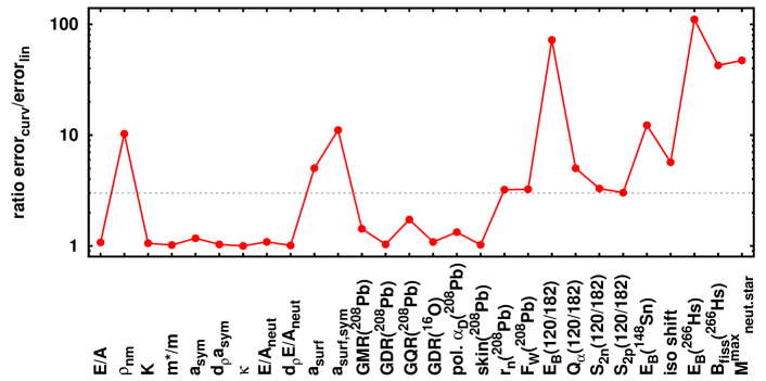
Figure 9: Ratio of extrapolation uncertainties with curvature correction and without computed with SV-min. The horizontal line indicates a critical ratio of 3 above which curvature effects become important.

Figure 9 shows the ratio of extrapolation uncertainties computed from the quadratic expansion to those from the linear model for a broad selection of observables. We had also checked the weight of the quadratic terms explicitly and this delivers the same picture. Thus we take this ratio as a simple measure of (non-)linearity. The faint black horizontal line indicates the limit up to which the assumption of linearity is acceptable. Most observables are thus in the linear regime, a few of them reach into the non-linear regime, and some of them (superheavy elements and neutron stars) are dramatically non-linear with ratios going up to 100. However, this example has to be taken as an order of magnitude estimate. Such a highly non-linear requires a more careful evaluation of correlation according to Spearman’s analysis [36] which goes beyond the scope of this paper.

We have also checked the effect of non-linearity on covariances $c_{AB}$ for SV-min. The basic sorting into strongly correlated combinations and weakly correlated ones is maintained. It is only at closer inspection that one can spot some changes of correlations if a non-linear observable is involved. In most cases, non-linearity’s reduce correlations slightly.

4 Conclusions and outlook

We have explored the uncertainties inherent in the Skyrme-Hartree-Fock (SHF) approach by employing, out of many, five different strategies for error estimates: extrapolation error from $\chi^{2}$ analysis, covariances between pairs of observables from $\chi^{2}$ analysis, trends with systematically varied model parameters (practically nuclear matter parameters), trends of residual errors, and block-wise variation of fit data. For the latter strategy, we have fitted a couple of new parametrizations where differing groups of fit observables had been omitted, once the r.m.s. radii, once the surface thickness, once both formfactor observables (surface, diffraction radius), and finally all form information (surface, diffraction radius, r.m.s. radius). This makes, together with the full fit, five parametrizations which are then used in combination with all further analysis. Some of the strategies yield similar information (e.g. trend with parameters and covariances), however from different perspectives which makes it useful to consider both. In any case, the combination of strategies is more informative than any single strategy alone. Out of the many interesting aspects worked out in the above studies, we emphasize here a few prominent findings and indicate the directions for further development:

1. Fits only to binding energy (omitting any radius information) yield already a very acceptable description of nuclear properties. The error on diffraction radius and surface thickness grows by factor 3–4, but remains with about 0.08 fm in an acceptable range. However, the uncertainties in extrapolations can grow large which proves the usefulness of having radius information in the fit. Radius information is strongly correlated with bulk binding (equilibrium energy and density) as well as surface energy and it helps to fix theses quantities.

2. We have found a conflict between the description of r.m.s. radius and diffraction radius. Fitting only one of the both spoils the other one. Fitting both yields a compromise. The precision which can be achieved is small (0.02–0.04 fm), but limited to that in the present model. Further development work on SHF and the computation of radii is required to harmonize the data.

3. Extrapolations to exotic nuclei show, of course, increasing uncertainties with increasing distance to the set of fit nuclei. The growth of errors is large for energies of $r$-process nuclei (factor 6–10) and moderate for energies of super-heavy elements (factor 2–3). Errors on radii, on the other hand, remain even nearly constant. This is related to the tight connection of radii to bulk binding (see point 1 above).

4. The more dramatic extrapolation to neutron stars is plagued by much larger uncertainty. Neutron matter is highly correlated to isovector forces which are less well fixed by fits to existing nuclei. The variation of fit data shows that there are probably large systematic errors beyond the statistical uncertainties. In spite of the generally large uncertainties, there is a “magic” region around density 0.13 fm^-3 where all parametrizations yield surprisingly small uncertainties and very similar predictions. This effect deserves further investigation.

5. We have checked the assumption of linear parameter dependence, employed in standard statistical analysis, for many observables. Most of them show sufficient linearity, but some deviate dramatically. These are typically the observables in far extrapolations, exotic nuclei and neutron stars. The impact of non-linearity on extrapolation uncertainties and covariances has yet to be investigated.

Acknowledgments: This work was supported by the Bundesministerium für Bildung und Forschung (BMBF) under contract number 05P09RFFTB.

References

References

- [1] Negele J W and Vautherin D 1972 Phys. Rev. C 5 1472
- [2] Reinhard P G and Toepffer C 1994 Int. J. Mod. Phys. E 3 435
- [3] Beiner M, Flocard H, Nguyen Van Giai and Quentin P 1975 Nucl. Phys. A238 29–69
- [4] Bartel J, Quentin P, Brack M, Guet C and Håkansson H B 1982 Nucl. Phys. A386 79–100
- [5] Tondeur F, Brack M, Farine M and Pearson J 1984 Nucl. Phys. A 420 297
- [6] Friedrich J and Reinhard P G 1986 Phys. Rev. C 33 335–351
- [7] Klüpfel P, Reinhard P G, Bürvenich T J and Maruhn J A 2009 Phys. Rev. C 79 034310
- [8] Kortelainen M, Lesinski T, Moré J, Nazarewicz W, Sarich J, Schunck N, Stoitsov M V and Wild S 2010 Phys. Rev. C 82 024313
- [9] Piekarewicz J, Agrawal B K, Colò G, Nazarewicz W, Paar N, Reinhard P G, Roca-Maza X and Vretenar D 2012 Phys. Rev. C 85 041302
- [10] Nazarewicz W, Reinhard P G, Satuła W and Vretenar D 2013 Eur. Phys. J. A; arXiv:1307.5782
- [11] Reinhard P G and Nazarewicz W 2013 Phys. Rev. C 87 014324
- [12] Reinhard P G, Piekarewicz J, Nazarewicz W, Agrawal B K, Paar N and Roca-Maza X 2013 Phys. Rev. C 88 034325
- [13] Dobaczewski J, Nazarewicz W and Reinhard P G 2014 J. Phys. G 41
- [14] Bender M, Heenen P H and Reinhard P G 2003 Rev. Mod. Phys. 75 121
- [15] Brandt S 1997 Statistical and computational methods in data analysis (Springer, New York)
- [16] Bevington P R and Robinson D K 2003 Data Reduction and Error Analysis for the Physical Sciences (McGraw-Hill)
- [17] Tarantola A 2005 Inverse problem theory and methods for model parameter estimation (SIAM, Philadelphia)
- [18] Stone J and Reinhard P G 2007 Prog. Part. Nucl. Phys. 58 587
- [19] Erler J, Klüpfel P and Reinhard P G 2011 J. Phys. G 38 033101
- [20] Kortelainen M, McDonnell J, Nazarewicz W, Reinhard P G, Sarich J, Schunck N, Stoitsov M V and Wild S M 2012 Phys. Rev. C 85 024304
- [21] Erler J, Klüpfel P and Reinhard P G 2010 J. Phys. G 37 064001
- [22] Friedrich J and Vögler N 1982 Nucl. Phys. A 373 192
- [23] Klüpfel P, Erler J, Reinhard P G and Maruhn J A 2008 Eur. Phys. J A 37 343
- [24] Wang M, Audi G, Wapstra A, Kondev F, MacCormick M, Xu X and Pfeiffer B 2012 Chinese Physics C 36 1603
- [25] Péter J 2004 Eur. Phys. J. A 22 271
- [26] Schindzielorz N, Erler J, Klüpfel P, Reinhard P G and Hager G 2009 Int. J. Mod. Phys. E 18 773
- [27] Erler J, Langanke K, Loens H P, Martinez-Pinedo G and Reinhard P G 2012 Phys. Rev. C 85 025802
- [28] Reinhard P G 1992 Ann. Phys. (Leipzig) 504 632
- [29] Trippa L, Colò G and Vigezzi E 2008 Phys. Rev. C 77 061304
- [30] Roca-Maza X, Brenna M, Col‘o G, Centelles M, ̵̃nas X V, Agrawal B K, Paar N, Vretenar D and Piekarewicz J 2013 Phys. Rev. C 88 024316
- [31] Lattimer J M 2012 Ann. Rev. Nucl. Part. Sci. 62 485
- [32] Erler J, Horowitz C J, Nazarewicz W, Rafalski M and Reinhard P G 2013 Phys. Rev. C 87 044320
- [33] Demorest P B, Pennucci T, Ransom S M, Roberts M S E and Hessels J W T 2010 Nature 467 209
- [34] Hofmann S, Heßberger F, Ackermann D, Antalic S, Cagarda P, Fwiok S, Kindler B, Kojouharova J, Lommel B, Mann R, Münzenberg G, Popeko A, Saro S, Schött H and Yeremin A 2001 Eur. Phys. J. A 10(1) 5–10
- [35] Reinhard P G and Nazarewicz W 2010 Phys. Rev. C 81 051303
- [36] Schmid F and Schmidt R 2007 Statistics and probability letters 77 407