The Not-So-Sterile 4th Neutrino:
Constraints on New Gauge Interactions from Neutrino Oscillation Experiments

Abstract

Sterile neutrino models with new gauge interactions in the sterile sector are phenomenologically interesting since they can lead to novel effects in neutrino oscillation experiments, in cosmology and in dark matter detectors, possibly even explaining some of the observed anomalies in these experiments. Here, we use data from neutrino oscillation experiments, in particular from MiniBooNE, MINOS and solar neutrino experiments, to constrain such models. We focus in particular on the case where the sterile sector gauge boson $A^{\prime}$ couples also to Standard Model particles (for instance to the baryon number current) and thus induces a large Mikheyev-Smirnov-Wolfenstein potential. For eV-scale sterile neutrinos, we obtain strong constraints especially from MINOS, which restricts the strength of the new interaction to be less than $\sim 10$ times that of the Standard Model weak interaction unless active–sterile neutrino mixing is very small ($\sin^{2}\theta_{24}\lesssim 10^{-3}$). This rules out gauge forces large enough to affect short-baseline experiments like MiniBooNE and it imposes nontrivial constraints on signals from sterile neutrino scattering in dark matter experiments.

I Introduction and motivation

The possible existence of sterile neutrinos (Standard Model singlet fermions) with masses of order eV has been a widely discussed topic in astroparticle physics over the past few years. It is motivated by several anomalous results from short-baseline neutrino oscillation experiments, in particular the excesses of $\nu_{e}$ and $\bar{\nu}_{e}$ events in a $\nu_{\mu}$ and $\bar{\nu}_{\mu}$ beam respectively observed by LSND [1] and MiniBooNE [2], the apparently lower than expected $\bar{\nu}_{e}$ flux from nuclear reactors [3, 4, 5] (see however [6]) and the deficit of $\nu_{e}$ in radioactive source experiments [7, 8]. Global fits [9, 10, 11, 12, 13, 14, 11, 15] show that these anomalies could be explained if sterile neutrinos with $\mathcal{O}(\text{eV})$ mass and $\mathcal{O}(10\%)$ mixing with $\nu_{e}$ and $\nu_{\mu}$ exist. However, global fits also reveal that it is difficult to reconcile such a scenario with existing null results from other short-baseline oscillation experiments.

Constraints come also from cosmological observations, which slightly disfavor scenarios with extra relativistic degrees of freedom in the early Universe [16]. Cosmology also imposes a tight constraint on the sum of neutrino masses $\sum_{j}m_{\nu j}<0.23$, where the sum runs over all neutrino mass eigenstates that are in thermal equilibrium in the early Universe. Note that these constraints would be relaxed if the recent BICEP-2 data on B-modes in the cosmic microwave background [17] is confirmed [18, 19, 20, 21, 22].

An interesting scenario that is unconstrained by cosmology is self-interacting sterile neutrinos [23, 24]. If interactions among sterile neutrinos are mediated by a scalar or gauge boson with a mass of order MeV or lighter, sterile neutrinos will feel a strong thermal potential in the early Universe which suppresses their mixing with active neutrinos and thus prohibits their production through oscillations. Moreover, if the new interaction couples not only to sterile neutrinos, but also to dark matter, it has the potential to explain several problems with cosmic structure formation at small scales [24, 25].

If a new interaction is shared between sterile neutrinos and ordinary matter (for instance in models with gauged baryon number coupled to sterile neutrinos and in scenarios in which a sterile sector gauge boson mixes kinetically with the photon), interesting signals in direct dark matter searches are possible [26, 27, 28, 29]. The increased neutrino–nucleus scattering cross section might even explain some of the excess events observed by several experiments. On the other hand, such scenarios are more challenging for cosmology because of an additional sterile neutrino production mechanism through the gauge interaction. (Note that these constraints are still avoided for instance in scenarios with extra entropy production in the visible sector after sterile neutrino decoupling [30].)

In this paper, we investigate how novel interactions between sterile neutrinos and ordinary matter are constrained by neutrino oscillation experiments at short and long baseline. This topic has been discussed in a previous paper [31], the conclusions of which we will update below. For definiteness, we will focus on scenarios similar to the “baryonic sterile neutrino” scenario first introduced in [26], where the sterile neutrino couples to gauged baryon number. We emphasize, however, that our results are directly applicable to any theory in which sterile neutrinos interact with Standard Model (SM) fermions through a new gauge force under which ordinary matter carries a net charge. (The last condition excludes models in which the coupling is only through kinetic mixing between the new gauge boson and the photon.) The new gauge current creates a Mikheyev-Smirnov-Wolfenstein (MSW) potential for sterile neutrinos propagating through ordinary matter and has thus a potentially large impact on neutrino oscillations. Since the mass of the new gauge boson in this model can be as low as 10 MeV (see [27] for detailed constraints) and since constraints on its coupling are weak [26], the strength of the effective interaction can be more than two orders of magnitude larger than the SM weak interactions responsible for the ordinary MSW effect. This implies that resonant enhancement of the oscillation amplitude could be relevant at $\mathcal{O}(\text{GeV})$ energies even for relatively large mass squared difference $\Delta m_{41}^{2}\sim\text{eV}$ between the mostly sterile and mostly active mass eigenstates. The model could thus potentially allow an explanation of some of the short-baseline oscillation anomalies with significantly smaller vacuum mixing angles than in sterile neutrino scenarios without new interactions.

The structure of the paper is as follows. In section II, we briefly review models with new interactions in the sterile sector in general, and the “baryonic neutrino” model from [26] in particular. We map these models onto an effective field theory and discuss their implications for neutrino oscillations. In particular, we derive approximate analytical formulas for the oscillation probabilities. In section III, we then present our main numerical results, which will set strong constraints on new forces coupling sterile neutrinos to SM particles. We will summarize and conclude in section IV.

II Models and formalism

II.1 New gauge bosons in the sterile neutrino sector

In the following we shortly describe the model proposed in [26, 27], originally introduced to study the impact of a new gauge force in the sterile neutrino sector on dark matter searches. The basic idea is to introduce a fourth left-handed neutrino flavour $\nu_{b}$, sterile under SM interactions, which can have a relatively large coupling to baryons ($10^{2}$–$10^{3}$ times larger than the Fermi constant $G_{F}$) without being in conflict with current experimental bounds, like for examples constraints coming from meson decays such as $K\rightarrow\pi\bar{\nu}_{b}\nu_{b}$ [26]. It can be implemented by introducing a new $U(1)_{B}$ gauge symmetry under which quarks have charge $g_{b}/3$ and the baryonic neutrino $\nu_{b}$ has charge $g_{b}^{\prime}$. We will assume $g_{b}$ and $g_{b}^{\prime}$ to be of order 0.1–1. To cancel anomalies, the introduction of additional fermions charged under $U(1)_{B}$ will be necessary, but we assume that these do not mix significantly with SM neutrinos and can be neglected. The baryonic gauge boson $X$ acquires a mass when $U(1)_{B}$ is broken by a new sterile sector Higgs field $h_{b}$. The relevant part of the Lagrangian after symmetry breaking can be written as [26]

$$\operatorname{\mathcal{L}} \supset -\frac{1}{4}F_{X,\mu\nu}F_{X}^{\mu\nu}+\frac{1}{2}m_{X}^{2}X_{\mu}X^{\mu}$$ (1)

$$+\bar{\nu}_{b}\gamma_{\mu}\big{(}i\partial^{\mu}+g_{b}^{\prime}X^{\mu}\big{)}\nu_{b}+\sum_{q}\bar{q}\Big{(}i\not{D}_{\text{SM}}+\frac{1}{3}g_{b}\gamma_{\mu}X^{\mu}\Big{)}q+\operatorname{\mathcal{L}}_{m}\text{,}$$

where $q$ are the SM quark fields, $F_{X,\mu\nu}\equiv\partial_{\mu}X_{\nu}-\partial_{\nu}X_{\mu}$ is the field strength tensor of the baryonic vector boson $X_{\mu}$ and $m_{X}\sim 1\,\text{GeV}$ is its mass. In a seesaw framework, the baryonic neutrino mixes with the SM through the terms

$$\operatorname{\mathcal{L}}_{m}=-\sum_{\alpha,j}m_{D}^{\alpha j}\bar{\nu}_{L}^{\alpha}N_{R}^{j}-\sum_{j}m_{b}^{j}\bar{\nu}_{bL}N_{R}^{j}-\frac{1}{2}\sum_{i\text{,}j}m_{R}^{ij}\overline{\left(N_{R}^{i}\right)^{C}}N_{R}^{j}+h.c.\,,$$ (2)

with the Dirac mass matrix $m_{D}$ of the active neutrinos $\nu_{L}^{\alpha}$, the Dirac mass vector of the baryonic neutrino $m_{b}^{j}$ and the the Majorana mass matrix $m_{R}^{ij}$ of the heavy right-handed neutrino fields $N_{R}^{j}$. The flavour index $\alpha$ runs over $e$, $\mu$ and $\tau$, while the indices $i$ and $j$ run over all heavy right-handed neutrino states.

The Lagrangian of equation (1) implies the existence of a new MSW potential that sterile neutrinos experience while propagating in matter. This effect is caused by coherent elastic forward scattering on neutrons and protons and can lead to resonant enhancement of flavour oscillations. Since coherent forward scattering does not involve any momentum transfer, its amplitude can be most easily obtained from the low energy effective Lagrangian of baryonic neutral current interactions

$$\operatorname{\mathcal{L}}_{b,\text{eff}} = \frac{G_{B}}{2}\big{[}\bar{\nu}_{b}\gamma_{\mu}\left(1-\gamma_{5}\right)\nu_{b}\big{]}\big{[}\bar{p}\gamma^{\mu}p+\bar{n}\gamma^{\mu}n\big{]}\text{.}$$ (3)

Here, the effective coupling constant is $G_{B}\equiv g_{b}g_{b}^{\prime}/m_{X}^{2}$. By treating neutrons and protons as a static background field [32], we obtain the matter potential for sterile neutrinos

$$V_{b}=G_{B}N_{\text{nucl}}\text{.}$$ (4)

The potential for sterile anti-neutrinos has opposite sign. Here, $N_{\text{nucl}}$ is the number density of nucleons in the background matter. Note that $G_{B}$ can be either positive or negative, depending on the relative sign of $g_{b}$ and $g_{b}^{\prime}$. In the following analysis we will use the ratio of the coupling constants

$$\epsilon\equiv\frac{G_{B}}{\sqrt{2}G_{F}}$$ (5)

as a measure for the relative strength of $V_{b}$ compared to the potential $V_{\text{CC}}$ that charged current (CC) interactions with electrons induce for electron neutrinos in the SM. The baryonic potential can be written as

$$V_{b} =V_{\text{CC}}\cdot G_{B}/(\sqrt{2}G_{F}Y_{e})=\epsilon\,V_{\text{CC}}/Y_{e}$$ (6)

$$=\epsilon\cdot 7.56\cdot 10^{-14}\ \text{eV}\cdot\bigg{(}\frac{\rho}{\text{g}/\text{cm}^{3}}\bigg{)},$$ (7)

where $Y_{e}$ is the number of electrons per nucleon.

As mentioned in the introduction, baryonic sterile neutrinos could lead to novel signals in direct dark matter searches thanks to an enhanced sterile neutrino–nucleus scattering rate. Typically, observable effects in current experiments are expected if $\epsilon\gtrsim 100$ [26, 27, 28, 29]. We will see in section III.2 that such large values of $\epsilon$ are largely excluded for eV scale sterile neutrinos with substantial mixing into the active sector.

We wish to stress here that, while we use baryonic sterile neutrinos as a benchmark scenario, our results will apply to any scenario in which sterile neutrinos have new gauge interactions with SM fermions. It is important to keep in mind, though, that models with new forces in the lepton sector are much more tightly constrained than new baryonic interactions (see e.g. [27] for a review).

The mass terms in equation (2) lead to flavour mixing between $\nu_{b}$ and the active neutrinos, as can be seen by integrating out the heavy right-handed neutrinos and diagonalizing the resulting mass matrix. In this way, we obtain the $4\times 4$ mixing matrix $U$ connecting mass eigenstates $|\nu_{i}\rangle$ and flavour eigenstates $|\nu_{\alpha}\rangle$:

$$|\nu_{\alpha}\rangle=\sum_{i}U_{\alpha i}^{*}|\nu_{i}\rangle\text{.}$$ (8)

Since $U$ is unitary, it can be parametrized by $6$ rotation angles $\theta_{ij}$ and $3$ complex phases $\delta_{ij}$ 

$$U = R_{34}\cdot R_{24}^{\prime}\cdot R_{14}^{\prime}\cdot R_{23}\cdot R_{13}^{\prime}\cdot R_{12}\text{.}$$ (9)

Here, $R_{ij}$ describes a rotation matrix in the $ij$ plane, while $R_{ij}^{\prime}$ corresponds to a complex rotation by the angle $\theta_{ij}$ and phase $\delta_{ij}$. Given the mixing matrix $U$ and the mass squared difference $\Delta m^{2}_{41}$ between the mostly sterile mass eigenstate $\nu_{4}$ and the mostly active mass eigenstate $\nu_{1}$, one can write down the effective Hamiltonian in flavour space:

$$H^{\text{flavour}}_{\text{eff}}=\frac{1}{2E}U\begin{pmatrix}0&&&\\ &\Delta m_{21}^{2}&&\\ &&\Delta m_{31}^{2}&\\ &&&\Delta m_{41}^{2}\end{pmatrix}U^{{\dagger}}+\begin{pmatrix}V_{\text{CC}}&&&\\ &0&&\\ &&0&\\ &&&V_{b}-V_{NC}\end{pmatrix}\text{.}$$ (10)

Here, $V_{NC}\equiv-\sqrt{2}G_{F}n_{n}/2$ is the contribution from SM neutral current interactions to the MSW potential. It is proportional to the number density $n_{n}$ of neutrons in the background material.

The oscillation probability $P_{\nu_{\alpha}\rightarrow\nu_{\beta}}(t)$, i.e. the probability for a neutrino of initial flavour $\alpha$ to be converted into flavour $\beta$ after traveling a time $t$, can then be obtained by diagonalizing the effective Hamiltonian according to $H^{\text{flavour}}_{\text{eff}}=\tilde{U}\text{diag}(\lambda_{1},\lambda_{2},\lambda_{3},\lambda_{4})\tilde{U}^{{\dagger}}$ and inserting the eigenvalues $\lambda_{i}$ and the effective mixing matrix $\tilde{U}$ into the well-known formula

$$P_{\nu_{\alpha}\rightarrow\nu_{\beta}}=\big{|}\left\langle\nu_{\beta}|\nu_{\alpha}(t)\right\rangle\big{|}^{2}=\Big{|}\sum_{j}{\tilde{U}_{\alpha j}}^{*}\tilde{U}_{\beta j}e^{-i\lambda_{j}L}\Big{|}^{2}\text{.}$$ (11)

II.2 Approximate oscillation probabilities

As a prelude to the numerical fits we are going to present in section III, we give here approximate analytic expressions for the oscillation probabilities in the baryonic sterile neutrino model and in models with new sterile neutrino–SM interactions in general. Similar calculations have been carried out previously in [31] and we will compare these results to ours in section II.3.

Our starting point is to assume $\lvert\Delta m_{41}^{2}\rvert\gg\lvert\Delta m_{31}^{2}\rvert,\Delta m_{21}^{2}$, which is a good approximation at sufficiently short baselines. Moreover, we neglect the SM MSW potentials $V_{\text{NC}}$ (arising from $Z$ exchange diagrams) and $V_{\text{CC}}$ (arising from $W$ exchange diagrams) against the baryonic potential $V_{b}$, which we assume to be much larger. With these approximations, mixing among the three active flavour eigenstates becomes irrelevant. (They can, however, still oscillate into each other through their mixing with $\nu_{b}$.) We also set $U_{\tau 4}=0$ for simplicity, following [31]. With these assumptions, diagonalization of the Hamiltonian $H^{\text{flavour}}_{\text{eff}}$ from equation (10) yields for the eigenvalues $\lambda_{i}$

$$\lambda_{1}=\lambda_{2}=0\text{,}\qquad\lambda_{3}=\frac{1}{2}\Big{(}V_{b}+\frac{\Delta m_{41}^{2}}{2E}-A\Big{)}\text{,}\qquad\lambda_{4}=\frac{1}{2}\Big{(}V_{b}+\frac{\Delta m_{41}^{2}}{2E}+A\Big{)}\text{.}$$ (12)

The elements of the unitary matrix $\tilde{U}$ are

$$\tilde{U}_{\mu 1}=\tilde{U}_{e1}=0\text{,}\qquad\lvert\tilde{U}_{e2}\rvert^{2}=\frac{\lvert U_{\mu 4}\rvert^{2}}{1-\lvert U_{s4}\rvert^{2}}\text{,}\qquad\lvert\tilde{U}_{\mu 2}\rvert^{2}=\frac{\lvert U_{e4}\rvert^{2}}{1-\lvert U_{s4}\rvert^{2}}\text{,}$$

$$\lvert\tilde{U}_{e4}\rvert^{2}=\lvert U_{e4}\rvert^{2}\frac{\frac{\Delta m_{41}^{2}}{2E}\Big{[}A+\frac{\Delta m_{41}^{2}}{2E}-V_{b}\Big{]}}{A\Big{[}A+\frac{\Delta m_{41}^{2}}{2E}+V_{b}\Big{]}}\text{,}\qquad\lvert\tilde{U}_{\mu 4}\rvert^{2}=\lvert U_{\mu 4}\rvert^{2}\frac{\frac{\Delta m_{41}^{2}}{2E}\Big{[}A+\frac{\Delta m_{41}^{2}}{2E}-V_{b}\Big{]}}{A\Big{[}A+\frac{\Delta m_{41}^{2}}{2E}+V_{b}\Big{]}}\text{.}$$ (13)

Here, we have introduced the abbreviation

$$A = |V_{b}|\cdot\sqrt{1+\left(4\lvert U_{s4}\rvert^{2}-2\right)\frac{\Delta m_{41}^{2}}{2EV_{b}}+\left(\frac{\Delta m_{41}^{2}}{2EV_{b}}\right)^{2}}\text{.}$$ (14)

With these formulas at hand and using the unitarity condition $\sum_{i}\tilde{U}_{\alpha i}^{*}\tilde{U}_{\alpha i}=1$ as well as the observation that $\tilde{U}_{\mu 2}\tilde{U}_{e2}^{*}\tilde{U}_{\mu 4}^{*}\tilde{U}_{e4}$ is real, it is straightforward to calculate the oscillation probabilities according to equation (11). For $\alpha=\mu$ and $\beta=\mu$, $e$ we obtain

$$P_{\nu_{\mu}\rightarrow\nu_{e}} = -4\frac{\lvert U_{e4}\rvert^{2}\lvert U_{\mu 4}\rvert^{2}\lvert U_{s4}\rvert^{2}}{1-\lvert U_{s4}\rvert^{2}}\left(\frac{\Delta m_{41}^{2}}{2EA}\right)^{2}\sin^{2}\phi_{1}+2\frac{\lvert U_{e4}\rvert^{2}\lvert U_{\mu 4}\rvert^{2}}{(1-\lvert U_{s4}\rvert^{2})^{2}}\left(1+\frac{V_{b}-V_{\text{res}}}{A}\right)\sin^{2}\phi_{2}$$ (15)

$$+2\frac{\lvert U_{e4}\rvert^{2}\lvert U_{\mu 4}\rvert^{2}}{(1-\lvert U_{s4}\rvert^{2})^{2}}\left(1-\frac{V_{b}-V_{\text{res}}}{A}\right)\sin^{2}\phi_{3}\text{,}$$

$$P_{\nu_{\mu}\rightarrow\nu_{b}} = 4\lvert U_{\mu 4}\rvert^{2}\lvert U_{s4}\rvert^{2}\left(\frac{\Delta m_{41}^{2}}{2EA}\right)^{2}\sin^{2}\phi_{1}\text{,}$$ (16)

$$P_{\nu_{\mu}\rightarrow\nu_{\mu}} = 1-P_{\nu_{\mu}\rightarrow\nu_{e}}-P_{\nu_{\mu}\rightarrow\nu_{b}}\text{,}$$ (17)

where the oscillation phases are

$$\phi_{1} =\frac{\lambda_{4}-\lambda_{3}}{2}L =\frac{L}{2}A\text{,}$$ (18)

$$\phi_{2} =\frac{\lambda_{3}}{2}L =\frac{L}{4}\left(V_{b}+\frac{\Delta m^{2}_{41}}{2E}-A\right)\text{,}$$ (19)

$$\phi_{3} =\frac{\lambda_{4}}{2}L =\frac{L}{4}\left(V_{b}+\frac{\Delta m^{2}_{41}}{2E}+A\right)$$ (20)

and $V_{\text{res}}$ is the value of the matter potential at which $A$ takes its minimal value $\lvert U_{s4}\rvert\sqrt{1-\lvert U_{s4}\rvert^{2}}\,\Delta m_{41}^{2}/E$. It is given by

$$V_{\text{res}}=-\frac{\Delta m_{41}^{2}}{2E}\left(2\lvert U_{s4}\rvert^{2}-1\right)$$ (21)

and corresponds to the new MSW resonance condition. Whether the resonance is in the neutrino or anti-neutrino sector depends on the sign of $V_{b}$, i.e. the relative sign of the charges $g_{b}$ and $g_{b}^{\prime}$. With the assumption $\sin^{2}\theta_{24}<0.5$ and for $V_{b}<0$ ($V_{b}>0$) the resonance condition can be fulfilled only in the neutrino (anti-neutrino) sector. For $\Delta m_{41}^{2}=1$ eV², a matter density of 3 g/cm³ and a neutrino energy of 1 GeV, the resonance condition is fulfilled for neutrinos if $\epsilon=G_{B}/\sqrt{2}G_{F}\simeq-2\times 10^{3}$ and for anti-neutrinos if $\epsilon$ has opposite sign. For oscillation experiments, we see that matter enhancement of active-to-sterile neutrino oscillations is expected predominantly in high energy ($\mathcal{O}(\text{GeV})$) experiments and only if the new gauge force is several orders of magnitude stronger than SM weak interactions. For weaker gauge forces, the new resonance moves to higher energies that are only accessible with atmospheric or cosmic neutrinos.

Note that equation (21) has a structure similar to the expression for the standard MSW resonance condition. To see this, consider the matrix element $\lvert U_{s4}\rvert^{2}$ in the parametrization of equation (9): $\lvert U_{s4}\rvert^{2}=\cos^{2}\theta_{14}\cos^{2}\theta_{24}\cos^{2}\theta_{34}$. If $\cos^{2}\theta_{34}$, $\cos^{2}\theta_{14}\approx 1$, we have $V_{\text{res}}=-(\Delta m_{41}^{2}/2E)\cos 2\theta_{24}$. However, unless $\Delta m^{2}_{41}/2E$ is much larger than $V_{b}$, oscillations at short baseline cannot be approximately described in an effective two-flavour framework, unlike the 3+1 model without non-standard matter effects. The reason is that, without the extra matter term, three eigenvalues of the Hamiltonian can be set to zero at short baseline, while large $V_{b}$ implies that this is only possible for two of them.

On the other hand, in the limit of very large matter potential, $V_{b}\gg\Delta m_{41}^{2}/(2E)$, the term proportional to $\sin^{2}\phi_{2}$ in equation (15) dominates over the terms containing $\sin^{2}\phi_{1}$ and $\sin^{2}\phi_{3}$ since the latter two are of higher order in $\Delta m^{2}_{41}/(2EV_{b})$. If we furthermore assume the baseline is not too long, in particular $(\Delta m^{2}_{41})^{2}/(4E^{2}V_{b})\cdot L/2\ll 1$, we can approximate $\phi_{2}\approx(L/2)(1-\lvert U_{s4}\rvert^{2})\Delta m^{2}_{41}/(2E)$ and obtain for the oscillation probability of equation (15) the effective two-flavour formula

$$P_{\nu_{\mu}\rightarrow\nu_{e}} \approx 4\frac{\lvert U_{e4}\rvert^{2}\lvert U_{\mu 4}\rvert^{2}}{\left(1-\lvert U_{s4}\rvert^{2}\right)^{2}}\cdot\sin^{2}\left(\frac{L}{2}\left(1-\lvert U_{s4}\rvert^{2}\right)\frac{\Delta m_{41}^{2}}{2E}\right)+\mathcal{O}\left(\left(\frac{\Delta m^{2}_{41}}{2EV_{b}}\right)^{2}\right)\text{.}$$ (22)

As expected, in the limit of large matter potential $V_{b}$, the corresponding neutrino $\nu_{b}$ decouples from flavour oscillations, $P_{\nu_{\mu}\rightarrow\nu_{b}}\approx 0$ and the $\nu_{\mu}$ survival probability becomes $P_{\nu_{\mu}\rightarrow\nu_{\mu}}\approx 1-P_{\nu_{\mu}\rightarrow\nu_{e}}$.

We do not expect that scenarios with large $V_{b}$ can explain the short-baseline anomalies better than conventional models without new interactions. The reactor [3, 4, 5] and gallium [7, 8] experiments were too low in energy; in LSND [1], neutrinos traveled mostly through air; MiniBooNE could in principle be sensitive to new matter effects, but resonant enhancement could only explain an anomaly in either the neutrino or the anti-neutrino sector, while the data shows similar deviations from expectations in both sectors. On the other hand, we expect that MiniBooNE—along with long-baseline experiments like MINOS and with solar neutrinos—will impose tight constraints on $V_{b}$.

II.3 Accuracy of analytic approximations

In the following, we discuss the implications of sterile neutrinos with non-standard matter effects in terrestrial long-baseline experiments, taking MiniBooNE and MINOS as examples. In doing so, we also compare our analytic expressions (17) and (15) to a numerical computation in the full four flavour framework and to the results of [31].

To obtain the exact four-flavour oscillation probabilities, we diagonalize the effective Hamiltonian of equation (10) numerically and use the resulting eigenvalues and eigenvectors in equation (11). In doing so, we absorb the neutral current potential $V_{\text{NC}}$ into a redefinition of $V_{b}$. To average out fast oscillations that would not be resolvable by experiments, we also implement a low-pass filter by multiplying each term in the oscillation probability equation (11) by a Gaussian factor [37]. This yields:

$$P_{\nu_{\alpha}\rightarrow\nu_{\beta}} = \sum_{j,k}\tilde{U}_{\alpha j}^{*}\tilde{U}_{\beta j}\tilde{U}_{\alpha k}\tilde{U}_{\beta k}^{*}\,\exp\big{[}-iL(\lambda_{j}-\lambda_{k})\big{]}\,\exp\Big{[}-L^{2}(\lambda_{j}-\lambda_{k})^{2}\cdot\frac{\sigma_{f}(E)^{2}}{2E^{2}}\Big{]}\text{,}$$ (23)

where $\sigma_{f}(E)$ is the energy width of the filter, which is related to the energy resolution of the experiment. This form for the low-pass filter can also be motivated in a wave packet treatment, where the finite energy resolution of the production and detection processes determines the width of the neutrino wave packets (see [38] and references therein). When comparing analytical and numerical results, we also apply such a low-pass filter to the analytic expressions (15) and (17) by replacing the oscillation terms $\sin^{2}\phi_{i}$ according to

$$\sin^{2}\phi_{i}\mapsto\frac{1}{2}\bigg{(}1-\cos(2\phi_{i})\cdot\exp\Big{[}-(2\phi_{i})^{2}\,\frac{\sigma_{f}(E)^{2}}{2E^{2}}\Big{]}\bigg{)}\text{.}$$ (24)

In the following, we choose $\sigma_{f}(E)=0.01$ GeV.

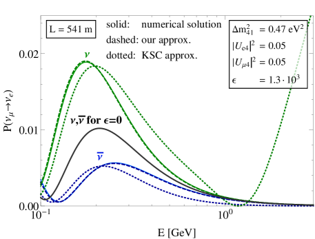
Figure 1: The electron neutrino (green) and anti-neutrino (blue) appearance probability in a model with a large MSW potential in the sterile sector (for instance the baryonic sterile neutrino model from [26]). We use the baseline $L=541$ m and the energy range 0.1–3 GeV of the MiniBooNE experiment and take the favored model parameters from [31]: $\epsilon=G_{B}/(\sqrt{2}G_{F})=1.3\cdot 10^{3}$ ($\Leftrightarrow V_{b}=2\cdot 10^{-10}\,\text{eV}$ for $\rho=3$ g/cm³), $\Delta m_{41}^{2}=0.47$ eV², $|U_{s4}|^{2}=0.9$, $|U_{e4}|^{2}=|U_{\mu 4}|^{2}=0.05$. (We will see below, that this particular parameter point is in fact excluded by MINOS data, though.) For the standard oscillation parameters, we have used the results of the global fit “Free Fluxes and RSBL” of [39]. In black, we show also the prediction of a sterile neutrino model without new interactions ($\epsilon=0$). Dashed lines correspond to our analytic approximations, which coincide with numerical results (solid curves) in this baseline and energy range, while dotted lines show the results from [31].

In the calculation of the analytical formulas in [31] the eigenvalues $\lambda_{i}$ are approximated by setting $A\approx V_{b}+\frac{\Delta m^{2}_{41}}{2E}$ (i.e. taking $|U_{s4}|=1$ in equation (14)). This leads to $\lambda_{1}=\lambda_{2}=\lambda_{3}=0$ and $\lambda_{4}=V_{b}+\Delta m^{2}_{41}/2E$. The oscillation phases of equations (18)–(20) then become $\phi_{1}=\phi_{3}=\frac{1}{2}L(V_{b}+\Delta m_{41}^{2}/2E)$ and $\phi_{2}=0$. With this replacements our equation (15) reduces to equations (21)–(22) in [31]. In the limit of large $V_{b}$ we see from equation (22) that this approximation is only valid if $L/2(1-\lvert U_{s4}\rvert^{2})\Delta m_{41}^{2}/(2E)\ll 1$.

Since the latter condition is fulfilled in the $L/E$ regime at which the LSND and MiniBooNE experiments are sensitive to $\nu_{\mu}\rightarrow\nu_{e}$ flavour transitions, the approximation from [31] is applicable there. This can be seen in figure 1, where the transition probabilities for neutrinos (in green) and anti-neutrinos (in blue) are shown for $L=541$ m and $E=0.1$–3 MeV. We have taken the model parameters at the best fit point from [31] (which we will show to be in fact excluded by MINOS in section III.2). Dashed curves correspond to our analytical approximation (equation (15)), which agrees extremely well with numerical results, while dotted curves show the approximation from equations (21)–(22) of [31]. The difference between the neutrino and anti-neutrino sectors originates from the different signs of the matter potential. As expected, $\epsilon>0$ ($\Leftrightarrow V_{b}>0$) leads to a resonant enhancement of the anti-neutrino transition probabilities and a suppression of the neutrino transition probabilities compared to the case $\epsilon=0$ (black curve). We see that the approximations used in [31] are fairly accurate in the most relevant energy range below 1 GeV, but fail at higher energies.

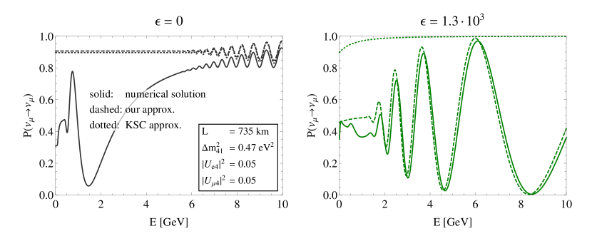
Figure 2: The figure shows the $\nu_{\mu}$ disappearance probability for the MINOS baseline of $L=735\,\text{km}$ and energies up to $10\,\text{GeV}$. We show the survival probability $P_{\nu_{\mu}\rightarrow\nu_{\mu}}$ for $\epsilon=0$ (left panel) and $\epsilon=1.3\cdot 10^{3}$ ($\Leftrightarrow V_{b}=2\cdot 10^{-10}\,\text{eV}$ for $\rho=3$ g/cm³) (right panel) using the best fit parameters from the LSND/MiniBooNE fit of [31]. Solid curves correspond to a numerical calculation in the full four flavour oscillation framework, using for the standard oscillation parameters the values from the fit “Free Fluxes and RSBL” of [39]. Dashed curves show our analytic approximation, equation (17), while dotted curves correspond to equations 20 and 28 of [31]. The comparison shows that, when the new matter potential $V_{b}$ is switched on ($\epsilon>0$), the active-sterile oscillation mode dominates over the standard atmospheric oscillation pattern, an effect which is not captured by the approximations made in [31].

Since standard and non-standard matter effects are most relevant at long baseline ($\gtrsim\text{few}\times 100$ km), it is important to also study the disappearance probability $1-P_{\nu_{\mu}\rightarrow\nu_{\mu}}$ as a function of energy for long-baseline oscillation experiments like MINOS. MINOS has measured $P_{\nu_{\mu}\rightarrow\nu_{\mu}}$ at a baseline of $L=735$ km in the energy range 1–50 GeV. The oscillation probabilities for this baseline and energy range are shown in figure 2 for $\epsilon>0$ (right panel) and also for the Standard Model ($\epsilon=0$, left panel). We see that, due to matter-enhanced oscillations inside the earth, a scenario with strong non-standard matter effects leads to very large muon disappearance even at energies as high as 10 GeV, well above the standard oscillation maximum at $\sim 1.5$ GeV. This is in conflict with MINOS data and we therefore expect that MINOS is able to place very strong constraints on new matter effects in the sterile neutrino sector. Figure 2 also implies that the parameters favored in [31] are ruled out by MINOS.

Comparing numerical results (solid lines) to our analytic approximation (dashed lines), we find, as expected, that the approximations of equations (15) and (17) are accurate at $\Delta m_{31}^{2}L/(2E)\sim 1$ only if $V_{b}$ is very large. We also see that the analytic approximations from [31] (dotted curves in figure 2) are not applicable at long baseline even for large $V_{b}$. For example, in the MINOS case, $\Delta m_{41}^{2}L/(2E)\cdot\,\text{eV}^{2}\sim 100$ for $\Delta m_{41}^{2}\sim\text{eV}^{2}$, the phase $\phi_{2}$ (see equations (19) and (22)) becomes non-negligible. This is the reason why our conclusions regarding the importance of MINOS data for constraining sterile neutrino matter effects differ from those of [31], where $\phi_{2}$ has been neglected.

III Constraints from oscillation experiments

From the analysis in the previous section we expect that the baryonic sterile neutrino model (or models with new sterile neutrino–SM interactions in general) could potentially explain by resonant enhancement an event excess in the MiniBooNE neutrino or anti-neutrino data (but not in both), but is strongly constrained by data from long-baseline experiments. Therefore, we now derive limits on the model using a numerical $\chi^{2}$ analysis of data from MiniBooNE, MINOS and also solar neutrino experiments.

III.1 Analysis method

In our analysis we fix the standard oscillation parameters at their best fit values from the global fit by Gonzalez-Garcia et al. [39] (see table 1) and we assume a normal mass ordering. We have checked that our results for inverted ordering are very similar, with only the solar limits becoming somewhat weaker. (We will comment on this in more detail in section III.2.) For simplicity we set $\delta_{13}=\delta_{14}=\delta_{24}=0$ because none of the experiments considered here is sensitive to CP violation in the small $V_{b}$ limit and equations (15)–(17) show that also the leading terms in the oscillation probabilities for large $V_{b}$ are independent of complex phases. We fix the mixing angle $\theta_{34}=0$ since MiniBooNE is not sensitive to this angle and MINOS has only very limited sensitivity [15]. The impact of $\theta_{34}>0$ on the constraints from solar experiments will be discussed in section III.2. Finally, we set $\sin^{2}2\theta_{14}=0.12$ so that the reactor anomaly [3, 4, 5] can be explained. We will comment on the effect of relaxing this assumption also in section III.2. The constraints we impose on the parameter space are also summarized in table 1. The remaining three parameters $\epsilon=G_{B}/(\sqrt{2}G_{F})$, $\Delta m^{2}_{41}$ and $\theta_{24}$ are scanned over the ranges $\lvert\epsilon\rvert=1-32000$, $\Delta m^{2}_{41}/eV^{2}=0.01-11$ and $\sin^{2}\theta_{24}=0.0001-1$.

$\sin^{2}\theta_{12}$	$\sin^{2}\theta_{23}$	$\sin^{2}\theta_{13}$	$\Delta m_{21}^{2}\,[\text{eV}^{2}]$	$\Delta m_{31}^{2}\,[\text{eV}^{2}]$	$\delta_{13}$, $\delta_{14}$ $\delta_{24}$	$\sin^{2}2\theta_{14}$	$\sin^{2}\theta_{34}$
$0.302$	$0.413$	$0.0227$	$7.5\cdot 10^{-5}$	$2.473\cdot 10^{-3}$	$0$	$0.12$	$0$

Table 1: The parameter values of the baryonic sterile neutrino model that we have fixed in our parameter scan.

We now discuss the details of our fits to MINOS, MiniBooNE and solar neutrino data.

III.1.1 MINOS

For MINOS, we use GLoBES [40, 41] to compute the energy dependent oscillation probabilities $P_{\text{near}}(E)$ for the near detector and $P_{\text{far}}(E)$ for the far detector numerically. We include a low pass filter according to equation (23) with $\sigma_{f}(E)=0.06\cdot E$. The matter density $\rho$ along the neutrino trajectory to the far detector is assumed to be constant at its average value

$$\left\langle\rho_{\text{far}}\right\rangle = \frac{2}{L_{\text{far}}}\int_{\sqrt{R_{\oplus}^{2}-(L_{\text{far}}/2)^{2}}}^{R_{\oplus}}\rho(r)\frac{d}{dr}\Big{(}\sqrt{r^{2}-R_{\oplus}^{2}+(L_{\text{far}}/2)^{2}}\Big{)}dr\text{.}$$ (25)

In this expression, which can be understood from geometric arguments, $r$ is the distance of the neutrino from the center of the earth, $R_{\oplus}$ is the radius of the earth and $L_{\text{far}}=735\,\text{km}$ is the neutrino path length from the source to the far detector [42]. Using the matter density profile from the Preliminary Reference Earth Model (PREM) [43] we obtain $\left\langle\rho_{\text{far}}\right\rangle\approx 2.36\,\text{g}/\text{cm}^{3}$.

For large $V_{b}$, matter effects can be relevant even in the near detector at a baseline $L_{\text{target}}=965\,\text{m}$ from the target. In computing the average matter density $\left\langle\rho\right\rangle_{\text{near}}$ that neutrinos experience on their way to the near detector, we account for the fact that they first travel along the evacuated decay pipe with a length of $L_{\text{pipe}}=675\,\text{m}$. We estimate $\left\langle\rho\right\rangle_{\text{near}}\approx(L_{\text{target}}-L_{\text{pipe}})/L_{\text{near}}\cdot 3\frac{\text{g}}{\text{cm}^{3}}$, where $L_{\text{near}}\simeq 763\,\text{m}$ is the average distance between the neutrino production vertex and the near detector. It is obtained from the decay length of the neutrinos’ parent pions, which have an average energy of $4-5\,\text{GeV}$ [44].

We compute the theoretically predicted event spectrum $N_{\text{osc}}$ by multiplying the ratio $P_{\text{far}}(E)/P_{\text{near}}(E)$ with the background-subtracted prediction for the MINOS event rate in the absence of oscillations, $N_{\text{no osc}}$:

$$N_{\text{osc}}(E)=\big{[}N_{\text{no osc}}(E)-N_{\text{bg}}(E)\big{]}\frac{P_{\text{far}}(E)}{P_{\text{near}}(E)}\text{.}$$ (26)

The no-oscllation rate $N_{\text{no osc}}(E)$ and the background rate $N_{\text{bg}}(E)$ are taken from [45], which is similar to [46] but contains data up to $50\,\text{GeV}$. The higher energy data is important to us since it increases the sensitivity at low matter potential $V_{b}$.

To account for the finite energy resolution of the detector, we fold $N_{\text{osc}}$ with the detector response function $f(E,E^{\prime})$, which maps the true event energy $E^{\prime}$ to the reconstructed energy $E$. Finally, we also add the small experimental background $N_{\text{bg}}(E)$:

$$N_{\text{th}}(E)=N_{\text{bg}}(E)+\int\!f(E,E^{\prime})N_{\text{osc}}(E^{\prime})dE^{\prime}\text{.}$$ (27)

We assume a Gaussian shape for $f(E,E^{\prime})$,

$$f(E,E^{\prime})=\frac{1}{\sigma(E^{\prime})\sqrt{2\pi}}\exp\left(-\frac{(E-E^{\prime})^{2}}{2\sigma^{2}(E^{\prime})}\right)\text{,}$$ (28)

where we choose $\sigma(E^{\prime})=0.2\,\text{GeV}\sqrt{E^{\prime}/\text{GeV}}$. This choice allows us to reproduce the oscillated event rates and the constraints on $\theta_{23}$ and $\Delta m_{31}^{2}$ from [46] with good accuracy. When evaluating equation (27) numerically, we discretize the integral so that $N_{\text{osc}}(E)$ needs to be evaluated only at fixed support points $E_{j}^{\prime}$ with a step size of $\Delta E_{j}^{\prime}=0.25\,\text{GeV}$ in between. (We have checked that choosing a smaller value for $\Delta E_{j}^{\prime}$ does not change our results significantly, which implies that possible aliasing effects are under control.) Following the MINOS analysis [45], events are binned for the analysis according to their reconstructed energy $E$. The rate in th $i$-th bin is given by

$$N_{\text{th}}^{i}=\int_{E_{i}-\Delta E_{i}/2}^{E_{i}+\Delta E_{i}/2}N_{\text{th}}(E)\,dE=N_{\text{bg}}^{i}+\sum_{j}F^{ij}N_{\text{osc}}(E^{\prime}_{j})\text{,}$$ (29)

where $N_{\text{bg}}^{i}$ is the total background in the $i$-th bin and the elements of the detector response matrix $F^{ij}$ are $F^{ij}\equiv=\int_{E_{i}-\Delta E_{i}/2}^{E_{i}+\Delta E_{i}/2}f(E,E_{j}^{\prime})\,dE$. It is important to note that the $F^{ij}$ need to be computed only once.

From equation (29) we compute $\chi^{2}$ according to

$$\chi^{2}=\sum_{i}\Bigg{(}\frac{N_{\text{th}}^{i}-N_{\text{exp}}^{i}}{\sqrt{N_{\text{exp}}^{i}}+0.1\cdot N_{\text{exp}}^{i}}\Bigg{)}^{2}\text{,}$$ (30)

where $N_{\text{exp}}^{i}$ is the observed event rate in the $i$-th energy bin [45] and the sum runs over all energy bins. Note that we have included an additional uncertainty of $10\%$ in order to account for systematic errors without modeling them in detail. Like our choice of $\sigma(E^{\prime})$ in equation (28), also our simplified treatment of systematic errors has been confirmed by cross-checking our simulations against the results of [46, 15].

In figure 3, we compare our prediction for the oscillated neutrino spectrum in MINOS assuming standard 3-flavour oscillations (blue shaded histogram) to the official MINOS prediction (blue unshaded histogram) and to the data (black points with error bars). We find excellent agreement, which validates our calculations. We also show the MINOS no oscillation prediction (red histogram) which is the starting point for our predictions, as well as the survival probability $P_{\nu_{\mu}\to\nu_{\mu}}$ (dashed green line; corresponding vertical scale shown on the right).

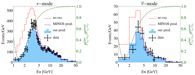
Figure 3: The measured and predicted event spectra for the MINOS ${\nu}_{\mu}$ (left) and $\overline{\nu}_{\mu}$ (right) disappearance measurements. The red histogram is the MINOS prediction assuming no neutrino oscillation [45]. In blue, we show the predicted event spectrum including oscillations according to equation (27), assuming standard three flavour oscillations with the parameters listed in table 1. The blue shaded histogram is our prediction, the unshaded histogram is the prediction by the MINOS collaboration. We overlay the survival probability $P_{\nu_{\mu}\rightarrow\nu_{\mu}}$ (dashed green curve and vertical scale on the right).

III.1.2 MiniBooNE

As for MINOS, the oscillation probabilities for MiniBooNE are calculated numerically in the full four flavour framework with the help of GLoBES [40, 41], including a low pass filter according to equation (23) with $\sigma_{f}(E)=0.06E$. Since the MiniBooNE decay pipe is only 50 m long, while the distance from the target to the detector is $L=541$ m, we neglect the effect of the finite pion decay length. Instead, we take the matter density to be $\left\langle\rho\right\rangle\sim 3\,\text{g}/\text{cm}^{3}$ along the whole neutrino trajectory.

We use a $\chi^{2}$ analysis to compare our predicted oscillation probabilities with the experimentally measured probabilities, which are given in [47] as a function of $L/E$. The data from [47] are shown in figure 4 together with the trivial no-oscillation prediction and with our prediction for the MiniBooNE best fit points in the baryonic sterile neutrino scenario for $\epsilon>0$ and $\epsilon<0$.

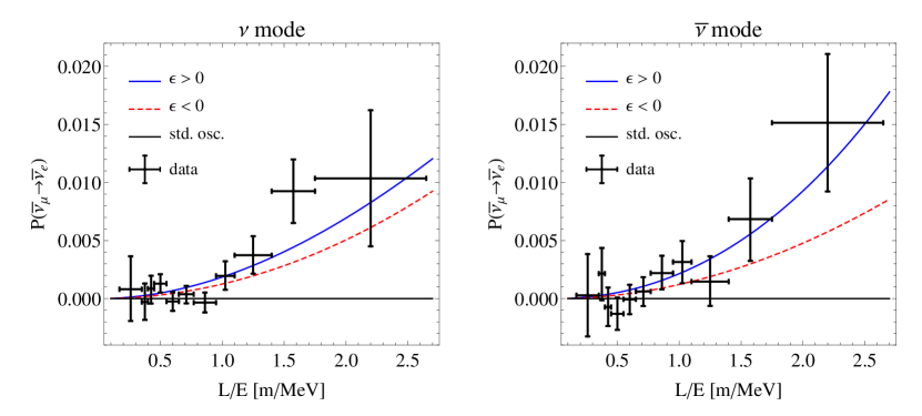
Figure 4: The measured MiniBooNE $\nu_{\mu}\to\nu_{e}$ (left) and $\bar{\nu}_{\mu}\to\bar{\nu}_{e}$ (right) appearance probabilities compared to the predictions of the baryonic sterile neutrino scenario for $\epsilon>0$ (blue line) and $\epsilon<0$ (dashed red line) at the MiniBooNE best fit points from table 2. Without sterile neutrinos, the appearance probability at the MiniBooNE baseline is approximately zero (solid black line).

III.1.3 Solar neutrinos

We analyze solar neutrino oscillation data by comparing the measured $\nu_{e}$ survival probability $P_{\nu_{e}\to\nu_{e}}$ at different energies to our theoretical predictions. The data points are taken from [48] and include results from Super-Kamiokande, SNO, Borexino and radiochemical experiments.

In calculating $P_{\nu_{e}\to\nu_{e}}$, we assume MSW flavour transitions to be fully adiabatic and we account for the fact that solar neutrinos arrive at the earth as an incoherent mixture of mass eigenstates. We obtain $P_{\nu_{e}\to\nu_{e}}$ according to

$$P_{\nu_{e}\rightarrow\nu_{e}}=\sum_{i}\lvert U_{ei}\rvert^{2}\cdot\lvert\tilde{U}_{ei}(0)\rvert^{2}\text{,}$$ (31)

where $\tilde{U}_{ei}(0)$ is the mixing matrix in matter at the center of the Sun ($t=0$) and $U_{ei}$ is the vacuum mixing matrix. We neglect earth matter effects here, but we have checked that, in the parameter ranges of interest to us, the day–night effect caused by the earth matter is of the order of few per cent, comparable to the day–night effect in the Standard Model. We thus anticipate that our limits would only change marginally if Earth matter effects were included.

In order to verify that the assumption of full adiabaticity is justified, we have examined the adiabaticity parameter $\gamma$ in the two flavour approximation and we have checked that the adiabaticity condition [32]

$$\gamma^{-1}=\frac{\sin 2\theta\frac{\Delta m_{ij}^{2}}{2E}}{\lvert\lambda_{i}-\lambda_{j}\rvert^{3}}\cdot\bigg{|}\frac{dV_{b}}{dt}\bigg{|}\ll 1$$ (32)

holds for all relevant mass squared difference $\Delta m_{ij}^{2}$ even for large $V_{b}$ and the smallest relevant differences between the Hamiltonian eigenvalues $\lambda_{i}$ and $\lambda_{j}$, which occur at the resonance position. We determine the derivative of the matter potential, $\big{|}dV_{b}/dt\big{|}$, from the solar density profile of the standard solar model BS’05 (OP) [49].

In figure 5, we compare the measured solar neutrino oscillation probabilities $P_{\nu_{e}\to\nu_{e}}$ to the theoretical predictions for standard three flavour oscillations and for the best fitting baryonic neutrino scenarios with $\epsilon>0$ (blue) and $\epsilon<0$ (red).

We observe that for $\epsilon<0$, a peak-like structure appears in $P_{\nu_{e}\to\nu_{e}}$, which suggests that mixing of $\nu_{e}$ with other flavors is dynamically driven to zero for specific parameter combinations. The peak occurs at parameter points where $\Delta m_{41}^{2}/(2E),\ \Delta m_{31}^{2}/(2E)\gg\Delta m_{21}^{2}/(2E)$, $V_{b}$ and where moreover $\theta_{34}$ and $\theta_{13}$ are small. To understand its origin, it is therefore helpful to determine the eigenvalues of the Hamiltonian $H_{\text{eff}}^{\text{flavor}}$ (see equation (10)) using time-independent perturbation theory, with the zeroth order Hamiltonian given by

$$H_{\text{eff}}^{\text{flavour,(0)}}\equiv\frac{1}{2E}U\text{diag}(0,0,\Delta m_{31}^{2},\Delta m_{41}^{2})U^{\dagger}\,,$$ (33)

and the perturbation being $H_{\text{eff}}^{\text{flavour,(1)}}\equiv H_{\text{eff}}^{\text{flavour}}-H_{\text{eff}}^{\text{flavour,(0)}}$. In the approximation $\theta_{34}=\theta_{13}=0$, a set of zeroth order eigenvectors is obviously given by the matrix $U^{(0)}\equiv R_{24}^{\prime}R_{14}^{\prime}R_{23}$, where, as before, $R_{ij}$ and $R_{ij}^{\prime}$ are real and complex rotation matrices, respectively. Since $H_{\text{eff}}^{\text{flavour,(0)}}$ has zero as a double eigenvalue, we next have to find eigenvectors of $H_{\text{eff}}^{\text{flavour,(1)}}$ in the subspace corresponding to this double eigenvalue. In other words, we need to compute $U^{(0){\dagger}}H_{\text{eff}}^{\text{flavour,(1)}}U^{(0)}$ and then diagonalize the upper left $2\times 2$ block. It turns out that, if the condition

$$\frac{\Delta m_{21}^{2}}{2E}\sin 2\theta_{12}+V_{b}\cos\theta_{23}\sin\theta_{14}\sin 2\theta_{24}\simeq 0$$ (34)

is fulfilled, this $2\times 2$ block is automatically diagonal. This implies that $U^{(0)}(1,0,0,0)^{T}\simeq(1,0,0,0)$ is an approximate eigenvector of $H_{\text{eff}}^{\text{flavour}}$. Hence, if (34) holds at the center of the Sun, solar neutrinos are produced in an almost pure $\nu_{1}$ mass eigenstate. After adiabatic flavour conversion, the resulting $\nu_{e}$ admixture is of order $\cos\theta_{12}^{2}$, leading to a peak in the observed solar neutrino spectrum at Earth.

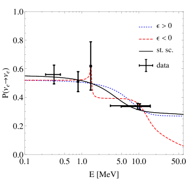
Figure 5: Comparison of the measured solar neutrino oscillation probabilities to our theoretical predictions for standard three flavour oscillations (black) and for the best fit parameter points of the baryonic sterile neutrino model with $\epsilon>0$ (dotted blue) and $\epsilon<0$ (dashed red).

III.2 Results

In figures 6 and 7 our constraints on the parameter space of baryonic sterile neutrinos are presented as contour plots for $\epsilon>0$ and $\epsilon<0$, respectively. We show exclusion limits (lines of constant $\chi^{2}-\chi^{2}_{\text{min}}$) at the 95% and $3\sigma$ confidence levels. In each panel, we keep either $\epsilon$ or $\Delta m_{41}^{2}$ fixed at the value indicated in the plot and show constraints on the remaining two parameters. Moreover, as discussed in section III.1, we fixed $\sin^{2}2\theta_{14}=0.12$. Blue lines correspond to constraints from solar experiments, black lines are the limits from MINOS and the colored regions show the parameter region preferred by MiniBooNE. The best fit values for $\epsilon>0$ and $\epsilon<0$ are listed in table 2.

		$\epsilon=G_{B}/(\sqrt{2}G_{F})$	$\Delta m_{41}^{2}\,[\text{eV}^{2}]$	$\sin^{2}\theta_{24}$	$\chi^{2}_{\text{min}}/\text{d.o.f.}$
MINOS	$\epsilon>0$	$16.9$	$0.014$	$0.0024$	$37.7/49$
	$\epsilon<0$	$-19.2$	$0.037$	$0.00083$	$36.1/49$
MiniBooNE	$\epsilon>0$	$30634$	$0.316$	$0.10$	$16.1/20$
	$\epsilon<0$	$-32000$	$0.116$	$0.75$	$16.4/20$
Solar	$\epsilon>0$	$0.20$	insensitive	$1.0$	$1.10/3$
	$\epsilon<0$	$-38.0$	$0.013$	$0.046$	$0.41/3$

Table 2: Best fit values resulting from our parameter scan for the different experimental data sets. For the MiniBooNE fit with $\epsilon<0$ analysis the best fit value for $\epsilon$ is located outside the boundary of the analysis region, but $\chi^{2}$ hardly depends on $\lvert\epsilon\rvert$ in this region. Also note that the solar best fit in the $\epsilon>0$ case has $\epsilon<1$ and is not sensitive to the exact value of $\Delta m_{41}^{2}$ in the interval $[0.01,11]$.

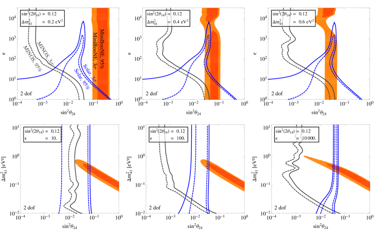
Figure 6: 95% and $3\sigma$ confidence level constraints on the parameters $\Delta m_{41}^{2}$, $\sin^{2}2\theta_{24}$ and $\epsilon$ (strength of the new MSW potential) of the baryonic sterile neutrino model in the $\epsilon>0$ case. Blue contours show constraints from solar experiments, black contours are for MINOS and shaded areas correspond to the region preferred by MiniBooNE. We have fixed $\sin^{2}2\theta_{14}=0.12$, as motivated by the reactor and gallium anomalies.

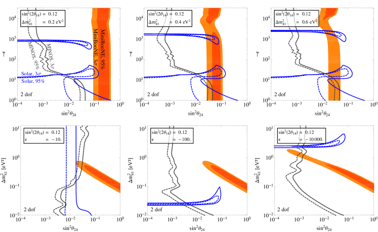
Figure 7: 95% and $3\sigma$ confidence level constraints on the parameters $\Delta m_{41}^{2}$, $\sin^{2}2\theta_{24}$ and $\epsilon$ (strength of the new MSW potential) of the baryonic sterile neutrino model in the $\epsilon<0$ case. Blue contours show constraints from solar experiments, black contours are for MINOS and shaded areas correspond to the region preferred by MiniBooNE. We have fixed $\sin^{2}2\theta_{14}=0.12$, as motivated by the reactor and gallium anomalies.

We see that values of $|\epsilon|\gtrsim 10$ are strongly disfavored by MINOS except in the case of tiny active–sterile mixing angles. For such large values of $\epsilon$, the new MSW resonance at $\Delta m_{41}^{2}/(2E)\sim V_{b}$ lies within the MINOS energy range $E<50$ GeV and leads to a constraint $\sin^{2}\theta_{24}\lesssim 10^{-3}$. Such small mixing angles are, however, irrelevant for possible explanations of MiniBooNE and other short-baseline anomalies. The MINOS contours also show that in most of the mass range $10^{-2}\ \text{eV}^{2}\lesssim\Delta m_{41}^{2}\lesssim 10^{1}\ \text{eV}^{2}$, values of $\sin^{2}\theta_{24}\gtrsim 0.01$ are excluded, with limits becoming much stronger at large $\epsilon$.

Solar neutrinos also have some sensitivity to $\theta_{24}$, but limits on $\epsilon$ vary a lot with $\sin^{2}\theta_{24}$. For intermediate values $0.01\lesssim\sin^{2}\theta_{24}\lesssim 0.1$, even values of $|\epsilon|$ as large as $\text{few}\times 10^{3}$ are compatible with solar neutrino data. For $\epsilon>0$, we notice that solar limits on $\epsilon$ are weakest at $\sin^{2}\theta_{24}\sim\text{few}\times 10^{-2}$. In this regime, the additional neutrino disappearance due to nonzero $\theta_{14}$ and $\theta_{24}$ is partially compensated by $V_{b}$-induced modifications to the MSW resonance structure. In particular, the 1–4 and 2–4 mixings imply that above the solar MSW resonance, $\nu_{1}$–$\nu_{2}$ mixing is not as strongly suppressed as in the standard case. This reduces the flavour transition probability at energies above the resonance. Note that this effect is related to a sterile neutrino-induced smearing of the atmospheric resonance (which at the center of the Sun lies at about 200 MeV) to the extent that it has a small impact even at energies as low as $\sim 10$ MeV. The effect is therefore absent if the neutrino mass ordering is inverted so that the atmospheric resonance lies in the anti-neutrino sector. We have checked that indeed the limits on $\epsilon$ from solar neutrino experiments become somewhat weaker in this case. For $\epsilon<0$, the exclusion contours reveal an allowed “island” at $\epsilon\sim-10^{3}$. In the parameter region corresponding to these islands, the non-standard MSW resonance at $\Delta m_{41}^{2}/2E\simeq V_{b}$ mimics the effect of the standard solar resonance. Also, in this parameter region, the atmospheric MSW resonance—modified by the presence of the sterile neutrinos—has a small impact. Therefore, the “islands” move down by almost an order of magnitude in $|\epsilon|$ if the neutrino mass ordering is inverted. The $\Delta m_{41}^{2}$-independent “peninsula” at $\epsilon\sim-20$, is related to the appearance of the peak structure in $P_{\nu_{e}\to\nu_{e}}$ which we discussed in section III.1.3 and which is independent of the mass ordering.

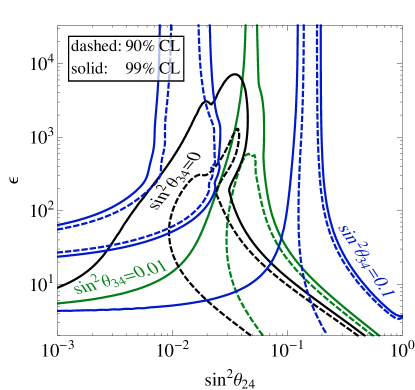
Figure 8: Constraints on $\epsilon$ and $\sin^{2}\theta_{24}$ from solar neutrinos for fixed $\sin^{2}2\theta_{14}=0.12$ (as motivated by the reactor and gallium anomalies), but for different values of $\theta_{34}$. The value of $\Delta m_{41}^{2}$ has been marginalized over in the range $10^{-2}\leq\Delta m_{41}^{2}\leq 1.1\cdot 10^{1}$.

The allowed parameter region for the measured appearance signal in MiniBooNE is very similar to the one obtained in conventional sterile neutrino scenarios (see for instance the analysis by the MiniBooNE collaboration themselves [2]) with the exception that for large matter potentials, the allowed region is expanded towards lower $\sin^{2}\theta_{24}$ and higher $\Delta m^{2}_{41}$.

We now relax our assumption $\theta_{34}=0$. The main sensitivity to $\theta_{34}$ is expected to come from solar neutrinos [15] (and from MINOS neutral current measurements, which we did not consider in this work, though). We compare the solar neutrino limits in the $\sin^{2}\theta_{24}$–$\epsilon$ plane for different values of $\theta_{34}$ in figure 8, marginalizing over the sterile neutrino mass in the range $10^{-2}\leq\Delta m_{41}^{2}\leq 1.1\cdot 10^{1}$. We see that the constraints on $\epsilon$ become somewhat weaker if $\sin^{2}\theta_{34}\sim 0.01$ and change significantly for larger values of $\sin^{2}\theta_{34}$. This implies that, for large $\theta_{34}$, a scenario with strong non-standard matter potential can be consistent with solar data and with MiniBooNE. Nevertheless, such a scenario would still be ruled out by MINOS.

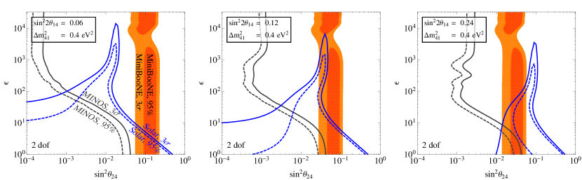
Figure 9: The effect of varying $\theta_{14}$ on the constraints in the $\sin^{2}\theta_{24}$–$\epsilon$ plane. The plot in the center reproduces middle panel in the upper row of figure 6, while the left and right panels show similar constraints for smaller and larger $\theta_{14}$, respectively.

Finally, let us also discuss the effect of choosing $\sin^{2}2\theta_{14}$ different from the value 0.12 preferred by the reactor neutrino anomaly. To this end, we show in figure 9 how the constraints on $\epsilon$ and $\theta_{24}$ for fixed $\Delta m_{41}^{2}$ are modified if $\sin^{2}2\theta_{14}$ is taken a factor of 2 smaller (left panel) or a factor of 2 larger (right panel) than the preferred value. We see that the MiniBooNE preferred region, which is sensitive only to the combination $\sin^{2}2\theta_{14}\sin^{2}\theta_{24}$ is simply shifted by a factor of 2. Solar limits are affected in a less trivial way and we find that at large $\theta_{14}$, there is even a preference for nonzero $\theta_{24}$. Note, however, that the goodness of fit becomes slightly worse as $\theta_{14}$ is increased: the minimum $\chi^{2}/\text{dof}$ is 0.8/3 for $\sin^{2}2\theta_{14}=0.6$ and 2.7/3 for $\sin^{2}2\theta_{14}=0.24$. Finally, MINOS limits are weakened if $\theta_{14}$ is large, especially at large $\epsilon$. This happens because a larger mixing between $\nu_{e}$ and $\nu_{b}$ by unitarity implies more $\nu_{\mu}$ disappearance.

IV Conclusions

To summarize, we have derived constraints on models with extended sterile neutrino sectors that feature in particular a new gauge interaction between sterile neutrinos and SM particles. As a specific example, we have considered a scenario in which eV-scale sterile neutrinos are charged under gauged baryon number $U(1)_{B}$. In principle, such interactions could be several orders of magnitude stronger than SM weak interactions, so the Mikheyev-Smirnov-Wolfenstein (MSW) potentials they generate could be significantly larger than the matter potential in standard three-flavour neutrino oscillations.

We have also computed approximate analytic expressions for the relevant oscillation probabilities in matter, improving and extending the expressions previously derived in [31]. We have then numerically analyzed data from the MINOS experiment, from solar neutrino measurements and from MiniBooNE to show that new gauge interactions in the sterile neutrino sector cannot be large unless the active–sterile neutrino mixing is very small. In particular, if the ratio $\epsilon$ of the non-standard and standard matter potentials is larger than $\sim 10$, MINOS excludes mixing angles down to $\sin^{2}2\theta_{24}\sim 10^{-3}$. (This limit becomes stronger if $\theta_{14}=0$.)

We conclude that sterile neutrino searches in oscillation experiments are powerful tools to constrain certain models with hidden sector gauge interactions. We also conclude that such models do not help to resolve the tension in the global fit to short-baseline oscillation data.

Comparing to the interaction strength required for baryonic sterile neutrinos to yield signals in dark matter detectors [26, 27, 28, 29], we conclude that in the case of eV scale sterile neutrinos, baryonic interactions cannot be large enough to be observable in the current generation of experiments. On the other hand, interesting signals may still be possible in future ton-scale experiments.

References

- Aguilar et al. [2001] A. Aguilar et al. (LSND), Phys. Rev. D64, 112007 (2001), eprint hep-ex/0104049.
- Aguilar-Arevalo et al. [2012] A. Aguilar-Arevalo et al. (MiniBooNE Collaboration) (2012), eprint 1207.4809.
- Mueller et al. [2011] T. Mueller, D. Lhuillier, M. Fallot, A. Letourneau, S. Cormon, et al., Phys.Rev. C83, 054615 (2011), eprint 1101.2663.
- Mention et al. [2011] G. Mention, M. Fechner, T. Lasserre, T. Mueller, D. Lhuillier, et al., Phys.Rev. D83, 073006 (2011), eprint 1101.2755.
- Huber [2011] P. Huber, Phys.Rev. C84, 024617 (2011), eprint 1106.0687.
- Hayes et al. [2013] A. Hayes, J. Friar, G. Garvey, and G. Jonkmans (2013), eprint 1309.4146.
- Acero et al. [2008] M. A. Acero, C. Giunti, and M. Laveder, Phys.Rev. D78, 073009 (2008), eprint 0711.4222.
- Giunti and Laveder [2011a] C. Giunti and M. Laveder, Phys.Rev. C83, 065504 (2011a), eprint 1006.3244.
- Kopp et al. [2011] J. Kopp, M. Maltoni, and T. Schwetz, Phys.Rev.Lett. 107, 091801 (2011), eprint 1103.4570.
- Giunti and Laveder [2011b] C. Giunti and M. Laveder, Phys.Lett. B706, 200 (2011b), eprint 1111.1069.
- Karagiorgi [2011] G. Karagiorgi (2011), eprint 1110.3735.
- Giunti and Laveder [2011c] C. Giunti and M. Laveder, Phys.Rev. D84, 093006 (2011c), eprint 1109.4033.
- Giunti and Laveder [2011d] C. Giunti and M. Laveder, Phys.Rev. D84, 073008 (2011d), eprint 1107.1452.
- Abazajian et al. [2012] K. Abazajian, M. Acero, S. Agarwalla, A. Aguilar-Arevalo, C. Albright, et al. (2012), eprint 1204.5379.
- Kopp et al. [2013] J. Kopp, P. A. N. Machado, M. Maltoni, and T. Schwetz, JHEP 1305, 050 (2013), eprint 1303.3011.
- Ade et al. [2013] P. Ade et al. (Planck Collaboration) (2013), eprint 1303.5076.
- Ade et al. [2014] P. Ade et al. (BICEP2 Collaboration) (2014), eprint 1403.3985.
- Giusarma et al. [2014] E. Giusarma, E. Di Valentino, M. Lattanzi, A. Melchiorri, and O. Mena (2014), eprint 1403.4852.
- Dvorkin et al. [2014] C. Dvorkin, M. Wyman, D. H. Rudd, and W. Hu (2014), eprint 1403.8049.
- Li et al. [2014] H. Li, J.-Q. Xia, and X. Zhang (2014), eprint 1404.0238.
- Zhang et al. [2014] J.-F. Zhang, Y.-H. Li, and X. Zhang (2014), eprint 1403.7028.
- Archidiacono et al. [2014] M. Archidiacono, N. Fornengo, S. Gariazzo, C. Giunti, S. Hannestad, et al. (2014), eprint 1404.1794.
- Hannestad et al. [2014] S. Hannestad, R. S. Hansen, and T. Tram, Phys.Rev.Lett. 112, 031802 (2014), eprint 1310.5926.
- Dasgupta and Kopp [2014] B. Dasgupta and J. Kopp, Phys.Rev.Lett. 112, 031803 (2014), eprint 1310.6337.
- Bringmann et al. [2013] T. Bringmann, J. Hasenkamp, and J. Kersten (2013), eprint 1312.4947.
- Pospelov [2011] M. Pospelov, Phys.Rev. D84, 085008 (2011), eprint 1103.3261.
- Harnik et al. [2012] R. Harnik, J. Kopp, and P. A. Machado, JCAP 1207, 026 (2012), eprint 1202.6073.
- Pospelov and Pradler [2012] M. Pospelov and J. Pradler, Phys.Rev. D85, 113016 (2012), eprint 1203.0545.
- Pospelov and Pradler [2013] M. Pospelov and J. Pradler (2013), eprint 1311.5764.
- Ho and Scherrer [2013] C. M. Ho and R. J. Scherrer, Phys.Rev. D87, 065016 (2013), eprint 1212.1689.
- Karagiorgi et al. [2012] G. Karagiorgi, M. Shaevitz, and J. Conrad (2012), eprint 1202.1024.
- Akhmedov [1999] E. K. Akhmedov (1999), eprint hep-ph/0001264.
- Giunti and Kim [2007] C. Giunti and C. W. Kim, Fundamentals of Neutrino Physics and Astrophysics (OUP Oxford, New York, 2007).
- Aguilar-Arevalo et al. [2007] A. Aguilar-Arevalo et al. (The MiniBooNE Collaboration), Phys.Rev.Lett. 98, 231801 (2007), eprint 0704.1500.
- Aguilar-Arevalo et al. [2009] A. Aguilar-Arevalo et al. (MiniBooNE Collaboration), Phys.Rev.Lett. 103, 111801 (2009), eprint 0904.1958.
- Aguilar-Arevalo et al. [2010] A. Aguilar-Arevalo et al. (The MiniBooNE Collaboration), Phys.Rev.Lett. 105, 181801 (2010), eprint 1007.1150.
- Huber et al. [2013] P. Huber, J. Kopp, M. Lindner, M. Rolinec, and W. Winter, Globes manual (2013), URL http://www.mpi-hd.mpg.de/personalhomes/globes/documentation/g%lobes-manual-3.0.8.pdf.
- Beuthe [2003] M. Beuthe, Phys.Rept. 375, 105 (2003), eprint hep-ph/0109119.
- Gonzalez-Garcia et al. [2012] M. Gonzalez-Garcia, M. Maltoni, J. Salvado, and T. Schwetz, JHEP 1212, 123 (2012), eprint 1209.3023.
- Huber et al. [2005] P. Huber, M. Lindner, and W. Winter, Comput.Phys.Commun. 167, 195 (2005), eprint hep-ph/0407333.
- Huber et al. [2007] P. Huber, J. Kopp, M. Lindner, M. Rolinec, and W. Winter, Comput.Phys.Commun. 177, 432 (2007), eprint hep-ph/0701187.
- Michael et al. [2006] D. Michael et al. (MINOS Collaboration), Phys.Rev.Lett. 97, 191801 (2006), eprint hep-ex/0607088.
- Anderson [1989] D. Anderson, Theory of the Earth (Blackwell Scientific Publications, 1989), ISBN 978-0-865-42123-3.
- Diwan et al. [2004] M. Diwan, B. Viren, D. Harris, A. Marchionni, J. Morfin, et al. (2004).
- de Jong [2013] J. de Jong (MINOS Collaboration), Nucl.Phys.Proc.Suppl. 237-238, 166 (2013).
- Adamson et al. [2013] P. Adamson et al. (MINOS Collaboration), Phys.Rev.Lett. 110, 251801 (2013), eprint 1304.6335.
- Aguilar-Arevalo et al. [2013] A. Aguilar-Arevalo et al. (MiniBooNE Collaboration), Phys.Rev.Lett. 110, 161801 (2013), eprint 1207.4809.
- Bellini et al. [2013] G. Bellini et al. (Borexino Collaboration) (2013), eprint 1308.0443.
- Bahcall et al. [2005] J. N. Bahcall, A. M. Serenelli, and S. Basu, Astrophys.J. 621, L85 (2005), eprint astro-ph/0412440.