Computation of potentials from current electrodes in cylindrically stratified media: A stable, rescaled semi-analytical formulation

Abstract

We present an efficient and robust semi-analytical formulation to compute the electric potential due to arbitrary-located point electrodes in three-dimensional cylindrically stratified media, where the radial thickness and the medium resistivity of each cylindrical layer can vary by many orders of magnitude. A basic roadblock for robust potential computations in such scenarios is the poor scaling of modified-Bessel functions used for computation of the semi-analytical solution, for extreme arguments and/or orders. To accommodate this, we construct a set of rescaled versions of modified-Bessel functions, which avoids underflows and overflows in finite precision arithmetic, and minimizes round-off errors. In addition, several extrapolation methods are applied and compared to expedite the numerical evaluation of the (otherwise slowly convergent) associated Sommerfeld-type integrals. The proposed algorithm is verified in a number of scenarios relevant to geophysical exploration, but the general formulation presented is also applicable to other problems governed by Poisson equation such as Newtonian gravity, heat flow, and potential flow in fluid mechanics, involving cylindrically stratified environments.

1 Introduction

Resistivity logging is extensively used for detecting, characterizing, and analyzing hydrocarbon-bearing zones in the subsurface earth [30, 17, 7, 4, 13, 14, 35, 3]. This sensing modality employs electrode-type devices mounted on a mandrel that inject electric currents into the surrounding earth formation [5, 29]. The ensuing electric potential is then measured at different locations to provide estimates for the surrounding resistivity. Many numerical techniques such as finite-differences, finite elements, numerical mode-matching, and finite volumes method can be used to model the response of resistivity logging tools  [12, 8, 10, 26, 23, 24, 20, 25, 21, 22, 11, 6, 9]. Brute-force techniques are rather versatile and applicable to arbitrary resistivity distributions; however, at the same time, this precludes optimality in particular cases of special interest, such as when resistivity logging environment can be represented as a cylindrically stratified medium [2]. Depending on the implementation, brute-force techniques may have difficulties handling extreme sharp discontinuities in the coefficients, as is the case for the resistivity parameter for the physical scenario considered here, which can change by many orders of magnitude across adjacent layers.

In this paper, a robust semi-analytical formulation for computing the electric potential due to arbitrary-located point electrodes in three-dimensional cylindrically stratified media is proposed. The present formulation is based on a series expansion in terms of azimuth Fourier modes and a spectral integral over the vertical wavenumber along the axial direction. The resulting problem in terms of the radial variable yields a set of modified Bessel equations. The present formulation removes roadblocks for numerical computations associated with the poor scaling of modified-Bessel functions for very small and/or very large arguments and/or orders [27, 31, 1]. This is done by constructing a set of rescaled, modified-Bessel functions that can be stably evaluated under double-precision arithmetic, akin to what has been done in the past for ordinary (non-modified) Bessel functions [16] . The present formulation also carefully manipulates the analytical formulae for the potential in such media to yield a set of integrand expressions can be computed in a robust manner under double-precision for a wide range of layer thicknesses, layer resistivities, and source and observation point separations. Finally, a number of acceleration techniques are implemented and compared to effect the efficient numerical integration of the Sommerfeld-type (spectral) integrals, which otherwise suffer from slow convergence. The proposed algorithm is verified in a number of practical scenarios relevant to geophysical exploration. More generally, the mathematical setting here corresponds to the classical problem of obtaining the Green’s function for the steady diffusion equation (Poisson problem) with discontinuous coefficients in a separable geometry. As such, the general formalism presented here is also applicable to other problems governed by Poisson equation such as Newtonian gravity, heat flow, elasticity, neutron transport, and potential flows in fluid mechanics, in cylindrically stratified geometries.

2 Formulation

2.1 Electric potential in homogeneous media

In a homogeneous medium, the electric potential $\psi$ from a current electrode at the origin writes as [31]

$$\psi=\frac{\mathcal{I}}{4\pi\sigma\sqrt{\rho^{2}+z^{2}}}=\frac{\mathcal{I}}{2\pi^{2}\sigma}\int_{0}^{\infty}K_{0}(\lambda\rho)\cos(\lambda z)d\lambda,$$ (1)

where $\mathcal{I}$ is the electric current flowing into the medium from the electrode, $\sigma$ is the conductivity of the medium, and $K_{0}(\cdot)$ is the modified-Bessel function of the second kind of the zeroth order. For the second equality, the complete Lipschitz-Hankel integral [32] is employed. When the source is off the origin, higher order azimuthal modes appear. Using the addition theorem for $K_{0}$, (1) is modified to

$$\psi =\frac{\mathcal{I}}{2\pi^{2}\sigma}\int_{0}^{\infty}K_{0}(\lambda|\boldsymbol{\rho}-\boldsymbol{\rho^{\prime}}|)\cos(\lambda(z-z^{\prime}))d\lambda$$

$$=\frac{\mathcal{I}}{2\pi^{2}\sigma}\sum_{n=-\infty}^{\infty}e^{\mathrm{i}n(\phi-\phi^{\prime})}\int_{0}^{\infty}I_{n}(\lambda\rho_{<})K_{n}(\lambda\rho_{>})\cos(\lambda(z-z^{\prime}))d\lambda,$$ (2)

in terms of modified-Bessel functions of both first, $I_{n}(\cdot)$ and second, $K_{n}(\cdot)$, kinds. In the above, primed coordinates ($\rho^{\prime},\phi^{\prime},z^{\prime}$) represent the source location and unprimed coordinates ($\rho,\phi,z$) represent the observation point. Also, $\rho_{<}=\min(\rho,\rho^{\prime})$ and $\rho_{>}=\max(\rho,\rho^{\prime})$.

2.2 Electric potential in cylindrically stratified media

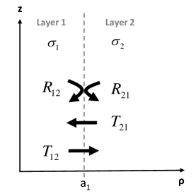
Figure 1: Schematic description of two layers with associated coefficients in the $\rho z$-plane.

In a cylindrically stratified medium, boundary conditions at the interfaces need to be incorporated. Let us first consider the case with two distinct cylindrical layers, as depicted in Fig. 1. When the source is embedded in layer 1, we denote it the outgoing-potential case. In this case, the primary potential $\psi^{p}$ is a function of $K_{n}(\lambda\rho)$ because $I_{n}(\lambda\rho)$ diverges as $\rho$ goes to infinity. On the other hand, when the source is embedded in layer 2, we denote it the standing-potential case and $\psi^{p}$ is a function of $I_{n}(\lambda\rho)$ instead of $K_{n}(\lambda\rho)$ because $K_{n}(\lambda\rho)$ diverges when $\rho$ goes to zero. For the outgoing-potential case, the $n$-th harmonic with $e^{\mathrm{i}n(\phi-\phi^{\prime})}$ dependence in layer 1 and layer 2 can be expressed, resp., as

$$\psi_{1} =\left[K_{n}(\lambda\rho)+R_{12}I_{n}(\lambda\rho)\right]A_{0},$$ (3a)

$$\psi_{2} =T_{12}K_{n}(\lambda\rho)A_{0},$$ (3b)

where $R_{12}$ and $T_{12}$ are the (local) reflection and transmission coefficients at the boundary $a_{1}$, and $A_{0}$ is an arbitrary amplitude of the primary potential. Applying the boundary conditions [31] at the interface, we obtain

$$R_{12} =\frac{(\sigma_{2}-\sigma_{1})K_{n}(\lambda a_{1})K^{\prime}_{n}(\lambda a_{1})}{\sigma_{1}I^{\prime}_{n}(\lambda a_{1})K_{n}(\lambda a_{1})-\sigma_{2}I_{n}(\lambda a_{1})K^{\prime}_{n}(\lambda a_{1})},$$ (4a)

$$T_{12} =\frac{\sigma_{1}}{\lambda a_{1}\left[\sigma_{1}I^{\prime}_{n}(\lambda a_{1})K_{n}(\lambda a_{1})-\sigma_{2}I_{n}(\lambda a_{1})K^{\prime}_{n}(\lambda a_{1})\right]}.$$ (4b)

For the standing-potential case, we similarly have

$$\psi_{1} =T_{21}I_{n}(\lambda\rho)B_{0},$$ (5a)

$$\psi_{2} =\left[R_{21}K_{n}(\lambda\rho)+I_{n}(\lambda\rho)\right]B_{0},$$ (5b)

and

$$R_{21} =\frac{(\sigma_{2}-\sigma_{1})I_{n}(\lambda a_{1})I^{\prime}_{n}(\lambda a_{1})}{\sigma_{1}I^{\prime}_{n}(\lambda a_{1})K_{n}(\lambda a_{1})-\sigma_{2}I_{n}(\lambda a_{1})K^{\prime}_{n}(\lambda a_{1})},$$ (6a)

$$T_{21} =\frac{\sigma_{2}}{\lambda a_{1}\left[\sigma_{1}I^{\prime}_{n}(\lambda a_{1})K_{n}(\lambda a_{1})-\sigma_{2}I_{n}(\lambda a_{1})K^{\prime}_{n}(\lambda a_{1})\right]}.$$ (6b)

When more than two distinct layers are present, multiple reflections and transmissions occur. Therefore, generalized reflection and transmission coefficients should be determined. The procedure to obtain these coefficients is very similar to the one used for time-harmonic case in [2] and will not be derived in detail here. Fig. 2 depicts the relevant coefficients to the outgoing-potential case in the medium consisting of three cylindrical layers. The potentials in the three layers can be expressed as

$$\psi_{1} =\left[K_{n}(\lambda\rho)+\widetilde{R}_{12}I_{n}(\lambda\rho)\right]A_{1},$$ (7a)

$$\psi_{2} =\left[K_{n}(\lambda\rho)+R_{23}I_{n}(\lambda\rho)\right]A_{2},$$ (7b)

$$\psi_{3} =T_{23}K_{n}(\lambda\rho)A_{3}.$$ (7c)

Applying proper constraint equations, we obtain

$$\widetilde{R}_{12}=R_{12}+T_{21}R_{23}(1-R_{21}R_{23})^{-1}T_{12}.$$ (8)

If another layer is added beyond layer 3, only $R_{23}$ needs to be replaced by $\widetilde{R}_{23}$. Therefore, the generalized reflection coefficient in cylindrically stratified media for the outgoing-potential case is

$$\widetilde{R}_{i,i+1}=R_{i,i+1}+T_{i+1,i}\widetilde{R}_{i+1,i+2}(1-R_{i+1,i}\widetilde{R}_{i+1,i+2})^{-1}T_{i,i+1}.$$ (9)

All amplitudes $A_{i}$’s as well as generalized reflection coefficients should be determined in order to obtain the potential everywhere. The relationship between two successive amplitudes in cylindrically stratified media can be written as

$$A_{i+1}=T_{i,i+1}A_{i}+R_{i+1,i}R_{i+1,i+2}A_{i+1}.$$ (10)

From (10), a new coefficient denoted by $S$ is defined as

$$S_{i,i+1}=(1-R_{i+1,i}\widetilde{R}_{i+1,i+2})^{-1}T_{i,i+1}$$ (11)

such that $A_{i+1}=S_{i,i+1}A_{i}$. The above coefficient can be regarded as a ‘local’ transmission coefficient between two adjacent layers, as depicted in Fig. 2b. Generalized transmission coefficient described in Fig. 3 can be defined using the $S$-coefficients (11) through

$$\widetilde{T}_{ji}=T_{i-1,i}S_{i-2,i-1}\cdots S_{j,j+1}=T_{i-1,i}\prod_{k=j}^{i-2}S_{k,k+1}=T_{i-1,i}X_{j,i-1}.$$ (12)

Note that $i>j$ for the outgoing-potential case. When $i=j+1$, $X_{j,i-1}=1$ in (12).

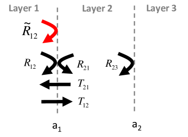
(a)

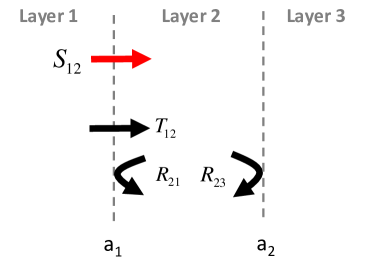
(b)

Figure 2: Schematic description of three layers with associated coefficients for the outgoing-potential case: (a) $R_{12}$ and (b) $S_{12}$.

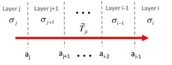
Figure 3: Generalized transmission coefficient for the outgoing-potential case.

For the standing-potential case depicted in Fig. 4, the potentials in three cylindrical layers can be written as

$$\psi_{1} =I_{n}(\lambda\rho)B_{1},$$ (13a)

$$\psi_{2} =\left[R_{21}K_{n}(\lambda\rho)+I_{n}(\lambda\rho)\right]B_{2},$$ (13b)

$$\psi_{3} =\left[\widetilde{R}_{32}K_{n}(\lambda\rho)+I_{n}(\lambda\rho)\right]B_{3}.$$ (13c)

Similarly, applying proper constraint conditions, we obtain

$$\widetilde{R}_{32}=R_{32}+T_{23}R_{21}(1-R_{23}R_{21})^{-1}T_{32}.$$ (14)

and, more generally,

$$\widetilde{R}_{i,i-1}=R_{i,i-1}+T_{i-1,i}\widetilde{R}_{i-1,i-2}(1-R_{i-1,i}\widetilde{R}_{i-1,i-2})^{-1}T_{i,i-1}.$$ (15)

To obtain all amplitudes $B_{i}$’s, it is convenient to define the $S$ coefficient with decreasing subscripts $S_{i,i-1}$. Since the relation between two successive amplitudes is

$$B_{i-1}=T_{i,i-1}B_{i}+R_{i-1,i}R_{i-1,i-2}B_{i-1},$$ (16)

the $S$ coefficient in this case is defined as

$$S_{i,i-1}=(1-R_{i-1,i}\widetilde{R}_{i-1,i-2})^{-1}T_{i,i-1}$$ (17)

such that $B_{i-1}=S_{i,i-1}B_{i}$. The generalized transmission coefficient depicted in Fig. 5 can then be written as

$$\widetilde{T}_{ji}=T_{i+1,i}S_{i+2,i+1}\cdots S_{j,j-1}=T_{i+1,i}\prod_{k=j}^{i+2}S_{k,k+1}=T_{i+1,i}X_{j,i+1}.$$ (18)

Note that $i<j$ for the outgoing-potential case. When $j=i+1$, $X_{j,i+1}=1$ in (18).

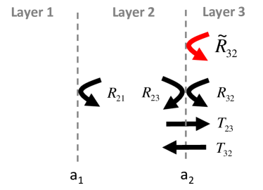
(a)

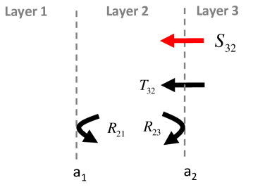
(b)

Figure 4: Schematic description of three layers with associated coefficients for the standing-potential case: (a) $R_{32}$ and (b) $S_{32}$.

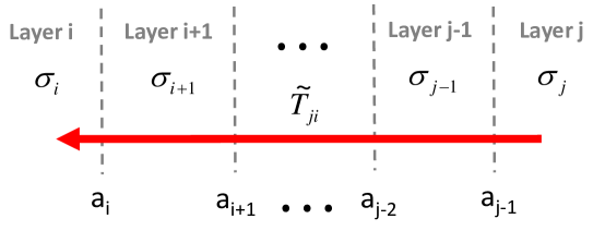
Figure 5: Generalized transmission coefficient for the standing-potential case.

Using generalized reflection and transmission coefficients, we can extend (2) to incorporate multiple reflections and transmissions. The integral part of (2) can be modified to

$$\int_{0}^{\infty}\left[I_{n}(\lambda\rho_{<})K_{n}(\lambda\rho_{>})+K_{n}(\lambda\rho)A_{jn}(\rho^{\prime})+I_{n}(\lambda\rho)B_{jn}(\rho^{\prime})\right]\cos(\lambda(z-z^{\prime}))d\lambda,$$ (19)

where the two unknowns are $A_{jn}(\rho^{\prime})$ and $B_{jn}(\rho^{\prime})$. Applying two constraint conditions at $\rho=a_{j-1}$ and $\rho=a_{j}$, we obtain

$$A_{jn}(\rho^{\prime})=(1-\widetilde{R}_{j,j-1}\widetilde{R}_{j,j+1})^{-1}\widetilde{R}_{j,j-1}\left[K_{n}(\lambda\rho^{\prime})+I_{n}(\lambda\rho^{\prime})\widetilde{R}_{j,j+1}\right],$$ (20a)

$$B_{jn}(\rho^{\prime})=(1-\widetilde{R}_{j,j+1}\widetilde{R}_{j,j-1})^{-1}\widetilde{R}_{j,j+1}\left[I_{n}(\lambda\rho^{\prime})+K_{n}(\lambda\rho^{\prime})\widetilde{R}_{j,j-1}\right].$$ (20b)

Substituting (20a) and (20b) into (19) and rearranging the integrand excluding the cosine factor gives

$$\left[I_{n}(\lambda\rho_{<})K_{n}(\lambda\rho_{>})+K_{n}(\lambda\rho)A_{jn}(\rho^{\prime})+I_{n}(\lambda\rho)B_{jn}(\rho^{\prime})\right]$$

$$=\left\{\begin{array}[]{l l}\left[K_{n}(\lambda\rho)+I_{n}(\lambda\rho)\widetilde{R}_{j,j+1}\right]\left[I_{n}(\lambda\rho^{\prime})+K_{n}(\lambda\rho^{\prime})\widetilde{R}_{j,j-1}\right]M_{j},&\quad\rho>\rho^{\prime}\\ \left[I_{n}(\lambda\rho)+K_{n}(\lambda\rho)\widetilde{R}_{j,j-1}\right]\left[K_{n}(\lambda\rho^{\prime})+I_{n}(\lambda\rho^{\prime})\widetilde{R}_{j,j+1}\right]M_{j},&\quad\rho<\rho^{\prime}\end{array}\right.$$ (23)

where $M_{j}=\left(1-\widetilde{R}_{j,j-1}\widetilde{R}_{j,j+1}\right)^{-1}$. When $i>j$, the potential in layer $i$ is expressed as

$$\psi_{i} =\frac{I}{2\pi^{2}\sigma_{j}}\sum_{n=-\infty}^{\infty}e^{\mathrm{i}n(\phi-\phi^{\prime})}\int_{0}^{\infty}\left[K_{n}(\lambda\rho)+I_{n}(\lambda\rho)\widetilde{R}_{i,i+1}\right]A_{in}\cos(\lambda(z-z^{\prime}))d\lambda,$$ (24)

where $A_{in}$ is the amplitude of the outgoing-potential in layer $i$ and expressed as

$$A_{in}=\left(1-R_{i,i-1}\widetilde{R}_{i,i+1}\right)\widetilde{T}_{ji}A_{jn}=N_{i+}\widetilde{T}_{ji}A_{jn}=N_{i+}\widetilde{T}_{ji}\left[I_{n}(\lambda\rho^{\prime})+K_{n}(\lambda\rho^{\prime})\widetilde{R}_{j,j-1}\right]M_{j}.$$ (25)

Therefore, the integrand factor for layer $i$ in (24) is

$$\left[K_{n}(\lambda\rho)+I_{n}(\lambda\rho)\widetilde{R}_{i,i+1}\right]\left[I_{n}(\lambda\rho^{\prime})+K_{n}(\lambda\rho^{\prime})\widetilde{R}_{j,j-1}\right]N_{i+}\widetilde{T}_{ji}M_{j}.$$ (26)

When $i<j$, the potential in layer $i$ is expressed as

$$\psi_{i} =\frac{I}{2\pi^{2}\sigma_{j}}\sum_{n=-\infty}^{\infty}e^{\mathrm{i}n(\phi-\phi^{\prime})}\int_{0}^{\infty}\left[I_{n}(\lambda\rho)+K_{n}(\lambda\rho)\widetilde{R}_{i,i-1}\right]A_{in}\cos(\lambda(z-z^{\prime}))d\lambda,$$ (27)

where $A_{in}$ is the amplitude of the standing-potential in layer $i$ and expressed as

$$A_{in}=\left(1-R_{i,i+1}\widetilde{R}_{i,i-1}\right)\widetilde{T}_{ji}A_{jn}=N_{i-}\widetilde{T}_{ji}A_{jn}\left[K_{n}(\lambda\rho^{\prime})+I_{n}(\lambda\rho^{\prime})\widetilde{R}_{j,j+1}\right]M_{j}$$ (28)

The integrand of the integral for potential in layer $i$ in (27) is

$$\left[I_{n}(\lambda\rho)+K_{n}(\lambda\rho)\widetilde{R}_{i,i-1}\right]\left[K_{n}(\lambda\rho^{\prime})+I_{n}(\lambda\rho^{\prime})\widetilde{R}_{j,j+1}\right]N_{i-}\widetilde{T}_{ji}M_{j}.$$ (29)

In summary, the potential in cylindrically stratified media admits four different expressions depending on the relative position of $\rho$ and $\rho^{\prime}$, which can be written as

$$\psi_{i} =\frac{\mathcal{I}}{2\pi^{2}\sigma_{j}}\sum_{n=-\infty}^{\infty}e^{\mathrm{i}n(\phi-\phi^{\prime})}\int_{0}^{\infty}F_{n}(\rho,\rho^{\prime})\cos(\lambda(z-z^{\prime}))d\lambda,$$ (30)

where

Case 1: $$\rho \rho^{\prime} \rho\geq\rho^{\prime}$$ and are in the same layer and

$$\quad F_{n}(\rho,\rho^{\prime})=\left[K_{n}(\lambda\rho)+I_{n}(\lambda\rho)\widetilde{R}_{j,j+1}\right]\left[I_{n}(\lambda\rho^{\prime})+K_{n}(\lambda\rho^{\prime})\widetilde{R}_{j,j-1}\right]M_{j},$$ (31a)

Case 2: $$\rho \rho^{\prime} \rho<\rho^{\prime}$$ and are in the same layer and

$$\quad F_{n}(\rho,\rho^{\prime})=\left[I_{n}(\lambda\rho)+K_{n}(\lambda\rho)\widetilde{R}_{j,j-1}\right]\left[K_{n}(\lambda\rho^{\prime})+I_{n}(\lambda\rho^{\prime})\widetilde{R}_{j,j+1}\right]M_{j},$$ (31b)

Case 3: $$\rho \rho^{\prime} \rho>\rho^{\prime}$$ and are in different layers and

$$\quad F_{n}(\rho,\rho^{\prime})=\left[K_{n}(\lambda\rho)+I_{n}(\lambda\rho)\widetilde{R}_{i,i+1}\right]\left[I_{n}(\lambda\rho^{\prime})+K_{n}(\lambda\rho^{\prime})\widetilde{R}_{j,j-1}\right]N_{i+}\widetilde{T}_{ji}M_{j},$$ (31c)

Case 4: $$\rho \rho^{\prime} \rho<\rho^{\prime}$$ and are in different layers and

$$\quad F_{n}(\rho,\rho^{\prime})=\left[I_{n}(\lambda\rho)+K_{n}(\lambda\rho)\widetilde{R}_{i,i-1}\right]\left[K_{n}(\lambda\rho^{\prime})+I_{n}(\lambda\rho^{\prime})\widetilde{R}_{j,j+1}\right]N_{i-}\widetilde{T}_{ji}M_{j}.$$ (31d)

2.3 Rescaled modified-Bessel functions

The electric potential involves products of the modified-Bessel function of the first and second kind, viz. $I_{n}$ and $K_{n}$. Those products can involve disparate values due to the exponential behavior of the functions. For example, when $|z|<<1$, $K_{n}(z)$ has very large value whereas $I_{n}(z)$ has very small value. This disparity becomes progressively worse for higher order modes. On the other hand, when $\Re e[z]>>1$, $K_{n}(z)$ has very small value while $I_{n}(z)$ has very large value. This leads to unreliable results under double-precision computations. To eliminate this problem, a new set of rescaled modified-Bessel functions are defined in a similar fashion to what has been done in [16] for Bessel and Hankel functions, viz. $J_{n}$ and $H^{(1)}_{n}$. In order to apply such rescaled functions, the analytical expressions for the potential need to modified accordingly, as described next.

When $|z|\ll 1$, $I_{n}(z)$ and $K_{n}(z)$ can be expressed via small argument approximations for $n>0$. Noting that, for $-\pi<arg(z)<\pi/2$, the relationship between cylindrical functions and modified-cylindrical functions reads as

$$I_{n}(z)=\mathrm{i}^{-n}J_{n}(iz),$$ (32a)

$$K_{n}(z)=\frac{\pi}{2}\mathrm{i}^{n+1}H^{(1)}_{n}(iz).$$ (32b)

Thus, we have the following small argument approximations for $I_{n}$ and $K_{n}$ and their derivatives.

$$I_{n}(\lambda a_{i}) \approx\frac{1}{n!}\left(\frac{\lambda a_{i}}{2}\right)^{n}=\frac{1}{n!}\left(\frac{\lambda}{2}\right)^{n}\cdot a_{i}^{n}\cdot 1=Ga_{i}^{n}\hat{I}_{n}(\lambda a_{i}),$$ (33a)

$$I^{\prime}_{n}(\lambda a_{i}) \approx\frac{1}{2(n-1)!}\left(\frac{\lambda a_{i}}{2}\right)^{n-1}=\frac{1}{n!}\left(\frac{\lambda}{2}\right)^{n}\cdot a_{i}^{n}\cdot\frac{n}{\lambda a_{i}}=Ga_{i}^{n}\hat{I}^{\prime}_{n}(\lambda a_{i}),$$ (33b)

$$K_{n}(\lambda a_{i}) \approx\frac{(n-1)!}{2}\left(\frac{2}{\lambda a_{i}}\right)^{n}=n!\left(\frac{2}{\lambda}\right)^{n}\cdot a_{i}^{-n}\cdot\left(\frac{1}{2n}\right)=G^{-1}a_{i}^{-n}\hat{K}_{n}(\lambda a_{i}),$$ (33c)

$$K^{\prime}_{n}(\lambda a_{i}) \approx-\frac{n!}{4}\left(\frac{2}{\lambda a_{i}}\right)^{n+1}=n!\left(\frac{2}{\lambda}\right)^{n}\cdot a_{i}^{-n}\cdot\left(-\frac{1}{2\lambda a_{i}}\right)=G^{-1}a_{i}^{-n}\hat{K}^{\prime}_{n}(\lambda a_{i}).$$ (33d)

It should be noted that the multiplicative factor $G$ above is chosen so as to not depend on the radial distance, $a_{i}$. Also, $G$ is identical for a function and its derivative, and the multiplicative factors appearing in $I_{n}$ and $K_{n}$ are reciprocal to each other. This will facilitate some computations later on.

When $\Re e[z]\gg 1$ and $z=\lambda a_{i}=(\lambda^{\prime}+\mathrm{i}\lambda^{\prime\prime})a_{i}$, the large argument approximations for the modified-Bessel functions write as [34]

$$I_{n}(\lambda a_{i}) =\frac{e^{\lambda a_{i}}}{\sqrt{2\pi\lambda a_{i}}}\left[1-\frac{(\mu-1)}{1!(8\lambda a_{i})}+\frac{(\mu-1)(\mu-9)}{2!(8\lambda a_{i})^{2}}+\dotsb\right]$$

$$=e^{\lambda^{\prime}a_{i}}\hat{I}_{n}(\lambda a_{i}),$$ (34a)

$$K_{n}(\lambda a_{i}) =\sqrt{\frac{\pi}{2\lambda a_{i}}}e^{-\lambda a_{i}}\left[1+\frac{(\mu-1)}{1!(8\lambda a_{i})}+\frac{(\mu-1)(\mu-9)}{2!(8\lambda a_{i})^{2}}+\dotsb\right]$$

$$=e^{-\lambda^{\prime}a_{i}}\hat{K}_{n}(\lambda a_{i}),$$ (34b)

where $\mu=4n^{2}$. Again, the associated multiplicative factors are reciprocal to each other. The derivatives of rescaled modified-cylindrical functions for large arguments can be derived through the recursive formulas such that

$$I^{\prime}_{n}(\lambda a_{i}) =I_{n-1}(\lambda a_{i})-\frac{n}{\lambda a_{i}}I_{n}(\lambda a_{i})=e^{\lambda^{\prime}a_{i}}\hat{I}_{n-1}(\lambda a_{i})-e^{\lambda^{\prime}a_{i}}\frac{n}{\lambda a_{i}}\hat{I}_{n}(\lambda a_{i})=e^{\lambda^{\prime}a_{i}}\hat{I}^{\prime}_{n}(\lambda a_{i}),$$ (35)

$$K^{\prime}_{n}(\lambda a_{i}) =-K_{n-1}(\lambda a_{i})-\frac{n}{\lambda a_{i}}K_{n}(\lambda a_{i})=-e^{-\lambda^{\prime}a_{i}}\hat{K}_{n-1}(\lambda a_{i})-e^{-\lambda^{\prime}a_{i}}\frac{n}{\lambda a_{i}}\hat{K}_{n}(\lambda a_{i})=e^{-\lambda^{\prime}a_{i}}\hat{K}^{\prime}_{n}(\lambda a_{i}).$$ (36)

If the argument is neither small nor large, rescaled modified-cylindrical functions are defined, in analogy to small and large arguments, as

$$I_{n}(\lambda a_{i}) =P_{i}\hat{I}_{n}(\lambda a_{i}),$$ (37a)

$$I^{\prime}_{n}(\lambda a_{i}) =P_{i}\hat{I}^{\prime}_{n}(\lambda a_{i}),$$ (37b)

$$K_{n}(\lambda a_{i}) =P_{i}^{-1}\hat{K}_{n}(\lambda a_{i}),$$ (37c)

$$K^{\prime}_{n}(\lambda a_{i}) =P_{i}^{-1}\hat{K}^{\prime}_{n}(\lambda a_{i}),$$ (37d)

where the multiplicative factor $P_{i}$ is defined as in [16], i.e.,

$$\text{If }|I_{n}(\lambda a_{i})|^{-1}<T_{m},\quad P_{i}=1.$$ (38a)

$$\text{If }|I_{n}(\lambda a_{i})|^{-1}\geq T_{m},\quad P_{i}=|I_{n}(\lambda a_{i})|.$$ (38b)

with $T_{m}=10^{1}00$ used for double-precision arithmetic computations.

and its subscript is linked to $a_{i}$. As Table 1 shows, the argument for rescaled modified-cylindrical functions can be categorized into small, moderate, and large, with different and appropriate multiplicative factors defined accordingly.

Table 1: Definition of rescaled modified-cylindrical functions for all types of arguments.

	small arguments	moderate arguments	large arguments
$I_{n}(\lambda a_{i})$	$Ga_{i}^{n}\hat{I}_{n}(\lambda a_{i})$	$P_{i}\hat{I}_{n}(\lambda a_{i})$	$e^{\lambda^{\prime}a_{i}}\hat{I}_{n}(\lambda a_{i})$
$I^{\prime}_{n}(\lambda a_{i})$	$Ga_{i}^{n}\hat{I}^{\prime}_{n}(\lambda a_{i})$	$P_{i}\hat{I}^{\prime}_{n}(\lambda a_{i})$	$e^{\lambda^{\prime}a_{i}}\hat{I}^{\prime}_{n}(\lambda a_{i})$
$K_{n}(\lambda a_{i})$	$G^{-1}a_{i}^{-n}\hat{K}_{n}(\lambda a_{i})$	$P_{i}^{-1}\hat{K}_{n}(\lambda a_{i})$	$e^{-\lambda^{\prime}a_{i}}\hat{K}_{n}(\lambda a_{i})$
$K^{\prime}_{n}(\lambda a_{i})$	$G^{-1}a_{i}^{-n}\hat{K}^{\prime}_{n}(\lambda a_{i})$	$P_{i}^{-1}\hat{K}^{\prime}_{n}(\lambda a_{i})$	$e^{-\lambda^{\prime}a_{i}}\hat{K}^{\prime}_{n}(\lambda a_{i})$

The numerical threshold values used here to define small, moderate, and large argument ranges are identical to those used for the time-harmonic case involving cylindrical Bessel and Hankel functions detailed in [16] and not repeated here.

2.4 Rescaled reflection and transmission coefficients

We can classify the multiplicative factors associated with the rescaled modified-cylindrical functions into two types, denoted as $\alpha$ and $\beta$, and shown in Table 2. The factor $\alpha_{i}$ is associated with $K_{n}(\lambda a_{i})$, whereas $\beta_{i}$ is associated with $I_{n}(\lambda a_{i})$. Note again that the subscript $i$ refers to to the index of the radial factor $a_{i}$ in the argument. There are two important properties to note for $\alpha$ and $\beta$: ($i$)Reciprocity: $\alpha_{i}=1/\beta_{i}$ and ($ii$) Boundness: $|\beta_{i}\alpha_{j}|\leq 1,\quad\text{for }i<j$. As we will see below, these two properties are important in ensuring stable numerical computations.

Table 2: Definition of $\alpha_{i}$ and $\beta_{i}$.

argument type	$\alpha_{i}$	$\beta_{i}$
small	$G^{-1}a^{-n}_{i}$	$Ga^{n}_{i}$
moderate	$P_{i}^{-1}$	$P_{i}$
large	$e^{-\lambda^{\prime}a_{i}}$	$e^{\lambda^{\prime}a_{i}}$

Recalling the expressions for the reflection and transmission coefficients obtained before, the reflection coefficient $R_{12}$ for the outgoing-potential case is modified to

$$R_{12} =\frac{(\sigma_{2}-\sigma_{1})K_{n}(\lambda a_{1})K^{\prime}_{n}(\lambda a_{1})}{\sigma_{1}I^{\prime}_{n}(\lambda a_{1})K_{n}(\lambda a_{1})-\sigma_{2}I_{n}(\lambda a_{1})K^{\prime}_{n}(\lambda a_{1})}$$

$$=\alpha_{1}^{2}\frac{(\sigma_{2}-\sigma_{1})\hat{K}_{n}(\lambda a_{1})\hat{K}^{\prime}_{n}(\lambda a_{1})}{\sigma_{1}\hat{I}^{\prime}_{n}(\lambda a_{1})\hat{K}_{n}(\lambda a_{1})-\sigma_{2}\hat{I}_{n}(\lambda a_{1})\hat{K}^{\prime}_{n}(\lambda a_{1})}$$

$$=\alpha_{1}^{2}\hat{R}_{12}.$$ (39)

Similarly, it can be shown that the reflection coefficient $R_{21}$ for the standing-potential case is modified to $R_{21}=\beta_{1}^{2}\hat{R}_{21}$, and that the transmission coefficient $T_{12}$ for the outgoing-potential case and the transmission coefficient $T_{21}$ for the standing-potential case simply recover the original ones without any multiplicative factors, i.e. $T_{12}=\hat{T}_{12}$ and $T_{21}=\hat{T}_{21}$.

Based on the above modifications for the reflection and transmission coefficients, generalized reflection and transmission coefficients for thre or more layers can be similarly modified. After some algebra, it can be shown that $\widetilde{R}_{i,i+1}=\alpha_{i}^{2}\hat{\widetilde{R}}_{i,i+1}$ and $\widetilde{R}_{i+1,i}=\beta_{i}^{2}\hat{\widetilde{R}}_{i+1,i}$, and that, for both the outgoing-potential and standing-potential cases, $\widetilde{T}_{ij}=\hat{\widetilde{T}}_{ij}$.

In addition to generalized reflection and transmission coefficients, the factors $M_{j}$ and $N_{i\pm}$ considered before are also required to compute the potential. The basic difference between the two types of coefficients is that $M_{j}$ involves two generalized reflection coefficients whereas $N_{i\pm}$ involves only one generalized reflection coefficient. All these auxiliary coefficients can be redefined accordingly using rescaled reflection coefficients, i.e.,

$$M_{j} =\left[1-\widetilde{R}_{j,j-1}\widetilde{R}_{j,j+1}\right]^{-1}=\left[1-\beta^{2}_{j-1}\alpha^{2}_{j}\hat{\widetilde{R}}_{j,j-1}\hat{\widetilde{R}}_{j,j+1}\right]^{-1},$$ (40a)

$$N_{i+} =\left[1-R_{i,i-1}\widetilde{R}_{i,i+1}\right]^{-1}=\left[1-\beta^{2}_{i-1}\alpha^{2}_{i}\hat{R}_{i,i-1}\hat{\widetilde{R}}_{i,i+1}\right]^{-1},$$ (40b)

$$N_{i-} =\left[1-R_{i,i+1}\widetilde{R}_{i,i-1}\right]^{-1}=\left[1-\beta^{2}_{i-1}\alpha^{2}_{i}\hat{R}_{i,i+1}\hat{\widetilde{R}}_{i,i-1}\right]^{-1}.$$ (40c)

2.5 Rescaled integrand

Nest step is to modify the full integrand using rescaled modified-cylindrical functions. Since there are four integrand expressions, depending of the relative position of $\rho$ and $\rho^{\prime}$, each case is considered separately.

For Case 1, there are four radial parameters of interest: $a_{j-1}$, $\rho^{\prime}$, $\rho$, and $a_{j}$. For convenience, we let $a_{j-1}=a_{1}$, $\rho^{\prime}=a_{2}$, $\rho=a_{3}$, and $a_{j}=a_{4}$ so that $a_{1}<a_{2}<a_{3}<a_{4}$, and the integrand rewrites as

$$F_{n}(\rho,\rho^{\prime}) =\left[K_{n}(\lambda\rho)+I_{n}(\lambda\rho)\widetilde{R}_{j,j+1}\right]\left[I_{n}(\lambda\rho^{\prime})+K_{n}(\lambda\rho^{\prime})\widetilde{R}_{j,j-1}\right]M_{j}$$

$$=\left[\beta_{2}\alpha_{3}\hat{K}_{n}(\lambda\rho)+(\beta_{2}\alpha_{4})(\beta_{3}\alpha_{4})\hat{I}_{n}(\lambda\rho)\hat{\widetilde{R}}_{j,j+1}\right]\left[\hat{I}_{n}(\lambda\rho^{\prime})+(\beta_{1}\alpha_{2})^{2}\hat{K}_{n}(\lambda\rho^{\prime})\hat{\widetilde{R}}_{j,j-1}\right]M_{j}$$

$$=\left[A_{1}\hat{K}_{n}(\lambda\rho)+A_{2}\hat{I}_{n}(\lambda\rho)\hat{\widetilde{R}}_{j,j+1}\right]\left[A_{3}\hat{I}_{n}(\lambda\rho^{\prime})+A_{4}\hat{K}_{n}(\lambda\rho^{\prime})\hat{\widetilde{R}}_{j,j-1}\right]M_{j},$$ (41)

where $\beta_{2}^{-1}=\alpha_{2}$ has been used. All multiplicative factors $A_{1}$, $A_{2}$, $A_{3}$, $A_{4}$ have magnitudes no larger than one due to the boundness property discussed above.

Similarly, for Case 2, there are four radial parameters of interest: $a_{j-1}$, $\rho$, $\rho^{\prime}$, and $a_{j}$. For convenience, we let $a_{j-1}=a_{1}$, $\rho=a_{2}$, $\rho^{\prime}=a_{3}$, and $a_{j}=a_{4}$ so that $a_{1}<a_{2}<a_{3}<a_{4}$, and the integrand rewrites as

$$F_{n}(\rho,\rho^{\prime}) =\left[I_{n}(\lambda\rho)+K_{n}(\lambda\rho)\widetilde{R}_{j,j-1}\right]\left[K_{n}(\lambda\rho^{\prime})+I_{n}(\lambda\rho^{\prime})\widetilde{R}_{j,j+1}\right]M_{j}$$

$$=\left[\beta_{2}\alpha_{3}\hat{I}_{n}(\lambda\rho)+(\beta_{1}\alpha_{2})(\beta_{1}\alpha_{3})\hat{K}_{n}(\lambda\rho)\hat{\widetilde{R}}_{j,j-1}\right]\left[\hat{K}_{n}(\lambda\rho^{\prime})+(\beta_{3}\alpha_{4})^{2}\hat{I}_{n}(\lambda\rho^{\prime})\hat{\widetilde{R}}_{j,j+1}\right]M_{j}$$

$$=\left[B_{1}\hat{I}_{n}(\lambda\rho)+B_{2}\hat{K}_{n}(\lambda\rho)\hat{\widetilde{R}}_{j,j-1}\right]\left[B_{3}\hat{K}_{n}(\lambda\rho^{\prime})+B_{4}\hat{I}_{n}(\lambda\rho^{\prime})\hat{\widetilde{R}}_{j,j+1}\right]M_{j}.$$ (42)

Again, all multiplicative factors $B_{1}$, $B_{2}$, $B_{3}$, $B_{4}$ magnitudes are bounded by one.

For Case 3, there are six radial parameters of interest: $a_{j-1}$, $\rho^{\prime}$, $a_{j}$, $a_{i-1}$, $\rho$, and $a_{i}$. For convenience, we let $a_{j-1}=a_{1}$, $\rho^{\prime}=a_{2}$, $a_{j}=a_{3}$, $a_{i-1}=a_{4}$, $\rho=a_{5}$, and $a_{i}=a_{6}$ so that so that $a_{1}<a_{2}<a_{3}\leq a_{4}<a_{5}<a_{6}$, and the integrand rewrites as

$$F_{n}(\rho,\rho^{\prime}) =\left[K_{n}(\lambda\rho)+I_{n}(\lambda\rho)\widetilde{R}_{i,i+1}\right]\left[I_{n}(\lambda\rho^{\prime})+K_{n}(\lambda\rho^{\prime})\widetilde{R}_{j,j-1}\right]N_{i+}\widetilde{T}_{ji}M_{j}$$

$$=\left[\beta_{2}\alpha_{5}\hat{K}_{n}(\lambda\rho)+(\beta_{2}\alpha_{6})(\beta_{5}\alpha_{6})\hat{I}_{n}(\lambda\rho)\hat{\widetilde{R}}_{i,i+1}\right]\left[\hat{I}_{n}(\lambda\rho^{\prime})+(\beta_{1}\alpha_{2})^{2}\hat{K}_{n}(\lambda\rho^{\prime})\hat{\widetilde{R}}_{j,j-1}\right]N_{i+}\widetilde{T}_{ji}M_{j}$$

$$=\left[C_{1}\hat{K}_{n}(\lambda\rho)+C_{2}\hat{I}_{n}(\lambda\rho)\hat{\widetilde{R}}_{i,i+1}\right]\left[C_{3}\hat{I}_{n}(\lambda\rho^{\prime})+C_{4}\hat{K}_{n}(\lambda\rho^{\prime})\hat{\widetilde{R}}_{j,j-1}\right]N_{i+}\widetilde{T}_{ji}M_{j}.$$ (43)

All multiplicative factors $C_{1}$, $C_{2}$, $C_{3}$, $C_{4}$ have magnitudes never greater than unity.

Finally, for Case 4, there are again six radial parameters of interest: $a_{i-1}$, $\rho$, $a_{i}$, $a_{j-1}$, $\rho^{\prime}$, and $a_{j}$. For convenience, we let $a_{i-1}=a_{1}$, $\rho=a_{2}$, $a_{i}=a_{3}$, $a_{j-1}=a_{4}$, $\rho^{\prime}=a_{5}$, and $a_{j}=a_{6}$ so that $a_{1}<a_{2}<a_{3}\leq a_{4}<a_{5}<a_{6}$, and the integrand rewrites as

$$F_{n}(\rho,\rho^{\prime}) =\left[I_{n}(\lambda\rho)+K_{n}(\lambda\rho)\widetilde{R}_{i,i-1}\right]\left[K_{n}(\lambda\rho^{\prime})+I_{n}(\lambda\rho^{\prime})\widetilde{R}_{j,j+1}\right]N_{i-}\widetilde{T}_{ji}M_{j}$$

$$=\left[\beta_{2}\alpha_{5}\hat{I}_{n}(\lambda\rho)+(\beta_{1}\alpha_{2})(\beta_{1}\alpha_{5})\hat{K}_{n}(\lambda\rho)\hat{\widetilde{R}}_{i,i-1}\right]\left[\hat{K}_{n}(\lambda\rho^{\prime})+(\beta_{5}\alpha_{6})^{2}\hat{I}_{n}(\lambda\rho^{\prime})\hat{\widetilde{R}}_{j,j+1}\right]N_{i-}\widetilde{T}_{ji}M_{j}$$

$$=\left[D_{1}\hat{I}_{n}(\lambda\rho)+D_{2}\hat{K}_{n}(\lambda\rho)\hat{\widetilde{R}}_{i,i-1}\right]\left[D_{3}\hat{K}_{n}(\lambda\rho^{\prime})+D_{4}\hat{I}_{n}(\lambda\rho^{\prime})\hat{\widetilde{R}}_{j,j+1}\right]N_{i-}\widetilde{T}_{ji}M_{j}.$$ (44)

Once more, all multiplicative factors $D_{1}$, $D_{2}$, $D_{3}$, $D_{4}$ have magnitudes never greater than one.

2.6 Numerical integration

The electric potential expression includes a semi-infinite integral and an infinite series summation, as shown in (30). Therefore, truncation errors are inevitable and an error analysis should be made to ensure reliable results. In addition, the involved Sommerfeld-type integrals can be notoriously slowly convergent. A variety of extrapolation methods are applied here in order to accelerate the numerical integration, as described in more detail in Appendix B.

3 Results

A number of cases of practical interest for geophysical exploration are considered next. The results below are obtained on 2.6 GHz Opteron with 8 cores and 32 GB memory. For all cases below, the relative permittivity $\epsilon_{r}$ and relative permeability $\mu_{r}$ are set to one. The innermost layer has $6^{\prime\prime}$ radius and represents a mud-filled borehole. The outer layers represent the adjacent Earth formations, invasion zones, and/or casing layers. Each layer assumes different resistivity values $\mathcal{R}$, where $\mathcal{R}=1/\sigma$. As Fig. 6 illustrates, a current source emitting a DC current of 1 A is located at the Survey Electrode position. The electric potential is measured at two points: the Measurement Electrode 1 ($V_{16^{\prime\prime}}$) positioned 16 inches away from the source along the vertical direction and the Measurement Electrode 2 ($V_{32^{\prime\prime}}$) positioned 32 inches away from the source along the vertical direction. Both the source and two measurement electrodes are spaced 5 inches away from the $z$-axis and their azimuthal positions are the same ($\phi=\phi^{\prime}=0$). The relevant error parameters as defined in the Appendix and used in the following are $e_{tol}=10^{-4}$ and $e_{thr}=10^{-4}$. The electric potential and resistivity units used here are $[V]$ and $[\Omega\cdot m]$, respectively. The results of the present algorithm are compared against those from the finite element method (FEM).

3.1 Logging simulation results

Case 1 corresponds to a homogeneous problem, where analytical solutions are available. As Table 3 shows, the new algorithm produces very accurate results with very fast computing time. This is very important for making feasible the solution of the inverse problem (i.e., determining the unknown resistivity profile from known electric potential at the received electrodes) using iterative methods predicated on repeated forward solves.

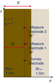
Figure 6: Case 1 in the $\rho z$-plane with $\mathcal{R}_{1}=\mathcal{R}_{2}=1$.

Table 3: Comparison of electric potential for Case 1.

	Analytical	FEM	Present Algorithm
$V_{16^{\prime\prime}}$	1.9581 $\times\;10^{-1}$	1.7878 $\times\;10^{-1}$	1.9580 $\times\;10^{-1}$ (2 sec.)
$V_{32^{\prime\prime}}$	9.7905 $\times\;10^{-2}$	9.4416 $\times\;10^{-2}$	9.7900 $\times\;10^{-2}$ (2 sec.)
$\Delta V$	9.7905 $\times\;10^{-2}$	8.4371 $\times\;10^{-2}$	9.7902 $\times\;10^{-2}$

Cases 2 and 3 correspond to a two-layer problem with 1:5 contrast between the adjacent borehole and formation resistivities.

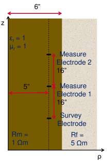
(a)

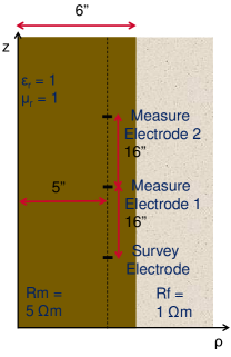
(b)

Figure 7: Cases 2 and 3 in the $\rho z$-plane: (a) Case 2 with $\mathcal{R}_{1}=1$, $\mathcal{R}_{2}=5$ and (b) Case 3 with $\mathcal{R}_{1}=5$, $\mathcal{R}_{2}=1$.

Table 4: Comparison of electric potential for Case 2.

	FEM	Present Algorithm
$V_{16^{\prime\prime}}$	9.5544 $\times\;10^{-1}$	9.7802 $\times\;10^{-1}$ (2 sec.)
$V_{32^{\prime\prime}}$	5.4241 $\times\;10^{-1}$	5.4981 $\times\;10^{-1}$ (2 sec.)
$\Delta V$	4.1303 $\times\;10^{-1}$	4.2822 $\times\;10^{-1}$

Table 5: Comparison of electric potential for Case 3.

	FEM	Present Algorithm
$V_{16^{\prime\prime}}$	1.6945 $\times\;10^{-1}$	2.0533 $\times\;10^{-1}$ (2 sec.)
$V_{32^{\prime\prime}}$	9.0310 $\times\;10^{-2}$	9.7677 $\times\;10^{-2}$ (2 sec.)
$\Delta V$	7.9145 $\times\;10^{-2}$	1.0766 $\times\;10^{-1}$

Cases 4 and 5 include a highly conductive casing. As Table 7 shows, there is disagreement between the semi-analytical and FEM results w.r.t. the absolute value of the electric potentials, although the computed potential differences (voltage drop) between the two electrodes are very similar. This disagreement is easy to explain as a FEM mesh truncation effect. The electric current in this case flows primarily along the thin, highly conductive casing, which does not produce sufficient decay on the electric potential before before it reaches the mesh boundary. Consequently, the FEM result has a spurious potential offset. The FEM has difficulty in simulating this problem unless a mesh truncation treatment is included on both top and bottom boundaries and/or a very long mesh is used along the $z$ direction. Notwithstanding such discrepancy, note that, in a resistivity logging context, the primary quantity of interest is the potential difference between electrodes.

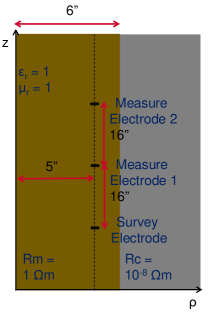
(a)

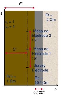
(b)

Figure 8: Cases 4 and 5 in the $\rho z$-plane: (a) Case 4 with $\mathcal{R}_{1}=1$, $\mathcal{R}_{2}=10^{-8}$ and (b) Case 5 with $\mathcal{R}_{1}=1$, $\mathcal{R}_{2}=10^{-8}$, $R_{3}=2$.

Table 6: Comparison of electric potential for Case 4.

	FEM	Present Algorithm
$V_{16^{\prime\prime}}$	1.2980 $\times\;10^{-4}$	1.3873 $\times\;10^{-4}$ (2 sec.)
$V_{32^{\prime\prime}}$	2.1372 $\times\;10^{-7}$	2.1415 $\times\;10^{-7}$ (2 sec.)
$\Delta V$	1.2959 $\times\;10^{-4}$	1.3852 $\times\;10^{-4}$

Table 7: Comparison of electric potential for Case 5.

	FEM	Present Algorithm
$V_{16^{\prime\prime}}$	2.2658 $\times\;10^{-4}$	1.7241 $\times\;10^{-3}$ (3 sec.)
$V_{32^{\prime\prime}}$	9.6331 $\times\;10^{-5}$	1.5885 $\times\;10^{-3}$ (2 sec.)
$\Delta V$	1.3025 $\times\;10^{-4}$	1.3562 $\times\;10^{-4}$

As Fig. 9 illustrates, Cases 6 and 7 feature two layers besides the borehole, where the mud layer can represent an invasion zone with a resistivity between those of the borehole and the outer formation.

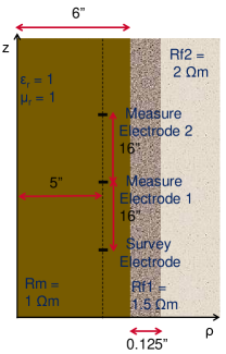
(a)

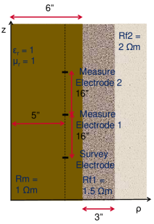
(b)

Figure 9: Cases 6 and 7 in the $\rho z$-plane: (a) Case 6 with $\mathcal{R}_{1}=1$, $\mathcal{R}_{2}=1.5$, $\mathcal{R}_{3}=2$ and (b) Case 7 with $\mathcal{R}_{1}=1$, $\mathcal{R}_{2}=1.5$, $\mathcal{R}_{3}=2$.

Table 8: Comparison of electric potential for Case 6.

	FEM	Present Algorithm
$V_{16^{\prime\prime}}$	3.7097 $\times\;10^{-1}$	3.9061 $\times\;10^{-1}$ (2 sec.)
$V_{32^{\prime\prime}}$	1.9796 $\times\;10^{-1}$	2.0245 $\times\;10^{-1}$ (2 sec.)
$\Delta V$	1.7301 $\times\;10^{-1}$	1.8816 $\times\;10^{-1}$

Table 9: Comparison of electric potential for Case 7.

	FEM	Present Algorithm
$V_{16^{\prime\prime}}$	3.6077 $\times\;10^{-1}$	3.8160 $\times\;10^{-1}$ (2 sec.)
$V_{32^{\prime\prime}}$	1.9694 $\times\;10^{-1}$	2.0156 $\times\;10^{-1}$ (2 sec.)
$\Delta V$	1.6383 $\times\;10^{-1}$	1.8003 $\times\;10^{-1}$

3.2 Electric potential maps

Plots of the spatial distributions of the electric potential of Cases 2–5 are provided next. Since the potential varies by many orders of magnitude near the electrodes, a log-scale is used; i.e. we plot the quantity $10\log_{10}|V|$. Fig. 10 depicts the potential distributions using a three-dimensional view. Fig. 11 and Fig. 12 show the cross-sections of the potential distributions at the $z=16^{\prime\prime}$ and $z=32^{\prime\prime}$ planes, respectively, while Fig. 13 shows the cross-sections at the $y=0^{\prime\prime}$ plane. In all figures, thicker black lines represent interfaces between cylindrical layers and thinner black lines represent equipotential contours. Note that the third layer of Case 5 is too thin for visualization in these plots.

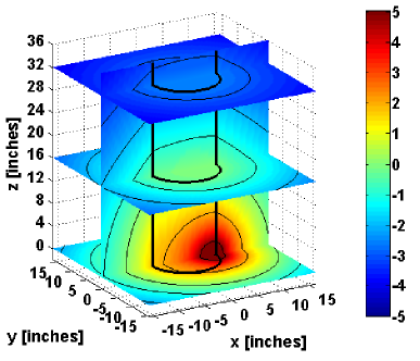
(a)

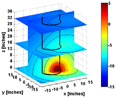
(b)

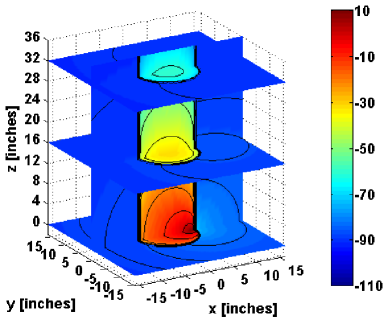
(c)

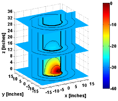
(d)

Figure 10: Electric potential around the current electrode: (a) Case 2, (b) Case 3, (c) Case 4, and (d) Case 5.

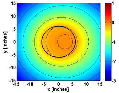
(a)

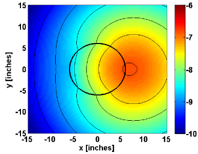
(b)

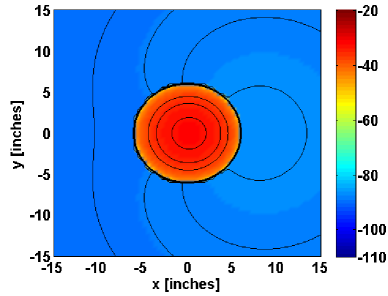
(c)

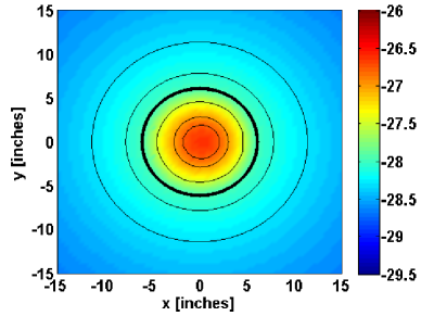
(d)

Figure 11: Electric potential at $z=16^{\prime\prime}$ plane around the current electrode: (a) Case 2, (b) Case 3, (c) Case 4, and (d) Case 5.

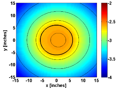
(a)

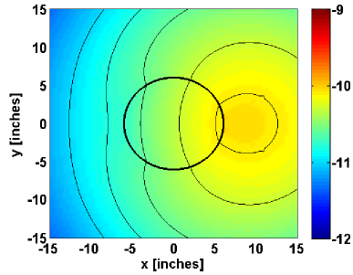
(b)

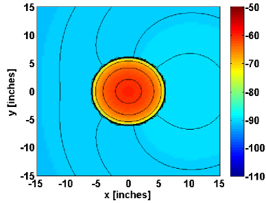
(c)

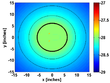
(d)

Figure 12: Electric potential at $z=32^{\prime\prime}$ plane around the current electrode: (a) Case 2, (b) Case 3, (c) Case 4, and (d) Case 5.

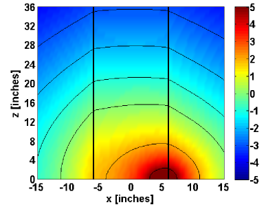
(a)

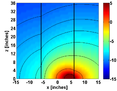
(b)

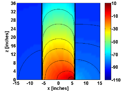
(c)

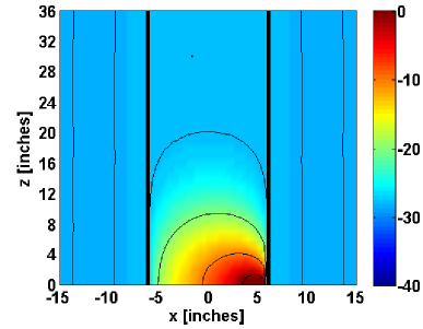
(d)

Figure 13: Electric potential at $y=0^{\prime\prime}$ plane around the current electrode: (a) Case 2, (b) Case 3, (c) Case 4, and (d) Case 5.

4 Conclusion

We have introduced a stable semianalytical formulation to compute the potential due to arbitrary-located electrodes in a cylindrically layered media, where the physical parameters (viz., layer resistivity) can vary by many order of magnitude. Stability was achieved by a rescaling of the modified Bessel functions and subsequent manipulation of the integrand expressions to avoid underflow and overflow problems under double-precision arithmetic. Several extrapolation methods to compute the involved Sommerfeld integrals were also considered and evaluated. The resulting algorithm was verified in a number of cases relevant to borehole geophysics. The fast speed and robustness of the algorithm makes it also quite suited as a forward solver engine for the inverse roblem, where the formation resistivity needs to be estimated from a limited numberof computed (measured) potential data. The same basic algorithm can be applied to other steady-state diffusion problems obeying Poisson’s equation with discontinous coefficients in cylindrically layered geometries.

Appendix A: Folding azimuth summation

The computation of potential in (30) involves infinite series over the azimuth mode $n$. For an arbitrary order $\nu\geq 0$ [34], we have

$$I_{-\nu}(z) =I_{\nu}(z)+\frac{2}{\pi}\sin(\nu\pi)K_{\nu}(z),$$ (45a)

$$K_{-\nu}(z) =K_{\nu}(z).$$ (45b)

If the order is a positive integer, $\nu=n$, the above reduces to $I_{-n}(z)=I_{n}(z)$ and $K_{-n}(z)=K_{n}(z)$. Consequently, we can write

$$\psi_{i} =\frac{\mathcal{I}}{2\pi^{2}\sigma_{j}}\sum_{n=-\infty}^{\infty}e^{\mathrm{i}n(\phi-\phi^{\prime})}\int_{0}^{\infty}F_{n}(\rho,\rho^{\prime})\cos(\lambda(z-z^{\prime}))d\lambda$$

$$=\frac{\mathcal{I}}{2\pi^{2}\sigma_{j}}\int_{0}^{\infty}\left[F_{0}(\rho,\rho^{\prime})+2\sum_{n=1}^{\infty}F_{n}(\rho,\rho^{\prime})\cos(n(\phi-\phi^{\prime}))\right]\cos(\lambda(z-z^{\prime}))d\lambda.$$ (46)

Appendix B: Extrapolation methods and convergence study

Among numerous extrapolation methods, some popular ones for Sommerfeld-type integrals are very briefly revisited here. For more details, the reader can refer, e.g., to [15, 33]. Before a given sequence is extrapolated, a Sommerfeld-type integral can be divided into a number of subintervals as

$$S=\int_{a}^{\infty}g(\lambda)p(\lambda)d\lambda=\sum_{i=0}^{\infty}\int_{\lambda_{i-1}}^{\lambda_{i}}g(\lambda)p(\lambda)d\lambda=\sum_{i=0}^{\infty}u_{i},$$ (47)

where $g(\lambda)$ is an exponentially decaying part and $p(\lambda)$ is an oscillatory part. This is called the partition-extrapolation approach [28]. In general, the remainders are defined as

$$r_{n}=S_{n}-S=-\int_{\lambda_{n}}^{\infty}g(\lambda)p(\lambda)d\lambda.$$ (48)

Furthermore, the remainders are assumed to feature Poincaré-type asymptotic expansions [15] of the form

$$r_{n}\sim\omega_{n}\sum_{i=0}^{\infty}a_{i}\lambda^{-i}_{n},\qquad n\rightarrow\infty,$$ (49)

where $\omega_{n}$ is the remainder estimate and $a_{i}$ are associated coefficients. The estimates $\omega_{n}$ play an important role in the extrapolation and can be obtained analytically or numerically. The coefficients $a_{i}$ are unknowns but they are not necessary for the extrapolation itself. In our case, $g(\lambda)$ in (47) can be asymptotically expressed as

$$g(\lambda)\sim\frac{e^{-\lambda|\rho-\rho^{\prime}|}}{\lambda}\sum_{i=0}^{\infty}\frac{c_{i}}{\lambda^{i}},$$ (50)

where $c_{i}$ are arbitrary constants. Furthermore, $p(\lambda)=\cos(\lambda(z-z^{\prime}))$ with half-period equal to $\pi/|\rho-\rho^{\prime}|$. After some algebra, it can be shown that the remainder estimates write as

$$\omega_{n}=\frac{(-1)^{n+1}}{\lambda_{n}}e^{-\frac{n\pi|\rho-\rho^{\prime}|}{|z-z^{\prime}|}}.$$ (51)

We list next three popular extrapolation methods for a given sequence, $\{S_{n}\}=S_{0},S_{1},S_{2},\cdots,S_{n}$, where we consider $S_{n}=S_{n}^{(0)}$.

(i) Euler transformation

$$S_{n}^{(k+1)}=\frac{1}{2}\left(S_{n}^{(k)}+S_{n+1}^{(k)}\right),\qquad n,k\geq 0$$ (52)

The best approximation in this case is $S_{0}^{(k)}|_{k=n}$, and this choice is most effective for logarithmic alternating sequences.

(ii) Iterative Aitken transformation

$$S_{n}^{(k+1)}=S_{n}^{(k)}-\frac{[\Delta S_{n}^{(k)}]^{2}}{\Delta^{2}S_{n}^{(k)}},\qquad n,k\geq 0$$ (53)

Note that $\Delta S^{(k)}_{n}=S_{n+1}^{(k)}-S_{n}^{(k)}$ and $\Delta^{2}S_{n}^{(k)}=S_{n+2}^{(k)}-2S_{n+1}^{(k)}+S_{n}^{(k)}$. Obviously, this is a nonlinear transformation and it can be applied to both linear monotone and alternating sequences. When an odd number of sequences is given, the best approximation is $S_{0}^{(k)}|_{k=n}$. For an even number, the best approximation is $S_{1}^{(k)}|_{k=n}$.

(iii) Weighted-averages method

$$S^{(k+1)}_{n}=\frac{S^{(k)}_{n}+\eta^{(k)}_{n}S^{(k)}_{n+1}}{1+\eta^{(k)}_{n}},\qquad n,k\geq 0,$$ (54)

where $\eta^{(k)}$ is the weight and defined as

$$\eta^{(k)}=-\frac{\omega_{n}}{\omega_{n+1}}=\frac{\lambda_{n+1}}{\lambda_{n}}e^{\frac{\pi|\rho-\rho^{\prime}|}{|z-z^{\prime}|}}.$$ (55)

The weighted-averages method [18, 19] can be regarded as generalized Euler transformation since $\eta=1$ recovers the Euler transformation. The relative power of this method, compared to the two other methods, comes from using remainder estimates. As pointed out in [15], the weighted-averages method is quited suited for extrapolating Sommerfeld-type integrals.

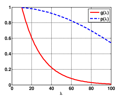
(a)

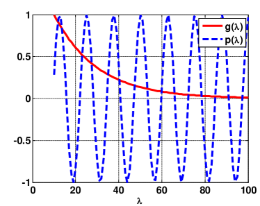
(b)

Figure 14: Two scenarios of the integrand: (a) Type 1 with $|\rho-\rho^{\prime}|=0.05$, $|z-z^{\prime}|=0.01$ and (b) Type 2 with $|\rho-\rho^{\prime}|=0.05$, $|z-z^{\prime}|=0.5$.

To evaluate the integral (47), the subinterval length $q$ should be first determined. As suggested in [15], the half-period of the oscillating part of the integrand is a good choice for $q$ because it makes the sequences alternating; i.e., $q=\pi/|z-z^{\prime}|$. However, this is not appropriate here in some circumstances. Let us consider the two scenarios depicted in Fig. 14. The two figures show the behavior of $g(\lambda)$ and $p(\lambda)$ for different combinations of $|\rho-\rho^{\prime}|$ and $|z-z^{\prime}|$ as $\lambda$ increases. For better visualization, the functions are normalized by their respective maxima. Type 1 integrand occurs when $|\rho-\rho^{\prime}|>|z-z^{\prime}|$ and shows linear monotone convergence. On the other hand, Type 2 integrand occurs when $|\rho-\rho^{\prime}|<|z-z^{\prime}|$ and shows logarithmic alternating convergence. Therefore, such an expression for $q$ is not appropriate for Type 1 because the integrand is near zero before the first half-period comes. For the Type 1 integrand, a different subinterval length can be defined as $q=\pi/|\rho-\rho^{\prime}|$, so that the subinterval length can be written in general as

$$q=\frac{\pi}{\text{max}(|\rho-\rho^{\prime}|,|z-z^{\prime}|)}.$$ (56)

Once $q$ is determined, it becomes necessary to determine how many subintervals are required to reach sufficient convergence. To do so, the relative error below is defined

$$e_{i}=\frac{|T(S_{i+1})-T(S_{i})|}{|T(S_{i+1})|},$$ (57)

where $T(S_{i})$ is the extrapolated (transformed) value for given sequences, $\{S_{i}\}=S_{0},S_{1},\cdots,S_{i}$. If $e_{i}$ is less than a given error tolerance $e_{tol}$, the sequence is stopped and the number of subintervals is determined. Next, the number of quadrature points per the subinterval is increased until the relative error between two adjacent iterations meets the desired criterion. To distinguish it from $e_{tol}$, the criterion in this step is denoted error threshold $e_{thr}$. The same step is repeated for determining the number of orders. The overall procedure is schematically depicted in Fig. 15.

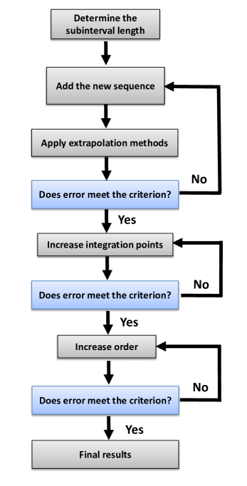
Figure 15: Flowchart of the procedure for computation of electric potential using extrapolation methods.

Some convergence tests are performed next to evaluate the numerical integration procedures above. The domain is assumed homogeneous because exact (analytical) solutions are available as reference. Three cases of source/observation distances are considered.

Case 1 : $\;|\rho-\rho^{\prime}|=0.001\text{ m}$, $\;|z-z^{\prime}|=0.1\text{ m}$

Case 2 : $\;|\rho-\rho^{\prime}|=\quad 0.1\text{ m}$, $\;|z-z^{\prime}|=0.1\text{ m}$

Case 3 : $\;|\rho-\rho^{\prime}|=\quad\;10\text{ m}$, $\;|z-z^{\prime}|=0.1\text{ m}$

In each case, the three extrapolation methods mentioned before are compared. The excitation current magnitude and the medium resistivity are both set to one. The relevant error parameters are $e_{tol}=10^{-6}$ and $e_{thr}=10^{-4}$. The smaller $e_{tol}$ is chosen to examine the effect of the methods on the number of subintervals. Tables 10, 11, and 12 compare the results, where the first rows represent the number of subintervals needed to achieve convergence in terms of $e_{tol}$ and the second rows represent the relative error against the analytical solution. As Table 10 shows, the iterative Aitken method does not work for Case 1 because it corresponds to a Type 2 integrand with logarithmic alternating convergence. The Euler transformation works well for all cases, but it can be seen that the weighted-averages method provides best results, corroborating the conclusions stated in [15].

Table 10: Comparison of the three extrapolation methods for Case 1.

	Euler	Aitken	weighted-averages
# of subintervals	16	$>$100	10
Relative error	1.9990 $\times\;10^{-6}$	N. A.	3.5863 $\times\;10^{-7}$

Table 11: Comparison of the three extrapolation methods for Case 2.

	Euler	Aitken	weighted-averages
# of subintervals	13	13	4
Relative error	1.4131 $\times\;10^{-6}$	1.1921 $\times\;10^{-6}$	1.4058 $\times\;10^{-6}$

Table 12: Comparison of the three extrapolation methods for Case 3.

	Euler	Aitken	weighted-averages
# of subintervals	13	13	5
Relative error	4.9227 $\times\;10^{-7}$	4.9227 $\times\;10^{-7}$	4.9799 $\times\;10^{-7}$

References

- Carley [2013] Michael Carley. Numerical solution of the modified Bessel equation. IMA Journal of Numerical Analysis, 33(3):1048–1062, Jul. 2013.
- Chew [1995] Weng Cho Chew. Waves and Fields in Inhomogeneous Media. IEEE Press Series on Electromagnetic Waves. IEEE Press, New York, 1995.
- Doetsch et al. [2010] J. A. Doetsch, I. Coscia, S. Greenhalgh, N. Linde, A. Green, and T. Günther. The borehole-fluid effect in electrical resistivity imaging. Geophysics, 75(4):F107–F114, Jul.-Aug. 2010.
- Drahos [1984] D. Drahos. Electrical modeling of the inhomogeneous invaded zone. Geophysics, 49(10):1580–1585, Oct. 1984.
- Ellis and Singer [2007] Darwin V. Ellis and Julian M. Singer. Well Logging for Earth Scientists. Springer, Dordrecht, The Netherlands, second edition, 2007.
- Fan et al. [2000] Guo-Xin Fan, Qing Huo Liu, and Sean P. Blanchard. 3-D numerical mode-matching (NMM) method for resistivity well-logging tools. IEEE Transactions on Antennas and Propagation, 48(10):1544–1552, Oct. 2000.
- Gianzero and Anderson [1982] S. Gianzero and B. Anderson. An integral transform solution to the fundamental problem in resistivity logging. Geophysics, 47(6):946–956, 1982.
- Hue et al. [2005] Y. K. Hue, F. L. Teixeira, L. San Martin, and M. S. Bittar. Three-dimensional simulation of eccentric LWD tool response in boreholes through dipping formations. IEEE Transactions on Geoscience and Remote Sensing, 43(2):257–268, Feb. 2005.
- Hue and Teixeira [2007] Yik-Kiong Hue and F. L. Teixeira. Numerical mode-matching method for tilted-coil antennas in cylindrically layered anisotropic media with multiple horizontal beds. IEEE Transactions on Geoscience and Remote Sensing, 45(8):2451–2462, Aug. 2007.
- Lee et al. [2012] Hwa Ok Lee, Fernando L Teixeira, Luis E San Martin, and Michael S Bittar. Numerical modeling of eccentered LWD borehole sensors in dipping and fully anisotropic earth formations. IEEE Transactions on Geoscience and Remote Sensing, 50(3):727–735, Mar. 2012.
- Liu et al. [1994] Qing-Huo Liu, Barbara Anderson, and Weng Cho Chew. Modeling low-frequency electrode-type resistivity tools in invaded thin beds. IEEE Transactions on Geoscience and Remote Sensing, 32(3):494–498, May 1994.
- Liu and Sato [2002] Sixin Liu and Motoyuki Sato. Electromagnetic logging technique based on borehole radar. IEEE Transactions on Geoscience and Remote Sensing, 40(9):2083–2092, Sep 2002.
- Lovell and Chew [1990] J. R. Lovell and W. C. Chew. Effect of tool eccentricity on some electrical well-logging tools. IEEE Transactions on Geoscience and Remote Sensing, 28(1):127–136, Jan. 1990.
- Lovell [1993] John Richard Lovell. Finite element methods in resistivity logging. Ph.d. dissertation, Delft University, Delft, The Netherlands, 1993.
- Michalski [1998] K. A. Michalski. Extrapolation methods for Sommerfeld integral tails. IEEE Transactions on Antennas and Propagation, 46(10):1405–1418, Oct. 1998.
- Moon et al. [2014] H. Moon, F. L. Teixeira, and B. Donderici. Stable pseudoanalytical computation of electromagnetic fields from arbitrarily-oriented dipoles in cylindrically stratified media. Journal of Computational Physics, 273:118–142, 2014.
- Moran and Gianzero [1979] J. H. Moran and S. Gianzero. Effects of formation anisotropy on resistivity-logging measurements. Geophysics, 44(7):1266–1286, Jul. 1979.
- Mosig and Gardiol [1983] JR Mosig and FE Gardiol. Analytical and numerical techniques in the Green’s function treatment of microstrip antennas and scatterers. In IEE Proceedings H (Microwaves, Optics and Antennas), volume 130, pages 175–182. IET, 1983.
- Mosig [2012] Juan Mosig. The weighted averages algorithm revisited. IEEE Transactions on Antennas and Propagation, 60(4):2011–2018, Apr. 2012.
- Nam et al. [2010] M. J. Nam, D. Pardo, C. Torres-Verdín, S. Hwang, K. G. Park, and C. Lee. Simulation of eccentricity effects on short- and long-normal logging measurements using a Fourier-hp-finite-element method. Exploration Geophysics, 41(1):118–127, 2010.
- Novo et al. [2007] Marcela S. Novo, Luiz C. da Silva, and F. L. Teixeira. Finite volume modeling of borehole electromagnetic logging in 3-D anisotropic formations using coupled scalar-vector potentials. IEEE Antennas and Wireless Propagation Letters, 6:549–552, 2007.
- Novo et al. [2010] Marcela S. Novo, Luiz C. da Silva, and Fernando L. Teixeira. Three-dimensional finite-volume analysis of directional resistivity logging sensors. IEEE Transactions on Geoscience and Remote Sensing, 48(3):1151–1158, Mar. 2010.
- Pardo et al. [2006a] D. Pardo, L. Demkowicz, C. Torres-Verdín, and M. Paszynski. Two-dimensional high-accuracy simulation of resistivity logging-while-drilling (LWD) measurements using a self-adaptive goal-oriented hp finite element method. SIAM Journal on Applied Mathematics, 66(6):2085–2106, Oct. 2006a.
- Pardo et al. [2006b] D. Pardo, C. Torres-Verdín, and L. F. Demkowicz. Simulation of multifrequency borehole resistivity measurements through metal casing using a goal-oriented hp finite-element method. IEEE Transactions on Geoscience and Remote Sensing, 44(8):2125–2134, Aug. 2006b.
- Ren and Tang [2010] Zhengyong Ren and Jingtian Tang. 3D direct current resistivity modeling with unstructured mesh by adaptive finite-element method. Geophysics, 75(1):H7–H17, Jan.-Feb. 2010.
- Sasaki [1994] Yutaka Sasaki. 3-D resistivity inversion using the finite-element method. Geophysics, 59(12):1839–1848, Dec. 1994.
- Smythe [1950] William Ralph Smythe. Static and Dynamic Electricity. International Series in Pure and Applied Physics. McGraw-Hill, New York, second edition, 1950.
- Squire [1975] W. Squire. Partition-extrapolation methods for numerical quadratures. International Journal of Computer Mathematics, 5(1):81–91, 1975.
- Telford et al. [1990] W. M. Telford, L. P. Geldart, and Robert E. Sheriff. Applied Geophysics. Cambridge University Press, Cambridge England and New York, second edition, 1990.
- Wait and Umashankar [1978] J. R. Wait and K. R. Umashankar. Analysis of the earth resistivity response of buried cables. Pure and Applied Geophysics, 117(4):711–742, 1978.
- Wait [1982] James R. Wait. Geo-Electromagnetism. Academic Press, New York, 1982.
- Watson [1995] G. N. Watson. A Treatise on the Theory of Bessel Functions. Cambridge Mathematical Library. Cambridge University Press, New York, second edition, 1995.
- Weniger [1989] Ernst Joachim Weniger. Nonlinear sequence transformations for the acceleration of convergence and the summation of divergent series. Computer Physics Reports, 10:189–371, 1989.
- Zhang and Jin [1996] Shanjie Zhang and Jian-Ming Jin. Computation of Special Functions. John Wiley, New York, 1996.
- Zhang and Zhou [2002] Z. Zhang and Z. Zhou. Real-time quasi-2-D inversion of array resistivity logging data using neural network. Geophysics, 67(2):517–524, Mar.-Apr. 2002.