HSkip+: A Self-Stabilizing Overlay Network for Nodes with Heterogeneous Bandwidths

In this paper we present and analyze HSkip+, a self-stabilizing overlay network for nodes with arbitrary heterogeneous bandwidths. HSkip+ has the same topology as the Skip+ graph proposed by Jacob et al. [10] but its self-stabilization mechanism significantly outperforms the self-stabilization mechanism proposed for Skip+. Also, the nodes are now ordered according to their bandwidths and not according to their identifiers. Various other solutions have already been proposed for overlay networks with heterogeneous bandwidths, but they are not self-stabilizing. In addition to HSkip+ being self-stabilizing, its performance is on par with the best previous bounds on the time and work for joining or leaving a network of peers of logarithmic diameter and degree and arbitrary bandwidths. Also, the dilation and congestion for routing messages is on par with the best previous bounds for such networks, so that HSkip+ combines the advantages of both worlds. Our theoretical investigations are backed by simulations demonstrating that HSkip+ is indeed performing much better than Skip+ and working correctly under high churn rates.

1 Introduction

Peer-to-peer systems have become very popular for a variety of reasons. For example, the fact that peer-to-peer systems do not need a central server means that individuals can search for information or cooperate without fees or an investment in additional high-performance hardware. Also, peer-to-peer systems permit the sharing of resources (such as computation and storage) that otherwise sit idle on individual computers. However, the absence of any trusted anchor like a central server also has its disadvantages since churn and adversarial behavior has to be managed by the peers without outside help. One promising approach that has been investigated in recent years is to use topological self-stabilization, i.e., the overlay network of the peer-to-peer system can recover its topology from any state, as long as it is initially weakly connected. Various topologies have already been considered, but so far mostly the case has been studied that the peers have the same resources (concerning speed, storage, and bandwidth) whereas in reality the available resources may differ significantly from peer to peer. An exception is a self-stabilizing system for peers with non-uniform storage [13], but no self-stabilizing peer-to-peer system for peers with non-uniform bandwidth has been proposed yet. Due to the current development, especially with mobile devices, this property becomes more important and is often the bottleneck in the system. This paper is the first to propose a system which considers the bandwidth in its design.

1.1 Our model

1.1.1 Network model

Similar to Nor et al. [16], we assume that we have a (potentially dynamic) set $V$ of $n$ nodes with unique identifiers. Each node $v$ maintains a set of variables (determined by the protocol) that define the state of node $v$. For each pair of nodes $u$ and $v$ we have a channel $C_{u,v}$ that holds messages that are currently in transit from $u$ to $v$. We assume that the channel capacity is unbounded, there is no message loss, and the messages are delivered asynchronously to $v$ in FIFO order. The sequence of all messages stored in $C_{u,v}$ constitutes the state of $C_{u,v}$.

Whenever a node $u$ stores a reference of node $v$, we consider that as an explicit edge $(u,v)$, and whenever a channel $C_{u,v}$ holds a message with a reference of node $w$, we consider that as an implicit edge $(v,w)$. Node references are assumed to be atomic and read-only, i.e., they cannot be split, encoded, or altered. They can only be deleted or copied to produce new references that can be sent to other nodes. If there is a reference of a node that is not in the system any more, we assume that this can be detected by the nodes, so that without loss of generality we can assume that only references of nodes that are still in the system are present in the nodes and the channels. Whenever a message in $C_{u,v}$ contains a node reference $w$, it also contains $w$’s bandwidth and identifier so that this information can be corrected in $v$ if needed (though it might initially be wrong). Only point-to-point communication is possible, and the nodes can only send messages along explicit edges (since they are not yet aware of the endpoint of an implicit edge). Whenever node $u$ sends a message along an explicit edge $(u,v)$, it is transferred to $C_{u,v}$. Let $E_{e}$ denote the set of all explicit edges and $E_{i}$ denote the set of all implicit edges. The overlay network formed by the system is defined as a directed graph $G=(V,E)$ with $E=E_{e}\cup E_{i}$. With $G_{e}=\left(V,E_{e}\right)$ respectively $G_{i}=\left(V,E_{i}\right)$ we define the network which only consists of the explicit respectively implicit edges. The degree of a node $v$ in $G$ is equal to its degree in $G_{e}$ (i.e., the number of explicit edges of the form $(v,w)$), and the diameter of $G$ is equal to the diameter of $G_{e}$. We define the specific state of the network at a time $t$ with $G\left(t\right),E\left(t\right),E_{e}\left(t\right)$ and $E_{i}\left(t\right)$.

1.1.2 Computational model

A program is composed of a set of variables and actions. An action has the form $\langle label\rangle:\;\langle guard\rangle\rightarrow\langle command\rangle$. $label$ is a name to differentiate between actions, $guard$ can be an arbitrary predicate based on the state of the node executing the action, and $command$ represents a sequence of commands. A $guard$ of the form $received(m)$ is true whenever a message $m$ has been received (and not yet processed) by the corresponding node. An action is enabled if its guard is true and otherwise disabled.

The node state of the system is the combination of all node states, and the channel state of the system is the combination of all channel states. Both states together form the (program) state of the system. A computation is an infinite fair sequence of states such that for each state $s_{t}$, the next state $s_{t+1}$ is obtained by executing the commands of an action that is enabled in $s_{t}$. So for simplicity we assume that only one action can be executed at a time, but our results would also hold for the distributed scheduler, i.e., only one action can be executed per node at a time. We assume two kinds of fairness of computation: weak fairness for action execution and fair message receipt. Weak fairness of action execution means that no action will be enabled without being executed for an infinite number of states (i.e., no action will starve, and actions that are enabled for an infinite number of states will be executed infinitely often). Fair message receipt means that every message will eventually be received (and therefore processed due to weak fairness).

1.1.3 Topological self-stabilization

Next we define topological self-stabilization, which goes back to the idea by Dijkstra [6] and is summarized by Schneider [19]. In the topological self-stabilization problem we start with an arbitrary state (with a finite number of nodes, channels, and messages) in which $G$ is weakly connected, and a legal state is any state where the topology of $G_{e}$ has the desired form and the information that the nodes have about their neighbors is correct. We assume without loss of generality that $G$ is initially weakly connected, because if not, then we would just focus on any of the weakly connected components of $G$ and would prove topological self-stabilization for that component. In order to show topological self-stabilization, two properties need to be shown:

Definition 1 (Convergence).

For any initial state in which $G$ is weakly connected, the system eventually reaches a legal state.

Definition 2 (Closure).

Whenever the system is in a legal state, then it is guaranteed to stay in a legal state, provided that no faults or changes in the node properties (in our case, the bandwidth) happen.

1.2 Related work

Topological self-stabilization has recently attracted a lot of attention. Various topologies have been considered such as simple line and ring networks (e.g., [20, 9]), skip lists and skip graphs (e.g., [16, 10]), expanders [8], the Delaunay graph [11], the hypertree [7], and Chord [12]. Also a universal protocol for topological self-stabilization has been proposed [3]. However, none of these works consider nodes with heterogeneous bandwidths.

Various network topologies have been suggested to interconnect nodes with heterogeneous bandwidths. While [15, 21] do not provide any formal guarantees and just evaluate their constructions via experiments, [4, 18] give formal guarantees, but (like for the experimental papers) no self-stabilizing protocol has been proposed for these networks. There has also been extensive work on networks with heterogeneous bandwidths in the context of streaming applications (see, e.g., [14] and the references therein) but the focus is more on coding schemes and optimization problems, so it does not fit into our context.

Probabilistic approaches like ours have the advantage of better graph properties (e.g., a logarithmic expansion) compared to deterministic variants (e.g., [2]).

1.3 Our Contribution

We modified the protocol proposed for the self-stabilizing Skip+ graph [10] to organize the nodes in a more effective way using the same topology. However, the nodes are not ordered according to their labels but according to their bandwidths. Due to this we call our graph the HSkip+ graph. Improvements of our construction over previous work are:

• We prove self-stabilization under the asynchronous message passing model whereas in [10] it was only shown for the synchronous message passing model.

• In simulations, our Skip+ protocol has basically the same self-stabilization time as the original Skip+ protocol, but it spends significantly less work (in terms of messages that are exchanged between the nodes) in order to reach a legal state. Furthermore, our overlay is working correctly under a churn rate of nearly 50%.

• When a node joins or leaves in a legal state, then the worst case work in [10] is $O(\log^{4}n)$ w.h.p. whereas our protocol just needs a worst case work of $O(\log^{2}n)$ w.h.p., and a worst-case time of $O(\log n)$ w.h.p. in the synchronous message passing model, to get back to a legal state. The work and time bounds are on par with the previously best (non-self-stabilizing) network of logarithmic diameter and degree for peers with heterogeneous bandwidths [18].

• Also the competitiveness concerning the congestion of arbitrary routing problems in HSkip+ is on par with the previously best (non-self-stabilizing) network of logarithmic diameter and degree for peers with heterogeneous bandwidths [4].

Hence, our HSkip+ construction combines the best results of both worlds (self-stabilizing networks and scalable networks for heterogeneous nodes).

1.4 Organization of the Paper

This paper is structured as follows: In Section 2 we present our topology and the associated self-stabilizing algorithm. We show its convergence and closure. Furthermore, we look at the handling of external dynamics and routing in our network. Section 3 presents our simulation results, especially the comparison of Skip+ and HSkip+. Finally, we end the paper in Section 4 with a conclusion.

2 Theoretical Analysis

2.1 HSkip+ Topology

We now present the desired topology for our problem which we call HSkip+. It is the same as the Skip+ topology introduced by Jacob et al. [10], which is based on skip graphs [1], but the ordering of the nodes is different. Instead of using fixed node labels for the ordering, the bandwidth values are used. Also, new rules are used since they turned out to consume clearly less work than the rules proposed for Skip+.

As stated in our network model (cf. Sec. 1.1.1), the system forms a directed graph $G=(V,E)$. Each node $v\in V$ has several internal variables which define the internal state of the node $v$:

• $v.id$ is the unique, immutable identifier of node $v$.

• $v.rs$ is an immutable pseudo-random bit string of node $v$.

• $v.bw$ is the current bandwidth of node $v$, which is modifiable during the execution. W.l.o.g., we assume that all bandwidths are unique (which is easy to achieve given that the node identifiers are unique).

• $v.nh$ is the neighborhood of node $v$, i.e., the set of all nodes whose references are stored in $v$.

We introduce some auxiliary functions for the internal variables, and especially for the bit string $v.rs$:

• $\mathrm{prefix}(v,i)=v.rs[0\ldots i-1]$ is the prefix of length $i$ of $v.rs$.

• $\mathrm{commonPrefix}(v,w)=\mathrm{argmax}_{i}\{\mathrm{prefix}(v,i)$ $=\mathrm{prefix}(w,i)\}$ is the length of the maximal common prefix of $v.rs$ and $w.rs$.

• $\mathrm{level}(v)=\max_{w\in v.nh}{\{\mathrm{commonPrefix}(v,w)\}}$ is called the current level of node $v$ and will be used later for the grouping of the nodes.

• $\mathrm{deg}(v)=\left|v.nh\right|$ is called the current degree of node $v$, the number of neighbors.

As mentioned before, we are aiming at maintaining the HSkip+ graph among the nodes. For the HSkip+ graph we need a series of definitions.

Definition 3 (Component of HSkip+).

Two nodes $v$ and $w$ belong to the same component at level $i$ of HSkip+ if their bit values $v.rs$ and $w.rs$ share the same prefix of length $i$, formally $\mathrm{component}(v,i)=\left\{w\in V\middle|\mathrm{commonPrefix}(v,w)\geq i\right\}$. The nodes in each component are ordered according to their bandwidths. A component is called trivial if there is only one node in the component.

Components exist at each level as long as they are non-trivial, which means there would be only one node in a component. Therefore, we can define the level of HSkip+ as the number of levels needed to represent all non-trivial components:

Definition 4 (Level of HSkip+).

The level of the network $G=(V,E)$ is defined by the maximum level $i$ such that two nodes share a common prefix of length $i$. Formally, $\mathrm{level}(G)=\max_{v,w\in V,v\neq w}{\mathrm{commonPrefix}(v,w)}$.

In addition to the regular linked list for each component we have further edges to get a more stable neighborhood and to allow local checking of the correctness. Each node $v$ is connected at level $i$ to at least one node $w_{0}$ and one node $w_{1}$ which share the same prefix of length $i$ and have the next bit as $0$ respectively $1$:

Definition 5 (Farthest Neighbors of HSkip+).

We define the farthest predecessors of node $v$ as

$$\mathrm{farthestPred}(v,i,b) = \mathrm{argmax}_{u\in\left\{u\in V\middle|u.bw>v.bw\right\}}$$

$${\left\{\mathrm{prefix}(v,i)\cdot b=\mathrm{prefix}(u,i+1)\right\}}$$

$$\mathrm{farthestPred}(v,i) = \mathrm{argmax}_{u\in\left\{u\in V\middle|u.bw>v.bw\right\}}$$

$${\min_{b\in\left\{0,1\right\}}{\left\{\mathrm{prefix}(v,i)\cdot b=\mathrm{prefix}(u,i+1)\right\}}}$$

and the farthest successors as

$$\mathrm{farthestSucc}(v,i,b) = \mathrm{argmin}_{w\in\left\{w\in V\middle|w.bw<v.bw\right\}}$$

$${\left\{\mathrm{prefix}(v,i)\cdot b=\mathrm{prefix}(w,i+1)\right\}}$$

$$\mathrm{farthestSucc}(v,i) = \mathrm{argmin}_{w\in\left\{w\in V\middle|w.bw<v.bw\right\}}$$

$${\max_{b\in\left\{0,1\right\}}{\left\{\mathrm{prefix}(v,i)\cdot b=\mathrm{prefix}(w,i+1)\right\}}}$$

Also, all nodes between the farthest predecessor and successor in each level are connected. This property aims at a stable neighborhood which prepares the next higher level as the linked list of level $i+1$ is already available. Formally we can define the neighborhood range at level $i$ with the help of the components:

Definition 6 (Range of HSkip+).

The node $v$ is connected at level $i$ to all nodes $w\in\mathrm{component}(v,i)$ with $w.bw\leq\mathrm{farthestPred}(v,i).bw$ and $w.bw\geq\mathrm{farthestSucc}(v,i).bw$, which we call the range or neighbors of node $v$ at level $i$.

Furthermore, we define different neighborhood shortcuts:

Definition 7 (Neighbors of HSkip+).

Let

• $\mathrm{preds}(v,i)=\left\{u\in\mathrm{neighbors}(v,i)\middle|u.bw>v.bw\right\}$

• $\mathrm{succs}(v,i)=\left\{w\in\mathrm{neighbors}(v,i)\middle|w.bw<v.bw\right\}$

• $\mathrm{closestPred}(v,i)=\mathrm{argmin}_{u\in\mathrm{preds(v,i)}}{u.bw}$

• $\mathrm{closestSucc}(v,i)=\mathrm{argmax}_{w\in\mathrm{succs(v,i)}}{w.bw}$

With the three definitions of components, level and range (cf. Def. 3, 4 and 6) in the HSkip+ topology we can now define the desired network. See Fig. 1 for an example.

Definition 8 (HSkip+).

The HSkip+ network is defined by $G^{HSkip+}=\left(V,E^{HSkip+}\right)$ with

$$E^{HSkip+}=\left\{(v,w)\middle|\exists i\in[0,\mathrm{level}]:w\in\mathrm{range}(v,i)\right\}$$

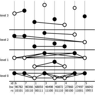
Figure 1: Example for the HSkip+ topology with eight nodes.

Figure 1 shows an example network with 8 nodes and 4 levels. The image visualizes the edges caused by the different levels in the HSkip+ topology.

2.2 HSkip+ Algorithm

To reach the presented topology, we now introduce a self-stabilizing algorithm whose correctness we will prove afterwards. All following operations are executed at node $v$. The algorithm works in the asynchronous message passing model presented in Section 1. We just use two types of guards: $true$ and $received(m)$. $true$ means that the action is continuously enabled, which implies that it is executed infinitely often. In addition to the definitions in Sec. 2.1 we take use of local variants (e. g. $\mathrm{localFarthestPred}(v,i)$) which represent the cached information at node $v$.

$true\rightarrow$ CheckNeighborhood() IntroduceNode() IntroduceClosestNeighbors() LinearizeNeighbors()

Figure 2: Action called periodically by node $v$.

The CheckNeighborhood() function checks if all nodes which are in the neighborhood of the node $v$ are needed for the topology (cf. Fig. 3). If a node $w$ is no longer needed in any level, it is removed from the neighborhood of $v$ and forwarded to another node $x$, concretely the node in the neighborhood with the longest common prefix, because it is the most promising node which could include the node in its own neighborhood at any level.

function CheckNeighborhood     for all $w\in v.nh$ do         if CheckNode($w$) = $false$ then            $v.nh=v.nh\backslash\{w\}$            send $m=(\mathrm{\emph{build}},w)$                      to node $\mathrm{argmax}_{x\in v.nh}{\mathrm{commonPrefix}(w,x)}$         end if     end for end function

Figure 3: CheckNeighborhood() inspects the nodes in $v.nh$.

The test if a node $w$ is really needed for node $v$ is done by the CheckNode() function (cf. Fig. 4). For the node $w$ in each level $i$ it is checked if the node $w$ is in the range (cf. Def. 6) of node $v$. If this is the case for at least one level, the node $w$ is needed in the neighborhood of $v$.

function CheckNode(node $w$)     $needed\leftarrow false$     for $i=0\text{ to }\mathrm{level}(v)$ do         if $\mathrm{prefix}(v,i)=\mathrm{prefix}(w,i)$                $\wedge(\mathrm{localFarthestPred}(v,i)=\bot$                     $\vee w.bw\leq\mathrm{localFarthestPred}(v,i).bw)$                $\wedge(\mathrm{localFarthestSucc}(v,i)=\bot$                     $\vee w.bw\geq\mathrm{localFarthestSucc}(v,i).bw)$            then            $needed\leftarrow true$         end if     end for     return $needed$ end function

Figure 4: CheckNode() tests if a node $w$ is needed in $v.nh$.

function IntroduceNode     for all $w\in v.nh$ do         send $m=(\mathrm{\emph{build}},v)$ to node $w$     end for end function

Figure 5: IntroduceNode() introduces the node $v$ to all neighbors.

function IntroduceClosestNeighbors     for $i=0\text{ to }\mathrm{level}(v)$ do         if $\mathrm{localClosestPred}(v,i)\neq\bot$ then            for all $w\in\mathrm{localNeighbors}(v,i)$ do                send $m=(\mathrm{\emph{build}},\mathrm{localClosestPred}(v,i))$                           to node $w$            end for         end if         if $\mathrm{localClosestSucc}(v,i)\neq\bot$ then            for all $w\in\mathrm{localNeighbors}(v,i)$ do                send $m=(\mathrm{\emph{build}},\mathrm{localClosestSucc}(v,i))$                           to node $w$            end for         end if     end for end function

Figure 6: IntroduceClosestNeighbors() introduces the closest neighbors.

function LinearizeNeighbors     for $i=0\text{ to }\mathrm{level}(v)$ do         for $j=0\text{ to }\left|\mathrm{localPredecessors}(v,i)\right|-1$ do            send $m=(\mathrm{\emph{build}},\mathrm{localPredecessors}(v,i)[j+1])$                      to $\mathrm{localPredecessors}(v,i)[j]$         end for         for $j=0\text{ to }\left|\mathrm{localSuccessors}(v,i)\right|-1$ do            send $m=(\mathrm{\emph{build}},\mathrm{localSuccessors}(v,i)[j+1])$                      to $\mathrm{localSuccessors}(v,i)[j]$         end for     end for end function

Figure 7: LinearizeNeighbors() introduces the neighbors to each other.

The other three periodic actions introduce new neighbors to each other to reach the desired topology. In the first function IntroduceNode(), node $v$ introduces itself to all of its neighbors to create backward edges (cf. Fig. 5). In the second function IntroduceClosestNeighbors(), node $v$ introduces the two direct neighbors, the closest predecessor and the closest successor, in each level to all other neighbors in this level (cf. Fig. 6). The last function LinearizeNeighbors() linearizes the neighborhood (cf. Fig. 7), i.e., each neighbor is introduced to the subsequent neighbor.

In addition to the periodic actions we have different reactive actions triggered by the $received(m)$ guard. Depending on the message type of the message $m$ received by a node $v$, the Build, Remove or Lookup operation is called (cf. Fig. 8).

$received(m)$ $\rightarrow$ if $m=(\mathrm{\emph{build}},x)$ then     $Build(x)$ else if $m=(\mathrm{\emph{remove}},x)$ then     $Remove(x)$ else if $m=(\mathrm{\emph{lookup}},x)$ then     $Lookup(x)$ end if

Figure 8: The incoming messages at node $v$ are handled.

The Build() function of a node $v$ must handle two cases (cf. Fig. 9): The node $x$ which is given as argument is already in the neighborhood or not. If it is already included, its information (especially its current bandwidth) is updated. Then the CheckNeighborhood() operation is called to check if the modified node $x$ and all other nodes are still needed for the node. In the case that the node $x$ is not yet in the neighborhood, it is checked by the CheckNode() function (cf. Fig. 4) if the node should be integrated in the neighborhood. If the node is needed in one level, it will be included in the neighborhood and the whole neighborhood will be checked if there is an unnecessary node now. If the new node is not needed by the node, it will be forwarded to the next node $w$ with the longest common prefix.

function Build(node $x$)     if $x\in v.nh$ then         update neighbor information         CheckNeighborhood()     else         $v.nh=v.nh\cup\{x\}$         if CheckNode($x$) = $true$ then            CheckNeighborhood()         else            $v.nh=v.nh\backslash\{x\}$            send $m=(\mathrm{\emph{build}},x)$                      to node $\operatorname{argmax}_{w\in v.nh}{\mathrm{commonPrefix}(x,w)}$         end if     end if end function

Figure 9: Build handles an incoming build message.

With these self-stabilizing rules the desired topology can be reached and maintained in a finite number of steps.

2.3 Correctness

Next we show the convergence and the closure of the algorithm, which implies that it is a self-stabilizing algorithm for the HSkip+ topology. Most of the proofs are skipped due to space constraints, but we dissected the self-stabilization process into sufficiently small pieces so that it is not too difficult to verify them with the help of the protocols.

2.3.1 Convergence

Here, we prove the following theorem:

Theorem 9 (Convergence).

If $G(t)=(V,E)$ is weakly connected at time $t$, then $G_{e}(t^{\prime})=G^{HSkip+}$ for some time $t^{\prime}>t$ and all node information is correct.

Proof.

To prove this theorem we will show different lemmas which lead to the convergence. But first, we give an overview of the whole proof: Starting with any weakly connected graph we first show that the network stays connected over time (cf. Lem. 10). Furthermore, we show that all wrong information about nodes in the network will be removed over time (cf. Lem. 11). Having reached this state, we will show the creation of the correct linked list at the bottom level (cf. Lem. 12) and the maintenance of it (cf. Lem. 13). The next step is the proof of the creation of the HSkip+ topology at the bottom level (cf. Lem. 14) and its maintenance (cf. Lem. 15). By showing the inductive creation of the HSkip+ topology at all levels (cf. Lem. 16) we can finish the convergence proof.

Note that edges are only deleted if there already exist other edges concerning the desired topology. Otherwise, edges are only added or delegated in a sense that a node $u$ holding an identifier of $v$ may forward that identifier to one of its neighbors $w$, which also preserves connectivity. Hence, we get:

Lemma 10 (Weakly Connected).

If $G(t)=(V,E)$ is weakly connected at time $t$, then $G(t^{\prime})$ is weakly connected at any time $t^{\prime}>t$.

Proof.

To show the connectivity, we have to prove that for all edges $(x,y)\in E(t)$ there is the same edge in the next time step, $(x,y)\in E(t+1)$, or there is a path from $x$ to $y$ which uses other edges. If the edge is still available in the next time step, $G(t+1)$ obviously stays weakly connected, so we only have to consider the case that $(x,y)\notin E(t+1)$. Here we distinguish between two different cases: Either the removed edge was an explicit edge or it was an implicit edge at time $t$.

So let us first consider the case where $(x,y)$ is an explicit edge in the graph and therefore $y$ is in the neighborhood of $x$. In our algorithm there is only one operation which removes nodes from the neighborhood: The CheckNeighborhood() function removes nodes which are not needed for the correct neighborhood. But in this case, a message with the removed node $y$ is sent by the current node $x$ to another node $v$ in its neighborhood (the one with the longest common prefix). Therefore, we have a new implicit edge $(v,y)$ and together with the existing explicit edge $(x,v)$ as $v$ is in the neighborhood of $x$, there exists a path from $x$ to $y$ over $v$.

We now look at the case where $(x,y)$ is an implicit edge at time $t$ which means that we have the reference to node $y$ in an incoming Build message at node $x$. The message is handled by the Build() operation and two cases can occur. On the one hand, the node $y$ can be useful in the neighborhood of $x$, then $y$ is integrated in the neighborhood and at time $t+1$, $y\in x.nh$. So we have an explicit edge instead of the implicit one. On the other hand, the node $y$ can be useless for the node $x$. Then $y$ is delegated to another node $v$ in its neighborhood (the one with the longest common prefix) and $x$ stays connected with $y$ over the node $v$ and the explicit edge $(x,v)$ ($v$ is in the neighborhood of $x$) as well as the new implicit edge $(v,y)$. ∎

Due to our FIFO delivery and fair message receipt assumption, all messages initially in the system will eventually be processed. Moreover, the distance (w.r.t. the sorted ordering of the nodes) of wrong information in the network can be shown to monotonically decrease. Once it is equal to one, the periodic self-introduction (cf. Figure 5) ensures that the node information is corrected, which implies the following lemma.

Lemma 11 (Wrong Information).

If $G(t)=(V,E)$ is weakly connected at time $t$, then there is a time point $t^{\prime}$ at which all node information in $G(t^{\prime\prime})$ is correct for any $t^{\prime\prime}>t^{\prime}$.

Proof.

We assume, that there is a wrong information in the network. This wrong information can be contained in a message or in an internal variable of a node. A message is only delegated a finite number of steps because it decreases the distance to its target in each step by choosing as next hop a node with a longer common prefix. Eventually, the information is integrated in the internal variables of a node, so we only have to consider this case. Therefore at a time $\hat{t}$, there is no wrong information in any message, but there can be wrong information in the internal variables of a node.

Assume that a node $x$ has wrong information about node $y$ at time $\hat{t}$. If node $x$ is connected to node $y$ by an explicit edge, eventually also node $y$ is connected to node $x$ because of the periodic call of IntroduceNode(). Periodically, $y$ sends a build message to $x$ in the IntroduceNode() function. This message is handled by the Build() operation in the first case ($y\in x.nh$). The information about $y$ in the internal variables of $x$ is updated and all wrong information is removed.

Furthermore, no new wrong information is produced in the network without any operations from outside, as only correct information is sent. Therefore at a time $t^{\prime}>t$ we have only correct information in the whole network. ∎

From now on, let us only consider time steps in which all node information is correct. Next to the edge set of the desired topology $E^{HSkip+}$ we define the edge set $E^{HSkip+_{i}}$ which contains all edges belonging to the topology at level $i$ and the edge set $E^{list_{i}}$ which contains all edges needed for a linked list at level $i$. Then it follows from arguments in [10] for the edge set $E^{list_{0}}$ at level 0:

Lemma 12 (List Creation).

If $G(t)=(V,E)$ is weakly connected, then $E_{e}(t^{\prime})\supseteq E^{list_{0}}$ at some time $t^{\prime}>t$.

Proof.

As the graph is weakly connected at time $t$, there exists an undirected path from $v$ to $w$ for all pairs $(v,w)\in V^{2}$. Now we look at two nodes $v$ and $w$ which should be direct neighbors: If $v$ and $w$ are already direct neighbors regarding their bandwidth values, then we only need one periodic message of the IntroduceNode() operation and we have the linked list completed at this point.

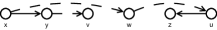
Figure 10: Path which connects $v$ with $w$ over intermediate nodes $y$, $x$, $u$, $z$.

Let us now assume without loss of generality, that the path from $v$ to $w$ is through other nodes (cf. Fig. 10). We will show that the length of the path from $v$ to $w$ does not increase and finally becomes shorter that in the end $v$ and $w$ are directly connected. At first, we will show that the length of the path does not increase: For each edge $(x,y)$ in the path it yields, that the edge is only replaced by two edges which are in the range of $(x,y)$. We distinguish two cases:

(a)

(b)

Figure 11: Edge $(x,y)$ is only replaced by two edges that are within the range of $(x,y)$.

1. $(x,y)$ is an implicit edge (cf. Fig. 11a):
   If the edge $(x,y)$ is not needed by $x$, there has to be a closer node $z$ in the neighborhood of $x$. As consequence, $y$ can be delegated to $z$ and the edge $(x,y)$ is replaced by the two edges $(x,z)$ and $(z,y)$ which fulfills the condition to stay in the range.

2. $(x,y)$ is an explicit edge (cf. Fig. 11b):
   The edge $(x,y)$ is only replaced if $x$ has a closer neighbor $z$ in its neighborhood. But than $y$ can be delegated to $z$ and the edge $(x,y)$ is replaced by the two edges $(x,z)$ and $(z,y)$ which fulfills the condition to stay in the range.

If $x$ has no further outgoing edge $(x,z)$, the edge $(x,y)$ is kept or integrated as explicit one since $x$ does not know about closer neighbors.

We now show that border nodes in the path (the leftmost and rightmost nodes) will eventually be eliminated. Therefore, we assume that the path from $v$ to $w$ contains a border node $x$. Without loss of generality, we assume that $x$ has the maximum bandwidth in the path, $x.bw>v.bw>w.bw$. There are various cases, how $x$ is connected with two edges to the path: Explicit or implicit, the edges may point to $x$ or away from $x$. The undirected path from $v$ to $w$ contains somewhere the successive sequence of the nodes $y$, $x$ and $z$ (w.l.o.g. $x.bw>y.bw>z.bw$). We want to exclude node $x$, so that the path only uses the nodes $y$ and $z$. We will now consider theses cases one by one:

(a)

(b)

(c)

(d)

Figure 12: The border node $x$ can be excluded from the path.

1. $x$ has explicit edges to $y$ and to $z$ (cf. Fig. 12a):
   With the LinearizeNeighbors() operation of node $x$, a new implicit edge $(y,z)$ is added since $y$ and $z$ are successive neighbors of $x$. We have a direct connection between $y$ and $z$ and $x$ can be excluded.

2. $x$ has an explicit edge to $y$ and an implicit one to $z$ (cf. Fig. 12b):
   Node $x$ integrates $z$ in its neighborhood, as it needs at least two successors. The edge $(x,z)$ is converted to an explicit edge and we have case a.

3. $x$ has an implicit edge to $y$ and an explicit edge to $z$ (cf. Fig. 12c):
   As in the previous case, Node $x$ integrates $y$ in its neighborhood since it needs at least two successors. The edge $(x,y)$ is also converted to an explicit one and we have case a.

4. $x$ has implicit edges to $y$ and to $z$ (cf. Fig. 12d):
   Depending on the order of processing, $y$ or $z$ is integrated in the neighborhood of $x$ since it has no successor. As consequence this case is reduced to case b or c.

Additionally, we have to consider the cases in which there is another node $u$ to which node $x$ has an explicit edge to:

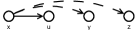
(a)

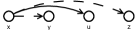
(b)

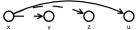
(c)

Figure 13: The border node $x$ can be excluded with the use of node $u$.

1. $x.bw>u.bw>y.bw>z.bw$ (cf. Fig. 13a):
   The results depends on the execution order: If the edge $(x,y)$ is considered first, $y$ is integrated in the neighborhood of $x$. In the next step with the LinearizeNeighborhood() operation, a new implicit edge $(u,y)$ is added since $u$ and $y$ are successive neighbors of $x$. We can treat $u$ as new $y$ and the case 1b holds.
   If $(x,z)$ is considered first, $z$ is integrated in the neighborhood, the implicit edge $(u,z)$ is added with the LinearizeNeighborhood() operation and with $u$ as new $z$, the case 1b also holds.

2. $x.bw>y.bw>u.bw>z.bw$ (cf. Fig. 13b):
   The same argumentation as in case 2a reduces to case 1b or 1c.

3. $x.bw>y.bw>z.bw>u.bw$ (cf. Fig. 13c):
   The same argumentation as in case 2a reduces to case 1b or 1c.

For the cases in which the edges point to $x$, a similar argumentation is possible to exclude the border node $x$. The exclusion of border nodes is executed for all border nodes on the undirected path from $v$ to $w$ until $v$ and $w$ are directly connected by an edge $(v,w)$ or $(w,v)$. Eventually, for each pair of direct neighbors $v$ and $w$ it yields that there is an edge $(v,w)\in E$ or $(w,v)\in E$. As the direct neighbors are always needed in our topology, the edges will be converted to explicit edges, if they are still implicit ones. By using one IntroduceNode() operation, the backward edges will be created for each pair and also integrated as explicit edges. Since now the double-linked list is completed at the base level, $G_{e}(t^{\prime})\supseteq G_{e}^{list_{0}}$ at time $t^{\prime}>t$. ∎

Moreover, it follows from the algorithm that the set of linked lists at level $i$, $E^{list_{i}}$, is maintained over time.

Lemma 13 (List Maintenance).

If $E_{e}(t)\supseteq E^{list_{i}}$ at time $t$, then $E_{e}(t^{\prime})\supseteq E^{list_{i}}$ at any time $t^{\prime}>t$.

Proof.

We start with a correct list $G_{e}^{list_{i}}$ at time $t$. As there are no external dynamics, no nodes enter or leave the system. To destroy the correct list, a node has to be removed from the neighborhood of any other node. The only removal happens in the CheckNeighborhood() operation after the check if the node is needed. But this check always returns true for the closest neighbors of a node because they are always needed. They are always in the range at level $i$ and CheckNode() returns $true$. Therefore no edges are removed and it follows that $G_{e}(t^{\prime})\supseteq G_{e}(t)\supseteq G_{e}^{list_{i}}$. ∎

Starting with a linked list at a level $i$ we can show the creation of the HSkip+ links at the same level, $E^{HSkip+_{i}}$:

Lemma 14 (HSkip+ Creation).

If $E_{e}(t)\supseteq E^{list_{i}}$ at time $t$, then eventually $E_{e}(t^{\prime})\supseteq E^{HSkip+_{i}}$ at time $t^{\prime}>t$.

Proof.

(a)

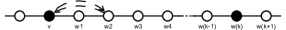
(b)

(c)

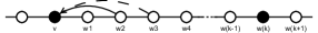
(d)

(e)

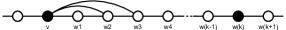
(f)

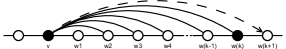
(g)

Figure 14: The correct creation of the skip+ edges for node $v$ at level $i$.

We start with a correct linked list $G_{e}^{list_{i}}$ which is created and obtained (cf. Lem. 12 and 13). We look at an arbitrary node $v$. It is connected to its direct predecessor $u_{1}$ and successor $w_{1}$, formally $\mathrm{localClosestPred}(v,i)=\mathrm{closestPred}(v,i)$ and $\mathrm{localClosestSucc}(v,i)=\mathrm{closestSucc}(v,i)$ (cf. Fig. 14a). The same holds for all other nodes, they are all connected to their direct predecessors and successors.

First we only look at the successors of node $v$. With the IntroduceClosestNeighbors() operation, node $w_{1}$ introduces the nodes $v$ and $w_{2}$ to each other and the implicit edges $(v,w_{2})$ and $(w_{2},v)$ are created (cf. Fig. 14b). As both edges are needed in the neighborhood of the nodes $v$ and $w_{2}$, they are both converted to explicit edges (cf. Fig. 14c).

Now node $w_{2}$ introduces $w_{3}$ to $v$ (cf. Fig. 14d). As the node $w_{3}$ is needed in the neighborhood of $v$ it is also converted to the explicit edge $(v,w_{3})$ and with the IntroduceNode() operation the implicit edge $(w_{3},v)$ is created (cf. Fig. 14e). Also this edge is converted to an explicit edge (cf. Fig. 14f).

The same procedure is continued for the nodes $w_{4},\ldots,w_{k}$ which are all needed neighbors for node $v$. Then the last neighbor $w_{k}$ introduces $w_{k+1}$ to node $v$ (cf. Fig. 14g). As it is not needed, it is not integrated in the neighborhood. This implicit edge is also created in the future by the IntroduceClosestNeighbors() operation of node $w_{k}$, but never converted to an explicit edge at level $i$. The successors are created correctly and the same observation can be made for the predecessors. Therefore, we eventually have all needed edges for the topology and $G_{e}(t)\supseteq G_{e}^{HSkip+_{i}}$. ∎

Additionally, it follows from our rules that the HSkip+ topology at a level $i$ is maintained over time.

Lemma 15 (HSkip+ Maintenance).

If $E_{e}(t)\supseteq E^{HSkip+_{i}}$ at time $t$, then $E_{e}(t^{\prime})\supseteq E^{HSkip+_{i}}$ at any time $t^{\prime}>t$.

Proof.

The proof is equivalent to the list maintenance (cf. Lem. 13): Explicit edges are only removed during the CheckNeighborhood() operation. As all neighbors are needed, no edge is removed and we get $G_{e}(t^{\prime})\supseteq G_{e}(t)\supseteq G_{e}^{HSkip+_{i}}$. ∎

Using the simple observation that $E^{list_{i+1}}\subseteq E^{HSkip+_{i}}$, we can then conclude:

Lemma 16 (HSkip+ Induction).

If $E_{e}(t)\supseteq E^{HSkip+_{i}}$ at time $t$, then $E_{e}(t^{\prime})\supseteq E^{HSkip+_{i+1}}$ at some time $t^{\prime}>t$.

Proof.

(a)

(b)

Figure 15: The inductive step from level $i$ to level $i+1$.

Starting with $G_{e}^{HSkip+_{i}}$, each node has an edge to the previous and one to next node with $0$ and $1$ as next bit of the bit string (cf. Fig. 15a). Each component of level $i$ is separated into two components of level $i+1$ according to the $i+1$-th bit. Furthermore, the components of the next level are already connected and they already form a double-linked list (cf. Fig. 15b). Now we can apply Lemma 14 and the correct HSkip+ topology is formed at level $i+1$ and maintained over the time (cf. Lem. 15). ∎

The previous lemmas immediately imply Theorem 9. ∎

2.3.2 Closure

After proving the convergence of our algorithm we need to show its closure. This means that the network stays in a legal state once it has reached one. Formally, we show (cf. Def. 2):

Theorem 17 (Closure).

If $G_{e}(t)=G^{HSkip+}$ at time $t$, then $G_{e}(t^{\prime})=G^{HSkip+}$ at any time $t^{\prime}>t$.

Proof.

Suppose that at time $t$ we have a network which forms the desired topology with its explicit edges, i.e., $E_{e}(t)=E^{HSkip+}$. If $E_{e}(t+1)\neq E_{e}(t)$, then at least one explicit edge is added or removed. Edges are only removed in the CheckNeighborhood() operation if they are not needed and edges are only added in the Build() operation if they are needed for the neighborhood. However, $G_{e}(t)$ already forms the correct neighborhood at time $t$ at all levels (cf. Def. 8). As there are no external changes and faults, the neighborhood is still correct at time $t+1$. Therefore, no edge is removed or added, so $G_{e}(t+1)=G_{e}(t)=G^{HSkip+}$. ∎

The convergence and closure together show the correctness of the self-stabilizing algorithm. In other words we have designed an algorithm which creates the HSkip+ topology and ensures that it stays correct.

2.4 External Dynamics

As external dynamics of a network we consider all events which can have an influence on the network. Two typical events for a peer-to-peer system are arrivals and departures of nodes. The network has to adapt the topology in this case. In our HSkip+ network we will also consider changes in the bandwidths of the nodes because also this will have an influence on the network topology. To handle these events we need a Join, Leave, and Change operation.

2.4.1 Join

The Join operation in our network is very simple. If a node $v$ wants to join the network, it just has to introduce itself to some node $w$. The rest will be handled by the self-stabilization. Hence, it suffices to execute the code in Fig. 16.

function Join     send $m=(\mathrm{\emph{build}},v)$ to a known node $w$ end function

Figure 16: The Join operation of node $v$ sends a build message to $w$.

2.4.2 Leave

We distinguish between two cases: A scheduled Leave and a Leave caused by a failure. In the first case (cf. Fig. 17) the node $v$ which wants to leave the network simply sends a remove message to all of its neighbors. The receivers of these messages remove the node $v$ from their neighborhood (cf. Fig. 18). The leaving node also deletes its entire neighborhood.

function Leave     for all $w\in v.nh$ do         send $m=(\mathrm{\emph{remove}},v)$ to node $w$     end for     $v.nh=\emptyset$ end function

Figure 17: The Leave() operation of node $v$ sends remove messages.

The Remove() operation removes a given node from the neighborhood if it is present (cf. Fig. 18). It is executed as reaction to a remove message. A neighborhood check is not needed, as there cannot be too much information after removing some information.

function Remove(node $x$)     if $x\in u.nh$ then         $u.nh=u.nh\backslash\{x\}$     end if end function

Figure 18: The Remove() operation removes the node $x$ from $v.nh$.

Additionally, we can have a Leave in the network caused by a node failure. In this case, we assume the existence of a failure detector at the nodes which checks periodically the existence of the neighbor nodes. Therefore, the outcome of a failed node is the same as for a scheduled Leave: all neighboring nodes invalidate their links to the failed node.

2.4.3 Change

The Change operation updates the bandwidth value of a node $v$ and therefore the order in our topology has to be updated. The operation itself only needs to update its internal variable of the bandwidth (cf. Fig. 19).

function Change(new bandwidth $bw$)     $v.bw=bw$ end function

Figure 19: The Change() operation updates the bandwidth value of $v$.

The correct recovery of the topology after no more external dynamics are happening follows directly from the convergence.

Theorem 18 (Recovery from External Dynamics).

If $G_{e}(t)=G^{HSkip+}$ at time $t$ and a node $v$ joins or a node $u$ leaves or a node $u$ changes its bandwidth, then eventually $G_{e}(t^{\prime})=G^{HSkip+}$ at time $t^{\prime}>t$.

Proof.

If the node $v$ joins the network by sending a build message to some node $w$, the graph has a new node $v$ and a new implicit edge $(w,v)$. Therefore $G(t+1)=\left(V(t+1)=V(t)\cup\{v\},E(t+1)=E(t)\cup\{(w,v)\}\right)$. $G(t+1)$ is obviously weakly connected. As there are no further external dynamics, we can apply the theorem about the convergence of our self-stabilizing algorithm (cf. The. 9). After a finite number of steps, we eventually reach the correct topology, formally $G_{e}(t^{\prime})=G^{HSkip+}$ at a time $t^{\prime}>t$. ∎

It is easy to see that the worst case number of structural changes in a level does not exceed $O(\log^{2}n)$ w.h.p., but with more refined arguments one can also show the following result:

Theorem 19 (Structural Changes after External Dynamics).

If $G_{e}(t)=G^{HSkip+}$ at time $t$ and a node $v$ joins or a node $u$ leaves or a node $u$ changes its bandwidth, then $G_{e}(t^{\prime})=G^{HSkip+}$ after $O(\log^{2}n)$ structural changes, w.h.p.

Proof.

To analyze the structural changes which are needed after node $v$ joins the network, we will look at the obsolete edges which have to be removed and at the new edges which need to be created during the self-stabilization.

As the degree of the network is limited by $O(\log n)$, each node $w$ has only $O(\log n)$ neighbors in $w.nh$. So each node can only remove at most $O(\log n)$ edges. Furthermore only $O(\log n)$ nodes can be affected from any changes as the new node $v$ can be in at most $O(\log n)$ neighborhoods and cause changes. Therefore at most $O(\log^{2}n)$ edges can be removed.

In addition, the new node $v$ has $O(\log n)$ other nodes in its neighborhood. As already stated in the removing part, only $O(\log n)$ other nodes are affected by the Join, each one can create at most $O(\log n)$ new edges. Therefore $O(\log n)+O(\log^{2}n)$ new edges can be created.

Altogether we have at most $O(\log^{2}n)$ structural changes in the network after a Join. ∎

With some effort, one can also show that this is an upper bound for the number of additional messages (i.e., messages beyond those periodically created by the $true$ guard).

Theorem 20 (Workload of External Dynamics).

If $G_{e}(t)=G^{HSkip+}$ at time $t$ and a node $v$ joins or a node $u$ leaves or a node $u$ changes its bandwidth, then $G_{e}(t^{\prime})=G^{HSkip+}$ after $O(\log^{2}n)$ additional messages, w.h.p.

Proof.

Firstly, the build message for the Join from node $v$ to node $w$ has to be forwarded to a node $x$ which can include the new node $v$ in its neighborhood. This needs at most $O(\log n)$ additional messages because the diameter of the network is at most $O(\log n)$ and the message will be forwarded closer to the target in each step as the bit string is adjusted at least one bit in each step.

At the position we need several further build messages to introduce and linearize the neighborhood. We have to create at most $O(\log^{2}n)$ structural changes (cf. Lem. 19). For each new edge, a message is created and integrated as an explicit edge in the next step. Therefore with $O(\log^{2}n)$ messages we can create all new edges. Altogether we have a workload of at most $O(\log^{2}n)$ additional messages to complete the Join operation. ∎

2.5 Routing

The routing of a message to a target node $x$ is handled by the message $m=(\text{\emph{lookup}},x)$. The Lookup() operation handles the forwarding of lookup messages (cf. Alg. 20). If the lookup target is equal to the current node, the lookup has finished. This is checked with the help of the identifiers of the nodes. If this is not the case, the lookup is forwarded to the next better node.

function Lookup(node $x$)     if $v.id=x.id$ then         done     else         $length$                $\leftarrow\min{(\mathrm{level}(v),\mathrm{commonPrefix}(v,x))}$         if $\mathrm{localFarthestPred}$                     $(v,length,x.rs[length])\neq nil$ then            $w\leftarrow\mathrm{localFarthestPred}$                          $(v,length,x.rs[length])$         else            $w\leftarrow\mathrm{localFarthestSucc}$                          $(v,length,x.rs[length])$         end if         send $m=(\mathrm{\emph{lookup}},x)$ to node $w$     end if end function

Figure 20: The Lookup() operation of $v$ handles the build messages.

The next hop is determined by the random bit strings of the involved nodes: In each step we want to have at least one bit more in common with the target node $x$. Formally, if at the current node $v$ the bit string has $i$ bits in common with the target ($\mathrm{commonPrefix}(v,x)=i$), at the next step at node $w$ we want at least $i+1$ bits in common ($\mathrm{commonPrefix}(w,x)\geq i+1$). In our topology such a node is always present in level $i$ of a node $v$ in both the successors and the predecessors (unless there is no such higher level) as every node is connected at every level $i$ to at least one predecessor and successor with $0$ and one with $1$ as next bit. First, the routing is done along predecessors so that the message is guaranteed to follow a sequence of nodes of monotonically increasing bandwidth. Once the node with the highest bandwidth defined by this rule has been reached, we use the successor nodes until the target node is reached. From the routing protocol it follows:

Theorem 21 (Correctness of Routing).

If $G_{e}=G^{HSkip+}$, then a message $m=(\mathrm{\emph{lookup}},w)$ sent by a node $u$ eventually reaches node $w$.

Proof.

We prove the correctness inductive such that at each step the random bit string $v.rs$ of the current node $v$ is more similar to the target bit string $x.rs$. As inductive hypothesis it holds that at step $i$ at node $v$: $\mathrm{prefix}(v,i)=\mathrm{prefix}(x,i)$. As induction base we look at step $i=0$ at the source node $s$, here at least the prefix of length $0$ should be equal to the target bit string, which obviously is the case. In the induction step we start from node $v$ with an equal prefix of length $i$ and the message has to reach a node $w$ with an equal prefix of length $i+1$. In the correct HSkip+ topology, each node has a predecessor and a successor with $0$ and $1$ as next bit. Only at the border nodes, the successor or predecessor could be absent, but at least one of the sides is complete. Therefore the length of the equal prefix is extended. As the target node $x$ exists in the network and is included in the HSkip+ topology it will eventually be reached by the message. ∎

We can also guarantee the following critical property, this is important to keep the congestion low.

Lemma 22 (Involved Nodes in Routing).

If $G_{e}=G^{HSkip+}$, the routing from some node $u$ to $w$ only uses nodes $v$ with $v.bw\geq\min{\{u.bw,w.bw\}}$.

The dilation is defined as the longest path which is needed to route a packet from an arbitrary source to an arbitrary target node. Since it just takes a single hop to climb up one level and there are at most $O(\log n)$ levels w.h.p., we get:

Theorem 23 (Dilation of Routing).

In HSkip+ the dilation is at most $O(\log n)$ w.h.p.

Proof.

In each routing step we use the edges of a higher level to forward the message to the next hop. As we have at most $O(\log n)$ levels, after $O(\log n)$ steps we have reached the highest level. At each step we have adjusted the bit string to reach the target bit string. At the highest level we have connections to all nodes with the same bit string and reach our target node directly. If this were not the case a further level would be included in the network because there would be a non trivial component (cf. Def. 4). Therefore, we need $O(\log n)$ steps to route a message from an arbitrary source to an arbitrary target and our dilation is $O(\log n)$. ∎

Finally, we analyze the congestion of our routing strategy. The congestion of a node $v$ is equal to the total volume of the messages passing it divided by its bandwidth. Let us consider the following routing problem: Each node $u$ selects a target bitstring $x$ independently and uniformly at random and sends a message of volume $\min\{u.bw,w.bw\}$ to the node $w$ with the longest prefix match with $x$. Of course, $u$ may not know that volume in advance. Our goal will just be to show that the expected congestion of this routing problem is $O(\log n)$. If this is the case, then one can show similar to [4] that the expected congestion of routing any routing problem in HSkip+ is by a factor of at most $O(\log n)$ worse than the congestion of routing that routing problem in any other topology of logarithmic degree, which matches the result in [4].

Theorem 24 (Congestion of Routing).

In the HSkip+ topology, we can route messages with the presented routing algorithm (cf. Alg. 20) and the defined routing problem with an expected congestion of $O(\log n)$.

To prove the congestion we divide the routing process of a message from an arbitrary source node $u$ to an arbitrary target node $w$ into two parts: On the one hand the routing from $u$ along predecessor edges to an intermediate node $v$ which has no better predecessors and on the other hand the routing back over successors from node $v$ to the target node $w$. We will start with the first part of the routing process, and initially we separately look at each level $i$ in the network at node $v$. Later, we will sum it up for all levels.

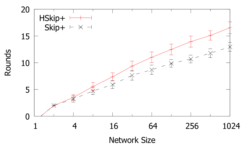
Figure 21: Stabilization Time.

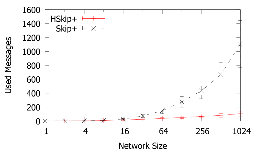
Figure 22: Overall Used Messages Total.

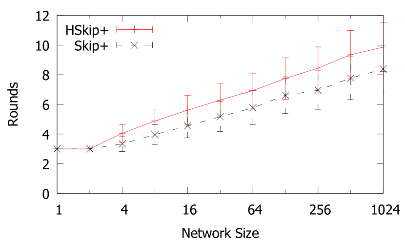
Figure 23: Stabilization Time after Join.

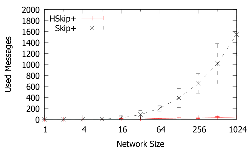
Figure 24: Used Messages after Join.

Lemma 25 (Congestion of node $v$ at level $i$).

In our routing problem (cf. The. 24), every node $v$ has an expected congestion of $O(1)$ at every level $i\geq 1$.

Proof.

We assume w.l.o.g. that the first $i$ bits of $v.rs$ are $1$. So messages with the target bitstring starting with $1\ldots 1$ as the first $i$ bits will be sent through the node $v$ as long as they start at a node $w$ that, at level 0, is between $v$ and the closest successor $w^{\prime}$ of $v$ whose first $i$ bits are also 1. We calculate the probability that there are $m$ nodes between $v$ and $w^{\prime}$. For each node in between we have the probability $(1-(\frac{1}{2})^{i})$ that one of its first $i$ bits differs from 1, and for $w^{\prime}$ we get a probability of $(\frac{1}{2})^{i}$ that its first $i$ bits are 1. Altogether, we get a probability that there are $m$ sources that may send their messages to $v$ of $(1-(\frac{1}{2})^{i})^{m}\cdot(\frac{1}{2})^{i}=\frac{(2^{i}-1)^{m}}{(2^{i})^{m+1}}$. Furthermore, we have to estimate the fraction of messages which will be sent through $v$. Each message is sent through $v$ if the first $i$ bits are $1$, which has a probability of $\frac{1}{2^{i}}$. Since we have $m$ possible sources (excluding $v$), a fraction of $(m+1)\cdot\frac{1}{2^{i}}$ messages will be sent through $v$. Lastly, we have to look at the volume sent by a single source. We know that a node $s$ can send at most a volume of $s.bw$. As we have only successors of $v$ as sources and for all successors $s$ it holds that $s.bw<v.bw$, we can upper bound the volume sent by each source by $v.bw$. Altogether, if we have $m$ nodes between $v$ and $w^{\prime}$, the total expected volume through $v$ at level $i$ is at most $(m+1)\cdot\frac{1}{2^{i}}\cdot v.bw$. Let the random variable $X_{v}^{i}$ be the total volume sent through $v$ at level $i$. Then

$$E\left[X_{v}^{i}\right]=\sum_{m=0}^{\infty}{\frac{(2^{i}-1)^{m}}{(2^{i})^{m+1}}\cdot(m+1)\cdot\frac{1}{2^{i}}\cdot v.bw}=O(v.bw)$$

∎

Summing up the congestion over all levels, we get:

Lemma 26 (Congestion of node $v$).

In our routing problem (cf. The. 24), an arbitrary node $v$ has an expected congestion of $O(\log{n})$.

Proof of Theorem 24.

With the previous lemmas (cf. Lem. 25 and Lem. 26) we have calculated the congestion caused by the first part of the routing process. For the second part, we can argue in a similar way by looking at the routing path backwards from the target node $x$ to the intermediate node $v$ and we also get an expected volume of $O(\log n)\cdot v.bw$ at node $v$. Both routing parts together yield an expected congestion of $O(\log n)$ at every node $v$. ∎

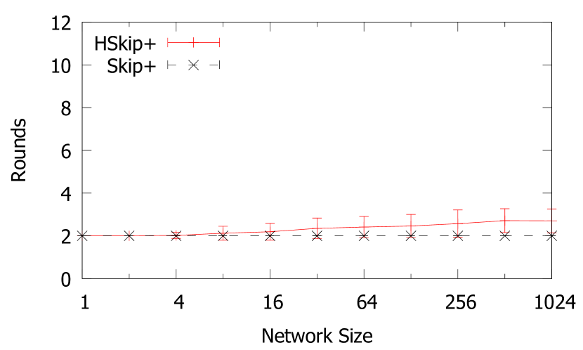
Figure 25: Stabilization Time after Leave.

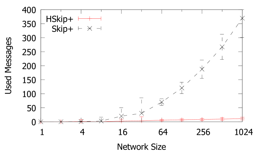
Figure 26: Used Messages after Leave.

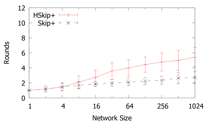
Figure 27: Stabilization Time after Change.

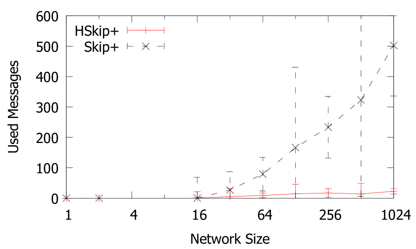
Figure 28: Used Messages after Change.

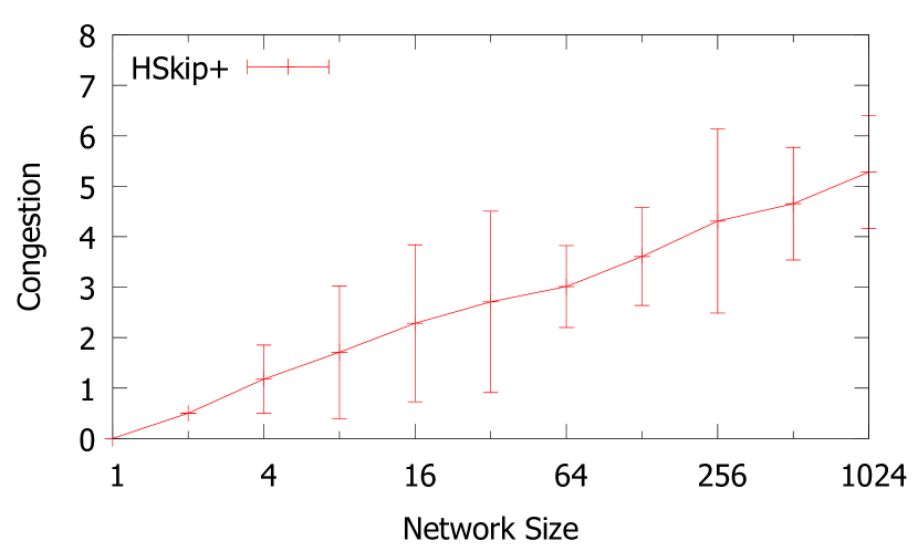
Figure 29: Routing Congestion of Flow Problem.

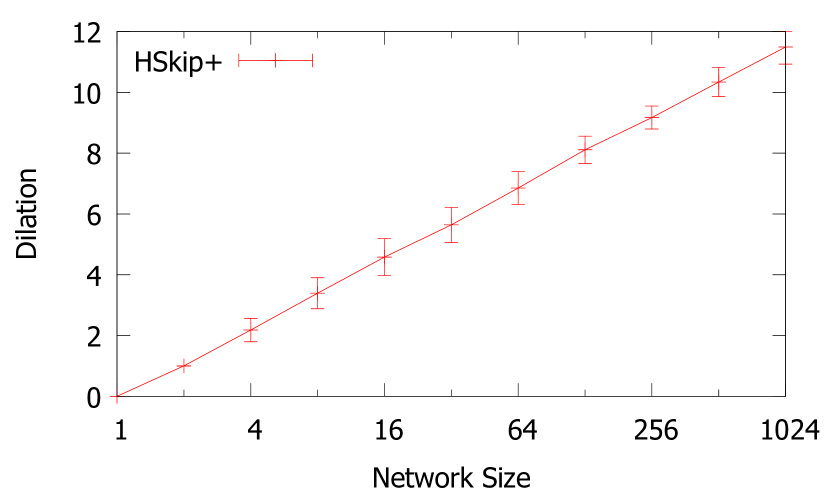
Figure 30: Routing Dilation of Flow Problem.

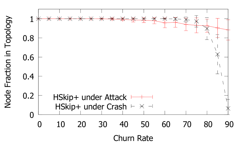
Figure 31: Stabilization after Crash and Attack.

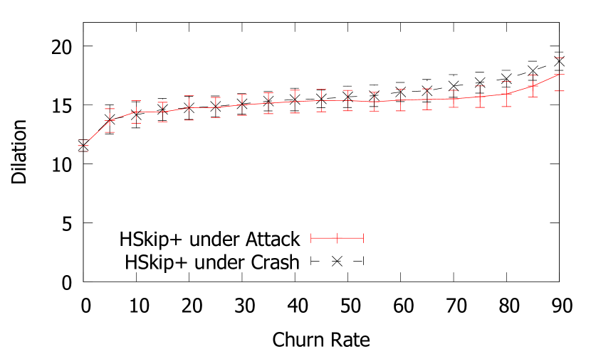
Figure 32: Routing Dilation during Crash and Attack.

3 Simulations

In this section we present simulation results for the HSkip+ network in comparison to the Skip+ graph. We simulated both protocols starting from randomly generated trees. The bandwidths were assigned randomly to the peers according to measurements of the connections in Germany [5]. All simulations are run 100 times with different seeds for network configurations with up to 1024 participating nodes. Since both networks are self-stabilizing, we focus on the stabilization costs in terms of rounds (in each round every node is allowed to process all received messages) until the desired topology is constructed from an initial weakly connected network and the number of messages which were used in this process. The simulator can be found in the ancillary files of this paper on arXiv.org.

3.1 Self-Stabilization

If we look at the self-stabilization time for Skip+ and HSkip+ (cf. Fig. 22), we see asymptotically similar results. Both networks need $O(\log n)$ rounds for the self-stabilization, whereas the Skip+ has slightly better results. In contrast, if we look at the used messages (cf. Fig. 22), we see a big difference between both networks. While Skip+ uses $O(\log^{4}n)$ messages for the self-stabilization process, the HSkip+ topology requires only $O(\log^{2}n)$ messages.

3.2 External Dynamics

As the next step, we look at the external dynamics in the network, namely joining and leaving nodes, as well as bandwidth changes. We start with the needed rounds after a new node joined the network (cf. Fig. 24). The result is similar to the self-stabilization we have seen before. Both networks are stabilized again after $O(\log n)$ rounds, where the Skip+ network is slightly faster. Also the overall used messages for this process reflect the already seen result (cf. Fig. 24). While the Skip+ network consumes $O(\log^{4}n)$ messages, the rules of HSkip+ need only $O(\log^{2}n)$ messages. The concrete number of messages are not directly comparable to the numbers in Fig. 22 as there are further messages in the system which cannot be excluded from counting.

Also the other two operations show similar results. The self-stabilization after a node left the network or changed its bandwidth can be finished in $O(\log n)$ rounds and nearly in constant time (cf. Fig. 26 and 28). This tendency yields also for the used messages. The work consumed by HSkip+ is clearly less than in the case of Skip+ (cf. Fig. 26 and 28).

3.3 Routing

For evaluating the routing performance of the topology we look at a flow problem: For each node pair $u,v\in V$ node $u$ sends an amount of data of $\frac{u.bw\cdot v.bw}{\sum_{w\in V}{w.bw}}$ to node $v$. The average normalized congestion (according to the nodes’ bandwidth) is logarithmic in the network size (cf. Fig. 30). The same yields for the dilation of the routing process (cf. Fig. 30). Both results agree with the theoretical findings as proved in Sec. 2.5.

3.4 Behavior under Churn

As last aspect we look at the network behavior under churn. In a practical usage scenario of a peer-to-peer system nodes can arbitrary join and leave the network. Usual churn behavior as it was studied in several papers (i.e. [17, 22]) has no influence on the topology as the stabilization times of our network are significantly smaller than the session and intersession times of peers in a network. Therefore, we focus on two exceptional scenarios: On the one hand we examined a crash and on the other hand an adversarial attack. In the first scenario x% randomly chosen nodes are leaving from a network with 1024 nodes at the same time and the same number of new nodes join the network (to have a comparable size of the network). In the second scenario the leaving nodes are no longer randomly chosen, but all from a neighboring area.

The number of leaving nodes has no remarkable influence on the stabilization time as we have seen it in Fig. 24, Fig. 26 and Fig. 28. Hence, we concentrate on the topology after stabilization and especially how many nodes are still connected correctly (cf. Fig. 32). Up to a churn rate of about 35% all nodes stay in the topology, under a random crash even up to a rate of 60%. Over this limit, the topology looses nodes which are no longer reachable. As for the second evaluation, we concentrate on the dilation. We have used the same flow problem as in Sec. 3.3 starting at the same round as the attack and crash. In a stable network with 1024 nodes, it is about 11 hops (cf. Fig. 30). During the attack or crash it is just a little increased to about 14 or 15 hops; only at a very high churn rate (when we also have lost many nodes) the dilation increases noticeable.

4 Conclusion

In this paper, we presented HSkip+, a self-stabilizing overlay network based on Skip+. We showed by simulations that the self-stabilization time is nearly identical in $O(\log n)$ while the improved version uses only $O(\log^{2}n)$ messages for the process compared to the originally used $O(\log^{4}n)$ messages. Also the dealing with external dynamics can be managed in the same time bounds and with the same work. Furthermore, we have extended the network to deal with heterogeneous bandwidths where we reach a logarithmic congestion and dilation in the routing process. Finally, the practical usage was shown by simulations under churn behavior.

References

- [1] J. Aspnes and G. Shah. Skip graphs. In Proceedings of the ACM-SIAM Symposium on Discrete Algorithms (SODA ’03), pages 384–393. Society for Industrial and Applied Mathematics, 2003.
- [2] B. Awerbuch and C. Scheideler. The hyperring: a low-congestion deterministic data structure for distributed environments. In Proceedings of the fifteenth annual ACM-SIAM symposium on Discrete algorithms, SODA ’04, pages 318–327, Philadelphia, PA, USA, 2004. Society for Industrial and Applied Mathematics.
- [3] A. Berns, S. Ghosh, and S. V. Pemmaraju. Building self-stabilizing overlay networks with the transitive closure framework. In Proceedings of the International Conference on Stabilization, Safety, and Security of Distributed Systems (SSS ’11), pages 62–76, 2011.
- [4] A. Bhargava, K. Kothapalli, C. Riley, C. Scheideler, and M. Thober. Pagoda: a dynamic overlay network for routing, data management, and multicasting. In Proceedings of the ACM Symposium on Parallelism in Algorithms and Architectures (SPAA ’04), pages 170–179, 2004.
- [5] Bundesnetzagentur für Elektrizität, Gas, Telekommunikation, Post und Eisenbahnen. Tätigkeitsbericht 2012/2013, 2013.
- [6] E. W. Dijkstra. Self-stabilizing systems in spite of distributed control. Communications of the ACM, 17(11):643–644, Nov. 1974.
- [7] S. Dolev and R. I. Kat. HyperTree for Self-Stabilizing Peer-to-Peer Systems. In Proceedings of the IEEE International Symposium on Network Computing and Applications (NCA ’04), pages 25–32, 2004.
- [8] S. Dolev and N. Tzachar. Spanders: Distributed spanning expanders. Sci. Comput. Program., 78(5):544–555, May 2013.
- [9] D. Gall, R. Jacob, A. Richa, C. Scheideler, S. Schmid, and H. Täubig. Time complexity of distributed topological self-stabilization: the case of graph linearization. In Proceedings of the Latin American Conference on Theoretical Informatics (LATIN ’10), pages 294–305, 2010.
- [10] R. Jacob, A. Richa, C. Scheideler, S. Schmid, and H. Täubig. A distributed polylogarithmic time algorithm for self-stabilizing skip graphs. In Proceedings of the ACM Symposium on Principles of Distributed Computing (PODC ’09), pages 131–140, 2009.
- [11] R. Jacob, S. Ritscher, C. Scheideler, and S. Schmid. Towards higher-dimensional topological self-stabilization: A distributed algorithm for Delaunay graphs. Theor. Comput. Sci., 457:137–148, Oct. 2012.
- [12] S. Kniesburges, A. Koutsopoulos, and C. Scheideler. Re-Chord: a self-stabilizing chord overlay network. In Proceedings of the ACM Symposium on Parallelism in Algorithms and Architectures (SPAA ’11), pages 235–244, 2011.
- [13] S. Kniesburges, A. Koutsopoulos, and C. Scheideler. CONE-DHT: A Distributed self-stabilizing algorithm for a heterogeneous storage system. In Proceedings of the International Symposium on Distributed Computing (DISC’13), 2013.
- [14] R. Meier and R. Wattenhofer. Peer-to-Peer Streaming in Heterogeneous Environments. Signal Processing: Image Communication, 27(5):457–469, March 2012.
- [15] W. Nejdl, M. Wolpers, W. Siberski, C. Schmitz, M. Schlosser, I. Brunkhorst, and A. Löser. Super-peer-based routing and clustering strategies for RDF-based peer-to-peer networks. In Proceedings of the ACM International Conference on World Wide Web (WWW ’03), pages 536–543, 2003.
- [16] R. M. Nor, M. Nesterenko, and C. Scheideler. Corona: a stabilizing deterministic message-passing skip list. In Proceedings of the International Conference on Stabilization, Safety, and Security of Distributed Systems (SSS ’11), pages 356–370, 2011.
- [17] K. Pussep, C. Leng, and S. Kaune. Modeling User Behavior in P2P Systems. In K. Wehrle, M. Günes, and J. Gross, editors, Modeling and Tools for Network Simulation, pages 447–461. Springer, 2010.
- [18] C. Scheideler and S. Schmid. A Distributed and Oblivious Heap. In Proceedings of the Internatilonal Collogquium on Automata, Languages and Programming (ICALP ’09), pages 571–582, 2009.
- [19] M. Schneider. Self-stabilization. ACM Computing Surveys, 25(1):45–67, Mar. 1993.
- [20] A. Shaker and D. S. Reeves. Self-Stabilizing Structured Ring Topology P2P Systems. In Proceedings of the IEEE International Conference on Peer-to-Peer Computing (P2P ’05), pages 39–46, 2005.
- [21] M. Srivatsa, B. Gedik, and L. Liu. Scaling Unstructured Peer-to-Peer Networks With Multi-Tier Capacity-Aware Overlay Topologies. In Proceedings of the IEEE Parallel and Distributed Systems, Tenth International Conference (ICPADS ’04), 2004.
- [22] M. Steiner, T. En-Najjary, and E. W. Biersack. Long term study of peer behavior in the KAD DHT. IEEE/ACM Trans. Netw., 17(5):1371–1384, 2009.