Random matrix study for a three-terminal chaotic device

Abstract

We perform a study based on a random-matrix theory simulation for a three-terminal device, consisting of chaotic cavities on each terminal. We analyze the voltage drop along one wire with two chaotic mesoscopic cavities, connected by a perfect conductor, or waveguide, with one open mode. This is done by means of a probe, which also consists of a chaotic cavity that measure the voltage in different configurations. Our results show significant differences with respect to the disordered case, previously considered in the literature.

I Introduction

In the last thirty years there have been much theoretical and experimental work concerning electronic transport through multiterminal devices (see Refs. Datta ; Goodnick there in). Nowadays, the interest to study the electronic transport properties on these devices has been renewed Picciotto ; Chang ; Geisel ; Haan ; Gao ; Aita , due to the fact that they are very useful in experimental measurements in several configurations ButtikerPRA ; ButtikerPRL ; ButtikerIBM .

The earlier experiments were done with normal metal conductors, whose random distribution of impurities in their microscopic structure, give rise to interference that is reflected in the relevant physical observables, like resistance or voltage measurements. Moreover, those quantities show sample to sample fluctuations GodoyEPL ; Godoy ; GMM1 . More recently, the interest on these systems has resurged due to recent advances in technology, that allow to access to clean devices, where the typical size is smaller than the elastic mean free path. Therefore, the electrons propagate ballistically and scattering is produced only by the device boundaries, which have important consequences in the electronic transport through the device Haan ; Song1 ; Song2 . For instance, when the geometry is such that the classical dynamics in the system is chaotic, the transport properties fluctuates too MelloLesHouches ; BeenakkerRMP ; Alhassid . What is very important is to know how are the fluctuations with respect to the disordered case.

In this work, by numerical simulation, we analyze the statistical distribution of the voltage drop along a chaotic wire, which consists of two chaotic mesoscopic cavities connected by a perfect conductor with one open mode. The probe is a chaotic cavity that measure the voltage in different configurations. The presence and absence of time reversal invariance are considered. We compare our results with the ones obtained in an equivalent three terminal device but with disordered, instead of chaotic, wires, previously studied in the literature, where the distribution of the voltage drop was determined in the presence of time reversal invariance only GodoyEPL ; Godoy . There, a remarkable difference in the distribution of the voltage drop between the ballistic regime and the strong disordered limit, has been found. The position of the probe has a stronger effect than in the disordered case.

First, we summarize the scattering formalism for the voltage drop in a three terminal device, proposed by Büttiker ButtikerPRL ; ButtikerIBM . Then, we construct the scattering matrix for our system, in terms of the scattering matrices of the individual cavities, as well as of the scattering matrix associated to the junction, for which we assume the simplest model introduced by Büttiker, that couple the probe symmetrically to the horizontal wire ButtikerPRA . For the statistical analysis, we make an ensemble of systems by assuming that the scattering matrix of each cavity is chosen from a Circular Ensemble, Orthogonal or Unitary, depending on the presence or absence of time reversal invariance. We present our conclusions at the end.

II Electronic transport in a three-terminal system

In the formulation of Landauer-Büttiker, the electronic transport is reduced to a scattering problem. In a single mode multiprobe devices, the current $I_{i}$ in a lead $i$ can be written into two components, one being the reflection to the same lead and the transmission from the others leads to the lead $i$. That is, $I_{i}$ is given in terms of the reflection and transmission coefficients, according to ButtikerIBM

$$I_{i}=\frac{e}{h}\left[(1-R_{ii})\mu_{i}-\sum_{j\neq i}T_{ij}\mu_{j}\right],$$ (1)

where $\mu_{j}$ is the chemical potential in lead $j$, $R_{ii}$ is the reflection coefficient to the lead $i$, and $T_{ij}$ represent the transmission from lead $j$ to lead $i$. These coefficients are given by the scattering matrix $S$ as $R_{ii}=|S_{ii}|^{2}$ and $T_{ij}=|S_{ij}|^{2}$.

The voltage along a horizontal wire, connected via perfect leads to two reservoirs of fixed chemical potentials, $\mu_{1}$ and $\mu_{2}$, can be measured in a three terminal device, where the third wire is in a voltage measurement configuration (see Fig. 1); that is, the chemical potential $\mu_{3}$ is such that the current through it is equal to zero, $I_{3}=0$. In such a case ButtikerIBM ,

$$\mu_{3}=\frac{1}{2}(\mu_{1}+\mu_{2})+\frac{1}{2}(\mu_{1}-\mu_{2})f,$$ (2)

where $f$ is given by

$$f=\frac{T_{31}-T_{32}}{T_{31}+T_{32}}.$$ (3)

Equation (2) shows that the chemical potential $\mu_{3}$ has an averaged part, that comes from the effect of the resorvoirs $\mu_{1}$ and $\mu_{2}$ only. The second part gives the deviation from the averaged part, and depends on the intrinsic nature of the conductors through the quantity $f$, that contains all the relevant information about the multiple scattering in the device. If the conductors are disordered or chaotic, $f$ fluctuates between -1 and 1, since $\mu_{3}$ can not reach the values $\mu_{1}$ nor $\mu_{2}$ due to the contact resistance ButtikerIBM . The disordered three terminal device was studied in Refs. GodoyEPL ; Godoy .

In what follows we will consider a three terminal device where the conductors are chaotic. Since $f$ depends on the scattering matrix $S$ of the whole system, we construct $S$ in terms of the scattering matrices of each conductor and the scattering matrix of the splitter, that we will assume to be known. For the splitter we assume a simple model, while the scattering matrices of the chaotic conductors are chosen from an ensemble of random matrices that satisfy certain symmetry requirements.

Figure 1: A scattering system consisting of three one-dimensional wires converging to a junction. The thin lines represent perfect conductors that connect the wave guides to the chemical reservoirs. The amplitude of the incoming (outgoing) wave in wire $i$ is denoted by $a_{i}$ ($b_{i}$), while $a^{\prime}_{i}$ ($b^{\prime}_{i}$) denotes the amplitude at the junction. Each wire is described by a $2\times 2$ scattering matrix $S_{j}$ and the junction by a $3\times 3$ matrix, $S_{0}$.

III The $S$ matrix for a three terminal device

Let us consider the three terminal system shown in Fig. 1. The system is described by the scattering matrix $S$ which relates the incoming plane waves amplitudes on each terminal, $a_{1}$, $a_{2}$, and $a_{3}$, to the outgoing ones, $b_{1}$, $b_{2}$, and $b_{3}$, by

$$\left(\begin{array}[]{c}b_{1}\\ b_{2}\\ b_{3}\end{array}\right)=S\left(\begin{array}[]{c}a_{1}\\ a_{2}\\ a_{3}\end{array}\right),$$ (4)

where we assume that $S$ contains all the information that from the system we can obtain. Of course, $S$ depends on the scattering process inside the system, due to scattering elements.

Let assume that the splitter is represented by the scattering matrix $S_{0}$, that couples the three terminals; therefore, the amplitudes at the junction are related as

$$\left(\begin{array}[]{c}b^{\prime}_{1}\\ b^{\prime}_{2}\\ b^{\prime}_{3}\end{array}\right)=S_{0}\left(\begin{array}[]{c}a^{\prime}_{1}\\ a^{\prime}_{2}\\ a^{\prime}_{3}\end{array}\right).$$ (5)

If the conductors on each terminal are represented by the scattering matrices $S_{j}$ ($j=1,2,3$), the amplitudes are related as follows:

$$\left(\begin{array}[]{c}b_{1}\\ a^{\prime}_{1}\end{array}\right)=S_{1}\left(\begin{array}[]{c}a_{1}\\ b^{\prime}_{1}\end{array}\right),\quad\left(\begin{array}[]{c}a^{\prime}_{2}\\ b_{2}\end{array}\right)=S_{2}\left(\begin{array}[]{c}b^{\prime}_{2}\\ a_{2}\end{array}\right),\quad\left(\begin{array}[]{c}a^{\prime}_{3}\\ b_{3}\end{array}\right)=S_{3}\left(\begin{array}[]{c}b^{\prime}_{3}\\ a_{3}\end{array}\right),$$ (6)

where each matrix $S_{j}$ is a $2\times 2$ matrix with the general structure

$$S_{j}=\left(\begin{array}[]{cc}r_{j}&t^{\prime}_{j}\\ t_{j}&r^{\prime}_{j}\\ \end{array}\right),$$ (7)

with $r_{j}$, $t_{j}$ are the reflection and transmission amplitudes when the incidence is from the left (or below for $j=3$) of the $j$th conductor, and $r^{\prime}_{j}$, $t^{\prime}_{j}$ when the incidence is from the other side. Flux conservation implies that $S_{j}$ is unitary,

$$S_{j}S_{j}^{\dagger}=I_{2},$$ (8)

where $I_{2}$ stands for the $2\times 2$ identity matrix. Equation (8) is the only requirement in absence of any symmetry, while in the presence of time reversal invariance, $S_{j}$ is a unitary and symmetric,

$$S_{j}=S_{j}^{T},$$ (9)

where $T$ stands for the transposed.

Through Eqs. (5), (7) and (6) we arrive to the scattering matrix $S$ that describes the full system, which is given by

$$S=S_{PP}+S_{PQ}S_{0}\frac{1}{1-S_{QQ}S_{0}}S_{QP},$$ (10)

where we have defined

$$S_{PP}=\left(\begin{array}[]{ccc}r_{1}&0&0\\ 0&r^{\prime}_{2}&0\\ 0&0&r^{\prime}_{3}\end{array}\right),\qquad S_{PQ}=\left(\begin{array}[]{ccc}t^{\prime}_{1}&0&0\\ 0&t_{2}&0\\ 0&0&t_{3}\end{array}\right),\qquad S_{QP}=\left(\begin{array}[]{ccc}t_{1}&0&0\\ 0&t^{\prime}_{2}&0\\ 0&0&t^{\prime}_{3}\end{array}\right),\qquad S_{QQ}=\left(\begin{array}[]{ccc}r^{\prime}_{1}&0&0\\ 0&r_{2}&0\\ 0&0&r_{3}\end{array}\right).$$ (11)

Equation (10) has a nice interpretation: the first term on the right hand side, $S_{PP}$, represents the reflected parts of the waves that reach the conductors, while the second term comes from the multiple scattering in the system. Here, $S_{QP}$ gives the transmission from outside to inside, $S_{PQ}$ gives the transmission from inside to outside of the system, and $S_{QQ}$ represents the internal reflections.

Notice that $S$ is also a unitary matrix once we ensure that $S_{0}$ is chosen as a unitary matrix too, and the symmetry conditions are fixed by the symmetry properties of the $S_{j}$’s. Although our result is general, in what follows we adopt a simple model for $S_{0}$ and we choose $S_{j}$ from an ensemble of scattering matrices that simulates chaotic cavities.

III.1 A simple model for the splitter

A simple model for the $S$-matrix of the splitter, real and symmtric, that couples the probe symmetrically, was proposed by Büttiker ButtikerPRA , namely

$$S_{0}=\left(\begin{array}[]{ccc}a&b&\sqrt{\varepsilon}\\ b&a&\sqrt{\varepsilon}\\ \sqrt{\varepsilon}&\sqrt{\varepsilon}&-(a+b)\end{array}\right),$$ (12)

where $\varepsilon$ is a real parameters with $0\leq\varepsilon\leq 1/2$, which gives the coupling strength, and

$$a=-\frac{1}{2}\left(1-\sqrt{1-2\varepsilon}\right),\quad b=+\frac{1}{2}\left(1+\sqrt{1-2\varepsilon}\right).$$ (13)

When the coupling vanishes ($\varepsilon\rightarrow 0$), $a\rightarrow 0$ and $b\rightarrow 1$ which means that the probe is decoupled and there is complete transmission between the terminals 1 and 2. On the contrary, when the probe is perfectly coupled ($\varepsilon=1/2$), $a=-1/2$ and $b=1/2$, nothing is reflected to the probe.

IV The voltage measurement

We assume that the conductors in our device are in fact chaotic cavities, such that the voltage measurement, and any other transport properties, shows sample to sample fluctuations, although macroscopically seems to be identical; this is due to the difficulty of control of the shape of the cavity microscopically. Of course, the fluctuations also arise with respect to external parameters like the chemical potentials and magnetic field. Therefore, we require to make a statistical study for the voltage measurement. We do this for two kind of ensembles for the $S_{j}$ matrices: in presence and absence of time reversal symmetry. In the Dyson’s scheme these correspond to the orthogonal and unitary cases, labeled by $\beta=1$ and $\beta=2$, respectively Dyson1962 .

IV.1 Presence of time reversal invariance

In the $\beta=1$ symmetry, an $S_{j}$ matrix can be parameterized in a “polar representation” as MelloLesHouches

$$S_{j}=\left(\begin{array}[]{cc}e^{i\phi_{j}}&0\\ 0&e^{i\psi_{j}}\end{array}\right)\left(\begin{array}[]{cc}-\sqrt{1-\tau_{j}}&\sqrt{\tau_{j}}\\ \sqrt{\tau_{j}}&\sqrt{1-\tau_{j}}\end{array}\right)\left(\begin{array}[]{cc}e^{i\phi_{j}}&0\\ 0&e^{i\psi_{j}}\end{array}\right),$$ (14)

where $\phi_{j}$ and $\psi_{j}$ are random numbers, uniformly distributed in the interval $[0,2\pi]$, and $\tau_{j}$ is randomly distributed in $[0,1]$. The probability distribution for $S_{j}$ is MelloLesHouches

$$dP_{1}(S_{j})=\frac{d\tau_{j}}{2\sqrt{\tau_{j}}}\frac{d\phi_{j}}{2\pi}\frac{d\psi_{j}}{2\pi},$$ (15)

which defines the Circular Orthogonal Ensemble, which can be generated numerically. Once this is done, we substitute the elements of the $S_{j}$ matrices in the expressions given in Eq. (11), and then in Eq. (10) from which we obtain the transmission coefficients $T_{31}$ and $T_{32}$, needed to determine $f$ through Eq. (3).

The numerical results for the distribution of $f$, for several values of the coupling strength $\varepsilon$, are shown in Fig. 2 for different measurement configurations. Panels (a), (b), and (c) of this figure are the most general cases of voltage measurements with respect to the position, where all conductors are chaotic. We can observe a clear dependence on the position of the probe. In panel (a), the probe is in the middle of the horizontal wire, and the distribution of $f$ is symmetric around zero, which means that $\mu_{3}$ fluctuates symmetrically around the average $(\mu_{1}+\mu_{2})/2$. However, when the position of the probe changes to one end of the horizontal wire, the distribution of $f$ is no more symmetric with respect to zero, as can be seen in panels (b) and (c) of Fig. 2; in fact, $\mu_{3}$ tends to be closer to the chemical potential of that terminal. We also note that the distribution of $f$ is independent of the coupling parameter. However, when the probe is asymmetrically located in the horizontal wire, the distribution of $f$ reminds that of the probe in the midpoint. We can see that our results contrast with the disordered case of Refs. GodoyEPL ; Godoy in both limits of weak and strong disorder.

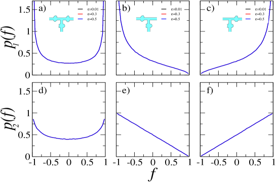
Figure 2: Distribution of $f$ for a chaotic three terminal device for different values of $\varepsilon$ and configurations (insets), (a), (b) and (c) in the presence, and (d), (e) and (f) in the absence, of time reversal invariance.

IV.2 Absence of time reversal invariance

The scattering matrix $S_{j}$ for the $\beta=2$ symmetry has the following parametrization MelloLesHouches ,

$$S_{j}=\left(\begin{array}[]{cc}e^{i\phi_{j}}&0\\ 0&e^{i\psi_{j}}\end{array}\right)\left(\begin{array}[]{cc}-\sqrt{1-\tau_{j}}&\sqrt{\tau_{j}}\\ \sqrt{\tau_{j}}&\sqrt{1-\tau_{j}}\end{array}\right)\left(\begin{array}[]{cc}e^{i\phi^{\prime}_{j}}&0\\ 0&e^{i\psi^{\prime}_{j}}\end{array}\right).$$ (16)

Here, the probability distribution of $S_{j}$ is given by MelloLesHouches

$$dP_{2}(S_{j})=d\tau_{j}\frac{d\phi_{j}}{2\pi}\frac{d\psi_{j}}{2\pi}\frac{d\phi^{\prime}_{j}}{2\pi}\frac{d\psi^{\prime}_{j}}{2\pi},$$ (17)

which defines the Circular Unitary Ensemble.

In Fig. 2, panels (d), (e) and (f), we show the results for the distribution of $f$ for the same values of $\varepsilon$ and configurations as in the $\beta=1$ case. The dependence on the intensity of the coupling, as well as in the position of the probe, is also observed. As in the $\beta=1$ case, the distribution of $f$ is independent of $\varepsilon$ and has memory with respect to the measurement in the midpoint of the horizontal wire. What is important to note here is that the distribution of $f$ is strongly affected by the broken symmetry of time reversal.

V Conclusions

We studied the voltage drop along a horizontal wire with one open mode, consisting of chaotic conductors, in a three terminal device. This was done by using a probe which is chaotic. Our analysis was based on random matrix theory simulations for the chaotic elements, in the presence and absence of time reversal invariance. We found a clear dependence of the position of the probe in the horizontal wire. Also, we found a strong dependence of the time reversal symmetry.

- (1) S. Datta, Electronic Transport in Mesoscopic Systems, Cambridge University Press, Cambridge, 1995.
- (2) S. Goodnick, IEEE Transactions on Nanotechnology 2, 368 (2003).
- (3) R. de Picciotto, H. L. Stormer, L. N. Pfeiffer, K. W. Baldwin, and K. W. West, Nature 411, 51 (2001).
- (4) A. M. Chang, Nature 411, 39 (2001).
- (5) R. Fleischmann and T. Geisel, Phys. Rev. Lett. 89, 016804 (2002).
- (6) S. de Haan, A. Lorke, J. P. Kotthaus, W. Wegscheider, and M. Bichler, Phys. Rev. Lett. 92, 056806 (2004).
- (7) B. Gao, Y. F. Chen, M. S. Fuhrer, D. C. Glattli, and A. Bachtold Phys. Rev. Lett. 95, 196802 (2005).
- (8) H. Aita, L. Arrachea, and C. Naom, Physica B-Condensed Matter 47, 3158 (2012).
- (9) M. Büttiker, Y. Imry, and Y. Azbel, Phys. Rev. A 30, 1982 (1984).
- (10) M. Büttiker, Phys. Rev. Lett. 57, 1761 (1986).
- (11) M. Büttiker, IBM J. Res. Dev. 32, 317 (1988).
- (12) S. Godoy and P. A. Mello, Europhys. Lett. 17, 243 (1992).
- (13) S. Godoy and P. A. Mello, Phys. Rev. B 46, 2346 (1992).
- (14) V. A. Gopar, M. Martínez, and P. A. Mello, Phys. Rev. B 50, 2502 (1994).
- (15) A. M. Song, A. Lorke, A. Kriele, J. P. Kotthaus, W. Wegscheider, and M. Bichler, Phys. Rev. Lett. 80, 3831 (1998).
- (16) A. M. Song, Phys. Rev. B 59, 9806 (1999).
- (17) P. A. Mello, Theory of Random Matrices: Spectral Statistics and Scattering Problems in Mesoscopic Quantum Physics, edited by E. Akkermans, G. Montambaux, J.-L. Pichard, and J. Zinn-Justinm, Elsevier, Amsterdam, 1995.
- (18) C. W. J. Beenakker, Rev. Mod. Phys. 69, 731 (1997).
- (19) Y. Alhassid, Rev. Mod. Phys. 72, 895 (2000).
- (20) F. J. Dyson, J. Math. Phys. 3, 140 (1962).