Heegaard Diagrams Corresponding to Turaev Surfaces

Abstract.

We describe a correspondence between Turaev surfaces of link diagrams on $S^{2}\subset S^{3}$ and special Heegaard diagrams for $S^{3}$ adapted to links.

1. Introduction

To construct the Turaev surface $\Sigma$ of a link diagram $D$ on $S^{2}\subset S^{3}$, one pushes the all-A and all-B states of $D$ to opposite sides of $S^{2}$, connects these two states with a certain cobordism, and caps the state circles with disks. Turaev’s original construction [19] streamlined Murasugi’s proof [16], based on Kauffman’s work  [12] on the Jones polynomial [11], of Tait’s longstanding conjecture on the crossing numbers of alternating links [17]. See also [18]. More recently, Turaev surfaces have provided geometric means for interpreting Khovanov and knot Floer homologies, as in [3, 5, 6, 9, 10, 14, 20].

Dasbach, Futer, Kalfagianni, Lin, and Stoltzfus showed that the Turaev surface of any connected link diagram $D$ on $S^{2}\subset S^{3}$ is a splitting surface for $S^{3}$ on which $D$ forms an alternating link diagram [8]. When equipped with the type of crossing ball structure developed by Menasco [15], the projection sphere provides natural attaching circles for the two handlebodies of this splitting, completing a Heegaard diagram $(\Sigma,\alpha,\beta)$ for $S^{3}$. By characterizing the interplay between this Heegaard diagram and the original link diagram $D$, we obtain a correspondence between Turaev surfaces and particular Heegaard diagrams adapted to links. Figure 1 shows a typical example of such a diagram $(\Sigma,\alpha,\beta,D)$.

First, §2 defines Heegaard splittings and diagrams, link diagrams, crossing ball structures, and Turaev surfaces. Next, §3 constructs and describes the special, link-adapted Heegaard diagrams $(\Sigma,\alpha,\beta,D)$. Finally, §4 establishes the following correspondences:

Theorem 4.1. There is a 1-to-1 correspondence between Turaev surfaces of connected link diagrams on $S^{2}\subset S^{3}$ and diagrams $(\Sigma,\alpha,\beta,D)$ with the following properties:

$\bullet$ $(\Sigma,\alpha,\beta)$ is a Heegaard diagram for $S^{3}$, with $\alpha\pitchfork\beta$.

$\bullet$ $D$ is an alternating link diagram on $\Sigma$ which cuts $\Sigma$ into disks, with $D\pitchfork\alpha$ and $D\pitchfork\beta$.

$\bullet$ $D\cap\alpha=D\cap\beta=\alpha\cap\beta$, none of these points being crossings of $D$.

$\bullet$ There is a checkerboard partition $\Sigma\setminus(\alpha\cup\beta)=\Sigma_{\varnothing}\cup\Sigma_{K}$, in which $\Sigma_{\varnothing}$ consists of disks disjoint from $D$, in which $D$ cuts $\Sigma_{K}$ into disks each of whose boundary contains at least one crossing point and at most two points of $\alpha\cap\beta$, and in which $2g(\Sigma)+|\Sigma_{\varnothing}|=|\alpha|+|\beta|$.

Theorem 4.2: There is a 1-to-1 correspondence between generalized Turaev surfaces, constructed from dual pairs of states of connected link diagrams on $S^{2}\subset S^{3}$, and diagrams $(\Sigma,\alpha,\beta,D)$ with the properties in Theorem 4.1, except that $D$ need not alternate on $\Sigma$.

      

Figure 1. A link diagram on $S^{2}$, and the link-adapted Heegaard diagram $(\Sigma,\alpha,\beta,D)$ corresponding to its Turaev surface, the torus in Figure 7. As in all figures, the link is black; the crossing balls are white; the attaching circles comprising $\alpha$ and $\beta$ are red and blue, respectively; and the circles and disks from the all-A state are green, while those from the all-B state are brown.

Acknowledgements: We would like to thank Charlie Frohman, Maggy Tomova, Ryan Blair, Oliver Dasbach, Adam Lowrance, Neal Stoltzfus, and Effie Kalfagianni for helpful conversations.

2. Background

2.1. Heegaard splittings and diagrams

A Heegaard splitting of an orientable $3$-manifold $M$ is a decomposition of $M$ into two handlebodies $H_{\alpha}$ and $H_{\beta}$ with common boundary. The surface $\partial H_{\alpha}=\partial H_{\beta}=\Sigma$ is called a splitting surface for $M$. In this paper, we address only the case in which $M=S^{3}$.

One can describe a handlebody $H$ by identifying on its boundary $\partial H=\Sigma$ a collection of disjoint, simple closed curves $\alpha_{1},\ldots,\alpha_{k}$, such that each $\alpha_{i}$ bounds a disk $\hat{\alpha}_{i}$ in $H$, and such that these disks together cut $H$ into a disjoint union of balls. The $\alpha_{i}$ are called attaching circles for $H$. Some conventions require that the $\hat{\alpha}_{i}$ together cut $H$ into a single ball, hence $k=g(\Sigma)$; though not requiring this, our definition does imply that $k\geq g(\Sigma)$.

A Heegaard diagram $(\Sigma,\alpha,\beta)$ combines these ideas to blueprint a 3-manifold. The diagram consists of a splitting surface $\Sigma=\partial H_{\alpha}=\partial H_{\beta}$, together with a union ${\alpha}=\bigcup\alpha_{i}$ of attaching circles for $H_{\alpha}$ and a union ${\beta}=\bigcup\beta_{i}$ of attaching circles for $H_{\beta}$. If $(\Sigma,\alpha,\beta)$ is a Heegaard diagram for $S^{3}$, then the circles of $\alpha$ and $\beta$ together generate $H_{1}(\Sigma)$. The Appendix provides an easy proof of this fact, using Seifert surfaces.

Figure 2. Each crossing in a link diagram is labeled in one of two ways. The label tells one how to adjust the link after inserting a crossing ball.

2.2. Link diagrams and crossing balls

A link diagram $D$ on a closed surface $F\subset S^{3}$ is the image, in general position, of an immersion of one or more circles in $F$; each arc at any crossing point is labeled with a direction normal to $F$ near that point, so that under- and over-crossings have been identified. By inserting small, mutually disjoint crossing balls $C=\bigcup C_{i}$ centered at the crossing points of $D$ and pushing the two intersecting arcs of each $D\cap C_{i}$ off $F$ to the appropriate hemisphere of $\partial C_{i}\setminus F$, as in Figure 2, one obtains a configuration of a link $K\subset(F\setminus C)\cup\partial C\subset S^{3}$. Call this a crossing ball configuration of the link $K$ corresponding to the link diagram $D$.

Conversely, given mutually disjoint crossing balls $C=\bigcup C_{i}$ centered at points on a closed surface $F\subset S^{3}$, and a link $K\subset(F\setminus C)\cup\partial C$ in which each crossing ball appears as in Figure 2, one may obtain a corresponding link diagram as follows. Consider a regular neighborhood of $F$ that contains $C$ and is parameterized by an orientation-preserving homeomorphism with $F\times[-1,1]$ which identifies $F$ with $F\times\{0\}$. If $\pi:F\times[-1,1]\to F$ denotes the natural projection, the link diagram corresponding to the crossing ball configuration $K\subset(F\setminus C)\cup\partial C\subset S^{3}$ is the projected image $\pi(K)\subset F$ with appropriate crossing labels.

In such a crossing ball configuration, each arc of $K\cap\partial C$ lies either in $F\times[-1,0]$ or in $F\times[0,1]$. The former arcs are called under-passes, and the latter are called over-passes. A link diagram $D$ is said to be alternating if each arc of $K\setminus C$ in a corresponding crossing ball configuration joins an under-pass with an over-pass. A link $K\subset S^{3}$ is alternating if it has an alternating diagram on $S^{2}$.

In particular, any Heegaard diagram $(\Sigma,\alpha,\beta)$ for $S^{3}$ provides an embedding of the closed surface $\Sigma$ in $S^{3}$. One may therefore superimpose a link diagram $D$ on the Heegaard diagram to obtain a new type of diagram $(\Sigma,\alpha,\beta,D)$. This new diagram describes a Heegaard splitting of $S^{3}$ in which the splitting surface contains a link diagram.

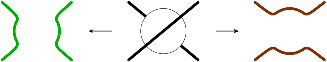
Figure 3. The A-smoothing (left) and B-smoothing (right) of a crossing.

2.3. Turaev surfaces

Each crossing in a link diagram $D$ on a surface $F$ can be smoothed in two different ways, by inserting a crossing ball $C_{i}$ and replacing $D\cap C_{i}$ with one of the two pairs of arcs of $(\partial C_{i}\cap F)\setminus D$ opposite to another. Figure 3 shows the two possibilities, called the A-smoothing and the B-smoothing of the crossing. Making a choice of smoothing for each crossing in the diagram produces a disjoint union of circles on $F$, called a state of the diagram $D$. Two states of $D$ are dual if they have opposite smoothings at each crossing.

Figure 4. The all-A (left) and all-B (right) states for a link diagram.

Given a link diagram $D$ on $S^{2}$, the two extreme states – the all-A and the all-B – are of particular interest, due in part to the bounds they give on the maximum and minimum degrees of the Jones polynomial. Kauffman’s proof [12] that these bounds are sharp for reduced, alternating diagrams provided the impetus for Murasugi [16], Thistlethwaite [18], and Turaev [19] to prove Tait’s conjecture on the crossing numbers of alternating links. Cromwell [7], Lickorish and Thistlethwaite [13] then extended these results to adequate link diagrams. Figure 4 shows the all-A and all-B states for the link diagram from Figure 1.

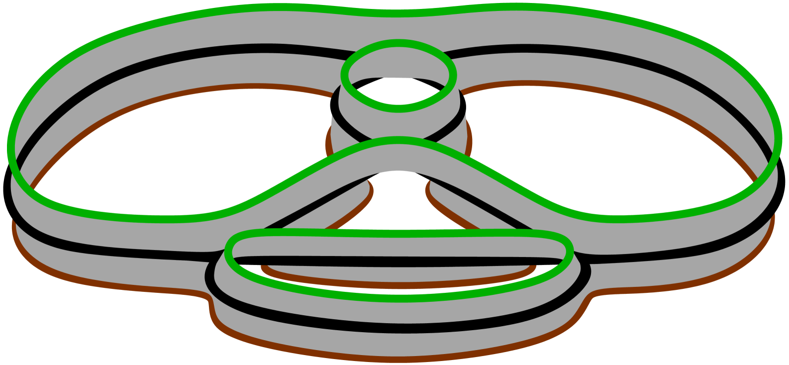
Figure 5. The cobordism between the all-A and all-B states from Figure 4.

Following Turaev [19], one can construct a cobordism between the all-A and all-B states as follows. Parameterize a bi-collaring of $S^{2}$ as in §2.2, and push the all-A and all-B states off $S^{2}$ to $S^{2}\times\{1\}$ and $S^{2}\times\{-1\}$, respectively, such that each state circle sweeps out an annulus to one side of $S^{2}$. Assume that these annuli are mutually disjoint, and that they are disjoint from the crossing balls $C=\bigcup C_{i}$ used to construct the all-A and all-B states. Gluing together these annuli and the disks of $S^{2}\cap C$ produces the cobordism between the two states. (See Figure 5.) Near each crossing, the cobordism has a saddle, as in Figure 6.

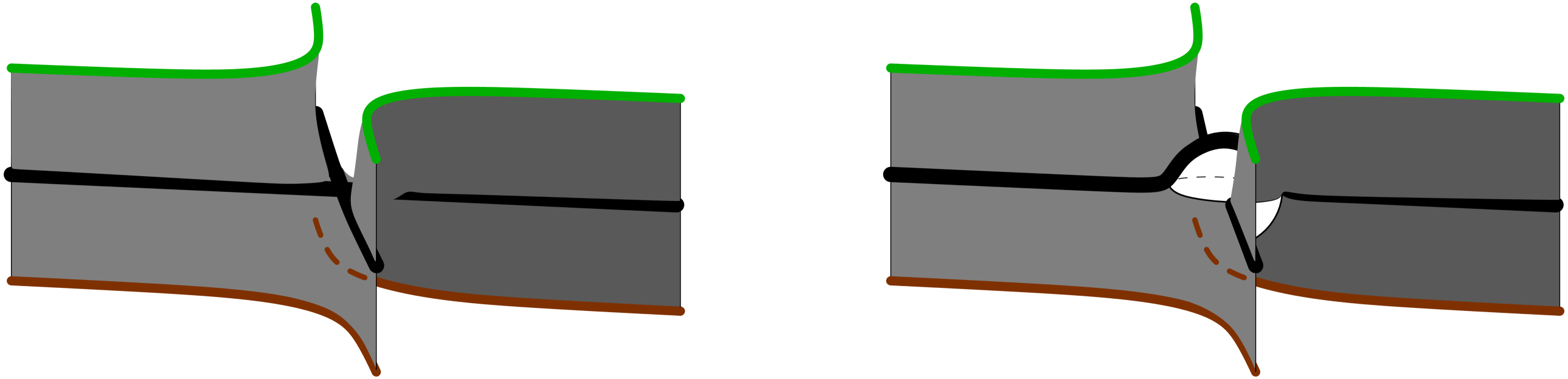
Figure 6. Turaev’s cobordism between the all-A and all-B states has a saddle near each crossing, shown here with and without a crossing ball.

Having constructed the cobordism, one caps the all-A and all-B states with mutually disjoint disks to form a closed surface $\Sigma$, called the Turaev surface of the original link diagram $D$ on $S^{2}$. Since $\Sigma$ contains a neighborhood of $S^{2}$ around each crossing point, the crossing information of $D$ on $S^{2}$ translates to crossing information on the Turaev surface. Thus, $D$ forms a link diagram on $\Sigma$. A crossing ball configuration corresponding to this link diagram is $K\subset(\Sigma\setminus C)\cup\partial C$, with under- and over-passes defined as in §2.2.

Figure 7. This torus is the Turaev surface of the link diagram in Figures 1 and 4, seen from the ambient space. To provide a window to the far side of the surface, one of the three disks of the all-A state is only partly shown.

Observe that $D$ cuts $\Sigma$ into disks, each of which contains exactly one state disk, and that $S^{2}\cap\Sigma=S^{2}\cap(C\cup K)=\Sigma\cap(C\cup K)$. Note also that if $D$ is alternating on $S^{2}$, then $\Sigma$ is a sphere which can be isotoped to $S^{2}$ while fixing $D$. Figure 7 shows a less trivial example.

The construction of the Turaev surface generalizes to any pair of states $s$ and $\tilde{s}$ dual to one another. By pushing $s$ and $\tilde{s}$ to opposite sides of $S^{2}$ to sweep out annuli on opposite sides of $S^{2}$, gluing in disks near the crossings to obtain a cobordism between $s$ and $\tilde{s}$, and capping off with disks, one obtains a closed surface $\Sigma$ on which $D$ forms a link diagram [1, 19]. Call this surface $\Sigma$ the generalized Turaev surface of the dual states $s$ and $\tilde{s}$.

3. Construction of Heegaard diagrams for Turaev surfaces

Given a connected link diagram $D$ on $S^{2}\subset S^{3}$ and its Turaev surface $\Sigma$, this section constructs a link-adapted Heegaard diagram $(\Sigma,\alpha,\beta,D)$. Theorem 3.4 then characterizes this diagram, providing one direction of the correspondence to come in Theorem 4.1.

Let $K\subset(S^{2}\setminus C)\cup\partial C$ be a crossing ball structure corresponding to $D$, and let $H_{\alpha}$ and $H_{\beta}$ be the two components of $S^{3}\setminus\Sigma$. Define $\hat{\alpha}:=(S^{2}\setminus(C\cup K))\cap H_{\alpha}$ and $\hat{\beta}:=(S^{2}\setminus(C\cup K))\cap H_{\beta}$ to be the two checkerboard classes of $S^{2}\setminus(C\cup K)$, with $\alpha:=\partial\hat{\alpha}$ and $\beta:=\partial\hat{\beta}$. From this setup, three modifications will complete the construction of the diagram $(\Sigma,\alpha,\beta,D)$. During these changes, $\Sigma$, $D$, $S^{2}$, $C$, and $K$ will remain fixed.

First, perturb $\alpha$ and $\beta$ through the cobordism as follows, carrying along the disks of $\hat{\alpha}$ and $\hat{\beta}$. Let $X=\{x_{1},\ldots,x_{n}\}$ consist of one point on each arc of $K\setminus C$ which joins two under-passes on $S^{2}$, and let $Y=\{y_{1},\ldots,y_{n}\}$ consist of one point on each arc of $K\setminus C$ which joins two over-passes on $S^{2}$. Each arc of ${\alpha}\setminus(X\cup Y)$ runs along a circle from either the all-A state or the all-B state. Isotope ${\alpha}$ through the cobordism so as to push arcs of the former type to $S^{2}\times(0,1)$ and arcs of the latter type to $S^{2}\times(-1,0)$, giving $\alpha\cap C=\varnothing$ and ${\alpha}\cap D=X\cup Y$. Next, isotope ${\beta}$ in the same manner, after which $\alpha$ and $\beta$ will both be disjoint from $C$, while $\alpha$, $\beta$, and $D$ will be pairwise transverse and will intersect exclusively at triple points: ${\alpha}\cap{\beta}={\alpha}\cap D={\beta}\cap D=X\cup Y$.

To further simplify the picture, push the state circles through the cobordism to align with $\alpha\cup\beta$, so that each state disk becomes a component of $\Sigma\setminus(\alpha\cup\beta)$. This causes the neighborhood of each arc of $K\setminus C$ to appear as in Figure 8, possibly with red and blue reversed. Note that the state disks’ interiors remain disjoint from $D$, in fact from $S^{2}$.

To complete the construction, remove any attaching circles that are disjoint from $D$. Also remove the corresponding disks of $\hat{\alpha}$ and $\hat{\beta}$, and let $\alpha$, $\beta$, $\hat{\alpha}$ and $\hat{\beta}$ retain their names. Because each removed circle lies in some disk of $\Sigma\setminus D$, each removed disk is parallel to $\Sigma$.

Lemma 3.1 (DFKLS [8]).

The Turaev surface $\Sigma$ of any connected link diagram $D$ on $S^{2}\subset S^{3}$ is a splitting surface for $S^{3}$.

Proof.

Observe that $S^{2}\cup C$ cuts $S^{3}$ into two balls, which $\Sigma$ cuts into smaller balls. Also, $S^{3}\setminus(S^{2}\cup C\cup\Sigma)=(H_{\alpha}\setminus(S^{2}\cup C))\cup(H_{\beta}\setminus(S^{2}\cup C))$, where $H_{\alpha}$ and $H_{\beta}$ are the two components of $S^{3}\setminus\Sigma$. Hence, $H_{\alpha}\setminus C$ and $H_{\beta}\setminus C$ are handlebodies, as are $H_{\alpha}$ and $H_{\beta}$. ∎

The proof of Lemma 3.1 implies that $(\Sigma,\alpha,\beta)$ was a Heegaard diagram for $S^{3}$ when $\alpha$ and $\beta$ were first defined. The fact that each removed disk of $\hat{\alpha}$ and of $\hat{\beta}$ was parallel to $\Sigma$ implies that $(\Sigma,\alpha,\beta)$ is a Heegaard diagram for $S^{3}$ in the finished construction as well.

Figure 8. Up to reversing red and blue, these are the possible configurations of the Turaev surface $\Sigma$ between two adjacent crossings, shown at the stage of the construction in which the boundary of each state disk lies in $\alpha\cup\beta$.

Lemma 3.2 (DFKLS [8]).

Any connected link diagram $D$ on $S^{2}\subset S^{3}$ forms an alternating link diagram on its Turaev surface $\Sigma$.

Proof.

Recall from §2.3 that $D$ forms a link diagram on $\Sigma$. On $S^{2}$, each arc $\kappa$ of $K\setminus C$ joins either two over-passes, two under-passes, or one of each. Figure 8 shows the three possible configurations of $\Sigma$ near $\kappa$, prior to the removal of attaching circles, up to reversal of $\alpha$ and $\beta$. In all three cases, the two arcs of $K\cap\partial C$ incident to $\kappa$ lie to opposite sides of $\Sigma$, so that one is an over-pass on $\Sigma$ and the other is an under-pass on $\Sigma$. ∎

One defines the Turaev genus $g_{T}(K)$ of a link $K\subset S^{3}$ to be the minimum genus among the Turaev surfaces of all diagrams of $K$ on $S^{2}$. The resulting invariant, surveyed in [4], measures how far a link is from being alternating. See also [2]. In particular, Turaev genus provides the crux of Turaev’s proof of Tait’s conjecture:

Corollary 3.3 (Turaev [19], DFKLS [8]).

A link $K$ is alternating if and only if $g_{T}(K)=0$.

Theorem 3.4.

From the Turaev surface $\Sigma$ of a connected link diagram $D$ on $S^{2}\subset S^{3}$, the construction in this section produces a diagram $(\Sigma,\alpha,\beta,D)$ with the following properties:

$\bullet$ $(\Sigma,\alpha,\beta)$ is a Heegaard diagram for $S^{3}$, with $\alpha\pitchfork\beta$.

$\bullet$ $D$ is an alternating link diagram on $\Sigma$ which cuts $\Sigma$ into disks, with $D\pitchfork\alpha$ and $D\pitchfork\beta$.

$\bullet$ $D\cap\alpha=D\cap\beta=\alpha\cap\beta$, none of these points being crossings of $D$.

$\bullet$ There is a checkerboard partition $\Sigma\setminus(\alpha\cup\beta)=\Sigma_{\varnothing}\cup\Sigma_{K}$, in which $\Sigma_{\varnothing}$ consists of disks disjoint from $D$, in which $D$ cuts $\Sigma_{K}$ into disks each of whose boundary contains at least one crossing point and at most two points of $\alpha\cap\beta$, and in which $2g(\Sigma)+|\Sigma_{\varnothing}|=|\alpha|+|\beta|$.

Proof.

We have already established the first three properties. Let $\Sigma_{\varnothing}$ consist of the interiors of all adjusted state disks whose boundary contains at least one point of $\alpha\cap\beta$, i.e. those whose boundary still lies in $\alpha\cup\beta$ after the removal of the attaching circles disjoint from $D$. These state disks are disjoint from $D$ and constitute a checkerboard class of $\Sigma\setminus(\alpha\cup\beta)$. See Figure 9.

Let $\Sigma_{K}$ denote the other checkerboard class of $\Sigma\setminus(\alpha\cup\beta)$. Each component of $\Sigma_{K}\setminus D$ is also a component of $(\Sigma\setminus D)\setminus(\alpha\cup\beta)$, and each attaching circle intersects $D$; therefore, $D$ cuts $\Sigma_{K}$ into disks. Further, each arc of $K\setminus C$ contains at most one point of $\alpha\cap\beta$, and each arc of $(\alpha\cup\beta)\setminus D$ is parallel through $\Sigma$ to $D$; consequently, the boundary of each disk of $\Sigma_{K}\setminus D$ contains at least one crossing point and at most one arc of $(\alpha\cup\beta)\setminus D$, hence at most two points of $\alpha\cap\beta$.

Finally, to see that $2g(\Sigma)+|\Sigma_{\varnothing}|=|\alpha|+|\beta|$, consider Euler characteristic in light of the observation that removing the disks of $\Sigma_{\varnothing}$ from $\Sigma$ and gluing in the disks of $\hat{\alpha}$ and $\hat{\beta}$ yields a sphere isotopic to $S^{2}$. Near each point of $\alpha\cap\beta$, this surgery appears as in Figure 9. ∎

Figure 9. Given a diagram $(\Sigma,\alpha,\beta,D)$ with the properties in Theorems 3.4, 4.1, or 4.2, removing the disks of $\Sigma_{\varnothing}$ from $\Sigma$ and gluing in the disks of $\hat{\alpha}$ and $\hat{\beta}$ produces a sphere on which $D$ forms a link diagram. Near each point of $\alpha\cap\beta$, this surgery appears as shown, up to mirroring.

4. Correspondence between Heegaard diagrams and Turaev surfaces

4.1. Main correspondence

From the Turaev surface of a connected link diagram on $S^{2}\subset S^{3}$, we have constructed a link-adapted Heegaard diagram $(\Sigma,\alpha,\beta,D)$ with several properties. We will now see that any such diagram corresponds to the Turaev surface of some link diagram on the sphere.

Theorem 4.1.

There is a 1-to-1 correspondence between Turaev surfaces of connected link diagrams on $S^{2}\subset S^{3}$ and diagrams $(\Sigma,\alpha,\beta,D)$ with the following properties:

$\bullet$ $(\Sigma,\alpha,\beta)$ is a Heegaard diagram for $S^{3}$, with $\alpha\pitchfork\beta$.

$\bullet$ $D$ is an alternating link diagram on $\Sigma$ which cuts $\Sigma$ into disks, with $D\pitchfork\alpha$ and $D\pitchfork\beta$.

$\bullet$ $D\cap\alpha=D\cap\beta=\alpha\cap\beta$, none of these points being crossings of $D$.

$\bullet$ There is a checkerboard partition $\Sigma\setminus(\alpha\cup\beta)=\Sigma_{\varnothing}\cup\Sigma_{K}$, in which $\Sigma_{\varnothing}$ consists of disks disjoint from $D$, in which $D$ cuts $\Sigma_{K}$ into disks each of whose boundary contains at least one crossing point and at most two points of $\alpha\cap\beta$, and in which $2g(\Sigma)+|\Sigma_{\varnothing}|=|\alpha|+|\beta|$.

Proof.

Theorem 3.4 provides one direction of this correspondence. It remains to prove the converse.

Assume that the diagram $(\Sigma,\alpha,\beta,D)$ is as described. Remove the disks of $\Sigma_{\varnothing}$ from $\Sigma$ and glue in the disks of $\hat{\alpha}$ and $\hat{\beta}$ to obtain a closed surface. (See Figure 9.) Because $D$ is connected and $2g(\Sigma)+|\Sigma_{\varnothing}|=|\alpha|+|\beta|$, this surface is a sphere – call it $S^{2}$. Moreover, $D$, being disjoint from $\Sigma_{\varnothing}$ and having its crossing points in $\Sigma_{K}$, forms a link diagram on $S^{2}$. We claim, up to isotopy, that $\Sigma$ is the Turaev surface of the link diagram $D$ on $S^{2}$.

The property that $D$ cuts $\Sigma_{K}$ into disks implies that $D$ intersects each attaching circle, cutting $\alpha$ and $\beta$ into arcs. Because the boundary of each disk of $\Sigma_{K}\setminus D$ contains at most two points of $\alpha\cap\beta$, each of these arcs is parallel through one of these disks to $D$. The property that the boundary of each disk of $\Sigma_{K}\setminus D$ contains at least one crossing point then implies that there is at most one point of $\alpha\cap\beta$ on $D$ between any two adjacent crossings.

The link diagram $D$ cuts $S^{2}$ into disks admitting a checkerboard partition. Because $S^{2}$ appears near each point of $\alpha\cap\beta$ as in Figure 9, one of the checkerboard classes contains $\hat{\alpha}$, and the other contains $\hat{\beta}$. Yet, some disks of $S^{2}\setminus D$ may be entirely contained in $\Sigma_{K}$, hence disjoint from $\alpha$ and $\beta$. Construct an attaching circle in the interior of each such disk, and incorporate it into either $\alpha$ or $\beta$ according to the checkerboard pattern, letting $\alpha$ and $\beta$ retain their names. Span each new circle of $\alpha$ by a new disk of $\hat{\alpha}$ on the same side of $\Sigma$ as the other disks of $\hat{\alpha}$, and similarly span each new circle of $\beta$ by a new disk of $\hat{\beta}$.

The components of $\Sigma\setminus(\alpha\cup\beta)$ still admit a checkerboard partition, $\Sigma\setminus(\alpha\cup\beta)=\Sigma_{\varnothing}\cup\Sigma_{K}$, in which $\Sigma_{\varnothing}$ consists of disks disjoint from $D$, though $D$ no longer need cut $\Sigma_{K}$ into disks. The preceding modification of $\alpha$, $\beta$, $\hat{\alpha}$, and $\hat{\beta}$ corresponds to an isotopy of $S^{2}$, which again may be obtained from $\Sigma$ by removing the disks of $\Sigma_{\varnothing}$ and gluing in the disks of $\hat{\alpha}$ and $\hat{\beta}$.

Let $K\subset(\Sigma\setminus C)\cup\partial C$ be a crossing ball configuration corresponding to the link diagram $D$ on $\Sigma$, with $C\cap\alpha=\varnothing=C\cap\beta$. Note that $K\subset(S^{2}\setminus C)\cup\partial C$ is also a crossing ball configuration corresponding to the link diagram $D$ on $S^{2}$.

Currently $\Sigma$ and $S^{2}$ are non-transverse, even away from $C$, as both $\Sigma$ and $S^{2}$ contain $\Sigma_{K}$. Rectify this by perturbing $S^{2}$ as follows, fixing $\Sigma$, $\alpha$, $\beta$, $\hat{\alpha}$, $\hat{\beta}$, $D$, $\Sigma_{\varnothing}$, $\Sigma_{K}$, $C$, and $K$ in the process. (We initially constructed $S^{2}$ by gluing together $\hat{\alpha}$, $\hat{\beta}$, and $\Sigma_{K}$, but now we are pushing $S^{2}$ off of them.) Each disk of $S^{2}\setminus(C\cup K)$ currently contains a disk of either $\hat{\alpha}$ or $\hat{\beta}$; push the disk of $S^{2}\setminus(C\cup K)$ off $\Sigma$ in the corresponding direction, while fixing its boundary, which lies in $\Sigma\cap(K\cup\partial C)$. This isotopy makes $S^{2}$ disjoint from $\alpha$ and $\beta$, except at the points of $\alpha\cap\beta$. In fact, this isotopy gives $S^{2}\cap\Sigma=S^{2}\cap(C\cup K)=\Sigma\cap(C\cup K)$, as was the case in §2.3. (Recall Figure 6.)

Because $D$ is alternating on $\Sigma$, the disks of $\Sigma\setminus(C\cup K)$ admit a checkerboard partition – the boundaries of the disks in the two classes are the all-A and all-B state circles for the link diagram $D$ on $\Sigma$. Further, each of these state circles on $\Sigma$ encloses precisely one disk of $\Sigma_{\varnothing}$. Color green each disk of $\Sigma_{\varnothing}$ enclosed by a circle from the all-A state, and color brown each disk of $\Sigma_{\varnothing}$ enclosed by a circle from the all-B state. Near each arc of $K\setminus C$, $\Sigma$ now appears as in Figure 8 (possibly with red and blue reversed). As a final adjustment, slightly perturb the green and brown disks so that they become disjoint from $\alpha$, $\beta$, and $D$.

Removing the green and brown disks from $\Sigma$ leaves a cobordism between their boundaries. Cutting this cobordism along $S^{2}\cap(K\cup\partial C)$ yields the disks of $S^{2}\setminus C$, together with annuli lying to either side of $S^{2}$, through which the boundaries of the green and brown disks are respectively parallel to the all-A and all-B states of the link diagram $D$ on $S^{2}$. As claimed, $\Sigma$ is therefore the Turaev surface of the link diagram $D$ on $S^{2}$. ∎

4.2. Generalization to arbitrary dual states

As noted at the end of §2.3, the construction of the Turaev surface from the all-A and all-B states of a link diagram $D$ on $S^{2}$ generalizes to any pair of states of $D$ which are dual to one another, having opposite smoothings at each crossing. The correspondence developed in §3 and §4.1 between link-adapted Heegaard diagrams $(\Sigma,\alpha,\beta,D)$ and Turaev surfaces extends to these generalized Turaev surfaces, the only difference being that $D$ no longer need alternate on $\Sigma$.

Theorem 4.2.

There is a 1-to-1 correspondence between generalized Turaev surfaces of connected link diagrams on $S^{2}\subset S^{3}$, and diagrams $(\Sigma,\alpha,\beta,D)$ with the following properties:

$\bullet$ $(\Sigma,\alpha,\beta)$ is a Heegaard diagram for $S^{3}$, with $\alpha\pitchfork\beta$.

$\bullet$ $D$ is a link diagram on $\Sigma$ which cuts $\Sigma$ into disks, with $D\pitchfork\alpha$ and $D\pitchfork\beta$.

$\bullet$ $D\cap\alpha=D\cap\beta=\alpha\cap\beta$, none of these points being crossings of $D$.

$\bullet$ There is a checkerboard partition $\Sigma\setminus(\alpha\cup\beta)=\Sigma_{\varnothing}\cup\Sigma_{K}$, in which $\Sigma_{\varnothing}$ consists of disks disjoint from $D$, in which $D$ cuts $\Sigma_{K}$ into disks each of whose boundary contains at least one crossing point and at most two points of $\alpha\cap\beta$, and in which $2g(\Sigma)+|\Sigma_{\varnothing}|=|\alpha|+|\beta|$.

Proof.

Given the generalized Turaev surface $\Sigma$ for dual states $s$ and $\tilde{s}$ of a connected link diagram $D$ on $S^{2}\subset S^{3}$, reverse some collection of the crossings of $D$ to obtain a new link diagram $D^{\prime}$ for which $s$ and $\tilde{s}$ are the all-A and all-B states. Construct the corresponding diagram $(\Sigma,\alpha,\beta,D^{\prime})$ as in §3. Finally, switch back the reversed crossings of $D^{\prime}$ to obtain the required diagram $(\Sigma,\alpha,\beta,D)$.

Conversely, suppose that $(\Sigma,\alpha,\beta,D)$ is as described. The proof of Theorem 4.1 extends almost verbatim. The only concern, as $D$ need not alternate on $\Sigma$, is whether or not the disks of $\Sigma\setminus D$ admit a checkerboard partition; it suffices to show that they do.

The condition that $D\cap\Sigma_{\varnothing}=\varnothing$ implies that one endpoint of each arc of $(\alpha\cup\beta)\setminus D$ appears as in Figure 9, and the other appears as the mirror image. Thus, each attaching circle intersects $D$ in an even number of points. The fact that the attaching circles generate $H_{1}(\Sigma)$ then implies that any simple closed curve on $\Sigma$ in general position with respect to $D$ must intersect $D$ in an even number of points, and hence that the disks of $\Sigma\setminus D$ admit a checkerboard partition. ∎

4.3. Conclusion

Up to isotopy, each link diagram on $S^{2}\subset S^{3}$ has a unique Turaev surface. Theorem 4.1 thus establishes – via Turaev surfaces – a 1-to-1 correspondence between link diagrams on $S^{2}\subset S^{3}$ and alternating, link-adapted Heegaard diagrams $(\Sigma,\alpha,\beta,D)$.

Similarly, Theorem 4.2 establishes – via generalized Turaev surfaces constructed from dual states – a 2-to-1 correspondence between states of link diagrams on $S^{2}\subset S^{3}$ and link-adapted Heegaard diagrams $(\Sigma,\alpha,\beta,D)$ for $S^{3}$ in which $D$ need not alternate on $\Sigma$.

5. Appendix

Let $(\Sigma,\alpha,\beta)$ be a Heegaard diagram for $S^{3}$, and let $\gamma\subset\Sigma$ be an oriented, simple closed curve. The following construction yields an expression for $[\gamma]\in H_{1}(\Sigma)$ in terms of the homology classes of the oriented attaching circles, proving that the latter generate $H_{1}(\Sigma)$.

Because $H_{1}(S^{3})$ is trivial, $\gamma$ bounds a Seifert surface $S\subset S^{3}$, on which $\gamma$ induces an orientation. Fixing $\gamma$, isotope $S$ so that its interior intersects $\Sigma$ transversally – along simple closed curves and along arcs with endpoints on $\gamma$.

Given a component $S_{\alpha,i}$ of $S\cap H_{\alpha}$, one may obtain an expression for $[\partial S_{\alpha,i}]\in H_{1}(\Sigma)$ in terms of the $[\alpha_{j}]$ by surgering $S_{\alpha,i}$ along successive outermost disks of $\hat{\alpha}\setminus S_{\alpha,i}$ until $\partial S_{\alpha,i}$ lies entirely in the punctured sphere $\Sigma\setminus\alpha$, at which point the expression is evident. An analogous procedure expresses the homology class of each component of $S\cap H_{\beta}$ in terms of the $[\beta_{j}]$. Summing over all components of $S\setminus\Sigma$ gives the desired expression for $[\gamma]\in H_{1}(\Sigma)$:

$$[\gamma]=[\partial S]=\sum_{\begin{matrix}\small{\text{Components }}\\ \small{S_{\alpha,i}\text{ of }S\cap H_{\alpha}}\\ \end{matrix}}[\partial S_{\alpha,i}]+\sum_{\begin{matrix}\small{\text{Components }}\\ \small{S_{\beta,i}\text{ of }S\cap H_{\beta}}\\ \end{matrix}}[\partial S_{\beta,i}]=\sum_{i,j}a_{i,j}[\alpha_{j}]+\sum_{i,j}b_{i,j}[\beta_{j}]$$

Conversely, if $(\Sigma,\alpha,\beta)$ is a Heegaard diagram for a 3-manifold $M$ with nontrivial first homology, then the oriented attaching circles do not generate $H_{1}(\Sigma)$, since inclusion $\Sigma\hookrightarrow M$ induces a surjective map $H_{1}(\Sigma)\to H_{1}(M)$, whose kernel contains all the $[\alpha_{j}]$ and $[\beta_{j}]$.

References

- [1] Y. Bae, H.R. Morton, The spread and extreme terms of Jones polynomials, J. Knot Theory Ramifications 12 (2003), 359-373.
- [2] C.L.J. Balm, Topics in knot theory: On generalized crossing changes and the additivity of the Turaev genus, Thesis (Ph.D.) – Michigan State University (2013).
- [3] A. Champanerkar, I. Kofman, Spanning trees and Khovanov homology, Proc. Amer. Math. Soc. 137 (2009), no. 6, 2157-2167.
- [4] A. Champanerkar, I. Kofman, A survey on the Turaev genus of knots, arXiv:1406.1945, preprint.
- [5] A. Champanerkar, I. Kofman, N. Stoltzfus, Graphs on surfaces and Khovanov homology, Algebr. and Geom. Topol. 7 (2007), 1531-1540.
- [6] A. Champanerkar, I. Kofman, N. Stoltzfus, Quasi-tree expansion for the Bollobs-Riordan-Tutte polynomial, Bull. Lond. Math. Soc. 43 (2011), no. 5, 972-984.
- [7] P.R. Cromwell, Homogeneous links, J. London Math. Soc. (2) 39 (1989), no. 3, 535-552.
- [8] O.T. Dasbach, D. Futer, E. Kalfagianni, X.-S. Lin, N. Stoltzfus, The Jones polynomial and graphs on surfaces, J. Combin. Theory Ser. B 98 (2008), no. 2, 384-399.
- [9] O.T. Dasbach, A. Lowrance, Turaev genus, knot signature, and the knot homology concordance invariants, Proc. Amer. Math. Soc. 139 (2011), no. 7, 2631-2645.
- [10] O.T. Dasbach, A. Lowrance, A Turaev surface approach to Khovanov homology, arXiv:1107.2344v2.
- [11] V.F.R. Jones, A polynomial invariant for knots via Von Neumann algebras, Bull. Amer. math. Soc. (N.S.) 12 (1985), no. 1, 103-111.
- [12] L.H. Kauffman, State models and the Jones polynomial, Topology 26 (1987), no. 3, 395-407.
- [13] W.B.R. Lickorish and M.B. Thistlethwaite, Some links with non-trivial polynomials and their crossing numbers, Comment. Math. Helv. 63 (1988), no. 4, 527-539.
- [14] A. Lowrance, On knot Floer width and Turaev genus, Algebr. Geom. Topol. 8 (2008), no. 2, 1141-1162.
- [15] W. Menasco, Closed incompressible surfaces in alternating knot and link complements, Topology 23 (1984), no. 1, 37-44.
- [16] K. Murasugi, Jones polynomials and classical conjectures in knot theory, Topology 26 (1987), no. 2, 187-194.
- [17] P.G. Tait, On Knots I, II, and III, Scientific papers 1 (1898), 273-347.
- [18] M.B. Thistlethwaite, A spanning tree expansion of the Jones polynomial, Topology 26 (1987), no. 3, 297-309.
- [19] V.G. Turaev, A simple proof of the Murasugi and Kauffman theorems on alternating links, Enseign. Math. (2) 33 (1987), no. 3-4, 203-225.
- [20] S. Wehrli, A spanning tree model for Khovanov homology, J. Knot Theory Ramifications 17 (2008), no. 12, 1561-1574.