ROTATION OF THE OPTICAL POLARIZATION ANGLE ASSOCIATED WITH THE 2008 $\gamma$-RAY FLARE OF BLAZAR W COMAE

Abstract

An $R$–band photopolarimetric variability analysis of the TeV bright blazar W Comae, between 2008 February 28 and 2013 May 17, is presented. The source showed a gradual tendency to decrease its mean flux level with a total change of  3 mJy. A maximum and minimum brightness states in the $R$-band of 14.25$\pm$0.04 and 16.52$\pm$0.1 mag respectively were observed, corresponding to a maximum variation of $\Delta$F = 5.40 mJy. We estimated a minimum variability timescale of $\Delta$t=3.3 days. A maximum polarization degree $P$=33.8%$\pm$1.6%, with a maximum variation of $\Delta$P = 33.2%, was found. One of our main results is the detection of a large rotation of the polarization angle from 78°to 315°($\Delta\theta\sim$237°) that coincides in time with the $\gamma$-ray flare observed in 2008 June. This result indicates that both optical and $\gamma$-ray emission regions could be co-spatial. During this flare, a correlation between the $R$-band flux and polarization degree was found with a correlation coefficient of $r_{F-p}=0.93\pm$0.11. From the Stokes parameters we infer the existence of two optically thin synchrotron components that contribute to the polarized flux. One of them is stable with a constant polarization degree of 11%. Assuming a shock-in jet model during the 2008 flare, we estimated a maximum Doppler factor $\delta_{D}\sim 27$ and a minimum of $\delta_{D}\sim 16$; a minimum viewing angle of the jet $\sim$2°.0; and a magnetic field $B\sim$ 0.12 G.

1 INTRODUCTION

The study of the Blazar phenomenon has been one of the major topics of study on the Active Galactic Nuclei (AGN) family because of their extreme properties. They show strong flux variability, superluminal motion, and a non-thermal continuum extending from radio to TeV $\gamma$–ray regions (e.g., Jorstad et al., 2005; Abdo et al., 2010b; Marscher et al., 2010; Agudo et al., 2013). Blazars are radio–loud AGN and consist of BL Lacertae objects and Flat Spectrum Radio Sources (FSRQ; Angel & Stockman, 1980; Fossati et al., 1997; Agudo et al., 2010; Costamante, 2012). These properties are explained through the idea that blazars are objects with a very small viewing angle, i.e. the emission produced by the relativistic jet is aligned very close to the observer’s line of sight (e.g., Blandford & Rees, 1978; Hovatta et al., 2009). In recent years, it has been well established that the non-thermal continuum emission in Blazars shows two broad low-frequency and high-frequency components in their Spectral Energy Distribution (SED). In the case of the BL Lac objects, this empirical property conforms the base for classifying them accordingly to the location of the first peak, known as the synchrotron peak, in the SED (Padovani & Giommi, 1995; Nieppola et al., 2006; Costamante, 2012). Commonly, low-frequency-peaked BL Lacs (LBL) have their synchrotron peak, $\nu_{\rm syn}^{\rm peak}<10^{14}$ Hz; intermediate frequency-peaked BL Lacs (IBL) in the range 10${}^{14}<\nu_{\rm syn}^{\rm peak}<10^{15}$ Hz; and high-frequency-peaked BL Lacs (HBL) have $\nu_{\rm syn}^{\rm peak}>10^{15}$ Hz.

The blazar W Comae at z=0.102 (also known as 1219+285 or ON 231) was discovered as a radio source by Browne (1971). VLBI observations of W Comae revealed a complex jet that extends toward the east at $\theta\sim$100^∘ (Gabuzda et al., 1992, 1994). Also, it was found that the jet shows superluminal components with strong polarization. The polarized emission components are found to be both aligned with and transverse to the local jet direction in different jet components (Gabuzda & Cawthorne, 1996).

The optical historical light-curve of W Comae shows variations at all scales, from days and weeks, to months and years (see e.g. Liu et al., 1995; Belokon et al., 2000; Tosti et al., 1998; Massaro et al., 1999). Also, it has shown rapid variations on scales of hours (Babadzhanyants & Belokon’, 2002). Tosti et al. (1998) observed the highest brightness value ever observed for W Comae since 1940, reaching a maximum of B = 14.2 mag in 1997 January. Later, Massaro et al. (1999) reported a very strong flare of W Comae when the object reached a historical maximum of $R\sim$12.2 mag in 1998 April 23. Optical polarization of W Comae was also reported in Massaro et al. (1999). Their multi-band optical observations were done just before and during its brightest phase (1998 April 17–25). During the brightest state, the polarization was low in the $UBV$ filters ($\sim$ 2% to 4%) with less than 0.4% in the $R_{c}$ and $I_{c}$ filters.

The $\gamma$–ray emission of W Comae has been detected by the Energetic Gamma Ray Experiment Telescope (EGRET) on board of the Compton Gamma Ray Observatory (CGRO) in the 100 MeV to 10 GeV band (Hartman et al., 1999). BeppoSAX data analysis of W Comae given by Tagliaferri et al. (2000) demonstrates that this source is an IBL source. This blazar was considered as a very interesting target for the very high energy (VHE) observatories due to the possibility of being a $\gamma$-ray source that could be detected by Cerenkov telescopes such as the High Energy Stereoscopic System (HESS), the MAGIC telescopes, and the Very Energetic Radiation Imaging Telescope Array System (VERITAS) (see, e.g. Böttcher et al., 2002). This prediction was confirmed later, when W Comae was discovered to be a $\gamma$–ray emitter at VHE by VERITAS in 2008 March 15 (see Acciari et al., 2008). Thus, W Comae is the first IBL detected at VHE. A subsequent multiwavelength campaign on this object was coordinated during a major $\gamma$-ray flare in 2008 June (Acciari et al., 2009). A very high $\gamma$-ray signal was detected by VERITAS in 2008 June 8 that was brighter, by a factor of three, than the previous emission detected in 2008 March.

In this paper we report the results of the photopolarimetric monitoring of the TeV–blazar W Comae carried out from 2008 February to 2013 May. Our main goal is to establish the long–term optical variability properties of the polarized emission in the $R$–band. The variability of the Stokes parameters obtained from our observations is analyzed in terms of a two–component model. Estimations of some of the physical parameters that are known to be associated with the kinematics of the relativistic jet are obtained. One of our main results is the detection of a large rotation of the electric vector position angle (EVPA) that coincides with the time of occurrence of the major flare observed in $\gamma$-rays in 2008 June 8.

This paper is organized as follows: section 2 presents a description of our observations and our main observational results. Polarimetric properties are analyzed in section 3. Results are discussed in section 4. Finally, in section  5 we show our conclusions. Throughout this paper we use a standard cosmology with $H_{0}$ = 71km s^-1 Mpc^-1 , $\Omega_{m}$ = 0.27, and $\Omega_{\Lambda}$=0.73.

2 OBSERVATIONS AND RESULTS

The observations were carried out with the 0.84 m f/15 Ritchey-Chretien telescope at the Observatorio Astronómico Nacional of San Pedro Mártir (OAN-SPM) in Baja California, Mexico and the instrument POLIMA. The differential $R$-band magnitudes of W Comae were calculated using the standard star A distant about $\sim$1.2 arc-minutes to the South-East from the studied object. The magnitude of the comparison star A in the $R$–band is (11.72$\pm$0.04) mag (Fiorucci & Tosti, 1996). Because of the narrow field of view of the instrument, $\sim$ 4 arc-minutes, this was the only standard star available for calibration with a reasonable flux level. The exposure time was 80 s per image for W Comae. Polarimetric calibrations were made using the polarized standard stars ViCyg12 and HD155197, and the unpolarized standard stars GD319 and BD+332642 (Schmidt et al., 1992). $R$-band magnitudes were corrected for the host galaxy contribution, $m_{R(\rm host)}$=16.60, fitting a de Vaucouleaurs profile (see Nilsson et al., 2003). Then, the magnitudes were converted into apparent fluxes using the expression: $F_{\rm obs}=K_{0}\times 10^{-0.4m_{R}}$, with $K_{0}=3.08\times 10^{6}$ mJy (Nilsson et al., 2007), for an effective wavelength of $\lambda=640\,$nm.

The ambiguity of 180°in the polarization angle was corrected in such a way that the differences observed between the polarization angle of temporal adjacent data should be less than 90°. We defined this difference as:

$$|\Delta\theta_{n}|=|\theta_{n+1}-\theta_{n}|-\sqrt{\sigma(\theta_{n+1})^{2}+\sigma(\theta_{n})^{2}},$$ (1)

where $\theta_{n+1}$ and $\theta_{n}$ are the $n+1$ and n-th polarization angles and $\sigma(\theta_{n+1})$ and $\sigma(\theta_{n})$ their errors. If $|\Delta\theta_{n}|\leq 90^{\circ}$, no correction is needed. If $\Delta\theta_{n}\,<\,-90^{\circ}$, we add $180^{\circ}$ to $\theta_{n+1}$. If $\Delta\theta_{n}\,>\,90^{\circ}$, we add $-180^{\circ}$ to $\theta_{n+1}$ (Sasada et al., 2011).

2.1 Global variability properties

W Comae was observed between 2008 February 28 and 2013 May 17. During this period, 32 observing runs of seven nights per run were carried out, around the new moon phase; in total, we collected 141 data points. The observational results are presented in Table 1 where Column 1 is the observation cycle (see explanation in next paragraph); Columns 2 and 3 give the Gregorian and Julian Date of the observation, respectively; Columns 4 and 5 give the polarization degree and its error, respectively; Columns 6 and 7 give the orientation of the electric vector position angle (EVPA) and its error, respectively; Columns 8 and 9 give the $R$–band magnitude and its error, respectively, and; Columns 10 and 11 give the $R$–band flux and its error, respectively.

Figure 1 shows the $R$–band flux and magnitude light curve, the percentage of linear polarization, $p$, and EVPA, $\theta$, obtained in a period of $\sim$5.2 yr. For clarity in the discussion, the entire period of observations has been divided into six main cycles: Cycle I from 2008 February 28 to 2008 July 11; Cycle II from 2009 March 24 to 2009 May 28; Cycle III from 2009 November 14 to 2010 June 16; Cycle IV from 2011 January 11 to 2011 June 4; Cycle V from 2011 December 15 to 2012 June 1; and Cycle VI from 2013 January 13 to 2013 May 17. These cycles are marked with dashed vertical lines in Figure 1, and they will be discussed in more detail in the next paragraphs.

The statistical data analysis of the four main observational parameters ($R$–band magnitude and flux, degree of linear polarization and EVPA) was done following Sorcia et al. (2013). The analysis provides the average value, the maximum and minimum observed values, and the maximum variation of the parameters. To find out the variability in flux, degree of linear polarization, and polarization position angle, a $\chi^{2}$-test was carried out.

The amplitude of the variations $Y(\%)$ was estimated using flux densities instead of magnitude differences following Heidt & Wagner (1996),

$$Y(\%)=\frac{100}{\cal hSi}\sqrt{(S_{\rm max}-S_{\rm min})^{2}-2\sigma^{2}_{c}}\;\;,$$ (2)

where $S_{\rm max}$ and $S_{\rm min}$ are the maximum and minimum values of the flux density, respectively. ${\cal hSi}$ is the mean value, and $\sigma^{2}_{c}=\sigma^{2}_{\rm max}+\sigma^{2}_{\rm min}$. The variability is described by the fluctuation index $\mu$ defined by

$$\mu=100\frac{\sigma_{S}}{\cal hSi}\%\;,$$ (3)

and the fractional variability index of the source $\cal F$ obtained from the individual nights:

$${\cal F}=\frac{S_{\rm max}-S_{\rm min}}{S_{\rm max}+S_{\rm min}}\;.$$ (4)

We have estimated the minimum flux variability timescale using the definition proposed by Burbidge et al. (1974):

$$\tau=dt/\ln(F_{1}/F_{2})\;\;,$$ (5)

where $dt$ is the time interval between flux measurements $F_{1}$ and $F_{2}$, with $F_{1}>F_{2}$. We have calculated all possible timescales $\tau_{ij}$ for any pair of observations for which $\mid F_{i}-F_{j}\mid>\sigma_{F_{i}}+\sigma_{F_{j}}$. The minimum timescale is obtained when:

$$\tau_{\rm var}=\mbox{min}\{\tau_{ij,\nu}\}\;,$$ (6)

where $i=1,...,N-1;j=i+1,...,N,$ and $N$ is the number of observations. The uncertainties associated to $\tau_{\nu}$ were obtained through the errors in the flux measurements.

Table 2 shows the results obtained from the statistical analysis: Column 1 gives the corresponding cycle; Column 2 the variable parameters; Columns from 3 to 10 present, for each of the four parameters, its average, the maximum and minimum observed value, the maximum variation $\Delta_{\rm max}$, the variability amplitude $Y(\%)$, the variability index $\mu$(%), the variability fraction $\cal F$, and the statistic $\chi^{2}$, respectively. We have estimated the minimum flux variability timescale of $\tau_{\rm var}$ = 3.3$\pm$0.3 d.

2.2 Photometric variability

Considering the entire data set, a brightness maximum of $R=$14.25 mag was observed in 2008 Jun 4 and a brightness minimum of $R=$16.52 mag in 2013 May 17. A variation of $\Delta\,m_{R}=$2.27 mag (5.40 mJy) in $\Delta t=$1905 d ($\sim$5.2 yr) is found (see Table 2). During our monitoring period, the source showed a maximum brightness variation in timescales from months to years. There can be noticed a tendency of a slow decreasing brightness after each flare episode, which is shown in Figure 1. In this figure a fall of $\sim$ 3 mJy in $\sim$5.2 yr, superimposed on rapid brightness variations with timescales of months and days, can be seen. The time between peak brightness maxima is $\sim$ 0.9-1.0 yr.

The most important photometric results are found in Cycles I, V and VI (see Table 2). In Cycle I W Comae shows a maximum flux of 6.16$\pm$0.10 mJy in 2008 June 4. This flare lasted $\sim$2 months. A minimum flux of 3.71$\pm$0.07 mJy is observed in 2008 February 28. The flux changed 2.45 mJy in 97 days. We want to point out here that all photometric $R$-band data collected in 2008 are already published in Acciari et al. (2009). In Cycle V the source presented the maximum flux variability of 3.10 mJy (1.15 mag) in 60 days. In 2012 March 30 the source brightened 1.65 mJy in 3 days. Finally, in Cycle VI the source presented a change in flux of 2.80 mJy in a period of 36 days. It is important to note that the observed flux variations in this cycle correspond to a long-term flare ($\sim$ 4 months). In this long-term flare there are two superimposed short-term flares (3.43 mJy and 3.55 mJy) with a duration of three days each.

2.3 Polarimetric variability

2.3.1 Polarization degree variability

Figure 2 shows the correlations between the flux and the polarization degree (top panel), and the flux and the EVPA (bottom panel), for all cycles. To establish a possible correlation between the polarization degree and the $R$–band flux, a Pearson’s correlation coefficient was calculated ($r_{F-p}$). This coefficient was tested through the Student’s $t$-test. Using all data, we found that there is no correlation between the $R$–band flux and the polarization degree (see top panel of Figure 2). However, the degree of polarization shows a slight tendency to increase as the brightness decreases. In Table 3 the results of the statistical analysis for the correlations between flux and polarization (both on the percent of polarization and EVPA) are presented.

We did not find any correlation between the $R$–band brightness and the polarization degree, except for the Cycles II, III, and VI where a moderate anticorrelation exists. In Cycle II, the Pearson’s correlation coefficient is $r_{F-p}=-0.88\pm 0.24$ during the fall of the flare. In Cycle III its value is $r_{F-p}=-0.82\pm 0.09$ during the rise of the flare. In cycle VI, $r_{F-p}=-0.89\pm 0.04$ (taking into account the rise and fall of the flare). This result points out that both the flux and the polarization degree show a tendency to be anti correlated in periods of time $\sim$ weeks-months. On the other hand, a positive correlation of $r_{F-p}=0.93\pm 0.11$ was found during Cycle I (2008 June 3-7 flare). In general, the polarization degree showed a random variability behavior, with a maximum and a minimum of (33.8$\pm$1.6)% (2013 May 12) and (0.6$\pm$1.0)% (2008 July 9), respectively. The maximum variability observed was $\Delta P$=33.2%, in $\Delta t=$1768 days ($\sim 4.8$ yr). It is interesting to notice that the maximum value of the polarization degree occurred in Cycle VI, when the brightness was at its minimum.

The maximum and minimum polarization degrees for each cycle are shown in the Table 2. In Cycle I, the maximum variability observed of the polarization degree is $\Delta P=13.1\%$ in $\Delta\,t=130$ days; in Cycle II, $\Delta P=14.7\%$ in $\Delta t$ = 6 days; in Cycle III, $\Delta P=7.8\%$ in $\Delta t$ = 57 days; in Cycle IV, $\Delta P=14.5\%$ in $\Delta t$=92 days; in Cycle V, $\Delta P=17.8\%$ in $\Delta t$=39 days; and in Cycle VI, $\Delta P=28.5\%$ in $\Delta t$=55 days.

2.3.2 Position angle variability

In general, our data do not show a clear correlation between the polarization angle and the $R$–band flux (see bottom panel of Figure 2). Rather, after the large rotation observed during Cycle I, the polarization angle presents a preferential position of $\sim$65$\arcdeg$ (see Section 3) with maximum variations of $\Delta\theta\sim 54\arcdeg$ (see bottom panel of Figure 1).

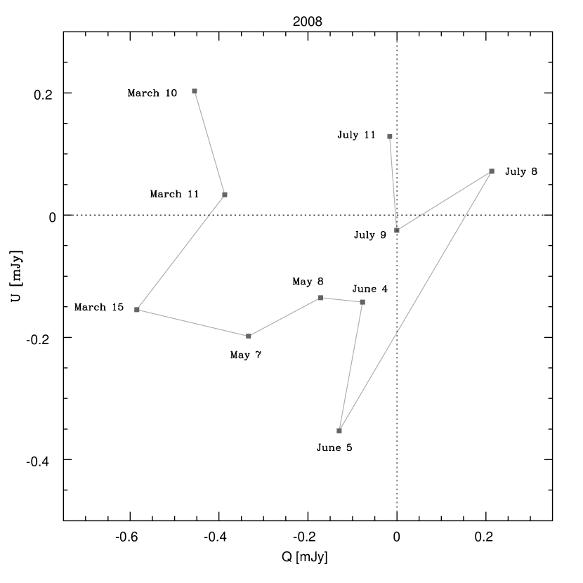
Figure 3: Stokes plane showing the rotation of position angle (EVPA) of the polarization during the flare of 2008 June.

In Cycle I a gradual rotation of the EVPA of 78° (2008 March 10) to 315°(2008 July 9) is observed. This corresponds to a total rotation of $\sim$237°  in a period of 121 days (giving an average rate of rotation of $\sim$ 2°  per day). Figure 3 shows this rotation in the Stokes plane. For more clarity only the more representative points are shown.

In Cycles II to VI, our data show that EVPA have the preferential value mentioned above with mean variations rate $\sim$1.2°per day. In cycle IV, the EVPA reach a maximum value of 114°  while the polarization degree is at its minimum value of 2.4%. And the other way around, when the EVPA shows its minimum value of 6°, the polarization degree shows its maximum value of 16.9%.

3 POLARIMETRIC ANALYSIS

From our observations we have found that W Comae shows, in general, a random polarimetric behavior. This has been explained as due to the presence of one or more variable polarization components overlaid on a stable one. To identify the presence of a stable polarized component, we have used the method suggested by Jones et al. (1985). In this work, the authors proposed that if the observed average values ($\cal h$ $Q$ $\cal i$, $\cal h$ $U$ $\cal i$) in the absolute Stokes parameters plane $Q$-$U$ deviate significantly from the origin, then a stable polarization component is present. From our data, the derived average values of the absolute Stokes parameters are $\langle Q\rangle$ = -0.22$\pm$0.02 mJy and $\langle U\rangle$= 0.21$\pm$0.03 mJy. These average values correspond to a stable component with constant polarization degree $P_{c}=10.7\%\pm 0.8\%$ and polarization angle $\Theta_{c}=$65°$\pm$2$\arcdeg$. The constant polarization degree has a dispersion $\sigma_{P_{c}}=$ 6.4%.

To estimate the polarization variable component parameters, we looked for a possible linear relation between $Q$ versus $I$ and $U$ versus $I$ for the six relevant cycles (see, Hagen-Thorn et al., 2008). For Cycle IV no linear correlation between these parameters was found; rather, they appear to be randomly related. In contrast, for Cycles I, II, III, V, and VI, our data show a linear tendency between these parameters. We made a least square fit to the data in order to find the slopes and the linear correlation coefficients $r_{QI}$ and $r_{UI}$. Figure 4 shows this linear correlations between Stokes parameters for cycles I and VI. The correlation coefficients for these parameters are given in Table 4 where Columns 2 to 7 give the parameters $q_{var}$, $r_{QI}$, $u_{var}$, $r_{UI}$, $p_{\rm var}$ and $\theta_{\rm var}$, respectively. The maximum polarization degree found for the variable component is $p_{\rm var}^{\rm max}\,=\,(40.1\pm 5.1$)%, with a polarization angle $\theta_{\rm var}\,=\,116\arcdeg\pm 7\arcdeg$, corresponding to Cycle I.

3.1 The two-component Model

From the above results we infer the presence of a stable component that we assume associated with the relativistic jet, and also a variable component that can be related to the propagation of a shock. Therefore, the observed polarization would be the result of the overlap of these two optically thin synchrotron components.

Assuming that there are two polarimetic components in W Comae, we have used equations (1) and (2) given in Holmes et al. (1984) and derive the following equations for the parameters associated to the polarized variable component:

$$p^{2}_{\rm var}=\frac{p_{\rm cons}^{2}+p^{2}(1+I_{v/c})^{2}-2pp_{\rm cons}(1+I_{v/c})\cos 2(\theta_{\rm cons}-\theta)}{I_{v/c}^{2}}\;\;,$$ (7)

and

$$\tan 2\theta_{\rm var}=\frac{p(1+I_{v/c})\sin 2\theta-p_{\rm cons}\sin 2\theta_{\rm cons}}{p(1+I_{v/c})\cos 2\theta-p_{\rm cons}\cos 2\theta_{\rm cons}}\;\;.$$ (8)

where $I_{v/c}$ is the flux ratio between the variable to the constant component, and $p$ and $\theta$ are observed polarimetric parameters. This system of equations has five free parameters: $p_{\rm cons}$, $\theta_{\rm cons}$, $p$, $\theta$ and $I_{v/c}$. The system can be resolve if $p_{\rm cons}$ and $\theta_{\rm cons}$ correspond to $P_{\rm cons}$ and $\Theta_{c}$ previously obtained in section 3.

To obtain $I_{v/c}$, we maximize equation ( 7) with respect to $\theta$. From our observacions, $p_{\rm var}$ reaches maximum values when $p\geq p_{\rm cons}$ and $\pi/2\leq 2\,(\theta_{\rm cons}-\theta)\leq\pi$. From the analysis of the Stoke’s parameters in Cycle I, we find maxima values for $p_{var}=$40% (see Table 4). This maximum occurs in 2008 June 7, with $p=$12.7% and $\theta=110\arcdeg$, just a day before the huge gamma-ray flare. With these values we estimate $I_{v/c}=0.57\pm 0.07$. Applying the same procedure in Cycle VI, where the blazar presents a minimum activity state, we find that $I_{v/c}=3.98\pm 0.32$.

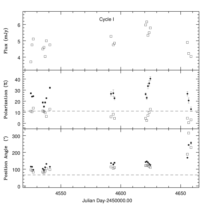
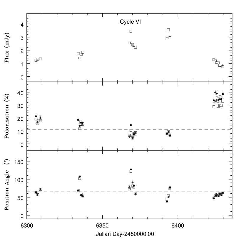
Figure 5: Left and right: empty squares show the observed polarization due to the contribution of the two polarized components, one with constant polarization (dashed line) and another with variable polarization (solid dots). Upper panels show the variations of observed flux. Middle panels, the variations of the the polarized degree. Lower panels, the variations of the EVPA. Left side: In Cycle I the variable polarized component follows the variations of the observed flux, while the observed polarization is weak correlated with it. Right side: In Cycle VI the variations displayed by the the observed polarized degree are followed by the variable polarized component. For more details see Section 3.1.

The values of $p_{\rm var}$ and $\theta_{var}$ are shown in Figure 5, where the observed polarization $p$ is the combination of the two polarization components (stable plus variable). For Cycle I (high activity state) it can be seen that the variable polarization component $p_{\rm var}$ shows a similar variability behavior as the observed flux in the R-band. We previously assumed that this variable polarization component is associated with the propagation of shocks along the jet. In the same figure, we show the results for Cycle VI (low activity state) where the observed polarization $p$ and the variable polarization component $p_{\rm var}$ show a similar variability behavior. It is interesting to note that $\theta_{\rm var}$ follows the observed EVPA variations in both cycles.

4 DISCUSSION

In this work, we have inferred the presence of two components to explain the optical polarization variability. The minimum variability scale of $\sim$3 days was found and it is superimposed on a longer-term flare that lasts $\sim$3 months (these long-term flares appeared separated by $\sim$0.9 yr). The variability timescales found in this work are in agreement with previous studies (Tosti et al., 1998; Massaro et al., 1999).

In 2008 June 8 a strong outburst of very high energy gamma-ray emission above 200 GeV, was detected with VERITAS in W Comae with a significance of 10.3 (Acciari et al., 2009). Data from our monitoring for 2008 June 4-7 show an increase in the $R$-band flux. Unfortunately, due to bad weather we could not obtain data for June 8, when the maximum brightness was observed in the $\gamma$-rays. However, our data show a gradual increase in the value of the EVPA from 78°to 315° (2008 March 10–2008 July 9) and a large rotation of $\sim$237°during cycle I, coinciding with the 2008 flare.

The large rotation of EVPA can be interpreted as due to an asymetric distribution of the magnetic field with respect to the jet axis. Massaro et al. (2001) show that the jet has a spiral structure at 1.6 and 5 GHz. On the other hand, Gabuzda et al. (1994) suggest that the polarization degree and the different values of the EVPA from their VLBI images can be due to shocks propagating along a curved jet, producing an ordered magnetic field with helical structure. These studies found that the jet of W Comae has a projected position angle of $\sim 110^{\circ}$ at 1.6 GHz and 5 GHz. Therefore, the rotation can be produced by a swing of the jet along the visual line of sight, or a curved trajectory of the dissipation/emission pattern. In agreement with Abdo et al. (2010a), the second possibility may be due to the propagation of a knot emission which follows a helical path in a magnetically-dominated jet or can be due to an entire bending of the jet.

The direct association found between the $\gamma$-ray flare in 2008 and the gradual change in the EVPA suggests that the $\gamma$-ray and optical emission regions are co-spatial. This implies a highly ordered magnetic field in regions where the $\gamma$-rays emission is produced, therefore this strong flare could have been produced by a strong shock. Taking into account the properties mentioned above, we assumed that the strong flare observed in 2008 in optical and in $\gamma$-rays is a combination of two factors. On one hand, if a curved structure of the jet is assumed, the jet direction will be oriented towards the observer with the minimum viewing angle. On the other hand, a strong shock occurred at the same time. We will discuss this hypothesis in the following section.

4.1 Alignment of magnetic field by the Shock

From our results, the moderate anti–correlation found in some flares between the flux and the polarization degree indicates that the magnetic field tends to be aligned with the jet. This result is in agreement with Gabuzda & Cawthorne (1996). However, during the 2008 June major flare, lasting in $\gamma$-rays only three days, the flux correlates with the polarization degree thus suggesting that this event was originated by a transversal shock.

Thus in the observer’s reference frame, the flux of the shocked region is amplified as:

$$F=F_{0}\nu^{-\alpha}\delta^{(3+\alpha)}\;\;,$$ (9)

(see Dermer & Menon, 2009) where $\delta=[\Gamma_{j}(1-\beta\cos\Phi]^{-1}$ is the jet’s Doppler factor, $\beta=(1-\Gamma_{j}^{-2})^{1/2}$ its global velocity in units of speed of light, $\Phi$ is the viewing angle, and $\alpha$ is the spectral index in the optical bands.

The observed degree of polarization $p$ depends on the rest–frame angle between the line of sight and the compression axis $\Psi$, the spectral index $\alpha$, and the shock compression factor $\eta$, which is the ratio of densities of a plasma of relativistic electrons from the shocked to the unshocked region $\eta=\eta_{\rm shock}/\eta_{\rm unshock}$ (Hughes & Miller, 1991):

$$p\approx\frac{\alpha+1}{\alpha+5/3}\frac{(1-\eta^{-2})\sin^{2}\Psi}{2-(1-\eta^{-2})\sin^{2}\Psi}\;\;,$$ (10)

and

$$\Psi=\tan^{-1}\left\{\frac{\sin\Phi}{\Gamma_{j}(\cos\Phi-\sqrt{1-\Gamma_{j}^{-2}})}\right\}\;\;.$$ (11)

Following Acciari et al. (2009), we assumed a bulk Lorentz factor $\Gamma_{j}$ = 20 for W Comae. We also used the value of $\alpha$ = 0.87, given by Tosti et al. (1998).

From equation  (9), we can estimate the Doppler factor as a function of time. The value of $F_{0}$ is determined by $F_{0}=F_{\rm max}\nu^{\alpha}/\delta_{D}^{(3+\alpha)}$, where $F_{\rm max}$ is the maximum observed flux and $\delta_{D}$ is obtained from $\Phi_{0}$, which is calculated from equations (10) and (11) for $p\approx p_{\rm var}^{\rm max}$ this being the maximum value of the polarization degree of the variable component (see Table 4). From Hughes & Miller (1991), for $\Psi=\pi/2$, $\eta$=2.2 which is the minimum compression that produces a degree of linear polarization as high as 45$\%$. This yields to $\Psi_{0}\approx 70\arcdeg$, $\Phi_{0}\approx 2.0\arcdeg$, and $\delta_{D}\approx$26.7 at the maximum polarization of the variable component. Using equations (9), (10), and (11) the physical parameters $\delta,\Phi,\Psi$, and $\eta$ as a function of time were estimated.

In Figure 6, it can be seen that the source shows its maximum brightness (14.25 mag, 2008 June 4 or JD 2454621), and the Doppler factor reaches 26.7, while during the minimum (16.5 mag, 2013 May 13 or JD 2456429) it is 15.6. This corresponds to a maximum variation of $\Delta\delta~{}\sim$11. The viewing angle of the jet $\Phi$, shows a minimum value of 2°.0 and a maximum value of 3°.6, i.e., $\Delta\Phi~{}\sim$1.6. These small variations of the Doppler factor can produce large flux variations while $\Gamma_{j}$ remains constant. In the state of maximum brightness, the viewing angle of the shock $\Psi\sim 70\arcdeg$ undergoes its maximum aberration due to relativistic effects.

A maximum compression of the plasma of $\eta$=1.69 is found, when the polarization degree observed reaches its maximum value of $33\%$ (2013 May 17 or JD 2456429). The minimum compression factor $\eta_{\rm min}$=1.01 is obtained when the polarization degree had a minimum value of 0.6$\%$ (2008 July 9 or JD 245 4656). These, small changes in the compression factor ($\Delta\eta\approx 0.68$) can produce large changes in the polarization

The Doppler factor $\delta_{D}$ is obtained when the $R$-band flux is at its maximum value due to the presence of the shock. Then, the change in the magnetic field intensity due to the shock is estimated assuming that the minimum variability timescale is related to the shock-front thickness. This scale is estimated considering the lifetime of the synchrotron electrons (see, e.g. Hagen-Thorn et al., 2008). The lifetime of the synchrotron electrons for a given frequency $\nu$ in GHz is

$$t_{\rm loss}=4.75\times 10^{2}\left(\frac{1+z}{\delta_{D}\,\nu_{\rm GHz}\,B^{3}}\right)^{1/2}\,\rm days\;.$$ (12)

where $B$ is the magnetic field in Gauss. Since $t_{\rm loss}\approx t_{\rm var}$, for $\delta_{D}$ = 26.7 and $t_{\rm var}=3.3\pm 0.3$ days, equation (12) yields an estimate of the magnetic field intensity, $B=$ 0.12$\pm$0.01 G, and an upper limit for the emission region size of $r_{b}\leq ct_{\rm var}\delta_{D}/(1+z)$ = (2.1$\pm$0.2)$\times 10^{17}$ cm.

Finally, in cycles where no correlation was found between the flux and the polarization degree, the flares could be possibly due to an oblique shock to the jet’s direction, or due to changes in the Doppler factor, related to changes in the viewing angle of the jet. Therefore, three scenarios are proposed to explain the flares observed at different timescales: 1) a shock transverse to the jet axis, ordering the magnetic field parallel to the shock’s plane; 2) an oblique shock with respect to the jet axis produced in an initially disordered magnetic field, produces a final magnetic field with a component almost parallel to the jet axis; 3) variations of the Doppler factor due to changes in the jet axis orientation with respect to the observer’s line of sight.

From the polarimetric analysis, we found that the behavior of the polarized variable flux could be due to the superposition of two optically–thin synchrotron components. One stable with $\theta_{\rm cons}\approx$ 65°, $p_{\rm cons}\approx$11% and the other variable  (see Figure 5). Assuming that the position angle of the radio jet is $\theta_{\rm jet}\approx$110°, we propose that the transversal shocks to the jet axis could be related to the variable component and the oblique shocks to the stable component. Nevertheless, both variable and stable components can be affected by variations of the Doppler factor.

5 CONCLUSIONS

From the photopolarimetric observations of W Comae we found that the source displayed activity during the monitored period. We clearly detect four flares, estimating that the object has a minimum variability scale of 3.3 days and a maximum variability in brightness of 2.27 mag. The maximum degree of linear polarization reached by W Comae during the campaign was 33.8%.

An important observational result is the large rotation of EVPA of $\Delta\theta\sim 237^{\circ}$, associated to the optical flare and coincident with the major $\gamma$-ray flare observed in 2008 June. Subsequently, the polarization angle tends to a preferential orientation of $\sim 65^{\circ}$. The large rotation associated with the flare in $\gamma$-rays suggests that both optical / $\gamma$-ray emissions could be produced in the same jet’s region.

From the analysis of the Stokes parameters, we infer the presence of two optically thin synchrotron components with different polarimetric characteristics: one is a variable component and the other one is stable with a constant degree of polarization of $p_{\rm cons}\approx$11%, and a constant position angle of $\theta_{\rm cons}\approx$ 65°. Assuming that the 2008 June optical flare has originated in a transversal shock propagating down a twisted jet, and that the source is a spherical blob of radius $r_{b}$, moving with a Lorentz’s factor of $\Gamma=20$, from our polarimetric data we estimated a Doppler factor of $\delta_{D}\sim 27$ when the flux was maximum, and a visual angle of the jet $\Phi\sim 2^{\circ}.0$. We also obtained a magnetic field intensity $B\sim$ 0.12 G. Finally, an upper limit for the size of the emission region of $r_{b}\leq 2\times 10^{17}$ cm was estimated.

The variability timescales displayed by W Comae show two main characteristics: (1) There are two components in the light-curve, one contributing to the long-term brightening with timescales going from 2 to 4 months, and the other that contributes to the short timescale variations ($\sim 3$ days). This result is in agreement with Tosti et al. (2002). (2) The Doppler factor changes ($\delta(t)\approx 16-27$) could be due to changes in the viewing angle of the jet, implying flux variations lasting $\sim$0.9 yr.

Based on the the anticorrelation found between the polarization percentage and the flux, we propose that the observed long-term flux behavior can be explained with a spiral jet and a transversal shock-wave models. This anticorrelation depends on the Doppler factor time-variations $\delta(t)$ for a range of values of the viewing angle $\theta(t)$.

From our observations, we found that the EPVA in the optical has a value $\sim$ 110°  in 2008 June 7, a day before the gamma-ray flare. This value is identical to the projected angle of the radio jet found by Gabuzda et al. (1994) and Massaro et al. (2001). Later, after the strong gamma-ray flare finished, the EVPA increases its value up to 315°  in 2008 July 9, and two days after it goes down to 229 deg. During the following cycles the EVPA shows a preferential value of 65°. In a future work, it would be useful to measure the direction of EVPA rotations using also radio data. This will allow us to verify whether the behavior of the EVPA in the optical bands is similar to the EVPA variations studied in the radio-bands.

On the other hand, although Zhang et al. (2008) predicts a flare around 2013, from our data collected in 2013 we did not detect any important outburst in W Comae. Rather, we report a continuos brightness decrease detected since the beginning of 2008, reaching a minimum value in 2013 May. But, this could also be considered as a prelude to a major flare or a flare that could start at the end of 2013.

Figure 1: Photopolarimetric light curves of W Comae from 2008 February 28 to 2013 May 17 : (from top to bottom) $R$–band flux, F(mJy); magnitude, $R$ (mag); percentage of linear polarization in the $R$–band, $p(\%)$; and orientation of the EVPA, $\theta$(^∘). Vertical dashed lines separate the monitoring period into Cycles I to VI. Associated errors are presented in Table 1. $R$–band magnitudes and fluxes have been corrected for the host galaxy contribution (see text for explanation). The $R$-band light curve (top panel) shows a slow decreasing of the mean level flux (dashed line) with a fall of $\sim$3 mJy in 5.2 yr.

Figure 2: Correlations between photopolarimetric observations of W Comae for all data. Top panel: correlation between the $R$–band flux and the polarization degree. Bottom panel: correlation between the $R$–band flux and EVPA. The dotted line at the bottom panel shows the preferred EVPA of 65°.

Figure 4: Left: linear correlation between the Stokes parameter $Q$ vs $I$ (top panel), and $U$ vs $I$ (bottom panel) for Cycle I. The correlation coefficients for this cycle are $r_{QI}$=0.80 and $r_{UI}$=0.96, and the slopes $m_{QI}=-0.24\pm 0.07$ and $m_{UI}=-0.32\pm 0.04$, respectively. Right: linear correlation between the Stokes parameter $Q$ vs $I$ (top panel), and $U$ vs $I$ (bottom panel) for Cycle VI. The correlation coefficients for this cycle are $r_{QI}$=0.51 and $r_{UI}$=0.89, and the slopes $m_{QI}=0.10\pm 0.07$ and $m_{UI}=0.33\pm 0.07$, respectively.

Figure 6: Temporal variability of some physical parameters related to the relativistic jet of W Comae: (from top to bottom) Doppler factor, $\delta(t)$; viewing angle of the jet, $\Phi(t)$; rest-frame viewing angle of the shock, $\Psi(t)$; compression factor of the shocked to the unshocked plasma, $\eta(t)$. These parameters were estimated using the maximum flux value observed during Cycle I. Finally, the lower panel shows the degree of linear polarization, $p$[%], in the $R$-band.

Table 1: POLARIZATION AND PHOTOMETRY IN THE $R$-BAND FOR W Comae

Cycle	Date	JD	$p$	$\epsilon_{p}$	$\theta$	$\epsilon_{\theta}$	$R$	$\epsilon_{R}$	$\rm Flux$	$\epsilon_{\rm Flux}$
		2,450,000.00+	($\%$)	($\%$)	($\arcdeg$)	($\arcdeg$)	(mag)	(mag)	(mJy)	(mJy)
I	2008 Feb 28	4524.9351	11.0	0.3	96	01	14.80	0.04	3.71	0.07
	2008 Feb 29	4525.9038	10.4	0.2	93	01	14.53	0.04	4.75	0.08
	2008 Mar 01	4526.9429	13.7	0.2	82	01	14.45	0.04	5.11	0.09
	2008 Mar 09	4534.8984	11.1	0.4	83	01	14.59	0.04	4.50	0.08
	2008 Mar 10	4535.8706	10.8	0.3	78	01	14.57	0.04	4.60	0.08
	2008 Mar 11	4536.8555	9.6	0.4	88	01	14.70	0.04	4.04	0.07
	2008 Mar 12	4537.9004	6.3	0.3	103	02	14.47	0.04	5.00	0.08
	2008 Mar 15	4540.8467	12.8	0.3	97	01	14.53	0.04	4.75	0.08
	2008 May 05	4591.8618	5.9	0.9	113	03	14.42	0.04	5.27	0.09
	2008 May 07	4593.7847	8.2	1.5	105	04	14.53	0.05	4.75	0.09

Note. — The table is available in its entirety in a machine-readable form in the on-line journal. A portion is shown here for guidance regarding its form and content.

Table 2: VARIABILITY PARAMETERS FOR W Comae

Cycle	Parameter	Average	Max	Min	$\Delta_{max}$	$Y(\%)$	$\mu(\%)$	$\cal F$	$\chi^{2}$
(1)	(2)	(3)	(4)	(5)	(6)	(7)	(8)	(9)	(10)
All	R(mag)	15.06 $\pm$ 00.48	16.52	14.25	2.27	-	-	-	-
	F(mJy)	3.17 $\pm$ 01.26	6.16	0.76	5.40	170.1	39.6	0.78	62705.7
	P(%)	12.52 $\pm$ 06.35	33.82	0.59	33.23	264.6	50.7	0.97	4404.1
	$\theta(\arcdeg)$	72.49 $\pm$ 33.40	314.59	5.54	309.05	425.1	46.1	0.97	13456.4
I	R(mag)	14.50 $\pm$ 00.15	14.80	14.25	0.55	-	-	-	-
	F(mJy)	4.91 $\pm$ 00.66	6.16	3.71	2.45	49.8	13.5	0.25	1119.3
	P(%)	7.86 $\pm$ 03.85	13.70	0.59	13.11	165.7	48.9	0.92	979.7
	$\theta(\arcdeg)$	124.86 $\pm$ 58.80	314.59	77.99	236.60	188.6	47.1	0.60	1858.6
II	R(mag)	14.50 $\pm$ 00.07	14.67	14.36	0.31	-	-	-	-
	F(mJy)	4.90 $\pm$ 00.31	5.55	4.18	1.38	27.9	6.4	0.14	212.3
	P(%)	9.29 $\pm$ 03.32	19.91	5.20	14.71	157.6	35.7	0.59	291.2
	$\theta(\arcdeg)$	74.90 $\pm$ 13.33	116.57	55.02	61.55	80.2	17.8	0.36	211.4
III	R(mag)	14.97 $\pm$ 00.18	15.30	14.72	0.58	-	-	-	-
	F(mJy)	3.21 $\pm$ 00.52	4.00	2.35	1.65	51.4	16.3	0.26	1262.7
	P(%)	15.75 $\pm$ 02.37	18.71	10.93	7.78	48.5	15.0	0.26	205.0
	$\theta(\arcdeg)$	61.16 $\pm$ 07.98	77.96	49.76	28.20	45.8	13.1	0.22	431.3
IV	R(mag)	15.32 $\pm$ 00.20	15.56	14.76	0.80	-	-	-	-
	F(mJy)	2.34 $\pm$ 00.48	3.83	1.83	2.00	85.2	20.5	0.35	1885.4
	P(%)	8.65 $\pm$ 04.11	16.93	2.41	14.52	165.3	47.5	0.75	377.0
	$\theta(\arcdeg)$	53.21 $\pm$ 22.47	113.54	5.54	108.00	200.9	42.2	0.91	1970.1
V	R(mag)	15.08 $\pm$ 00.29	15.68	14.53	1.15	-	-	-	-
	F(mJy)	2.96 $\pm$ 00.73	4.75	1.65	3.09	104.6	24.6	0.48	6645.1
	P(%)	14.31 $\pm$ 04.05	20.75	2.89	17.86	123.3	28.3	0.76	312.8
	$\theta(\arcdeg)$	67.91 $\pm$ 10.66	88.82	42.14	46.68	68.0	15.7	0.36	472.1
VI	R(mag)	15.68 $\pm$ 00.51	16.52	14.84	1.68	-	-	-	-
	F(mJy)	1.82 $\pm$ 00.85	3.55	0.76	2.80	153.7	46.7	0.65	7055.9
	P(%)	17.86 $\pm$ 10.05	33.82	5.32	28.50	158.9	56.3	0.73	1136.3
	$\theta(\arcdeg)$	66.22 $\pm$ 17.77	121.93	44.43	77.50	116.9	26.8	0.47	2393.4

Note. — There are no statistics $Y,\mu,\cal F$ and $\chi^{2}$ for the magnitude due to its logarithmic character.

Table 3: STATISTICAL ANALYSIS OF POLARIZATION AND FLUX CORRELATION

Cycle	Relation	$r$	t-student	Confidence
	parameters			level
(1)	(2)	(3)	(4)	(5)
All	F – p	-0.44 +/-0.02	5.72	no
	F – $\theta$	0.47 +/-0.01	6.25	no
	p – $\theta$	-0.34 +/-0.02	4.17	no
I	F – p	0.93 +/-0.11	5.04	yes
	F – $\theta$	-0.90 +/-0.11	4.15	yes
	p – $\theta$	-0.92 +/-0.15	4.60	yes
II	F – p	-0.88 +/-0.24	4.60	yes
	F – $\theta$	-0.71 +/-0.24	2.47	no
	p – $\theta$	0.53 +/-0.27	1.54	no
III	F – p	-0.82 +/-0.09	4.24	yes
	F – $\theta$	0.81 +/-0.08	4.10	yes
	p – $\theta$	-0.68 +/-0.04	2.81	no
IV	F – p	-0.75 +/-0.07	3.18	no
	F – $\theta$	-0.53 +/-0.16	1.75	no
	p – $\theta$	0.25 +/-0.14	0.75	no
V	F – p	0.16 +/-0.08	0.98	no
	F – $\theta$	-0.39 +/-0.08	2.63	no
	p – $\theta$	-0.22 +/-0.13	1.37	no
VI	F – p	-0.89 +/-0.04	7.68	yes
	F – $\theta$	0.41 +/-0.05	1.81	no
	p – $\theta$	-0.61 +/-0.05	3.07	no

Note. — Pearson’s correlation coefficient, $r$, between the observed parameters: Flux (F); polarization degree (p); and polarization angle ($\theta$). In order to verify the validity of the correlation to $99\%$, we applied a t-student test.

Table 4: STOKES PARAMETERS FOR THE VARIABLE COMPONENT OF W Comae

Cycle	$q_{var}$	$r_{QI}$	$u_{var}$	$r_{UI}$	$p_{var}$ ($\%$)	$\theta_{var}$ ($\arcdeg$)
(1)	(2)	(3)	(4)	(5)	(6)	(7)
I	-0.24 $\pm$ 0.07	0.80	-0.32 $\pm$ 0.04	0.96	40.1 $\pm$ 5.1	116 $\pm$ 07
II	0.13 $\pm$ 0.09	0.48	0.17 $\pm$ 0.08	0.59	21.5 $\pm$ 8.3	26 $\pm$ 20
III	-0.20 $\pm$ 0.04	0.92	-0.20 $\pm$ 0.06	0.82	28.4 $\pm$ 5.2	112 $\pm$ 09
V	-0.13 $\pm$ 0.04	0.62	0.18 $\pm$ 0.05	0.73	21.5 $\pm$ 4.6	63 $\pm$ 10
VI	0.10 $\pm$ 0.07	0.51	0.33 $\pm$ 0.07	0.89	34.1 $\pm$ 6.7	37 $\pm$ 10

Note. — No statistics for Cycle IV is presented because no significant correlation between Q-I or U-I relations was found. Column (6) presents the maximum values of $p_{\rm var}$ found in each cycle. Column (7) presents the values of $\theta_{\rm var}$ corresponding to the $p_{\rm var}$ maximum given in column (6). See Section 3.

References

- Abdo et al. (2010a) Abdo, A. A., Ackermann, M., Ajello, M., et al. 2010a, Nature, 463, 919
- Abdo et al. (2010b) Abdo, A. A., Ackermann, M., Agudo, I., et al. 2010b, ApJ, 716, 30
- Acciari et al. (2008) Acciari, V. A., Aliu, E., Beilicke, M., et al. 2008, ApJ, 684, L73
- Acciari et al. (2009) Acciari, V. A., Aliu, E., Aune, T., et al. 2009, ApJ, 707, 612
- Agudo et al. (2013) Agudo, I., Marscher, A., Jorstad, S. G., & Gómez, J. L. 2013, in Highlights of Spanish Astrophysics VII, 152–157
- Agudo et al. (2010) Agudo, I., Thum, C., Wiesemeyer, H., & Krichbaum, T. P. 2010, ApJS, 189, 1
- Angel & Stockman (1980) Angel, J. R. P., & Stockman, H. S. 1980, ARA&A, 18, 321
- Babadzhanyants & Belokon’ (2002) Babadzhanyants, M. K., & Belokon’, E. T. 2002, Astronomy Reports, 46, 609
- Belokon et al. (2000) Belokon, E. T., Babadzhanyants, M. K., & Pollock, J. T. 2000, A&A, 356, L21
- Blandford & Rees (1978) Blandford, R. D., & Rees, M. J. 1978, in BL Lac Objects, ed. A. M. Wolfe, 328–341
- Böttcher et al. (2002) Böttcher, M., Mukherjee, R., & Reimer, A. 2002, ApJ, 581, 143
- Browne (1971) Browne, I. W. A. 1971, Nature, 231, 515
- Burbidge et al. (1974) Burbidge, G. R., Jones, T. W., & Odell, S. L. 1974, ApJ, 193, 43
- Costamante (2012) Costamante, L. 2012, Mem. Soc. Astron. Italiana, 83, 138
- Dermer & Menon (2009) Dermer, C. D., & Menon, G. 2009, High Energy Radiation from Black Holes: Gamma Rays, Cosmic Rays, and Neutrinos, ed. P. U. Pres, 62
- Fiorucci & Tosti (1996) Fiorucci, M., & Tosti, G. 1996, A&AS, 116, 403
- Fossati et al. (1997) Fossati, G., Celotti, A., Ghisellini, G., & Maraschi, L. 1997, MNRAS, 289, 136
- Gabuzda & Cawthorne (1996) Gabuzda, D. C., & Cawthorne, T. V. 1996, MNRAS, 283, 759
- Gabuzda et al. (1992) Gabuzda, D. C., Cawthorne, T. V., Roberts, D. H., & Wardle, J. F. C. 1992, ApJ, 388, 40
- Gabuzda et al. (1994) Gabuzda, D. C., Mullan, C. M., Cawthorne, T. V., Wardle, J. F. C., & Roberts, D. H. 1994, ApJ, 435, 140
- Hagen-Thorn et al. (2008) Hagen-Thorn, V. A., Larionov, V. M., Jorstad, S. G., et al. 2008, ApJ, 672, 40
- Hartman et al. (1999) Hartman, R. C., Bertsch, D. L., Bloom, S. D., et al. 1999, ApJS, 123, 79
- Heidt & Wagner (1996) Heidt, J., & Wagner, S. J. 1996, A&A, 305, 42
- Holmes et al. (1984) Holmes, P. A., Brand, P. W. J. L., Impey, C. D., et al. 1984, MNRAS, 211, 497
- Hovatta et al. (2009) Hovatta, T., Valtaoja, E., Tornikoski, M., & Lähteenmäki, A. 2009, A&A, 494, 527
- Hughes & Miller (1991) Hughes, P. A., & Miller, L. 1991, Introduction: synchrotron and inverse-Compton radiation, ed. P. A. Hughes, 1
- Jones et al. (1985) Jones, T. W., Rudnick, L., Aller, H. D., et al. 1985, ApJ, 290, 627
- Jorstad et al. (2005) Jorstad, S. G., Marscher, A. P., Lister, M. L., et al. 2005, AJ, 130, 1418
- Liu et al. (1995) Liu, F. K., Xie, G. Z., & Bai, J. M. 1995, A&A, 295, 1
- Marscher et al. (2010) Marscher, A. P., Jorstad, S. G., Larionov, V. M., et al. 2010, ApJ, 710, L126
- Massaro et al. (2001) Massaro, E., Mantovani, F., Fanti, R., et al. 2001, A&A, 374, 435
- Massaro et al. (1999) Massaro, E., Maesano, M., Montagni, F., et al. 1999, A&A, 342, L49
- Nieppola et al. (2006) Nieppola, E., Tornikoski, M., & Valtaoja, E. 2006, A&A, 445, 441
- Nilsson et al. (2007) Nilsson, K., Pasanen, M., Takalo, L. O., et al. 2007, A&A, 475, 199
- Nilsson et al. (2003) Nilsson, K., Pursimo, T., Heidt, J., et al. 2003, A&A, 400, 95
- Padovani & Giommi (1995) Padovani, P., & Giommi, P. 1995, ApJ, 444, 567
- Sasada et al. (2011) Sasada, M., Uemura, M., Fukazawa, Y., et al. 2011, PASJ, 63, 489
- Schmidt et al. (1992) Schmidt, G. D., Elston, R., & Lupie, O. L. 1992, AJ, 104, 1563
- Sorcia et al. (2013) Sorcia, M., Benítez, E., Hiriart, D., et al. 2013, ApJS, 206, 11
- Tagliaferri et al. (2000) Tagliaferri, G., Ghisellini, G., Giommi, P., et al. 2000, A&A, 354, 431
- Tosti et al. (1998) Tosti, G., Fiorucci, M., Luciani, M., et al. 1998, A&AS, 130, 109
- Tosti et al. (2002) Tosti, G., Massaro, E., Nesci, R., et al. 2002, A&A, 395, 11
- Zhang et al. (2008) Zhang, X., Zheng, Y. G., Zhang, L., et al. 2008, PASJ, 60, 145