Approximation of mild solutions of the linear and nonlinear elliptic equations

Abstract

In this paper, we investigate the Cauchy problem for both linear and semi-linear elliptic equations. In general, the equations have the form

$$\frac{\partial^{2}}{\partial t^{2}}u\left(t\right)=\mathcal{A}u\left(t\right)+f\left(t,u\left(t\right)\right),\quad t\in\left[0,T\right],$$

where $\mathcal{A}$ is a positive-definite, self-adjoint operator with compact inverse. As we know, these problems are well-known to be ill-posed. On account of the orthonormal eigenbasis and the corresponding eigenvalues related to the operator, the method of separation of variables is used to show the solution in series representation. Thereby, we propose a modified method and show error estimations in many accepted cases. For illustration, two numerical examples, a modified Helmholtz equation and an elliptic sine-Gordon equation, are constructed to demonstrate the feasibility and efficiency of the proposed method.

Keywords and phrases: Elliptic equation; Cauchy problem; Ill-posed problem; Regularization method; Contraction principle.

Mathematics subject Classification 2000: 35K05, 35K99, 47J06, 47H10x.

1 Introduction

The Cauchy problem of elliptic equation plays an important role in inverse problems. For example, in optoelectronics, the determination of a radiation field surrounding a source of radiation (e.g., a light emitting diode) is a frequently occurring problem. As a rule, experimental determination of the whole radiation field is not possible. Practically, we are able to measure the electromagnetic field only on some subset of physical space (e.g., on some surfaces). So, the problem arises how to reconstruct the radiation field from such experimental data (see, for instance, [27]). In the paper of Reginska [27], the authors considered a physical problem which is connected with the notion of light beams. Some applications of this model can be established in more detail in [27]. Another application in inverse obstacle problems (cf. [4]), which are investigated in connection with inclusion detection by electrical impedance tomography when only one pair of boundary current and voltage is used for probing the examined body [24].

Let $\mathcal{H}$ be a real Hilbert space, and let $\mathcal{A}:\mathcal{D}\left(\mathcal{A}\right)\subset\mathcal{H}\to\mathcal{H}$ be a positive-definite, self-adjoint operator with compact inverse on $\mathcal{H}$. In this paper, we consider the problem of finding a function $u:\left[0,T\right]\to\mathcal{H}$ satisfying

$$\frac{\partial^{2}}{\partial t^{2}}u\left(t\right)=\mathcal{A}u\left(t\right)+f\left(t,u\left(t\right)\right),\quad t\in\left[0,T\right],$$ (1)

associated with the initial conditions

$$u\left(0\right)=\varphi,\quad\frac{\partial}{\partial t}u\left(0\right)=g,$$ (2)

where $f$ is a mapping from $\left[0,T\right]\times\mathcal{H}\to\mathcal{H}$, $\varphi$ and $g$ are the exact data in $\mathcal{H}$. Physically, the exact data can only be measured, there will be measurement errors, and we thus would have as data some function $\varphi^{\epsilon}$ and $g^{\epsilon}$ in $\mathcal{H}$ for which

$$\left\|\varphi-\varphi^{\epsilon}\right\|\leq\epsilon,\quad\left\|g-g^{\epsilon}\right\|\leq\epsilon,$$ (3)

where the constant $\epsilon>0$ represents a bound on the measurement error, $\left\|.\right\|$ denotes the $\mathcal{H}$ norm.

Since Hadamard[12], it is well known that the Cauchy problem of elliptic equation, for example, Problem (1)-(2), is severely ill-posed: although it has at most one solution, it may have none, and if a solution exists, it does not depend continuously on the data $\varphi,g$ in any reasonable topology. Therefore, regularization is needed to stabilize the problem. In recent years, many special regularization methods for the homogeneous and nonhomogeneous Cauchy problem of elliptic equation have been proposed, such as Backus-Gilbert algorithm [10], the method of wavelet [14], quasi-reversibility method [21], truncation method [30], non-local boundary value method [11] and the references therein.

Although we have many works on the linear homogeneous case of Cauchy problem for elliptic equation, however, regularization theory and numerical simulation for nonlinear elliptic equations are still limited. Especially, the nonlinear cases for elliptic equation appear in many real applications. For example, let us see a simple one infered by giving $\mathcal{A}=\dfrac{-\partial^{2}}{\partial x^{2}}$ and $\mathcal{D}\left(\mathcal{A}\right)=H_{0}^{1}\left(0,\pi\right)\subset\mathcal{H}=L^{2}\left(0,\pi\right)$ in the problem (1)-(2). In particular, it is given by

$$\begin{cases}\frac{\partial^{2}}{\partial t^{2}}u\left(x,t\right)+\frac{\partial^{2}}{\partial x^{2}}u\left(x,t\right)=f\left(x,t,u\left(x,t\right)\right)&,\left(x,t\right)\in\left(0,\pi\right)\times\left(0,1\right),\\ u\left(0,t\right)=u\left(\pi,t\right)=0&,t\in\left(0,1\right),\\ u\left(x,0\right)=\varphi\left(x\right),\quad\frac{\partial}{\partial t}u\left(x,0\right)=g\left(x\right)&,x\in\left(0,\pi\right).\end{cases}$$ (4)

If $f\left(x,t,u\right)=k^{2}u$ in (4), then it is called Helmholtz equation which has many applications related to wave propagation and vibration phenomena. This equation is often used to describe the vibration of a structure, the acoustic cavity problem, the radiated wave and the scattering of a wave. With $f\left(x,t,u\right)=\sin u$ in (4), we obtain the elliptic sine-Gordon equation. From the point of view of the modelling of physical phenomena, the motivation for the study of this equation comes from its applications in several areas of mathematical physics including the theory of Josephson effects, superconductors and spin waves in ferromagnets, see e.g. [19]. With $f\left(x,t,u\right)=u-u^{3}$, we have the Allen-Cahn equation originally formulated in the description of bi-phase separation in fluids.

Switch back to the considered problem, it is more complicated than the ones above. Hence, the purpose of this paper is to introduce a new method of integral equation that is based on a modification of the exact solution formulation. As the regularization parameter tends to zero, the solution of our regularized problem converges monotonically to the solution of the Cauchy problem with the exact data.

Prior to the approach of main results, we would like to introduce the representation of solution in problem (1)-(2) for linear and semi-linear cases. We can see that the operator $\mathcal{A}$, as a consequence, admits an orthonormal eigenbasis $\left\{\phi_{p}\right\}_{p\geq 1}$ in $\mathcal{H}$, associated with the eigenvalues such that

$$0<\lambda_{1}\leq\lambda_{2}\leq...\lim_{p\to\infty}\lambda_{p}=\infty.$$ (5)

Let $u(t)=\sum\limits_{p=1}^{\infty}\left\langle u(t),\phi_{p}\right\rangle\phi_{p}$ be the Fourier series of $u$ in the Hilbert space $H$. For homogeneous problem, i.e, $f=0$ in (1), by a seperable method, we get the homogeneous second order differential equation as follows

$$\frac{d^{2}}{dt^{2}}\left\langle u(t),\phi_{p}\right\rangle-\lambda_{p}\left\langle u(t),\phi_{p}\right\rangle=0,\left\langle u(0),\phi_{p}\right\rangle=\left\langle\varphi,\phi_{p}\right\rangle,\leavevmode\nobreak\ \frac{d}{dt}\left\langle u(0),\phi_{p}\right\rangle=\left\langle g,\phi_{p}\right\rangle,$$

and its solution leads to

$$u(t)=\sum\limits_{p=1}^{\infty}\left[\cosh\left(\sqrt{\lambda_{p}}t\right)\left\langle\varphi,\phi_{p}\right\rangle+\frac{\sinh\left(\sqrt{\lambda_{p}}t\right)}{\sqrt{\lambda_{p}}}\left\langle g,\phi_{p}\right\rangle\right]\phi_{p},$$ (6)

where $\left\langle.,.\right\rangle$ denotes the inner product in $\mathcal{H}$. From F. Browder terminology, as in [Dan Henry, Geometric Theory of Semi-linear Parabolic Equations, Springer-Verlag, Berlin Heildellberg, Berlin, 1982], $u(t)$ in (6) is called the mild solution of (1)-(2) with $f=0$.

For the nonlinear problem $(1)-(2)$, we say that $u\in C([0,T];H)$ is a mild solution if $u$ satisfies the integral equation

$$u(t)=\sum\limits_{p=1}^{\infty}\left[\cosh\left(\sqrt{\lambda_{p}}t\right)\varphi_{p}+\frac{\sinh\left(\sqrt{\lambda_{p}}t\right)}{\sqrt{\lambda_{p}}}g_{p}+\int\limits_{0}^{t}\frac{\sinh\left(\sqrt{\lambda_{p}}(t-s)\right)}{\sqrt{\lambda_{p}}}f_{p}(u)(s)ds\right]\phi_{p}$$ (7)

where $f_{p}(u)(s)=\left\langle f(s,u(s)),\phi_{p})\right\rangle$. The transformation from problem (1)-(2) into (7) is easily proved by a separation method which is similar above process. From now on, to regularize Problem (1)-(2), we only consider the integral equation (7) and find a regularization method for it. The main idea of integral equation method can be found in a paper [7] on nonlinear backward heat equation.

The paper is organized as follows. In Section 2, we present our regularization method for the linear problem implied by letting $f=0$ in (1). The theoretical results in the Section 2 are inspirable for us to suggest a new regularization method for semi-linear case in Section 3. New convergence estimates are given under some different priori assumptions for the exact solution. Proofs of the results in these sections will be showed in the appendix in the bottom of paper. In Section 4, simple numerical examples aimed to illustrate the main results in Section 3 are analyzed.

2 The linear homogeneous problem

In [21], C.L. Fu and his group applied the quasi-reversibiity (QR ) method to approximate problem (4) in case $f=0$ and $g=0$. The main idea of the original QR method [17] is to approach the ill-posed second order Cauchy problem by a family of well-posed fourth order problems depending on a (small) regularization parameter. In particular, they considered approximate problem

$$\begin{cases}u^{\epsilon}_{tt}\left(x,t\right)+u^{\epsilon}_{xx}\left(x,t\right)-\beta^{2}u^{\epsilon}_{ttxx}\left(x,t\right)=0&,\left(x,t\right)\in\left(0,\pi\right)\times\left(0,1\right),\\ u\left(0,t\right)=u\left(\pi,t\right)=0&,t\in\left(0,1\right),\\ u\left(x,0\right)=\varphi^{\epsilon}\left(x\right),\quad\frac{\partial}{\partial t}u\left(x,0\right)=0&,x\in\left(0,\pi\right).\end{cases}$$ (8)

The solution of (8) is defined by

$$u^{\epsilon}(x,t)=\sum_{p=1}^{\infty}\cosh\left(\frac{pt}{\sqrt{1+\beta^{2}p^{2}}}\right)\left<\varphi^{\epsilon}(x),\sin(px)\right>\sin(px)$$ (9)

and the authors proved that $u^{\epsilon}$ converges to the solution $u$ of homogeneous problem as $\epsilon\to 0$.
Very recently, homogeneous problem has been considered by Hao, Duc and Lesnic [11]. They applied the method of non-local boundary value problems (also called quasi-boundary value method) to regularized the above problem as follows

$$\left\{\begin{gathered}u_{tt}=Au,\hfill\\ u_{t}(0)=0\hfill\\ u(0)+\beta u(aT)=\varphi\hfill\\ \end{gathered}\right.$$ (14)

with $a\geq 1$ being given and $\beta>0$ is the regularization parameter. They proved that the solution to (14) is

$$u^{\alpha}(t)=\sum_{p=1}^{\infty}\frac{\cosh\left(\sqrt{\lambda_{p}}t\right)}{1+\beta\cosh(a\sqrt{\lambda_{p}}t)}\Big{<}\varphi,\phi_{p}\Big{>}\phi_{p}$$ (15)

and $\|u^{\beta}(t)-u(t)\|\to 0$ as $\beta\to 0$ with some assumptions on the exact solution $u$.
Following the work [11], in [30] Tuan, Trong and Quan used a Fourier truncated method to treat the following Cauchy problem of an elliptic equation with nonhomogeneous Dirichlet and Neumann data. From the simple analysis about the exact solution (6), we know that the data error can be arbitrarily amplified by the “kernel” $\cosh\left(\sqrt{\lambda_{p}}t\right)$. That is the reason why the Cauchy problem of elliptic equation is ill-posed. Since the general regularization theory [16] and paper [21], we now give a more general principle of regularization methods for the Cauchy problem of (6). Our idea on regularization method is of constructing a new kernel $Q(t,\lambda_{p},\beta)$ and replacing $\cosh\left(\sqrt{\lambda_{p}}t\right)$ by $Q(t,\lambda_{p},\beta)$ where the new kernel should satisfy

(A) If $\beta$ is fixed, $Q(t,\lambda_{p},\beta)$ is bounded.
(B) If $t,\lambda_{p}$ is fixed, then $\lim_{\beta\to 0}Q(t,\lambda_{p},\beta)=\cosh\left(\sqrt{\lambda_{p}}t\right)$.

Following properties (A) and (B), one can construct other kernels. Furthermore, the idea of properties (A) and (B) can be applied to other ill-posed problems when the solution has the similar form of (6), e.g., the inverse heat conduction problem [26]. In this sense, we say that the properties (A) and (B) are useful and interesting. Now, from above discussion, it is easy to check that the kernels $Q_{1}(t,\lambda_{p},\beta)=\cosh\left(\frac{\sqrt{\lambda_{p}}t}{\sqrt{1+\beta^{2}\lambda_{p}}}\right)$ in [21] and $Q_{2}(t,\lambda_{p},\beta)=\frac{\cosh\left(\sqrt{\lambda_{p}}t\right)}{1+\beta\cosh(a\sqrt{\lambda_{p}}t)}$ in [11] satisfy (A) and (B).

We now have a look at the solution $u$ in (6). To find a regularization solution for $u$, the unstability terms $\cosh\left(\sqrt{\lambda_{p}}t\right)$ and $\sinh\left(\sqrt{\lambda_{p}}t\right)$ in (6) should be replaced by two kernels $Q(t,\lambda_{p},\beta)$ and $R(t,\lambda_{p},\beta)$ respectively. Here the kernel $Q$ satisfies (A), (B) and kernel $R$ satisfies the following conditions

(C) If $\beta$ is fixed, $R(t,\lambda_{p},\beta)$ is bounded.
(D) If $t,\lambda_{p}$ is fixed, then $\lim_{\beta\to 0}R(t,\lambda_{p},\beta)=\sinh\left(\sqrt{\lambda_{p}}t\right)$.

In [30], we choose

$$Q(t,\lambda_{p},\beta)=R(t,\lambda_{p},\beta)=\left\{\begin{gathered}1,\leavevmode\nobreak\ \leavevmode\nobreak\ \text{if}\leavevmode\nobreak\ \leavevmode\nobreak\ \lambda_{p}\leq m_{\beta}^{2},\hfill\\ 0,\leavevmode\nobreak\ \leavevmode\nobreak\ \text{if}\leavevmode\nobreak\ \leavevmode\nobreak\ \lambda_{p}>m_{\beta}^{2},\hfill\\ \end{gathered}\right.$$ (19)

to get a truncation solution (See the fomula (7) in page 2915, [30] ) where $m_{\beta}$ such that $\lim_{\beta\to+\infty m_{\beta}}=+\infty$. It is easy to check that $Q$ and $R$ defined in (19) satisfy $(A),(B)$ and $(C),(D)$ respectively.

In this section, we consider the homogeneous problem of (1) (also given in [30] ) by other choices for kernels. From the formula of $\cosh\left(\sqrt{\lambda_{p}}t\right)$ and $\sinh\left(\sqrt{\lambda_{p}}t\right)$, we realize that the term $e^{\sqrt{\lambda_{p}}t}$ is unstability cause while the term $e^{-\sqrt{\lambda_{p}}t}$ is stable under the boundedness of the unity. Hence, by a simple and natural way, we replace $\cosh\left(\sqrt{\lambda_{p}}t\right)$ and $\sinh\left(\sqrt{\lambda_{p}}t\right)$ by two new kernels

$$Q_{3}(t,\lambda_{p},\beta)=\dfrac{1}{2\beta+2e^{-\sqrt{\lambda_{p}}t}}+\frac{e^{-\sqrt{\lambda_{p}}t}}{2},$$

and

$$R(t,\lambda_{p},\beta)=\dfrac{1}{2\beta+2e^{-\sqrt{\lambda_{p}}t}}-\frac{e^{-\sqrt{\lambda_{p}}t}}{2},$$

to obtain a regularization solution

$$u^{\epsilon}(t)=\sum\limits_{p=1}^{\infty}\left[Q_{3}(t,\lambda_{p},\beta)\left\langle\varphi,\phi_{p}\right\rangle+\frac{R(t,\lambda_{p},\beta)}{\sqrt{\lambda_{p}}}\left\langle g,\phi_{p}\right\rangle\right]\phi_{p}.$$ (20)

Here $\beta=\beta\left(\epsilon\right)$ is called parameter reguarization and satisfies ${\displaystyle\lim_{\epsilon\to 0}\beta\left(\epsilon\right)=0}$. It is easy to check that $Q_{3}$ and $R$ satisfy $(A),(B)$ and $(C),(D)$ respectively. Moreover, (20) leads to

$$u^{\epsilon}\left(t\right)=\sum_{p\geq 1}\left[\dfrac{1}{2\beta+2e^{-\sqrt{\lambda_{p}}t}}\left(\left\langle\varphi,\phi_{p}\right\rangle+\frac{\left\langle g,\phi_{p}\right\rangle}{\sqrt{\lambda_{p}}}\right)+\frac{e^{-\sqrt{\lambda_{p}}t}}{2}\left(\left\langle\varphi,\phi_{p}\right\rangle-\frac{\left\langle g,\phi_{p}\right\rangle}{\sqrt{\lambda_{p}}}\right)\right]\phi_{p}.$$ (21)

Under the inexact data $\varphi^{\epsilon}$ and $g^{\epsilon}$, the regularized solution becomes

$$v^{\epsilon}\left(t\right)=\sum_{p\geq 1}\left[\dfrac{1}{2\beta+2e^{-\sqrt{\lambda_{p}}t}}\left(\left\langle\varphi^{\epsilon},\phi_{p}\right\rangle+\frac{\left\langle g^{\epsilon},\phi_{p}\right\rangle}{\sqrt{\lambda_{p}}}\right)+\frac{e^{-\sqrt{\lambda_{p}}t}}{2}\left(\left\langle\varphi^{\epsilon},\phi_{p}\right\rangle-\frac{\left\langle g^{\epsilon},\phi_{p}\right\rangle}{\sqrt{\lambda_{p}}}\right)\right]\phi_{p}.$$ (22)

Remark 1.

With this linear case of (1) we denote the solution of (1)-(2) by $u\left(t\right)$, the regularized solution of (1)-(2) by $u^{\epsilon}\left(t\right)$, and the regularized solution of (1)-(3) by $v^{\epsilon}\left(t\right)$.

The main results of this section are in the following theorem.

Theorem 2.

Let $\beta=\epsilon^{m}$ for $m\in\left(0,1\right)$.

(i)

If there is a positive constant $E_{1}$ such that

$$\sqrt{\frac{\left\|u\left(T\right)\right\|^{2}}{2}+\frac{\left\|\dfrac{\partial}{\partial t}u\left(T\right)\right\|^{2}}{2\lambda_{1}}}<E_{1},$$ (23)

then we have

$$\begin{cases}\left\|u\left(t\right)-v^{\epsilon}\left(t\right)\right\|\leq\sqrt{2\left(1+\frac{1}{\lambda_{1}}\right)}\epsilon^{1-m}+E_{1}\epsilon^{m}&,t\in\left[0,\frac{T}{2}\right],\\ \left\|u\left(t\right)-v^{\epsilon}\left(t\right)\right\|\leq\sqrt{2\left(1+\frac{1}{\lambda_{1}}\right)}\epsilon^{1-m}+E_{1}\epsilon^{\frac{m\left(T-t\right)}{t}}&,t\in\left[\frac{T}{2},T\right].\end{cases}$$ (24)

(ii)

If there is a positive constant $E_{2}$ such that

$$\sqrt{\sum_{p\geq 1}e^{2\sqrt{\lambda_{p}}\left(T-t\right)}\left(\sqrt{\lambda_{p}}\left\langle u\left(t\right),\phi_{p}\right\rangle+\left\langle\dfrac{\partial}{\partial t}u\left(t\right),\phi_{p}\right\rangle\right)^{2}}<E_{2},$$ (25)

then we have

$$\begin{cases}\left\|u\left(t\right)-v^{\epsilon}\left(t\right)\right\|\leq\sqrt{2\left(1+\frac{1}{\lambda_{1}}\right)}\epsilon^{1-m}+\frac{\epsilon^{m}}{2\sqrt{\lambda_{1}}}E_{2}&,t\in\left[0,\frac{T}{2}\right],\\ \left\|u\left(t\right)-v^{\epsilon}\left(t\right)\right\|\leq\sqrt{2\left(1+\frac{1}{\lambda_{1}}\right)}\epsilon^{1-m}+\frac{\epsilon^{\frac{m\left(T-t\right)}{t}}}{2\sqrt{\lambda_{1}}}\left[\frac{\lambda_{1}T}{1+\ln\left(\frac{\sqrt{\lambda_{1}}T}{\epsilon^{m}}\right)}\right]^{\frac{2t-T}{t}}E_{2}&,t\in\left[\frac{T}{2},T\right].\end{cases}$$ (26)

(iii)

If there is a positive constant $E_{3}$ such that

$$\sqrt{\sum_{p\geq 1}e^{2\sqrt{\lambda_{p}}t}\left(\left\langle\sqrt{\lambda_{p}}u\left(t\right)+\dfrac{\partial}{\partial t}u\left(t\right),\phi_{p}\right\rangle\right)^{2}}<E_{3},$$ (27)

then we have

$$\left\|u\left(t\right)-v^{\epsilon}\left(t\right)\right\|\leq\sqrt{2\left(1+\frac{1}{\lambda_{1}}\right)}\epsilon^{1-m}+E_{3}\frac{\epsilon^{m}}{2}.$$ (28)

In order to prove this theorem, we have to obtain some auxiliary results given by the lemmas below.

Lemma 3.

Let $0<\beta<1$ and let $u^{\epsilon}\left(t\right),v^{\epsilon}\left(t\right)\in\mathcal{H}$ as introduced in Remark 1. Then, we have the following estimate

$$\left\|u^{\epsilon}\left(t\right)-v^{\epsilon}\left(t\right)\right\|\leq\sqrt{2\left(1+\frac{1}{\lambda_{1}}\right)}\epsilon\beta^{-1}.$$ (29)

Lemma 4.

Let $0<\beta<1$ and let $u\left(t\right),v^{\epsilon}\left(t\right)\in\mathcal{H}$ as introduced in Remark 1. If (23) is satisfied, then we have the following estimate

$$\begin{cases}\left\|u\left(t\right)-v^{\epsilon}\left(t\right)\right\|\leq\beta E_{1}&,t\in\left[0,\frac{T}{2}\right],\\ \left\|u\left(t\right)-v^{\epsilon}\left(t\right)\right\|\leq\beta^{\frac{T-t}{t}}E_{1}&,t\in\left[\frac{T}{2},T\right].\end{cases}$$ (30)

Lemma 5.

Let $0<\beta<1$ and let $u\left(t\right),v^{\epsilon}\left(t\right)\in\mathcal{H}$ as introduced in Remark 1. If (25) is satisfied, then we have

$$\begin{cases}\left\|u\left(t\right)-v^{\epsilon}\left(t\right)\right\|\leq\frac{\beta}{2\sqrt{\lambda_{1}}}E_{2}&,t\in\left[0,\frac{T}{2}\right],\\ \left\|u\left(t\right)-v^{\epsilon}\left(t\right)\right\|\leq\frac{1}{2\sqrt{\lambda_{1}}}\beta^{\frac{T-t}{t}}E_{2}&,t\in\left[\frac{T}{2},T\right].\end{cases}$$ (31)

Lemma 6.

Let $0<\beta<1$ and let $u\left(t\right),v^{\epsilon}\left(t\right)\in\mathcal{H}$ as introduced in Remark 1. If (27) is satisfied, then the following estimate holds

$$\left\|u\left(t\right)-v^{\epsilon}\left(t\right)\right\|\leq\frac{\beta}{2}E_{3}.$$ (32)

Remark 7.

At $t=T$, the error in case (i) is useless while it is useful in case (ii). Moreover, in case (iii), under the strong assumptions of $u$, we get the error of Holder-logarithmic type. In fact, if $\epsilon$ is fixed then the right-hand side of (28) get its maximum value at $m=\dfrac{1}{2}$. Thus, we obtain the error of order $\epsilon^{\frac{1}{2}}$.

On the other hand, the condition in (25) is accepted and natural. Thus, we prove that

$$e^{\sqrt{\lambda_{p}}\left(T-t\right)}\left(\sqrt{\lambda_{p}}\left\langle u\left(t\right),\phi_{p}\right\rangle+\left\langle\frac{\partial}{\partial t}u\left(t\right),\phi_{p}\right\rangle\right)=\sqrt{\lambda_{p}}\left\langle u\left(T\right),\phi_{p}\right\rangle+\left\langle\frac{\partial}{\partial t}u\left(T\right),\phi_{p}\right\rangle.$$ (33)

Then the condition

$$\sum_{p\geq 1}\left(\sqrt{\lambda_{p}}\left\langle u\left(T\right),\phi_{p}\right\rangle+\left\langle\frac{\partial}{\partial t}u\left(T\right),\phi_{p}\right\rangle\right)^{2}<\infty,$$ (34)

is easy to check.

3 The semi-linear problem

As we introduced, many previous papers only regularized problems related to (1) in which $f=0$. This condition makes the applicability of the method very narrow. Until now, the results in nonlinear case are very rare. In this section, we consider the problem (1) where $f:R\times\mathcal{H}\to\mathcal{H}$ is a Lipschitz continuous function, i.e., there exists $K>0$ independent of $w_{1},w_{2}\in\mathcal{H},t\in R$ such that

$$\left\|f\left(t,w_{1}\right)-f\left(t,w_{2}\right)\right\|\leq K\left\|w_{1}-w_{2}\right\|.$$ (35)

Since $0<t<s\leq T$ , we know from (7) that, when $p$ becomes large, the terms

$$\cosh\left(\sqrt{\lambda_{p}}t\right),\sinh\left(\sqrt{\lambda_{p}}t\right),\sinh\left(\sqrt{\lambda_{p}}(t-s)\right),$$

increases rather quickly. Thus, these terms are the unstability causes. Hence, to find a regularization solution, we have to replace these terms by new kernels (called stability terms). These kernels have some common properties $(A),(B),(C),(D)$. In fact, we define a following regularization solution

$$u^{\epsilon}(t)=\sum_{p\geq 1}\left[P(t,\lambda_{p},\beta)\varphi_{p}+\frac{Q(t,\lambda_{p},\beta)}{\sqrt{\lambda_{p}}}g_{p}+\int\limits_{0}^{t}\frac{R(t,s,\lambda_{p},\beta)}{\sqrt{\lambda_{p}}}f_{p}(u^{\epsilon})(s)ds\right]\phi_{p}.$$ (36)

Here, $P(t,\lambda_{p},\beta),\leavevmode\nobreak\ Q(t,\lambda_{p},\beta),\leavevmode\nobreak\ R(t,s,\lambda_{p},\beta)$ are bounded by $C(\beta)$ for any $\lambda_{p}>0$. Moreover, if $t,\leavevmode\nobreak\ \lambda_{p}$ fixed then

$$\lim_{\beta\to 0}P(t,\lambda_{p},\beta)=\cosh\left(\sqrt{\lambda_{p}}t\right),\leavevmode\nobreak\ \lim_{\beta\to 0}Q(t,\lambda_{p},\beta)=\sinh\left(\sqrt{\lambda_{p}}t\right),$$

$$\lim_{\beta\to 0}R(t,s,\lambda_{p},\beta)=\sinh\left(\sqrt{\lambda_{p}}(t-s)\right).$$

By direct computation, we see that the kernels in Theorem 1 is not applied to nonlinear problem. For solving this problem, we find some suitable kernels as follows

$$P(t,\lambda_{p},\beta) = \frac{e^{-\sqrt{\lambda_{p}}\left(T-t\right)}}{2\beta\sqrt{\lambda_{p}}+2e^{-\sqrt{\lambda_{p}}T}}+\frac{e^{-\sqrt{\lambda_{p}}t}}{2},$$

$$Q(t,\lambda_{p},\beta) = \frac{e^{-\sqrt{\lambda_{p}}\left(T-t\right)}}{2\beta\sqrt{\lambda_{p}}+2e^{-\sqrt{\lambda_{p}}T}}-\frac{e^{-\sqrt{\lambda_{p}}t}}{2},$$

$$R(t,s,\lambda_{p},\beta) = \frac{e^{-\sqrt{\lambda_{p}}\left(T+s-t\right)}}{2\beta\sqrt{\lambda_{p}}+2e^{-\sqrt{\lambda_{p}}T}}-\frac{e^{-\sqrt{\lambda_{p}}(t-s)}}{2}.$$

Then, we show error estimates between the solution $u\left(t\right)$ and the regularized solution $v^{\epsilon}\left(t\right)$ in $\mathcal{H}$ norm under some supplementary error estimates and assumptions. Simultaneously, the uniqueness of solution $u^{\epsilon},v^{\epsilon}\in C\left(\left[0,T\right];\mathcal{H}\right)$ is proved by contraction principle.

Generally speaking, we obtain the following theorem.

Theorem 8.

Let ${\displaystyle u\left(t\right)=\sum_{p\geq 1}\left\langle u\left(t\right),\phi_{p}\right\rangle\phi_{p}}$ be the solution as denoted in (7). Suppose there is a positive constant $P$ such that

$$4\sup_{0\leq t\leq T}\sum_{p\geq 1}e^{\sqrt{\lambda_{p}}\left(T-t\right)}\left(\sqrt{\lambda_{p}}\left\langle u\left(t\right),\phi_{p}\right\rangle+\left\langle\frac{\partial}{\partial t}u\left(t\right),\phi_{p}\right\rangle\right)^{2}\leq P.$$ (37)

Then by letting $\beta=\epsilon^{m},m\in\left(0,1\right)$ the problem

$$v^{\epsilon}\left(t\right) = \sum_{p\geq 1}\left[\Phi\left(\beta,\lambda_{p},t\right)\mathcal{M}_{p}\left(\varphi^{\epsilon},g^{\epsilon}\right)+\int_{0}^{t}\Psi\left(\beta,\lambda_{p},s,t\right)\left\langle f\left(s,v^{\epsilon}\left(s\right)\right),\phi_{p}\right\rangle ds\right]\phi_{p}$$ (38)

$$+\sum_{p\geq 1}\left[\frac{e^{-\sqrt{\lambda_{p}}t}}{2}\mathcal{M}_{p}\left(\varphi^{\epsilon},-g^{\epsilon}\right)-\int_{0}^{t}\frac{e^{\sqrt{\lambda_{p}}\left(s-t\right)}}{2\sqrt{\lambda_{p}}}\left\langle f\left(s,v^{\epsilon}\left(s\right)\right),\phi_{p}\right\rangle ds\right]\phi_{p}.$$

has a unique solution $v^{\epsilon}\in C\left(\left[0,T\right];\mathcal{H}\right)$ satisfying

$$\left\|u\left(t\right)-v^{\epsilon}\left(t\right)\right\|\leq Q\epsilon^{\frac{m\left(T-t\right)}{T}}T^{\frac{t}{T}}\left(\ln\left(\frac{T}{\epsilon^{m}}\right)\right)^{\frac{-t}{T}},$$ (39)

where for each $p\geq 1$, $\mathcal{M}_{p}:\mathcal{H}\times\mathcal{H}\to R$ such that for $w_{1},w_{2}\in\mathcal{H}$

$$\mathcal{M}_{p}\left(w_{1},w_{2}\right)=\left\langle w_{1},\phi_{p}\right\rangle+\frac{\left\langle w_{2},\phi_{p}\right\rangle}{\sqrt{\lambda_{p}}},$$ (40)

and

$$\Phi\left(\beta,\lambda_{p},t\right)=\frac{e^{-\sqrt{\lambda_{p}}\left(T-t\right)}}{2\beta\sqrt{\lambda_{p}}+2e^{-\sqrt{\lambda_{p}}T}},\quad\Psi\left(\beta,\lambda_{p},s,t\right)=\frac{e^{-\sqrt{\lambda_{p}}\left(T+s-t\right)}}{2\beta\lambda_{p}+2\sqrt{\lambda_{p}}e^{-\sqrt{\lambda_{p}}T}},$$ (41)

$$Q=\sqrt{\frac{3\lambda_{1}+3}{\lambda_{1}}}e^{\frac{3K^{2}T^{2}t}{2\lambda_{1}}}+e^{\frac{K^{2}T^{2}t}{2\lambda_{1}}}\sqrt{P}.$$ (42)

The following lemmas will lead to proof of the main theorem.

Lemma 9.

Let $\Phi\left(\beta,\lambda_{p},t\right)$ and $\Psi\left(\beta,\lambda_{p},s,t\right)$ be defined in (41), then it follows that

$$\Phi\left(\beta,\lambda_{p},t\right)\leq\frac{1}{2}\left(\frac{\beta}{T}\right)^{\frac{-t}{T}}\left(\ln\left(\frac{T}{\beta}\right)\right)^{\frac{-t}{T}},$$ (43)

$$\Psi\left(\beta,\lambda_{p},s,t\right)\leq\frac{1}{2\sqrt{\lambda_{1}}}\left(\frac{\beta}{T}\right)^{\frac{s-t}{T}}\left(\ln\left(\frac{T}{\beta}\right)\right)^{\frac{s-t}{T}}.$$ (44)

Lemma 10.

The following integral equation

$$v^{\epsilon}\left(t\right) = \sum_{p\geq 1}\left[\Phi\left(\beta,\lambda_{p},t\right)\mathcal{M}_{p}\left(\varphi^{\epsilon},g^{\epsilon}\right)+\int_{0}^{t}\Psi\left(\beta,\lambda_{p},s,t\right)\left\langle f\left(s,v^{\epsilon}\left(s\right)\right),\phi_{p}\right\rangle ds\right]\phi_{p}$$ (45)

$$+\sum_{p\geq 1}\left[\frac{e^{-\sqrt{\lambda_{p}}t}}{2}\mathcal{M}_{p}\left(\varphi^{\epsilon},-g^{\epsilon}\right)-\int_{0}^{t}\frac{e^{\sqrt{\lambda_{p}}\left(s-t\right)}}{2\sqrt{\lambda_{p}}}\left\langle f\left(s,v^{\epsilon}\left(s\right)\right),\phi_{p}\right\rangle ds\right]\phi_{p},$$

has a unique solution $v^{\epsilon}\in C\left(\left[0,T\right];\mathcal{H}\right)$.

Lemma 11.

The problem

$$u^{\epsilon}\left(t\right) = \sum_{p\geq 1}\left[\Phi\left(\beta,\lambda_{p},t\right)\mathcal{M}_{p}\left(\varphi,g\right)+\int_{0}^{t}\Psi\left(\beta,\lambda_{p},s,t\right)\left\langle f\left(s,u^{\epsilon}\left(s\right)\right),\phi_{p}\right\rangle ds\right]\phi_{p}$$ (46)

$$+\sum_{p\geq 1}\left[\frac{e^{-\sqrt{\lambda_{p}}t}}{2}\mathcal{M}_{p}\left(\varphi,-g\right)-\int_{0}^{t}\frac{e^{\sqrt{\lambda_{p}}\left(s-t\right)}}{2\sqrt{\lambda_{p}}}\left\langle f\left(s,u^{\epsilon}\left(s\right)\right),\phi_{p}\right\rangle ds\right]\phi_{p},$$

has a unique solution $u^{\epsilon}\in C\left(\left[0,T\right];\mathcal{H}\right)$ and the error estimate holds

$$\left\|v^{\epsilon}\left(t\right)-u^{\epsilon}\left(t\right)\right\|\leq\sqrt{\frac{3\lambda_{1}+3}{\lambda_{1}}}e^{\frac{3K^{2}T^{2}t}{2\lambda_{1}}}\left(\frac{\beta}{T}\right)^{\frac{-t}{T}}\left(\ln\left(\frac{T}{\beta}\right)\right)^{\frac{-t}{T}}\epsilon.$$ (47)

Lemma 12.

Let $u^{\epsilon}\left(t\right)$ be a function defined in (46), then the following estimate holds

$$\left\|u\left(t\right)-u^{\epsilon}\left(t\right)\right\|\leq e^{\frac{T^{2}K^{2}t}{2\lambda_{1}}}\sqrt{P}\beta\left(\frac{\beta}{T}\right)^{\frac{-t}{T}}\left(\ln\left(\frac{T}{\beta}\right)\right)^{\frac{-t}{T}}.$$ (48)

4 Numerical examples

In this section, we aim to show two numerical examples to validate the accuracy and efficiency of our proposed regularization method for 1-D semi-linear elliptic problems including both linear and nonlinear cases. The examples are involved with the operator $\mathcal{A}=-\dfrac{\partial^{2}}{\partial x^{2}}$ and taken by Hilbert space $\mathcal{H}=L^{2}\left(0,\pi\right)$. Particularly, we give examples of a modified Helmholtz equation and an elliptic sine-Gordon equation to demonstrate how the method works.

The aim of numerical experiments is to observe $\epsilon=10^{-r}$ for $r\in\mathbb{N}$. The couple of $\left(\varphi^{\epsilon},g^{\epsilon}\right)$ plays as measured data with a random noise. More precisely, we take perturbation in couple of exact data $\left(\varphi,g\right)$ to define $\left(\varphi^{\epsilon},g^{\epsilon}\right)$ by the following way.

$$\varphi^{\epsilon}\left(x\right) = \varphi\left(x\right)+\frac{\epsilon\cdot\mbox{rand}}{\sqrt{\pi}},$$

$$g^{\epsilon}\left(x\right) = g\left(x\right)+\frac{\epsilon\cdot\mbox{rand}}{\sqrt{\pi}},$$

where rand is a random number determined in $\left[-1,1\right]$.

Then, the regularized solution (with choosing $m=0.99$) is expected to be closed to the exact solution under a proper discretization. For convergence tests, we would like to introduce two errors: the absolute error at the midpoint $\dfrac{\pi}{2}$ and the relative root mean square (RRMS) error. Also, the 2-D and 3-D graphs are applied and analysed.

To be more coherent, we are going to divide this section into two subsections. The first one is to consider the modified Helmholtz equation and the second one is for the elliptic sine-Gordon equation. As we introduced, they are simply outstanding for many applied problems.

Remark 13.

Generally, the whole process is summarized in the following steps.

Step 1. Given $N,K$ and $M$ to have

$$x_{j}=j\Delta x,\Delta x=\dfrac{1}{K},j=\overline{0,K},$$

$$t_{i}=i\Delta t,\Delta t=\dfrac{1}{M},i=\overline{0,M}.$$

Step 2. Choose $r$, put $v^{\epsilon}\left(x,t_{i}\right)=v_{i}^{\epsilon}\left(x\right),i=\overline{0,M}$ and set $v_{0}^{\epsilon}\left(x\right)=\varphi^{\epsilon}\left(x\right)$. We find

$$V^{\epsilon}\left(x\right)=\begin{bmatrix}v_{0}^{\epsilon}\left(x\right)&v_{1}^{\epsilon}\left(x\right)&...&v_{M}^{\epsilon}\left(x\right)\end{bmatrix}^{T}\in\mathbb{R}^{M+1}.$$

Step 3. For $i=\overline{0,M}$ and $j=\overline{0,K},$ put $v_{i}^{\epsilon}\left(x_{j}\right)=v_{i,j}^{\epsilon}$ and $u\left(x_{j},t_{i}\right)=u_{ji}$, we find the matrices in $\mathbb{R}^{M+1}\times\mathbb{R}^{K+1}$ containing all discrete values of the exact solution $u\left(x,t\right)$ and the regularized solution $v^{\epsilon}\left(x,t\right)$, denoted by $U$ and $V^{\epsilon}$, respectively.

$$U=\begin{bmatrix}u_{0,0}&u_{0,1}&\cdots&u_{0,K}\\ u_{1,0}&u_{1,1}&\cdots&u_{1,K}\\ \vdots&\vdots&\ddots&\vdots\\ u_{M,0}&u_{M,1}&\ldots&u_{M,K}\end{bmatrix},\quad V^{\epsilon}=\begin{bmatrix}v_{0,0}^{\epsilon}&v_{0,1}^{\epsilon}&\cdots&v_{0,K}^{\epsilon}\\ v_{1,0}^{\epsilon}&v_{1,1}^{\epsilon}&\cdots&v_{1,K}^{\epsilon}\\ \vdots&\vdots&\ddots&\vdots\\ v_{M,0}^{\epsilon}&v_{M,1}^{\epsilon}&\ldots&v_{M,K}^{\epsilon}\end{bmatrix}.$$

Step 4. Calculate the errors and present 2-D and 3-D graphs.

$$E\left(t_{i}\right)=\left|u\left(\frac{\pi}{2},t_{i}\right)-v^{\epsilon}\left(\frac{\pi}{2},t_{i}\right)\right|,$$ (49)

$$R\left(t_{i}\right)=\frac{\sqrt{\sum_{0\leq j\leq K}\left|u\left(x_{j},t_{i}\right)-v^{\epsilon}\left(x_{j},t_{i}\right)\right|^{2}}}{\sqrt{\sum_{0\leq j\leq K}\left|u\left(x_{j},t_{i}\right)\right|^{2}}}.$$ (50)

4.1 Example 1

We will consider the following equation.

$$\begin{cases}\frac{\partial^{2}}{\partial t^{2}}u\left(x,t\right)+\frac{\partial^{2}}{\partial x^{2}}u\left(x,t\right)=u\left(x,t\right)&,\left(x,t\right)\in\left(0,\pi\right)\times\left(0,1\right),\\ \frac{\partial}{\partial x}u\left(0,t\right)=u\left(\pi,t\right)=0&,t\in\left(0,1\right),\\ u\left(x,0\right)=\varphi\left(x\right),\quad\frac{\partial}{\partial t}u\left(x,0\right)=0&,x\in\left(0,\pi\right).\end{cases}$$ (51)

Based on $\mathcal{D}\left(\mathcal{A}\right)=\left\{v\in H^{1}\left(0,\pi\right):v\left(\pi\right)=0\right\}$, we get an orthonormal eigenbasis $\phi_{p}\left(x\right)=\sqrt{\dfrac{2}{\pi}}\cos\left(\sqrt{\lambda_{p}}x\right)$ associated with the eigenvalue $\lambda_{p}=\left(p-\dfrac{1}{2}\right)^{2}$ in $L^{2}\left(0,\pi\right)$. In order to ensure the problem (51) has solution with a given Cauchy data $\varphi$, we will construct the exact solution from a function $h$ as follows

$$u\left(x,1\right)=\frac{2}{\pi}\sum_{1\leq p\leq N}\left\langle h\left(\xi\right),\cos\left(\left(p-\frac{1}{2}\right)\xi\right)\right\rangle\cos\left(\left(p-\frac{1}{2}\right)x\right),$$ (52)

where $N$ is a truncation term and $h$ will be chosen later. Then, this problem has a unique solution by applying method of separation of variables.

$$u\left(x,t\right)=\frac{2}{\pi}\sum_{1\leq p\leq N}\frac{\cosh\left(t\sqrt{\left(p-\frac{1}{2}\right)^{2}+1}\right)}{\cosh\left(\sqrt{\left(p-\frac{1}{2}\right)^{2}+1}\right)}\left\langle h\left(\xi\right),\cos\left(\left(p-\frac{1}{2}\right)\xi\right)\right\rangle\cos\left(\left(p-\frac{1}{2}\right)x\right).$$ (53)

Thus, we have

$$\varphi\left(x\right)=\frac{2}{\pi}\sum_{1\leq p\leq N}\frac{\left\langle h\left(\xi\right),\cos\left(\left(p-\frac{1}{2}\right)\xi\right)\right\rangle}{\cosh\left(\sqrt{\left(p-\frac{1}{2}\right)^{2}+1}\right)}\cos\left(\left(p-\frac{1}{2}\right)x\right).$$ (54)

Simultaneously, the regularized solution defined in (38) becomes

$$v^{\epsilon}\left(x,t\right) = \sum_{1\leq p\leq N}\Phi\left(\epsilon,p,t\right)\mathcal{M}_{p}\left(\varphi^{\epsilon},g^{\epsilon}\right)\cos\left(\left(p-\frac{1}{2}\right)x\right)$$

$$+\sum_{1\leq p\leq N}\left(\int_{0}^{t}\int_{0}^{\pi}\Psi\left(\epsilon,p,s,t\right)v^{\epsilon}\left(x,s\right)\cos\left(\left(p-\frac{1}{2}\right)x\right)dxds\right)\cos\left(\left(p-\frac{1}{2}\right)x\right)$$

$$+\frac{1}{2}\sum_{1\leq p\leq N}e^{-\left(p-\frac{1}{2}\right)t}\mathcal{M}_{p}\left(\varphi^{\epsilon},-g^{\epsilon}\right)\cos\left(\left(p-\frac{1}{2}\right)x\right)$$

$$-\sum_{1\leq p\leq N}\left(\frac{2}{\pi\left(2p-1\right)}\int_{0}^{t}\int_{0}^{\pi}e^{\left(p-\frac{1}{2}\right)\left(s-t\right)}v^{\epsilon}\left(x,s\right)\cos\left(\left(p-\frac{1}{2}\right)x\right)dxds\right)\cos\left(\left(p-\frac{1}{2}\right)x\right),$$

where $\mathcal{M}_{p}\left(\varphi^{\epsilon},\pm g^{\epsilon}\right),\Phi\left(\epsilon,p,t\right)$ and $\Psi\left(\epsilon,p,s,t\right)$ are induced by (40)-(41). They are explicitly defined as follows.

$$\mathcal{M}_{p}\left(\varphi^{\epsilon},\pm g^{\epsilon}\right)=\frac{2}{\pi}\int_{0}^{\pi}\left[\varphi^{\epsilon}\left(x\right)\pm\frac{g^{\epsilon}\left(x\right)}{p-\frac{1}{2}}\right]\cos\left(\left(p-\frac{1}{2}\right)x\right)dx,$$ (56)

$$\Phi\left(\epsilon,p,t\right)=\frac{e^{-\left(p-\frac{1}{2}\right)\left(1-t\right)}}{\epsilon^{0.99}\left(2p-1\right)+2e^{-\left(p-\frac{1}{2}\right)}},\quad\Psi\left(\epsilon,p,s,t\right)=\frac{2}{\pi}\frac{e^{-\left(p-\frac{1}{2}\right)\left(1+s-t\right)}}{2\epsilon^{0.99}\left(p-\frac{1}{2}\right)^{2}+\left(2p-1\right)e^{-\left(p-\frac{1}{2}\right)}}.$$ (57)

Now when we divide the time $t_{i}=i\Delta t,\Delta t=\dfrac{1}{M},i=\overline{0,M}$, it turns out that a simple iterative scheme in time is applied to (LABEL:eq:41). Particularly, we will compute $v_{i}^{\epsilon}\left(x\right),i=\overline{1,M}$ from $v_{0}^{\epsilon}\left(x\right)=\varphi^{\epsilon}\left(x\right)$ as follows.

$$v_{i}^{\epsilon}\left(x\right)\equiv v^{\epsilon}\left(x,t_{i}\right)=\sum_{1\leq p\leq N}\left[\mathcal{R}\left(\epsilon,p,t_{i}\right)-\mathcal{W}\left(\epsilon,p,t_{i}\right)\right]\cos\left(\left(p-\frac{1}{2}\right)x\right),$$ (58)

where

$$\mathcal{R}\left(\epsilon,p,t_{i}\right) = \Phi\left(\epsilon,p,t_{i}\right)\mathcal{M}_{p}\left(\varphi^{\epsilon},g^{\epsilon}\right)+\frac{1}{2}e^{-\left(p-\frac{1}{2}\right)t_{i}}\mathcal{M}_{p}\left(\varphi^{\epsilon},-g^{\epsilon}\right)$$ (59)

$$+\sum_{1\leq j\leq i}\int_{t_{j-1}}^{t_{j}}\int_{0}^{\pi}\Psi\left(\epsilon,p,s,t_{i}\right)v_{j-1}^{\epsilon}\left(x\right)\cos\left(\left(p-\frac{1}{2}\right)x\right)dxds,$$

$$\mathcal{W}\left(\epsilon,p,t_{i}\right)=\frac{2}{\pi\left(2p-1\right)}\sum_{1\leq j\leq i}\int_{t_{j-1}}^{t_{j}}\int_{0}^{\pi}e^{\left(p-\frac{1}{2}\right)\left(s-t_{i}\right)}v_{j-1}^{\epsilon}\left(x\right)\cos\left(\left(p-\frac{1}{2}\right)x\right)dxds.$$ (60)

As we know, $h$ plays the role as a test function. From this example, we want to find exactly inner products between the test function and the eigenbasis by choosing simple functions: $x^{2}\left(\pi-x\right)$ and ${\displaystyle\sum_{k=1}^{3}\frac{\cos\left(kx\right)}{k}}$. On the other hand, we note that (59) and (60) can be simplified by directly computing the following integrations.

$$\int_{t_{j-1}}^{t_{j}}\Psi\left(\epsilon,p,s,t_{i}\right)ds=\frac{4}{\pi\left(1-2p\right)}\frac{e^{-\left(p-\frac{1}{2}\right)\left(1+t_{j}-t_{i}\right)}-e^{-\left(p-\frac{1}{2}\right)\left(1+t_{j-1}-t_{i}\right)}}{2\epsilon^{0.99}\left(p-\frac{1}{2}\right)^{2}+\left(2p-1\right)e^{-\left(p-\frac{1}{2}\right)}},$$ (61)

$$\int_{t_{j-1}}^{t_{j}}e^{\left(p-\frac{1}{2}\right)\left(s-t_{i}\right)}ds=\frac{2}{2p-1}\left[e^{\left(p-\frac{1}{2}\right)\left(t_{j}-t_{i}\right)}-e^{\left(p-\frac{1}{2}\right)\left(t_{j-1}-t_{i}\right)}\right].$$ (62)

Test function	$\epsilon$	$E\left(\dfrac{1}{10}\right)$	$E\left(\dfrac{1}{2}\right)$	$E\left(1\right)$
$h\left(x\right)=x^{2}\left(\pi-x\right)$	$10^{-2}$	0.035409705039934	0.116746863516900	0.372168953951916
	$10^{-4}$	0.000431278831272	0.003358920542896	0.023605079336301
	$10^{-6}$	0.000014949076139	0.001913491383348	0.019016995706460
	$10^{-8}$	0.000009993878017	0.001807682028770	0.018567839990525
$h\left(x\right)={\displaystyle\sum_{k=1}^{3}\frac{\cos\left(kx\right)}{k}}$	$10^{-1}$	0.004249941946421	0.074435441315929	0.272260206158619
	$10^{-3}$	0.001582454284463	0.004009212062991	0.014413248824993
	$10^{-5}$	0.000018911820283	0.000313502875558	0.003106592235082
	$10^{-7}$	0.000001421650997	0.000230738814781	0.002877357795009

Table 1: The absolute error at the midpoint defined in (49) with $t=\dfrac{1}{10};\dfrac{1}{2};1$ for both two test functions in Example 1.

Test function	$\epsilon$	$R\left(1\right)$	Test function	$\epsilon$	$R\left(1\right)$
$h\left(x\right)=x^{2}\left(\pi-x\right)$	$10^{-2}$	0.103782899356401	$h\left(x\right)={\displaystyle\sum_{k=1}^{3}\frac{\cos\left(kx\right)}{k}}$	$10^{-1}$	0.497932025244192
	$10^{-4}$	0.005938944110216		$10^{-3}$	0.020910786614042
	$10^{-6}$	0.004681856304455		$10^{-5}$	0.005441953635180
	$10^{-8}$	0.004668575093985		$10^{-7}$	0.005276479332669

Table 2: The RRMS error defined in (50) with $t=1$ for both two test functions in Example 1.

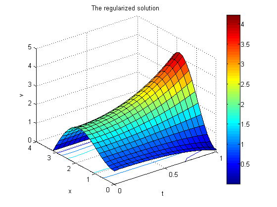
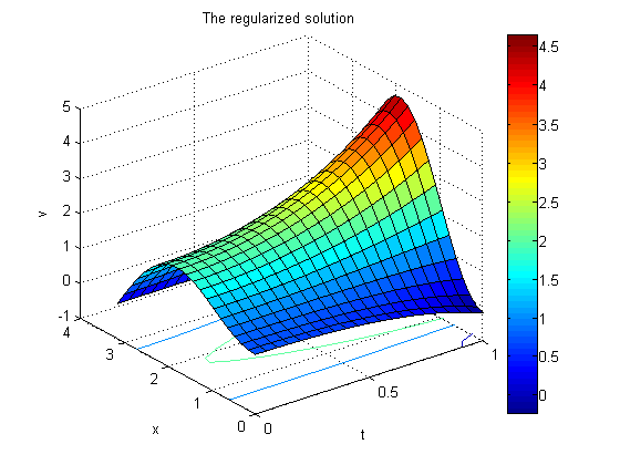
Figure 1: The regularized solution (LABEL:eq:41) of Example 1 for $h\left(x\right)=x^{2}\left(\pi-x\right)$ and $\epsilon=10^{-r}$ with $r=2;4$ in 3-D representation.

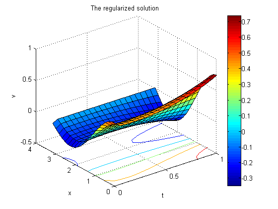
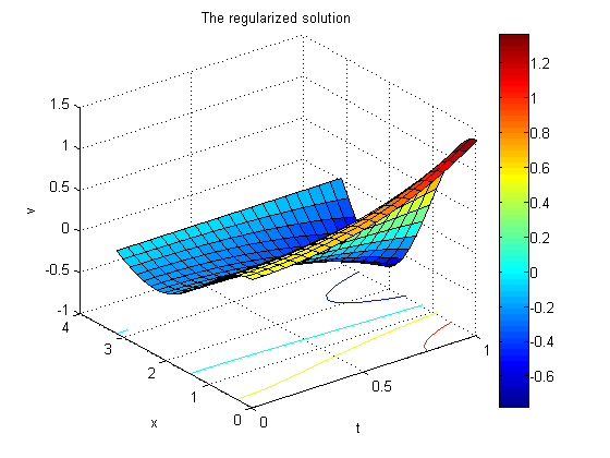
Figure 2: The regularized solution (LABEL:eq:41) of Example 1 for $h\left(x\right)={\displaystyle\sum_{k=1}^{3}\frac{\cos\left(kx\right)}{k}}$ and $\epsilon=10^{-r}$ with $r=1;3$ in 3-D representation.

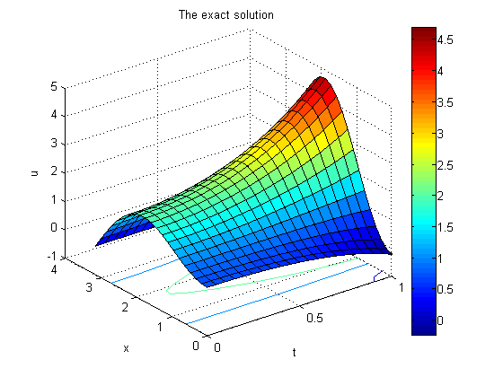
Figure 3: The exact solution (53) for both two test functions in 3-D representation in Example 1.

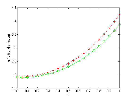
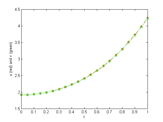
Figure 4: 2-D graphs of the exact solution (red) and regularized solution (green) at $x=\dfrac{\pi}{2}$ for $h\left(x\right)=x^{2}\left(\pi-x\right)$ and $\epsilon=10^{-r}$ with $r=2;4$ in Example 1.

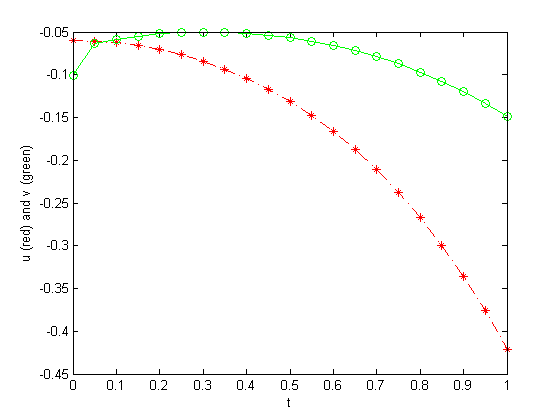
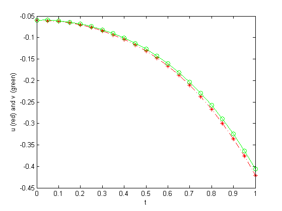
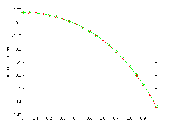
Figure 5: 2-D graphs of the exact solution (red) and regularized solution (green) at $x=\dfrac{\pi}{2}$ for $h\left(x\right)={\displaystyle\sum_{k=1}^{3}\frac{\cos\left(kx\right)}{k}}$ and $\epsilon=10^{-r}$ with $r=1;3;5;7$ in Example 1.

Comments.

In this computations, the square grid size for time and space variables are rawly set by choosing $K=M=20$. The truncation term is simply equal to $N=3$.

Table 1 and Table 2 show the absolute error at the midpoint $\dfrac{\pi}{2}$ and RRMS error defined in (49)-(50) for both two test functions $h$. Particularly, the tables show the errors between the exact solution whose existence is ensured under the test function $h$, recall that in this example we let $h\left(x\right)=x^{2}\left(\pi-x\right)$ and $h\left(x\right)={\displaystyle\sum_{k=1}^{3}\frac{\cos\left(kx\right)}{k}}$, and the regularized solution (LABEL:eq:41) at the fixed time $t=\dfrac{1}{10};\dfrac{1}{2};1$ indicating three basic stage of time, nearly initial-middle-final, are both considered. We observe that the further initial point, the slower convergence speed and the smaller $\epsilon$, the smaller errors.

For the test function $h\left(x\right)=x^{2}\left(\pi-x\right)$, we show the corresponding exact solution in Figure 3 (left) and present. Despite the same 3-D shape, it should be given attention to the color bar of the regularized ones, especially the maximum values attaining on the bar. In addition, Figure 4 present the 2-D graphs of the solutions at $x=\dfrac{\pi}{2}$ for $\epsilon=10^{-2};10^{-4}$. By observation, the regularized solution is close to the exact one when $\epsilon$ gets smaller.

Similarly, for the test function $h\left(x\right)={\displaystyle\sum_{k=1}^{3}\frac{\cos\left(kx\right)}{k}}$ we show in Figure 3 (right) the exact solution and in Figure 2 the regularized solution (LABEL:eq:41) for $\epsilon=10^{-1};10^{-3}$. In Figure 5, we present the 2-D graphs of the solutions at the middle point of space for $\epsilon=10^{-r}$ with $r=1;3;5;7$, respectively.

4.2 Example 2

For this example, we intend to give attention to an elliptic sine-Gordon equation.

$$\begin{cases}\frac{\partial^{2}}{\partial t^{2}}u\left(x,t\right)+\frac{\partial^{2}}{\partial x^{2}}u\left(x,t\right)=\sin\left(u\left(x,t\right)\right)-\sin\left(t\sin x\right)-t\sin x&,\left(x,t\right)\in\left(0,\pi\right)\times\left(0,1\right),\\ u\left(0,t\right)=u\left(\pi,t\right)=0&,t\in\left(0,1\right),\\ u\left(x,0\right)=0,\quad\frac{\partial}{\partial t}u\left(x,0\right)=\sin x&,x\in\left(0,\pi\right).\end{cases}$$ (63)

It is easy to see that for $\mathcal{D}\left(\mathcal{A}\right)=H_{0}^{1}\left(0,\pi\right)$, we have an orthonormal eigenbasis $\phi_{p}\left(x\right)=\sqrt{\dfrac{2}{\pi}}\sin\left(\sqrt{\lambda_{p}}x\right)$ in $L^{2}\left(0,\pi\right)$ and $\lambda_{p}=p^{2}$ is the corresponding eigenvalue. The exact solution is $u\left(x,t\right)=t\sin x$. Similar to (LABEL:eq:41)-(57) in Exampe 1, we establish the regularized solution.

$$v^{\epsilon}\left(x,t\right) = \sum_{1\leq p\leq N}\Phi\left(\epsilon,p,t\right)\mathcal{M}_{p}\left(\varphi^{\epsilon},g^{\epsilon}\right)\sin\left(px\right)$$ (64)

$$+\sum_{1\leq p\leq N}\left(\int_{0}^{t}\int_{0}^{\pi}\Psi\left(\epsilon,p,s,t\right)\sin\left(v^{\epsilon}\left(x,s\right)\right)\sin\left(px\right)dxds\right)\sin\left(px\right)$$

$$+\frac{1}{2}\sum_{1\leq p\leq N}e^{-pt}\mathcal{M}_{p}\left(\varphi^{\epsilon},-g^{\epsilon}\right)\sin\left(px\right)$$

$$+\sum_{1\leq p\leq N}\left(\frac{1}{\pi p}\int_{0}^{t}\int_{0}^{\pi}e^{p\left(s-t\right)}\sin\left(v^{\epsilon}\left(x,s\right)\right)\sin\left(px\right)dxds\right)\sin\left(px\right),$$

where

$$\Phi\left(\epsilon,p,t\right)=\frac{e^{-p\left(1-t\right)}}{2p\epsilon^{0.99}+2e^{-p}},\quad\Psi\left(\epsilon,p,s,t\right)=\frac{1}{\pi}\frac{e^{-p\left(1+s-t\right)}}{p^{2}\epsilon^{0.99}+pe^{-p}},$$ (65)

$$\mathcal{M}_{p}\left(\varphi^{\epsilon},\pm g^{\epsilon}\right)=\frac{2}{\pi}\int_{0}^{\pi}\left[\varphi^{\epsilon}\left(x\right)\pm\frac{g^{\epsilon}\left(x\right)}{p}\right]\sin\left(px\right)dx.$$ (66)

In the same way, we are going to compute $v_{i}^{\epsilon}\left(x\right),i=\overline{1,M}$ from $v_{0}^{\epsilon}\left(x\right)=\varphi^{\epsilon}\left(x\right)$ as (58)-(60). Consequently, the following iterative scheme is in order.

$$v_{i}^{\epsilon}\left(x\right)=\sum_{1\leq p\leq N}\left[\mathcal{R}\left(\epsilon,p,t_{i}\right)-\mathcal{W}\left(\epsilon,p,t_{i}\right)\right]\sin\left(px\right),$$ (67)

where

$$\mathcal{R}\left(\epsilon,p,t_{i}\right) = \Phi\left(\epsilon,p,t_{i}\right)\mathcal{M}_{p}\left(\varphi^{\epsilon},g^{\epsilon}\right)+\frac{1}{2}e^{-pt_{i}}\mathcal{M}_{p}\left(\varphi^{\epsilon},-g^{\epsilon}\right)$$

$$+\sum_{1\leq j\leq i}\int_{t_{j-1}}^{t_{j}}\int_{0}^{\pi}\Psi\left(\epsilon,p,s,t_{i}\right)\left[\sin\left(v_{j-1}^{\epsilon}\left(x\right)\right)-\sin\left(s\sin x\right)-s\sin x\right]\sin\left(px\right)dxds,$$

$$\mathcal{W}\left(\epsilon,p,t_{i}\right) = \frac{1}{\pi p}\sum_{1\leq j\leq i}\int_{t_{j-1}}^{t_{j}}\int_{0}^{\pi}e^{p\left(s-t_{i}\right)}\left[\sin\left(v_{j-1}^{\epsilon}\left(x\right)\right)-\sin\left(s\sin x\right)-s\sin x\right]\sin\left(px\right)dxds,$$ (69)

There is a little bit marked difference in computation between (LABEL:eq:54)-(69) and (59)-(60). In fact, we first split $\mathcal{R}\left(\epsilon,p,t_{i}\right)$ into three appropriate terms, a term $\mathcal{R}_{1}\left(\epsilon,p,t_{i}\right)$ including $\Phi\left(\epsilon,p,t_{i}\right)\mathcal{M}_{p}\left(\varphi^{\epsilon},g^{\epsilon}\right)+\dfrac{1}{2}e^{-pt_{i}}\mathcal{M}_{p}\left(\varphi^{\epsilon},-g^{\epsilon}\right)$, a term $\mathcal{R}_{2}\left(\epsilon,p,t_{i}\right)$ including the nonlinearity $\sin\left(v_{j-1}^{\epsilon}\left(x\right)\right)$ and a term $\mathcal{R}_{3}\left(\epsilon,p,t_{i}\right)$ containing the rest of this sum. In order to compute $\mathcal{R}_{2}\left(\epsilon,p,t_{i}\right)$ and $\mathcal{R}_{3}\left(\epsilon,p,t_{i}\right)$, we apply Gauss-Legendre quadrature method (see in [1]). In particular, we have

$$\int_{t_{j-1}}^{t_{j}}\int_{0}^{\pi}\Psi\left(\epsilon,p,s,t_{i}\right)\sin\left(v_{j-1}^{\epsilon}\left(x\right)\right)\sin\left(px\right)dxds = \frac{1}{\pi}\frac{e^{-p\left(1+t_{j}-t_{i}\right)}-e^{-p\left(1+t_{j-1}-t_{i}\right)}}{p^{2}\epsilon^{0.99}+pe^{-p}}$$ (70)

$$\times\sum_{r=0}^{r_{0}}\gamma_{r}\sin\left(v_{j-1}^{\epsilon}\left(x_{r}\right)\right)\sin\left(px_{r}\right),$$

$$\int_{t_{j-1}}^{t_{j}}\int_{0}^{\pi}\Psi\left(\epsilon,p,s,t_{i}\right)\left[\sin\left(s\sin x\right)+s\sin x\right]\sin\left(px\right)dxds = \sum_{l=0}^{l_{0}}\sum_{r=0}^{r_{0}}\alpha_{l}\gamma_{r}\Psi\left(\epsilon,p,t_{l},t_{i}\right)$$

$$\times\left[\sin\left(t_{l}\sin x_{r}\right)+t_{l}\sin x_{r}\right]\sin\left(px_{r}\right),$$

where $x_{r}$ and $t_{l}$ are abscissae in $\left[0,\pi\right]$ and $\left[t_{j-1},t_{j}\right]$, respectively, and $\alpha_{l},\gamma_{r}$ are associated weights.

We also do the same way in computation of (69). Hence, (67) can be determined.

$\epsilon$	$E\left(\dfrac{1}{10}\right)$	$E\left(\dfrac{1}{2}\right)$	$E\left(1\right)$
$10^{-1}$	0.086458375926430	0.131568588308656	0.221657715167904
$10^{-2}$	0.005697161754899	0.015183097329748	0.056405650468800
$10^{-3}$	0.001067813554645	0.002786056926348	0.014399880506214
$10^{-4}$	0.000104838093802	0.000817994686682	0.008691680983081
$10^{-5}$	0.000035757102538	0.000617861664942	0.007872214352913
$10^{-6}$	0.000019864327276	0.000595051843803	0.007845137692661
$10^{-7}$	0.000017600480787	0.000592557387737	0.007844539150103
$10^{-8}$	0.000017498079817	0.000592334649247	0.007843831738541

$\epsilon$	$R\left(\dfrac{1}{10}\right)$	$R\left(\dfrac{1}{2}\right)$	$R\left(1\right)$
$10^{-1}$	0.799075862748019	0.250473426345937	0.198371536659905
$10^{-2}$	0.041412415178910	0.021481555379548	0.044750235777145
$10^{-3}$	0.008399419222540	0.004819027580652	0.010213755307730
$10^{-4}$	0.000858718982259	0.002391935255341	0.006165668177321
$10^{-5}$	0.000627339975148	0.002359110404713	0.005644668172741
$10^{-6}$	0.000476784804847	0.002314417574336	0.005618874168933
$10^{-7}$	0.000451357224492	0.002306699187820	0.005618134790713
$10^{-8}$	0.000450895426251	0.002306548381426	0.005617676121443

Table 3: The absolute error at the midpoint (top) defined in (49) and RRMS error (bottom) defined in (50) at $t=\dfrac{1}{10};\dfrac{1}{2};1$ in Example 2.

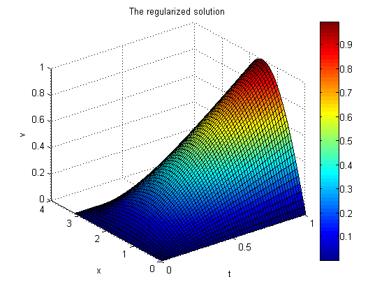
Figure 6: The exact solution $u\left(x,t\right)=t\sin x$ (left) and the regularized solution $v^{\epsilon}\left(x,t\right)$ (right) defined in (64) for $\epsilon=10^{-4}$ in 3-D representation in Example 2.

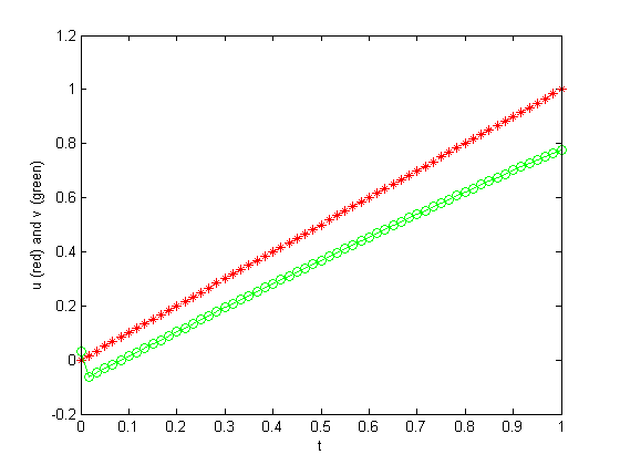
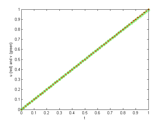
Figure 7: 2-D graphs of the exact solution (red) and regularized solution (green) for $\epsilon=10^{-r}$ with $r=1;4$ in Example 2.

Comments.

In this computations, the finer grid is used $\left(K=M=60\right)$ and the truncation term is still fixed as above. In the same way, we show in Table 3 the errors between the exact solution (with suppose the specific unique solution $u\left(x,t\right)=t\sin x$) and the regularized solution (64). In Figure 6 and Figure 7, 3-D and 2-D graphs of them are shown, respectively. In particular, we show in Figure 7 the 2-D graphs describing how the regularized solution approachs to the exact one when $\epsilon$ becomes smaller and smaller, we illustrate the approach process by simply presenting their graphs for $\epsilon=10^{-1};10^{-4}$. We also show the 3-D representation of the regularized solution (with $\epsilon=10^{-4}$) in Figure 6 (right).

From the numerical results, we can conclude in the same event that the further initial point, the slower convergence speed and the convergence is hold in general. On the other hand, it can be probably observed that the errors reduce slowly when $\epsilon\to 0$ ($\epsilon=10^{-7},10^{-8},...$), and with a finer grid of resolution, we can have a better result in terms of the smaller errors.

5 Conclusion

In this paper, we have studied the modified method to regularize the Cauchy problem for both linear and semi-linear elliptic equations which are severely ill-posed in general. Our approach is to present the solution of the problem in series representation, and then propose the regularized solution to control the strongly increasing coefficients appearing in the series. Under some prior assumptions, we deduce error estimates between the exact solution and regularized solution in Hilbert space norm. The convergence rate is established by using logarithmic estimate. We apply fundamental tools, especially using contraction principle and Gronwall’s inequality, to prove these results (see more details in the appendix in the bottom of the paper).

In the numerical examples, we want to discuss about the semi-linear problems with the operator $\mathcal{A}=-\Delta$ because of a wide range of its applications. Thereby, we consider the linear Helmholtz modified equation and the elliptic sine-Gordon equation in one-dimensional. With lot of figures, tables and comments, our method is feasible and efficient. The code is written in MATLAB and the computations are done on a computer equipped with processor Pentium(R) Dual-Core CPU 2.30 GHz and having 3.0 GB total RAM.

For the other operator, the fact is that we can approximate the problem by some numerical methods. In fact, the authors M. Charton and H.-J. Reinhardt in [32] apply method of lines approximation to solve Cauchy problems for elliptic equations in two-dimensional. Particularly, they show in this paper the approximation of $\dfrac{\partial}{\partial x}a\left(x\right)\dfrac{\partial u}{\partial x}$ under the difference schemes. Furthermore, in [34] A. Ashyralyev and S. Yilmaz present the first and second order of accuracy difference schemes for the approximate solution of the initial boundary value problem for ultra-parabolic equations with a generally positive operator. Hence, the efficiency and feasibility of our method are obtained in both theoretical and computational sense. It should be stated that the issue regarding approximation of the present problem will be surveyed in a further research.

Appendix

In the appendix, we would like to present the proof of all theoretical results showed in Section 2 and Section 3 above. On account of the proof of theorems intentionally divided into results in the related lemmas, we will show the proof of all lemmas first, then the results of theorems are obvious to be concluded.

Proof of Lemma 3.

From (21)-(22), we have

$$u^{\epsilon}\left(t\right)-v^{\epsilon}\left(t\right) = \sum_{p\geq 1}\frac{1}{2\beta+2e^{-\sqrt{\lambda_{p}}t}}\left(\left\langle\varphi-\varphi^{\epsilon},\phi_{p}\right\rangle+\frac{\left\langle g-g^{\epsilon},\phi_{p}\right\rangle}{\sqrt{\lambda_{p}}}\right)\phi_{p}$$ (72)

$$+\sum_{p\geq 1}\frac{e^{-\sqrt{\lambda_{p}}t}}{2}\left(\left\langle\varphi-\varphi^{\epsilon},\phi_{p}\right\rangle-\frac{\left\langle g-g^{\epsilon},\phi_{p}\right\rangle}{\sqrt{\lambda_{p}}}\right)\phi_{p},$$

By using the inequality $\left(a+b+c+d\right)^{2}\leq 4\left(a^{2}+b^{2}+c^{2}+d^{2}\right)$, we get

$$\left|\left\langle u^{\epsilon}\left(t\right)-v^{\epsilon}\left(t\right),\phi_{p}\right\rangle\right|^{2} \leq \frac{1}{\left(\beta+e^{-\sqrt{\lambda_{p}}t}\right)^{2}}\left(\left|\left\langle\varphi-\varphi^{\epsilon},\phi_{p}\right\rangle\right|^{2}+\frac{\left|\left\langle g-g^{\epsilon},\phi_{p}\right\rangle\right|^{2}}{\lambda_{p}}\right)$$ (73)

$$+e^{-2\sqrt{\lambda_{p}}t}\left(\left|\left\langle\varphi-\varphi^{\epsilon},\phi_{p}\right\rangle\right|^{2}+\frac{\left|\left\langle g-g^{\epsilon},\phi_{p}\right\rangle\right|^{2}}{\lambda_{p}}\right).$$

Since $\beta^{2}\leq\left(\beta+e^{-\sqrt{\lambda_{p}}t}\right)^{2}$ and $e^{-2\sqrt{\lambda_{p}}t}\leq 1\leq\dfrac{1}{\beta^{2}}$, it yields

$$\left\|u^{\epsilon}\left(t\right)-v^{\epsilon}\left(t\right)\right\|^{2} = \sum_{p\geq 1}\left|\left\langle u^{\epsilon}\left(t\right)-v^{\epsilon}\left(t\right),\phi_{p}\right\rangle\right|^{2}$$ (74)

$$\leq \frac{2}{\beta^{2}}\sum_{p\geq 1}\left(\left|\left\langle\varphi-\varphi^{\epsilon},\phi_{p}\right\rangle\right|^{2}+\frac{\left|\left\langle g-g^{\epsilon},\phi_{p}\right\rangle\right|^{2}}{\lambda_{1}}\right)$$

$$\leq \frac{2}{\beta^{2}}\left(\left\|\varphi-\varphi^{\epsilon}\right\|+\frac{\left\|g-g^{\epsilon}\right\|}{\lambda_{1}}\right).$$

Applying (3) to this, we obtain the desired result. $\square$

Proof of Lemma 4.

By taking the derivative of $u\left(t\right)$ in (6) with respect to $t$, we obtain

$$\frac{\partial}{\partial t}u\left(t\right) = \sum_{p\geq 1}\sqrt{\lambda_{p}}\frac{e^{\sqrt{\lambda_{p}}t}}{2}\left(\left\langle\varphi-\varphi^{\epsilon},\phi_{p}\right\rangle+\frac{\left\langle g-g^{\epsilon},\phi_{p}\right\rangle}{\sqrt{\lambda_{p}}}\right)\phi_{p}$$ (75)

$$-\sum_{p\geq 1}\sqrt{\lambda_{p}}\frac{e^{-\sqrt{\lambda_{p}}t}}{2}\left(\left\langle\varphi-\varphi^{\epsilon},\phi_{p}\right\rangle+\frac{\left\langle g-g^{\epsilon},\phi_{p}\right\rangle}{\sqrt{\lambda_{p}}}\right)\phi_{p}.$$

It follows from (6) and (75) that

$$\left\langle\varphi,\phi_{p}\right\rangle+\frac{\left\langle g,\phi_{p}\right\rangle}{\sqrt{\lambda_{p}}}=e^{-\sqrt{\lambda_{p}}t}\left(\left\langle u\left(t\right),\phi_{p}\right\rangle+\frac{\left\langle\frac{\partial}{\partial t}u\left(t\right),\phi_{p}\right\rangle}{\sqrt{\lambda_{p}}}\right).$$ (76)

Thus, we subtract $u^{\epsilon}\left(t\right)$ from $u\left(t\right)$ to have

$$u\left(t\right)-u^{\epsilon}\left(t\right) = \sum_{p\geq 1}\left(\frac{e^{\sqrt{\lambda_{p}}t}}{2}-\frac{1}{2\beta+2e^{-\sqrt{\lambda_{p}}t}}\right)\left(\left\langle\varphi,\phi_{p}\right\rangle+\frac{\left\langle g,\phi_{p}\right\rangle}{\sqrt{\lambda_{p}}}\right)\phi_{p}$$ (77)

$$= \sum_{p\geq 1}\frac{\beta e^{\sqrt{\lambda_{p}}\left(t-T\right)}}{2\beta+2e^{-\sqrt{\lambda_{p}}t}}\left(\left\langle u\left(T\right),\phi_{p}\right\rangle+\frac{\left\langle\frac{\partial}{\partial t}u\left(T\right),\phi_{p}\right\rangle}{\sqrt{\lambda_{p}}}\right)\phi_{p},$$

then leads to the following

$$\left\|u\left(t\right)-u^{\epsilon}\left(t\right)\right\|^{2}=\sum_{p\geq 1}\left(\frac{\beta e^{\sqrt{\lambda_{p}}\left(t-T\right)}}{2\beta+2e^{-\sqrt{\lambda_{p}}t}}\right)^{2}\left(\left\langle u\left(T\right),\phi_{p}\right\rangle+\frac{\left\langle\frac{\partial}{\partial t}u\left(T\right),\phi_{p}\right\rangle}{\sqrt{\lambda_{p}}}\right)^{2}.$$ (78)

In the next step, to get the result, we have two cases.

1. For $t\in\left[0,\dfrac{T}{2}\right]$, $\left\|u\left(t\right)-u^{\epsilon}\left(t\right)\right\|^{2}$ in (78) can be estimated as follows.

   $$\left\|u\left(t\right)-u^{\epsilon}\left(t\right)\right\|^{2} \leq \frac{\beta^{2}}{4}\sum_{p\geq 1}\left(\left\langle u\left(T\right),\phi_{p}\right\rangle+\frac{\left\langle\frac{\partial}{\partial t}u\left(T\right),\phi_{p}\right\rangle}{\sqrt{\lambda_{p}}}\right)^{2}$$ (79)

   $$\leq \frac{\beta^{2}}{2}\left(\left\|u\left(T\right)\right\|^{2}+\frac{\left\|\frac{\partial}{\partial t}u\left(T\right)\right\|^{2}}{\lambda_{1}}\right),$$

   since $e^{\sqrt{\lambda_{p}}\left(t-T\right)}\leq e^{-\sqrt{\lambda_{p}}t}$. This implies the first estimate in (30) under condition (23).

2. For $t\in\left[\dfrac{T}{2},T\right]$, the second estimate in (30) is obtained similarly by using the fact that $\dfrac{e^{\sqrt{\lambda_{p}}\left(t-T\right)}}{\beta+e^{-\sqrt{\lambda_{p}}t}}\leq\beta^{\frac{T-t}{t}-1}$.

Hence, we complete the proof. $\square$

Proof of Lemma 5.

We now rewrite the difference between $u\left(t\right)$ and $u^{\epsilon}\left(t\right)$.

$$u\left(t\right)-u^{\epsilon}\left(t\right)=\sum_{p\geq 1}\frac{\beta}{2\beta\sqrt{\lambda_{p}}+2\sqrt{\lambda_{p}}e^{-\sqrt{\lambda_{p}}t}}\left(\sqrt{\lambda_{p}}\left\langle u\left(t\right),\phi_{p}\right\rangle+\left\langle\frac{\partial}{\partial t}u\left(t\right),\phi_{p}\right\rangle\right)\phi_{p}.$$ (80)

We note that $e^{-\sqrt{\lambda_{p}}T}\left(\sqrt{\lambda_{p}}\left\langle u\left(T\right),\phi_{p}\right\rangle+\left\langle\frac{\partial}{\partial t}u\left(T\right),\phi_{p}\right\rangle\right)=e^{-\sqrt{\lambda_{p}}t}\left(\sqrt{\lambda_{p}}\left\langle u\left(t\right),\phi_{p}\right\rangle+\left\langle\frac{\partial}{\partial t}u\left(t\right),\phi_{p}\right\rangle\right)$, then it follows

$$e^{\sqrt{\lambda_{p}}\left(T-t\right)}\left(\sqrt{\lambda_{p}}\left\langle u\left(t\right),\phi_{p}\right\rangle+\left\langle\frac{\partial}{\partial t}u\left(t\right),\phi_{p}\right\rangle\right)=\sqrt{\lambda_{p}}\left\langle u\left(T\right),\phi_{p}\right\rangle+\left\langle\frac{\partial}{\partial t}u\left(T\right),\phi_{p}\right\rangle.$$ (81)

Thus, (80) becomes

$$u\left(t\right)-u^{\epsilon}\left(t\right)=\sum_{p\geq 1}\frac{\beta e^{-\sqrt{\lambda_{p}}\left(T-t\right)}}{2\beta\sqrt{\lambda_{p}}+2\sqrt{\lambda_{p}}e^{-\sqrt{\lambda_{p}}t}}\left(\sqrt{\lambda_{p}}\left\langle u\left(T\right),\phi_{p}\right\rangle+\left\langle\frac{\partial}{\partial t}u\left(T\right),\phi_{p}\right\rangle\right).$$ (82)

On the other hand, we have

$$\frac{\beta e^{-\sqrt{\lambda_{p}}\left(T-t\right)}}{2\beta\sqrt{\lambda_{p}}+2\sqrt{\lambda_{p}}e^{-\sqrt{\lambda_{p}}t}}\leq\frac{\beta}{2\sqrt{\lambda_{1}}}\frac{e^{-\sqrt{\lambda_{p}}\left(T-t\right)}}{\frac{\beta}{\sqrt{\lambda_{1}}}\sqrt{\lambda_{p}}+e^{-\sqrt{\lambda_{p}}t}}.$$ (83)

From (82)-(83), as in proof of Lemma 4, we will consider two cases.

1. For $t\in\left[0,\dfrac{T}{2}\right]$, we get

   $$\frac{\beta e^{-\sqrt{\lambda_{p}}\left(T-t\right)}}{2\beta\sqrt{\lambda_{p}}+2\sqrt{\lambda_{p}}e^{-\sqrt{\lambda_{p}}t}}\leq\frac{\beta}{2\sqrt{\lambda_{1}}}.$$ (84)

   Consequently, we obtain from (82)-(84)-(25) that

   $$\left\|u\left(t\right)-u^{\epsilon}\left(t\right)\right\|^{2}\leq\frac{\beta^{2}}{4\lambda_{1}}\sum_{p\geq 1}\left(\sqrt{\lambda_{p}}\left\langle u\left(T\right),\phi_{p}\right\rangle+\left\langle\frac{\partial}{\partial t}u\left(T\right),\phi_{p}\right\rangle\right)^{2}\leq\frac{\beta^{2}}{4\lambda_{1}}E_{2}^{2},$$ (85)

   which implies the first estimate in (31).

2. For $t\in\left[\dfrac{T}{2},T\right]$, it follows from (83) that

   $$\frac{\beta e^{-\sqrt{\lambda_{p}}\left(T-t\right)}}{2\beta\sqrt{\lambda_{p}}+2\sqrt{\lambda_{p}}e^{-\sqrt{\lambda_{p}}t}} \leq \frac{\beta}{2\sqrt{\lambda_{1}}}\left[\frac{T}{\frac{\beta}{\sqrt{\lambda_{1}}}\left(1+\ln\left(\frac{T}{\frac{\beta}{\sqrt{\lambda_{1}}}}\right)\right)}\right]^{\frac{2t-T}{t}}$$ (86)

   $$\leq \frac{1}{2\sqrt{\lambda_{1}}}\beta^{\frac{T-t}{t}}\left[\frac{\sqrt{\lambda_{1}}T}{1+\ln\left(\frac{\sqrt{\lambda_{1}}T}{\beta}\right)}\right]^{\frac{2t-T}{t}}.$$

   Then, combining (82)-(86)-(25) will give the second estimate in (31).

Hence, we finish the proof of Lemma 5. $\square$

Proof of Lemma 6.

In this proof, we also obtain the estimate (32) under condition (27) by rewriting the difference between $u\left(t\right)$ and $u^{\epsilon}\left(t\right)$,

$$u\left(t\right)-u^{\epsilon}\left(t\right)=\sum_{p\geq 1}\frac{\beta}{2\beta+2e^{-\sqrt{\lambda_{p}}t}}\left(\left\langle u\left(t\right),\phi_{p}\right\rangle+\frac{\left\langle\frac{\partial}{\partial t}u\left(t\right),\phi_{p}\right\rangle}{\sqrt{\lambda_{p}}}\right)\phi_{p},$$ (87)

and using a simple inequality ${\displaystyle\frac{\beta}{2\beta+2e^{-\sqrt{\lambda_{p}}t}}}\leq\dfrac{\beta}{2e^{-\sqrt{\lambda_{p}}t}}$. $\square$

Proof of Lemma 9.

The estimates (43)-(44) are obvious under the inequality $\dfrac{1}{\beta x+e^{-Tx}}\leq\dfrac{T}{\beta\ln\left(\frac{T}{\beta}\right)}$. Indeed, from (41) we have

$$\Phi\left(\beta,\lambda_{p},t\right) = \frac{e^{-\sqrt{\lambda_{p}}\left(T-t\right)}}{2\left(\beta\sqrt{\lambda_{p}}+e^{-\sqrt{\lambda_{p}}T}\right)^{1-\frac{t}{T}}\left(\beta\sqrt{\lambda_{p}}+e^{-\sqrt{\lambda_{p}}T}\right)^{\frac{t}{T}}}$$ (88)

$$\leq \frac{1}{2}\left(\frac{1}{\beta\sqrt{\lambda_{p}}+e^{-\sqrt{\lambda_{p}}T}}\right)^{\frac{t}{T}}$$

$$\leq \frac{1}{2}\left(\frac{\beta}{T}\right)^{\frac{-t}{T}}\left(\ln\left(\frac{T}{\beta}\right)\right)^{\frac{-t}{T}},$$

$$\Psi\left(\beta,\lambda_{p},s,t\right) = \frac{e^{-\sqrt{\lambda_{p}}\left(T-t\right)}}{2\sqrt{\lambda_{p}}\left(\beta\sqrt{\lambda_{p}}+e^{-\sqrt{\lambda_{p}}T}\right)^{1-\frac{t-s}{T}}\left(\beta\sqrt{\lambda_{p}}+e^{-\sqrt{\lambda_{p}}T}\right)^{\frac{t-s}{T}}}$$ (89)

$$\leq \frac{1}{2}\left(\frac{1}{\beta\sqrt{\lambda_{p}}+e^{-\sqrt{\lambda_{p}}T}}\right)^{\frac{t-s}{T}}$$

$$\leq \frac{1}{2\sqrt{\lambda_{1}}}\left(\frac{\beta}{T}\right)^{\frac{s-t}{T}}\left(\ln\left(\frac{T}{\beta}\right)\right)^{\frac{s-t}{T}}.$$

Therefore, the proof is completed. $\square$

Proof of Lemma 10.

For $w\in C\left(\left[0,T\right];\mathcal{H}\right)$, we consider the following function

$$F\left(w\right)\left(t\right) = \sum_{p\geq 1}\left[\Phi\left(\beta,\lambda_{p},t\right)\mathcal{M}_{p}\left(w_{1},w_{2}\right)+\int_{0}^{t}\Psi\left(\beta,\lambda_{p},s,t\right)\left\langle f\left(s,w\left(s\right)\right),\phi_{p}\right\rangle ds\right]\phi_{p}$$ (90)

$$+\sum_{p\geq 1}\left[\frac{e^{-\sqrt{\lambda_{p}}t}}{2}\mathcal{M}_{p}\left(w_{1},-w_{2}\right)-\int_{0}^{t}\frac{e^{\sqrt{\lambda_{p}}\left(s-t\right)}}{2\sqrt{\lambda_{p}}}\left\langle f\left(s,w\left(s\right)\right),\phi_{p}\right\rangle ds\right]\phi_{p}.$$

By defining

$$\Lambda\equiv\Lambda\left(\beta,\lambda_{p},t,w_{1},w_{2}\right)=\Phi\left(\beta,\lambda_{p},t\right)\mathcal{M}_{p}\left(w_{1},w_{2}\right)+\frac{e^{-\sqrt{\lambda_{p}}t}}{2}\mathcal{M}_{p}\left(w_{1},-w_{2}\right),$$ (91)

$F\left(w\right)\left(t\right)$ becomes

$$F\left(w\right)\left(t\right)=\sum_{p\geq 1}\left[\Lambda+\int_{0}^{t}\left(\Psi\left(\beta,\lambda_{p},s,t\right)-\frac{e^{\sqrt{\lambda_{p}}\left(s-t\right)}}{2\sqrt{\lambda_{p}}}\right)\left\langle f\left(s,w\left(s\right)\right),\phi_{p}\right\rangle ds\right]\phi_{p}.$$ (92)

We claim that, for every $w,v\in C\left(\left[0,T\right];\mathcal{H}\right)$ and $m\geq 1$, we have

$$\left\|F^{m}\left(w\right)\left(t\right)-F^{m}\left(v\right)\left(t\right)\right\|^{2}\leq\left(\frac{T^{3}K^{2}\beta^{-2}}{\lambda_{1}}\right)^{m}\frac{t^{m}}{m!}\left|\left\|w-v\right\|\right|^{2},$$ (93)

where $\left|\left\|.\right\|\right|$ is supremum norm in $C\left(\left[0,T\right];\mathcal{H}\right)$. We shall prove this inequality by induction. Indeed, for $m=1$, we get the following estimate.

$$\left\|F^{m}\left(w\right)\left(t\right)-F^{m}\left(v\right)\left(t\right)\right\|^{2} = \sum_{p\geq 1}\left[\int_{0}^{t}\left(\Psi\left(\beta,\lambda_{p},s,t\right)-\frac{e^{\sqrt{\lambda_{p}}\left(s-t\right)}}{2\sqrt{\lambda_{p}}}\right)\left\langle f\left(s,w\left(s\right)\right)-f\left(s,v\left(s\right)\right),\phi_{p}\right\rangle ds\right]^{2}$$

$$\leq \sum_{p\geq 1}\int_{0}^{t}\left(\Psi\left(\beta,\lambda_{p},s,t\right)-\frac{e^{\sqrt{\lambda_{p}}\left(s-t\right)}}{2\sqrt{\lambda_{p}}}\right)^{2}ds\int_{0}^{t}\left|\left\langle f\left(s,w\left(s\right)\right)-f\left(s,v\left(s\right)\right),\phi_{p}\right\rangle\right|^{2}ds.$$

Using the following estimate

$$\left(\Psi\left(\beta,\lambda_{p},s,t\right)-\frac{e^{\sqrt{\lambda_{p}}\left(s-t\right)}}{2\sqrt{\lambda_{p}}}\right)^{2} \leq 2\Psi^{2}\left(\beta,\lambda_{p},s,t\right)+\frac{e^{2\sqrt{\lambda_{p}}\left(s-t\right)}}{2\sqrt{\lambda_{p}}}$$ (95)

$$\leq 2\Psi^{2}\left(\beta,\lambda_{p},s,t\right)+\frac{1}{2\lambda_{1}}$$

$$\leq 2\frac{1}{4\lambda_{1}}\left(\frac{\beta}{T}\right)^{\frac{2s-2t}{T}}\left(\ln\left(\frac{T}{\beta}\right)\right)^{\frac{2s-2t}{T}}+\frac{1}{2\lambda_{1}}$$

$$\leq \frac{1}{\lambda_{1}}\left(\frac{\beta}{T}\right)^{-2},$$

we thus have

$$\left\|F^{m}\left(w\right)\left(t\right)-F^{m}\left(v\right)\left(t\right)\right\|^{2} \leq \frac{1}{\lambda_{1}}T^{2}\beta^{-2}t\int_{0}^{t}\left\|f\left(s,w\left(s\right)\right)-f\left(s,v\left(s\right)\right)\right\|^{2}ds$$ (96)

$$\leq \frac{1}{\lambda_{1}}T^{2}\beta^{-2}K^{2}t\int_{0}^{t}\left\|w\left(s\right)-v\left(s\right)\right\|^{2}ds$$

$$\leq \frac{T^{3}K^{2}\beta^{-2}}{\lambda_{1}}t\left|\left\|w-v\right\|\right|^{2}.$$

Thus (93) holds for $m=1$. Next, suppose that (93) holds for $m=k$, we prove that (93) also holds for $m=k+1$. We have

$$\left\|F^{k+1}\left(w\right)\left(t\right)-F^{k+1}\left(v\right)\left(t\right)\right\|^{2} \leq \frac{1}{\lambda_{1}}T^{2}\beta^{-2}t\int_{0}^{t}\left\|f\left(s,F^{k}\left(w\right)\left(s\right)\right)-f\left(s,F^{k}\left(v\right)\left(s\right)\right)\right\|^{2}ds$$ (97)

$$\leq \frac{1}{\lambda_{1}}T^{3}\beta^{-2}K^{2}\int_{0}^{t}\left(\frac{T^{3}K^{2}\beta^{-2}}{\lambda_{1}}\right)^{k}\frac{s^{k}}{k!}\left|\left\|w-v\right\|\right|^{2}ds$$

$$\leq \left(\frac{T^{3}K^{2}\beta^{-2}}{\lambda_{1}}\right)^{k+1}\frac{t^{k+1}}{\left(k+1\right)!}\left|\left\|w-v\right\|\right|^{2}.$$

Therefore, by the induction principle, we obtain

$$\left\|F^{m}\left(w\right)\left(t\right)-F^{m}\left(v\right)\left(t\right)\right\|\leq\sqrt{\left(\frac{T^{3}K^{2}\beta^{-2}}{\lambda_{1}}\right)^{m}\frac{t^{m}}{m!}}\left|\left\|w-v\right\|\right|,$$ (98)

for all $w,v\in C\left(\left[0,T\right];\mathcal{H}\right)$.

We consider $F:C\left(\left[0,T\right];\mathcal{H}\right)\to C\left(\left[0,T\right];\mathcal{H}\right)$ and may see that

$$\lim_{m\to\infty}\sqrt{\left(\frac{T^{3}K^{2}\beta^{-2}}{\lambda_{1}}\right)^{m}\frac{t^{m}}{m!}}=0.$$

Thus, there exists a positive integer number $m_{0}$ such that

$$\sqrt{\left(\frac{T^{3}K^{2}\beta^{-2}}{\lambda_{1}}\right)^{m_{0}}\frac{t^{m_{0}}}{m_{0}!}}<1,$$

and $F^{m_{0}}$ is a contraction indicating the equation $F^{m_{0}}\left(w\right)=w$ has a unique solution $w\in C\left(\left[0,T\right];\mathcal{H}\right)$. Moreover, the fact is that $F\left(F^{m_{0}}\left(w\right)\right)=F\left(w\right)$, then $F^{m_{0}}\left(F\left(w\right)\right)=F\left(w\right)$. By the uniqueness of the fixed point of $F^{m_{0}}$, the equation $F\left(w\right)=w$ has a unique solution in $C\left(\left[0,T\right];\mathcal{H}\right)$.

Hence, we obtain the result of this lemma. $\square$

Proof of Lemma 11.

From (38) and (46), it is clear that

$$v^{\epsilon}\left(t\right)-u^{\epsilon}\left(t\right) = \sum_{p\geq 1}\left[\Phi\left(\beta,\lambda_{p},t\right)\mathcal{M}_{p}\left(\varphi^{\epsilon}-\varphi,g^{\epsilon}-g\right)+\int_{0}^{t}\Psi\left(\beta,\lambda_{p},s,t\right)\left\langle f\left(s,v^{\epsilon}\left(s\right)\right)-f\left(s,u^{\epsilon}\left(s\right)\right),\phi_{p}\right\rangle ds\right]\phi_{p}$$

$$+\sum_{p\geq 1}\left[\frac{e^{-\sqrt{\lambda_{p}}t}}{2}\mathcal{M}_{p}\left(\varphi^{\epsilon}-\varphi,g-g^{\epsilon}\right)-\int_{0}^{t}\frac{e^{\sqrt{\lambda_{p}}\left(s-t\right)}}{2\sqrt{\lambda_{p}}}\left\langle f\left(s,v^{\epsilon}\left(s\right)\right)-f\left(s,u^{\epsilon}\left(s\right)\right),\phi_{p}\right\rangle ds\right]\phi_{p}.$$

Now we put

$$\eta_{1}\equiv\eta_{1}\left(\beta,\lambda_{p},t,\epsilon\right)=\Phi\left(\beta,\lambda_{p},t\right)\mathcal{M}_{p}\left(\varphi^{\epsilon}-\varphi,g^{\epsilon}-g\right),$$ (100)

$$\eta_{2}\equiv\eta_{2}\left(\lambda_{p},t,\epsilon\right)=\frac{e^{-\sqrt{\lambda_{p}}t}}{2}\mathcal{M}_{p}\left(\varphi^{\epsilon}-\varphi,g-g^{\epsilon}\right),$$ (101)

$$\eta_{3}\equiv\eta_{3}\left(\beta,\lambda_{p},s,t,\epsilon\right)=\int_{0}^{t}\left(\Psi\left(\beta,\lambda_{p},s,t\right)-\frac{e^{\sqrt{\lambda_{p}}\left(s-t\right)}}{2\sqrt{\lambda_{p}}}\right)\left\langle f\left(s,v^{\epsilon}\left(s\right)\right)-f\left(s,u^{\epsilon}\left(s\right)\right),\phi_{p}\right\rangle ds.$$ (102)

We shall estimate these terms as follows. First, by (40) and (43) $\eta_{1}$ can be estimated in the following way.

$$\eta_{1}^{2} \leq \frac{1}{4}\left(\frac{\beta}{T}\right)^{\frac{-2t}{T}}\left(\ln\left(\frac{T}{\beta}\right)\right)^{\frac{-2t}{T}}\left(\left\langle\varphi^{\epsilon}-\varphi,\phi_{p}\right\rangle+\frac{\left\langle g^{\epsilon}-g,\phi_{p}\right\rangle}{\sqrt{\lambda_{p}}}\right)^{2}$$ (103)

$$\leq \frac{1}{2}\left(\frac{\beta}{T}\right)^{\frac{-2t}{T}}\left(\ln\left(\frac{T}{\beta}\right)\right)^{\frac{-2t}{T}}\left(\left|\left\langle\varphi^{\epsilon}-\varphi,\phi_{p}\right\rangle\right|^{2}+\frac{\left|\left\langle g^{\epsilon}-g,\phi_{p}\right\rangle\right|^{2}}{\lambda_{1}}\right).$$

Second, we apply (40) and use the inequality $\left(\dfrac{\beta}{T}\right)^{\frac{-2t}{T}}\left(\ln\left(\dfrac{T}{\beta}\right)\right)^{\frac{-2t}{T}}\geq 1$ to obtain the estimate of $\eta_{2}$.

$$\eta_{2}^{2}\leq\frac{1}{2}\left(\frac{\beta}{T}\right)^{\frac{-2t}{T}}\left(\ln\left(\frac{T}{\beta}\right)\right)^{\frac{-2t}{T}}\left(\left|\left\langle\varphi^{\epsilon}-\varphi,\phi_{p}\right\rangle\right|^{2}+\frac{\left|\left\langle g^{\epsilon}-g,\phi_{p}\right\rangle\right|^{2}}{\lambda_{1}}\right).$$ (104)

Finally, since (44), we get the estimate of $\eta_{3}$.

$$\eta_{3}^{2} \leq t^{2}\int_{0}^{t}\left(\Psi\left(\beta,\lambda_{p},s,t\right)-\frac{e^{\sqrt{\lambda_{p}}\left(s-t\right)}}{2\sqrt{\lambda_{p}}}\right)^{2}\left|\left\langle f\left(s,v^{\epsilon}\left(s\right)\right)-f\left(s,u^{\epsilon}\left(s\right)\right),\phi_{p}\right\rangle\right|^{2}ds$$ (105)

$$\leq T^{2}\int_{0}^{t}\left(2\Psi^{2}\left(\beta,\lambda_{p},s,t\right)+\frac{e^{2\sqrt{\lambda_{p}}\left(s-t\right)}}{2\lambda_{p}}\right)\left|\left\langle f\left(s,v^{\epsilon}\left(s\right)\right)-f\left(s,u^{\epsilon}\left(s\right)\right),\phi_{p}\right\rangle\right|^{2}ds$$

$$\leq T^{2}\int_{0}^{t}\left(\frac{1}{2\lambda_{1}}\left(\frac{\beta}{T}\right)^{\frac{2s-2t}{T}}\left(\ln\left(\frac{T}{\beta}\right)\right)^{\frac{2s-2t}{T}}+\frac{1}{2\lambda_{1}}\right)\left|\left\langle f\left(s,v^{\epsilon}\left(s\right)\right)-f\left(s,u^{\epsilon}\left(s\right)\right),\phi_{p}\right\rangle\right|^{2}ds$$

$$\leq \frac{T^{2}}{\lambda_{1}}\int_{0}^{t}\left(\frac{\beta}{T}\right)^{\frac{2s-2t}{T}}\left(\ln\left(\frac{T}{\beta}\right)\right)^{\frac{2s-2t}{T}}\left|\left\langle f\left(s,v^{\epsilon}\left(s\right)\right)-f\left(s,u^{\epsilon}\left(s\right)\right),\phi_{p}\right\rangle\right|^{2}ds.$$

It follows from (LABEL:eq:85) and (103)-(105) that

$$\left\|v^{\epsilon}\left(t\right)-u^{\epsilon}\left(t\right)\right\|^{2} \leq 3\sum_{p\geq 1}\left(\eta_{1}^{2}+\eta_{2}^{2}+\eta_{3}^{2}\right)$$ (106)

$$\leq 3\left(\frac{\beta}{T}\right)^{\frac{-2t}{T}}\left(\ln\left(\frac{T}{\beta}\right)\right)^{\frac{-2t}{T}}\sum_{p\geq 1}\left(\left|\left\langle\varphi^{\epsilon}-\varphi,\phi_{p}\right\rangle\right|^{2}+\frac{\left|\left\langle g^{\epsilon}-g,\phi_{p}\right\rangle\right|^{2}}{\lambda_{1}}\right)$$

$$+\frac{3T^{2}}{\lambda_{1}}\sum_{p\geq 1}\int_{0}^{t}\left(\frac{\beta}{T}\right)^{\frac{2s-2t}{T}}\left(\ln\left(\frac{T}{\beta}\right)\right)^{\frac{2s-2t}{T}}\left|\left\langle f\left(s,v^{\epsilon}\left(s\right)\right)-f\left(s,u^{\epsilon}\left(s\right)\right),\phi_{p}\right\rangle\right|^{2}ds.$$

Because of the fact that

$$\sum_{p\geq 1}\left(\left|\left\langle\varphi^{\epsilon}-\varphi,\phi_{p}\right\rangle\right|^{2}+\frac{\left|\left\langle g^{\epsilon}-g,\phi_{p}\right\rangle\right|^{2}}{\lambda_{1}}\right) = \left\|\varphi^{\epsilon}-\varphi\right\|^{2}+\frac{\left\|g^{\epsilon}-g\right\|^{2}}{\lambda_{1}}$$ (107)

$$\leq \left(1+\frac{1}{\lambda_{1}}\right)\epsilon^{2},$$

we continue to get from (106) that

$$\left\|v^{\epsilon}\left(t\right)-u^{\epsilon}\left(t\right)\right\|^{2} \leq 3\left(1+\frac{1}{\lambda_{1}}\right)\left(\frac{\beta}{T}\right)^{\frac{-2t}{T}}\left(\ln\left(\frac{T}{\beta}\right)\right)^{\frac{-2t}{T}}\epsilon^{2}$$ (108)

$$+\frac{3T^{2}}{\lambda_{1}}\int_{0}^{t}\left(\frac{\beta}{T}\right)^{\frac{2s-2t}{T}}\left(\ln\left(\frac{T}{\beta}\right)\right)^{\frac{2s-2t}{T}}\left\|f\left(s,v^{\epsilon}\left(s\right)\right)-f\left(s,u^{\epsilon}\left(s\right)\right)\right\|^{2}ds$$

$$\leq 3\left(1+\frac{1}{\lambda_{1}}\right)\left(\frac{\beta}{T}\right)^{\frac{-2t}{T}}\left(\ln\left(\frac{T}{\beta}\right)\right)^{\frac{-2t}{T}}\epsilon^{2}$$

$$+\frac{3K^{2}T^{2}}{\lambda_{1}}\int_{0}^{t}\left(\frac{\beta}{T}\right)^{\frac{2s-2t}{T}}\left(\ln\left(\frac{T}{\beta}\right)\right)^{\frac{2s-2t}{T}}\left\|v^{\epsilon}\left(s\right)-u^{\epsilon}\left(s\right)\right\|^{2}ds.$$

Multiplying both sides of (108) by ${\displaystyle\left(\frac{\beta}{T}\right)^{\frac{2t}{T}}\left(\ln\left(\frac{T}{\beta}\right)\right)^{\frac{2t}{T}}}$, it yields

$$\left(\frac{\beta}{T}\right)^{\frac{2t}{T}}\left(\ln\left(\frac{T}{\beta}\right)\right)^{\frac{2t}{T}}\left\|v^{\epsilon}\left(t\right)-u^{\epsilon}\left(t\right)\right\|^{2} \leq 3\left(1+\frac{1}{\lambda_{1}}\right)\epsilon^{2}$$

$$+\frac{3K^{2}T^{2}}{\lambda_{1}}\int_{0}^{t}\left(\frac{\beta}{T}\right)^{\frac{2s}{T}}\left(\ln\left(\frac{T}{\beta}\right)\right)^{\frac{2s}{T}}\left\|v^{\epsilon}\left(s\right)-u^{\epsilon}\left(s\right)\right\|^{2}ds.$$

By using Gronwall’s inequality, we thus obtain

$$\left(\frac{\beta}{T}\right)^{\frac{2t}{T}}\left(\ln\left(\frac{T}{\beta}\right)\right)^{\frac{2t}{T}}\left\|v^{\epsilon}\left(t\right)-u^{\epsilon}\left(t\right)\right\|^{2}\leq 3e^{\frac{3K^{2}T^{2}t}{\lambda_{1}}}\left(1+\frac{1}{\lambda_{1}}\right)\epsilon^{2},$$ (109)

which gives the desired result (47). $\square$

Proof of Lemma 12.

By taking the derivative of $u\left(t\right)$ in (7) with respect to $t$, we have

$$\frac{\partial}{\partial t}u\left(t\right) = \sum_{p\geq 1}\sqrt{\lambda_{p}}\left[\frac{e^{\sqrt{\lambda_{p}}t}}{2}\left(\left\langle\varphi,\phi_{p}\right\rangle+\frac{\left\langle g,\phi_{p}\right\rangle}{\sqrt{\lambda_{p}}}\right)+\int_{0}^{t}\frac{e^{\sqrt{\lambda_{p}}\left(t-s\right)}}{2\sqrt{\lambda_{p}}}\left\langle f\left(s,u\left(s\right)\right),\phi_{p}\right\rangle ds\right]\phi_{p}$$ (110)

$$-\sum_{p\geq 1}\sqrt{\lambda_{p}}\left[\frac{e^{\sqrt{\lambda_{p}}t}}{2}\left(\left\langle\varphi,\phi_{p}\right\rangle-\frac{\left\langle g,\phi_{p}\right\rangle}{\sqrt{\lambda_{p}}}\right)-\int_{0}^{t}\frac{e^{\sqrt{\lambda_{p}}\left(s-t\right)}}{2\sqrt{\lambda_{p}}}\left\langle f\left(s,u\left(s\right)\right),\phi_{p}\right\rangle ds\right]\phi_{p}.$$

This follows that

$$\left\langle u\left(t\right),\phi_{p}\right\rangle+\frac{\left\langle\frac{\partial}{\partial t}u\left(t\right),\phi_{p}\right\rangle}{\sqrt{\lambda_{p}}} = e^{\sqrt{\lambda_{p}}t}\left(\left\langle\varphi,\phi_{p}\right\rangle+\frac{\left\langle g,\phi_{p}\right\rangle}{\sqrt{\lambda_{p}}}+\int_{0}^{t}\frac{e^{-\sqrt{\lambda_{p}}s}}{\sqrt{\lambda_{p}}}\left\langle f\left(s,u\left(s\right)\right),\phi_{p}\right\rangle ds\right)$$ (111)

$$= \frac{e^{\sqrt{\lambda_{p}}t}}{\sqrt{\lambda_{p}}}\left(\sqrt{\lambda_{p}}\mathcal{M}\left(\varphi,g\right)+\int_{0}^{t}e^{-\sqrt{\lambda_{p}}s}\left\langle f\left(s,u\left(s\right)\right),\phi_{p}\right\rangle ds\right).$$

Let us return to the formula of $u^{\epsilon}\left(t\right)$ in (46), then subtracting $u^{\epsilon}\left(t\right)$ from $u\left(t\right)$, using (111) and having direct computation yield

$$u\left(t\right)-u^{\epsilon}\left(t\right) = \sum_{p\geq 1}\frac{\beta\sqrt{\lambda_{p}}}{2\beta\sqrt{\lambda_{p}}+2e^{-\sqrt{\lambda_{p}}T}}\left(\left\langle u\left(t\right),\phi_{p}\right\rangle+\frac{\left\langle\frac{\partial}{\partial t}u\left(t\right),\phi_{p}\right\rangle}{\sqrt{\lambda_{p}}}\right)\phi_{p}$$ (112)

$$+\sum_{p\geq 1}\left[\int_{0}^{t}\left(\Psi\left(\beta,\lambda_{p},s,t\right)-\frac{e^{\sqrt{\lambda_{p}}\left(s-t\right)}}{2\sqrt{\lambda_{p}}}\right)\left\langle f\left(s,u\left(s\right)\right)-f\left(s,u^{\epsilon}\left(s\right)\right),\phi_{p}\right\rangle ds\right]\phi_{p}.$$

We thus have

$$\left\|u\left(t\right)-u^{\epsilon}\left(t\right)\right\|^{2} = \sum_{p\geq 1}\left(\frac{\beta}{2\beta\sqrt{\lambda_{p}}+2e^{-\sqrt{\lambda_{p}}T}}\right)^{2}\left(\sqrt{\lambda_{p}}\left\langle u\left(t\right),\phi_{p}\right\rangle+\left\langle\frac{\partial}{\partial t}u\left(t\right),\phi_{p}\right\rangle\right)^{2}$$ (113)

$$+\sum_{p\geq 1}\left[\int_{0}^{t}\left(\Psi\left(\beta,\lambda_{p},s,t\right)-\frac{e^{\sqrt{\lambda_{p}}\left(s-t\right)}}{2\sqrt{\lambda_{p}}}\right)\left\langle f\left(s,u\left(s\right)\right)-f\left(s,u^{\epsilon}\left(s\right)\right),\phi_{p}\right\rangle ds\right]^{2}$$

$$\leq \beta^{2}\sum_{p\geq 1}\Phi^{2}\left(\epsilon,\lambda_{p},t\right)e^{2\sqrt{\lambda_{p}}\left(T-t\right)}\left(\sqrt{\lambda_{p}}\left\langle u\left(t\right),\phi_{p}\right\rangle+\left\langle\frac{\partial}{\partial t}u\left(t\right),\phi_{p}\right\rangle\right)^{2}$$

$$+T^{2}\sum_{p\geq 1}\int_{0}^{t}\left(\Psi\left(\beta,\lambda_{p},s,t\right)-\frac{e^{\sqrt{\lambda_{p}}\left(s-t\right)}}{2\sqrt{\lambda_{p}}}\right)^{2}\left|\left\langle f\left(s,u\left(s\right)\right)-f\left(s,u^{\epsilon}\left(s\right)\right),\phi_{p}\right\rangle\right|^{2}ds.$$

Now we put $\rho_{1},\rho_{2}$ as

$$\rho_{1}\left(\beta,\lambda_{p},t,\epsilon\right)=\beta^{2}\sum_{p\geq 1}\Phi^{2}\left(\epsilon,\lambda_{p},t\right)e^{2\sqrt{\lambda_{p}}\left(T-t\right)}\left(\sqrt{\lambda_{p}}\left\langle u\left(t\right),\phi_{p}\right\rangle+\left\langle\frac{\partial}{\partial t}u\left(t\right),\phi_{p}\right\rangle\right)^{2},$$ (114)

$$\rho_{2}\left(\beta,\lambda_{p},s,t,\epsilon\right)=T^{2}\sum_{p\geq 1}\int_{0}^{t}\left(\Psi\left(\beta,\lambda_{p},s,t\right)-\frac{e^{\sqrt{\lambda_{p}}\left(s-t\right)}}{2\sqrt{\lambda_{p}}}\right)^{2}\left|\left\langle f\left(s,u\left(s\right)\right)-f\left(s,u^{\epsilon}\left(s\right)\right),\phi_{p}\right\rangle\right|^{2}ds.$$ (115)

Next, we shall estimate these terms (114)-(115) as follows.

$$\rho_{1}\leq\frac{\beta^{2}}{4}\left(\frac{\beta}{T}\right)^{\frac{-2t}{T}}\left(\ln\left(\frac{T}{\beta}\right)\right)^{\frac{-2t}{T}}\sum_{p\geq 1}e^{2\sqrt{\lambda_{p}}\left(T-t\right)}\left(\sqrt{\lambda_{p}}\left\langle u\left(t\right),\phi_{p}\right\rangle+\left\langle\frac{\partial}{\partial t}u\left(t\right),\phi_{p}\right\rangle\right)^{2},$$ (116)

$$\rho_{2} \leq T^{2}\sum_{p\geq 1}\int_{0}^{t}\left(2\Psi^{2}\left(\beta,\lambda_{p},s,t\right)+\frac{1}{2\lambda_{p}}\right)\left|\left\langle f\left(s,u\left(s\right)\right)-f\left(s,u^{\epsilon}\left(s\right)\right),\phi_{p}\right\rangle\right|^{2}ds$$ (117)

$$\leq \frac{T^{2}}{\lambda_{1}}\sum_{p\geq 1}\int_{0}^{t}\left(\frac{\beta}{T}\right)^{\frac{2s-2t}{T}}\left(\ln\left(\frac{T}{\beta}\right)\right)^{\frac{2s-2t}{T}}\left|\left\langle f\left(s,u\left(s\right)\right)-f\left(s,u^{\epsilon}\left(s\right)\right),\phi_{p}\right\rangle\right|^{2}ds$$

$$\leq \frac{T^{2}K^{2}}{\lambda_{1}}\int_{0}^{t}\left(\frac{\beta}{T}\right)^{\frac{2s-2t}{T}}\left(\ln\left(\frac{T}{\beta}\right)\right)^{\frac{2s-2t}{T}}\left\|u\left(s\right)-u^{\epsilon}\left(s\right)\right\|^{2}ds.$$

Combining (113) and (116)-(117), we have

$$\left\|u\left(t\right)-u^{\epsilon}\left(t\right)\right\|^{2} \leq \frac{\beta^{2}}{4}\left(\frac{\beta}{T}\right)^{\frac{-2t}{T}}\left(\ln\left(\frac{T}{\beta}\right)\right)^{\frac{-2t}{T}}P$$ (118)

$$+\frac{T^{2}K^{2}}{\lambda_{1}}\int_{0}^{t}\left(\frac{\beta}{T}\right)^{\frac{2s-2t}{T}}\left(\ln\left(\frac{T}{\beta}\right)\right)^{\frac{2s-2t}{T}}\left\|u\left(s\right)-u^{\epsilon}\left(s\right)\right\|^{2}ds,$$

where $P$ is defined as in (37).

Multiplying both sides of (118) by ${\displaystyle\left(\frac{\beta}{T}\right)^{\frac{2t}{T}}\left(\ln\left(\frac{T}{\beta}\right)\right)^{\frac{2t}{T}}}$, it yields

$${\displaystyle\left(\frac{\beta}{T}\right)^{\frac{2t}{T}}\left(\ln\left(\frac{T}{\beta}\right)\right)^{\frac{2t}{T}}}\left\|u\left(t\right)-u^{\epsilon}\left(t\right)\right\|^{2}\leq\beta^{2}P+\frac{T^{2}K^{2}}{\lambda_{1}}\int_{0}^{t}\left(\frac{\beta}{T}\right)^{\frac{2s}{T}}\left(\ln\left(\frac{T}{\beta}\right)\right)^{\frac{2s}{T}}\left\|u\left(s\right)-u^{\epsilon}\left(s\right)\right\|^{2}ds.$$ (119)

Applying Gronwall’s inequality to (119), we conclude that

$${\displaystyle\left(\frac{\beta}{T}\right)^{\frac{2t}{T}}\left(\ln\left(\frac{T}{\beta}\right)\right)^{\frac{2t}{T}}}\left\|u\left(t\right)-u^{\epsilon}\left(t\right)\right\|^{2}\leq e^{\frac{T^{2}K^{2}t}{2\lambda_{1}}}P\beta^{2},$$ (120)

implies the estimate (48). $\square$

Proof of Theorem 2 and Theorem 8.

Substituting $\beta=\epsilon^{m}$ into the estimates in four lemmas 3-6 and using triangle inequality, it is straightforward to conclude the whole desired results Theorem 2. Similarly, substituting $\beta=\epsilon^{m}$ into the estimates in three lemmas 9 and 11-12 and using triangle inequality yield the estimate (39). Moreover, the uniqueness result in Lemma 10 implies the uniqueness of $v^{\epsilon}$ mentioned in Theorem 8. $\square$

References

[1] W. H. Press et al., Numerical recipes in
Fortran 90, 2nd ed., Cambridge University Press, New York, 1996.
[2] G. Alessandrini, L. Rondi, E. Rosset and S. Vessella,
The stability for the Cauchy problem for elliptic equations,
Inverse Problems, 25 (2009), no. 12, 123004.
[3] L. Bourgeois, A stability estimate for ill-posed
elliptic Cauchy problems in a domain with corners, C. R. Math. Acad.
Sci. Paris, 345 (2007), no. 7, 385-390.
[4] L. Bourgeois and J. Darde, A quasi-reversibility
approach to solve the inverse obstacle problem, Inverse Probl. Imaging,
4 (2010), pp. 351-377.
[5] J. Blum, Numerical Simulation and Optimal
Control in Plasma Physics with Application to Tokamaks, Wiley, New
York, 1989.
[6] W. Cheng, Convergence of the interpolated
coefficient finite element method for the two-dimensional elliptic
sine-Gordon equations, Numer. Methods Partial Differential Equations,
27 (2011), no. 2, 387-398.
[7] Duc Trong, Dang; Huy Tuan, Nguyen Regularization and error estimate for the nonlinear backward heat problem using a method of integral equation Nonlinear Anal. 71 (2009), no. 9, 4167–4176.
[8] P. Daniela, S. Bjrn, S. Arnd, Exponential
dichotomies for solitary-wave solutions of semilinear elliptic equations
on infinite cylinders, J. Differential Equations, 140 (1997), no.
2, 266-308.
[9] R. M. Gulrajani, The forward and inverse
problems of electrocardiography, IEEE Eng. Med. Biol., 17 (1998),
pp. 84–101.
[10] Y.C. Hon and T. Wei, Backus-Gilbert algorithm
for the Cauchy problem of the Laplace equation, Inverse Prob. 2001;
17:261-271.
[11] D.N. Hao, N.V. Duc, D. Lesnic, A non-local
boundary value problem method for the Cauchy problem for elliptic
equations, Inverse Problems 25 (2009), no. 5, 055002.
[12] J. Hadamard, Lectures on Cauchy’s problem
in linear partial differential equations, New York (NY): Dover, 1953.
[13] A.M. Fury, J.R. Hughes, Regularization for a class of ill-posed evolution problems in Banach space Semigroup Forum 85 (2012), no. 2, 191–212.
[14] L. Elden, F. Berntsson, T. Reginska, Wavelet
and Fourier method for solving the sideways heat equation, SIAM J.
Sci. Comput. 21 (6) (2000) 2187-2205.
[15] V.B. Glasko, E.A. Mudretsova and V.N. Strakhov,
Inverse problems in the gravimetry and magnetometry, Ill-Posed
Problems in the Natural Science ed A N Tikhonov and A V Goncharskii
(Moscow: Moscow State University Press) (1987) pp 89-102 (in Russian).
[16] A. Kirsch, An Introduction to the Mathematical Theory of Inverse Problems, Springer-Verlag, Berlin, 1996.
[17] R. Latt‘es and J. L. Lions, Methode de Quasi-reversibilite et Applications, Dunod, Paris,
1967.
[18] M.M. Lavrentev, V.G. Romanov, and S.P. Shishatskii,
Ill-posed Problems of Mathematical Physics and Analysis, Translations
of Mathematical Monographs, Vol. 64, American Mathematical Society,
Providence, RI, 1986.
[19] E.S. Gutshabash and V.D. Lipovskii, Boundary
value problem for the two-dimensional elliptic sine-Gordon equation
and its applications to the theory of the stationary Josephson effect,
J. Math. Sciences (1994) 68, 197-201.
[20] B. Pelloni, A.D. Pinotsis, The elliptic
sine-Gordon equation in a half plane, Nonlinearity, 23 (2010), no.
1, 77-88.
[21] Z. Qian, C-L. Fu, Z-P. Li, Two regularization
methods for a Cauchy problem for the Laplace equation, J. Math. Anal.
Appl. 338 (2008), no. 1, 479–489.
[22] J. L. Gabriel J, P. Daniela; B. Sandstede, A.
Scheel, Numerical computation of solitary waves in infinite
cylindrical domains, SIAM J. Numer. Anal. 37 (2000), no. 5, 1420-1454.
[23] I.V. Melnikova and A. Filinkov, Abstract
Cauchy Problems: Three Approaches, (Boca Raton, FL: Chapman and Hall)
(2001).
[24] M. Hanke, N. Hyvonen, and S. Reusswig, Convex
source support and its application to electric impedance tomography,
SIAM J. Imaging Sci., 1 (2008), pp. 364-378.
[25] L. Payne, Improperly Posed Problems in
Partial Differential Equations, (1975) (Philadelphia: SIAM).
[26] Z. Qian, C.-L. Fu, Regularization strategies for a two-dimensional inverse heat conduction problem, Inverse Problems 23 (2007) 1053–-1068.
[27] T. Reginska, K. Reginski, Approximate
solution of a Cauchy problem for the Helmholtz equation, Inverse
Problems 22 (2006), no. 3, 975-989.
[28] U. Tautenhahn, Optimal stable solution
of Cauchy problems for elliptic equations, Z. Anal. Anwendungen 15,
(1996) 961-984.
[29] U. Tautenhahn, Optimality for ill-posed
problems under general source conditions, Numer. Funct. Anal. Optim.
19, (1998) 377-398.
[30] N.H. Tuan, D.D. Trong, P.H. Quan, A note
on a Cauchy problem for the Laplace equation: Regularization and error
estimates, Appl. Math. Comput. 217 (2010), 2913-2922.
[31] D. Zhonghai, G. Chen, S. Li, On positive
solutions of the elliptic sine-Gordon equation, Commun. Pure Appl.
Anal. 4 (2005), no. 2, 283-294.
[32] M. Charton, H.-J. Reinhardt, Method of
Lines approximations to Cauchy problems for elliptic equations in
two dimensions, Computational Methods in Applied Mathematics, Vol.
9(2009), No.2, pp.123–153.
[33] X. Feng, L. Elden, Solving a Cauchy problem
for a 3D elliptic PDE with variable coefficients by a quasiboundary-value
method, Inverse Problems 30 (2014) 015005 (17pp).
[34] A. Ashyralyev, and S. Yilmaz, An Approximation
of Ultra-Parabolic Equations, Abstract and Applied Analysis, vol.
2012, Article ID 840621, 14 pages, 2012.