Abstract

The $\gamma_{2}$ norm of a real $m\times n$ matrix $A$ is the minimum number $t$ such that the column vectors of $A$ are contained in a $0$-centered ellipsoid $E\subseteq{\mathbb{R}}^{m}$ which in turn is contained in the hypercube $[-t,t]^{m}$. We prove that this classical quantity approximates the hereditary discrepancy $\operatorname{herdisc}A$ as follows: $\gamma_{2}(A)={O(\log m)}\cdot\operatorname{herdisc}A$ and $\operatorname{herdisc}A=O(\sqrt{\log m}\,)\cdot\gamma_{2}(A)$. Since $\gamma_{2}$ is polynomial-time computable, this gives a polynomial-time approximation algorithm for hereditary discrepancy. Both inequalities are shown to be asymptotically tight.

We then demonstrate on several examples the power of the $\gamma_{2}$ norm as a tool for proving lower and upper bounds in discrepancy theory. Most notably, we prove a new lower bound of $\Omega(\log^{d-1}n)$ for the $d$-dimensional Tusnády problem, asking for the combinatorial discrepancy of an $n$-point set in ${\mathbb{R}}^{d}$ with respect to axis-parallel boxes. For $d>2$, this improves the previous best lower bound, which was of order approximately $\log^{(d-1)/2}n$, and it comes close to the best known upper bound of $O(\log^{d+1/2}n)$, for which we also obtain a new, very simple proof.

1 Introduction

Discrepancy and hereditary discrepancy. Let $V=[n]:=\{1,2,\ldots,n\}$ be a ground set and $\mathcal{F}=\{F_{1},F_{2},\ldots,F_{m}\}$ be a system of subsets of $V$. The discrepancy of $\mathcal{F}$ is

$$\operatorname{disc}\mathcal{F}:=\min_{x\in\{-1,1\}^{n}}\operatorname{disc}(\mathcal{F},x),$$

where the minimum is over all choices of a vector $x\in\{-1,+1\}^{n}$ of signs for the points, and $\operatorname{disc}(\mathcal{F},x):=\max_{i=1,2,\ldots,m}\bigl{|}\sum_{j\in F_{i}}x_{j}\bigr{|}$. (A vector $x\in\{-1,1\}^{n}$ is usually called a coloring in this context.)

This combinatorial notion of discrepancy originated in the classical theory of irregularities of distribution, as treated, e.g., in [BC87, DT97, ABC97], and more recently it has found remarkable applications in computer science and elsewhere (see [Spe87, Cha00, Mat10] for general introductions and, e.g., [Lar14] for a recent use).

For the subsequent discussion, we also need the notion of discrepancy for matrices: for an $m\times n$ real matrix $A$ we set $\operatorname{disc}A:=\min_{x\in\{-1,1\}^{n}}\|Ax\|_{\infty}$, where $\|\cdot\|_{\infty}$ is the usual $\ell_{\infty}$ norm on ${\mathbb{R}}^{m}$. If $A$ is the incidence matrix of the set system $\mathcal{F}$ as above (with $a_{ij}=1$ if $j\in F_{i}$ and $a_{ij}=0$ otherwise), then the matrix definition coincides with the one for set systems.

We can add elements to the sets in any set system with arbitrarily large discrepancy to get a new set system with small, even zero, discrepancy. This phenomenon was exploited in [CNN11] for showing that, assuming P$\,\neq\,$NP, no polynomial-time algorithm can distinguish systems $\mathcal{F}$ with zero discrepancy from those with discrepancy of order $\sqrt{n}$ in the regime $m=O(n)$, which practically means that $\operatorname{disc}\mathcal{F}$ cannot be approximated at all in polynomial time.

A better behaved notion is the hereditary discrepancy of $\mathcal{F}$, given by

$$\operatorname{herdisc}\mathcal{F}:=\max_{J\subseteq V}\operatorname{disc}(\mathcal{F}|_{J}),$$

were $\mathcal{F}|_{J}$ denotes the restriction of the set system $\mathcal{F}$ to the ground set $J$, i.e., $\{F\cap J:F\in\mathcal{F}\}$. Similarly, for a matrix $A$, $\operatorname{herdisc}A:=\max_{J\subseteq[n]}{\operatorname{disc}A_{J}}$ where $A_{J}$ is the submatrix of $A$ consisting of the columns indexed by the set $J$.

At first sight, hereditary discrepancy may seem harder to deal with than discrepancy. For example, while $\operatorname{disc}\mathcal{F}\leq k$ has an obvious polynomial-time verifiable certificate, namely, a suitable coloring $x\in\{-1,1\}^{n}$, it is not at all clear how one could certify either $\operatorname{herdisc}\mathcal{F}\leq k$ or $\operatorname{herdisc}\mathcal{F}>k$ in polynomial time.

Nevertheless, hereditary discrepancy has turned out to have significant advantages over discrepancy. Most of the classical upper bounds for discrepancy of various set systems actually apply to hereditary discrepancy as well. The determinant lower bound, a powerful tool introduced by Lovász, Spencer and Vesztergombi [LSV86], works for hereditary discrepancy and not for discrepancy. The determinant lower bound for a matrix $A$ is the following algebraically defined quantity:

$$\operatorname{detlb}A=\max_{k}\max_{B}|\det B\,|^{1/k},$$

where $B$ ranges over all $k\times k$ submatrices of $A$. Lovász et al. proved that $\operatorname{herdisc}A\geq\frac{1}{2}\operatorname{detlb}A$ for all $A$. Later it was shown in [Mat13] that $\operatorname{detlb}A$ also bounds $\operatorname{herdisc}A$ from above up to a polylogarithmic factor; namely, $\operatorname{herdisc}A=O(\log(mn)\sqrt{\log n}\,)\cdot\operatorname{detlb}(A)$.

While the quantity $\operatorname{detlb}A$ enjoys some pleasant properties, there is no known polynomial-time algorithm for computing it. Bansal [Ban10] provided a polynomial-time algorithm that, given a system $\mathcal{F}$ with $\operatorname{herdisc}\mathcal{F}\leq D$, computes a coloring $x$ witnessing $\operatorname{disc}\mathcal{F}=O(D\log(mn))$. However, this is not an approximation algorithm for the hereditary discrepancy in the usual sense, since it may find a low-discrepancy coloring even for $\mathcal{F}$ with large hereditary discrepancy.

The $\gamma_{2}$ factorization norm. The first polynomial-time approximation algorithm with a polylogarithmic approximation factor for hereditary discrepancy was found by the last two authors and Zhang [NTZ13]. Here we strengthen and streamline this result, and show that hereditary discrepancy is approximated by the $\gamma_{2}$ factorization norm from Banach space theory. (This connection was implicit in [NTZ13].) A preliminary version of our results, which we have simplified and extended, appeared in the conference publications [NT15, MN14]. For some of the simplifications we are indebted to Noga Alon and Assaf Naor, who pointed out that the geometric quantity used in [NT15, MN14] is in fact equivalent to the $\gamma_{2}$ norm.

The $\gamma_{2}$ norm of an $m\times n$ matrix $A$, taken as a linear operator from $\ell_{1}^{n}$ to $\ell_{\infty}^{m}$, is defined as

$$\gamma_{2}(A):=\min\{\|B\|_{2\to\infty}\|C\|_{1\to 2}:A=BC\}.$$

Above, $\|\cdot\|_{p\to q}$ stands for the $\ell_{p}\to\ell_{q}$ operator norm, and $B:\ell_{1}^{n}\to\ell_{2}$, $C:\ell_{2}\to\ell_{\infty}^{m}$ range over linear operators. Without loss of generality, we can assume that the rank of $B$ and $C$ is at most the rank of $A$. Treating $B$ and $C$ as matrices, it is easy to see that $\|B\|_{2\to\infty}$ is equal to the largest Euclidean norm of row vectors of $B$, and $\|C\|_{1\to 2}$ is equal to the largest Euclidean norm of column vectors of $C$. Moreover, by a standard compactness argument, the minimum is achieved in this finite-dimensional case.

We will also make use of an equivalent geometric definition of $\gamma_{2}(A)$. Let the $\ell_{\infty}$ norm $\|E\|_{\infty}$ of an ellipsoid $E$ be defined as the largest $\ell_{\infty}$ norm of any point in $E$. Then $\gamma_{2}(A)$ is equal to the minimum $\ell_{\infty}$ norm of a $0$-centered ellipsoid $E$ that contains all column vectors of $A$, as is illustrated in the next picture (for $m=2$):

Given a factorization $A=BC$ witnessing $\gamma_{2}(A)$, an optimal ellipsoid can be defined as $\{Bx:\|x\|_{2}\leq\|C\|_{1\to 2}\}$. In the reverse direction, given a 0-centered ellipsoid $E=\{x:x^{T}Mx\leq 1\}$, defined by a positive definite matrix $M$ with positive square root $M^{1/2}$, and containing the columns of $A$, the factorization $A=M^{-1/2}(M^{1/2}A)$ satisfies $\|M^{-1/2}\|_{2\to\infty}=\|E\|_{\infty}$ and $\|M^{1/2}A\|_{1\to 2}\leq 1$.

We use the notation $\gamma_{2}(\mathcal{F})$ for a set system $\mathcal{F}$ to mean the $\gamma_{2}$ norm of the incidence matrix of $\mathcal{F}$.

Results on the $\gamma_{2}$ norm. A number of useful properties of $\gamma_{2}$ are known, such as the non-obvious fact that it is indeed a norm [TJ89] (we give an example of how the triangle inequality fails for $\operatorname{detlb}$), and the fact that it is is multiplicative under the Kronecker product (or tensor product) of matrices [LSŠ08]. We further prove a stronger form of the triangle inequality for matrices supported on disjoint subsets of the columns.

Relationship between $\gamma_{2}$ and $\operatorname{herdisc}$. Next we prove the following two inequalities relating $\gamma_{2}(A)$ and $\operatorname{herdisc}A$, which are central to our work: there exists a constant $C$ such that for every matrix $A$ with $m$ rows,

$$\operatorname{herdisc}A\geq\frac{\gamma_{2}(A)}{C\log m},\mbox{ and}$$ (1)

$$\operatorname{herdisc}A\leq\gamma_{2}(A)\cdot C\sqrt{\log m}$$ (2)

(As we will see in Section 3.1 below, (1) is actually valid with $\log\operatorname{rank}A$ instead of $\log m$.) Moreover, $\gamma_{2}(A)$ can be approximated to any desired accuracy in polynomial time using semidefinite programming [LMSS07]. These results together provide an $O(\log^{3/2}m)$-approximation algorithm for $\operatorname{herdisc}A$, improving on the $O(\log^{3}m)$-approximation from [NTZ13].

The lower bound (1) is proved using a dual characterization of $\gamma_{2}(A)$ in terms of the trace norm [LSŠ08], which we relate to $\operatorname{detlb}A$. Our proof also implies that $\gamma_{2}(A)$ is between $\operatorname{detlb}A$ and $O(\log m)\cdot\operatorname{detlb}(A)$. The upper bound (2) is proved using a result of Banaszczyk [Ban98]. It is not constructive, in the sense that we do not know of a polynomial-time algorithm that computes a coloring achieving the upper bound. Nevertheless, the algorithms of Bansal [Ban10] or Rothvoss [Rot14] can be used to find colorings with discrepancy $O(\log m)\cdot\gamma_{2}(A)$ in polynomial time.

We show that both inequalities (1) and (2) are asymptotically tight in the worst case. For (1), the asymptotic tightness is demonstrated on the following simple example: for the system $\mathcal{I}_{n}$ of initial segments of $\{1,2,\ldots,n\}$, whose incidence matrix is the lower triangular matrix $T_{n}$ with $1$s on the main diagonal and below it, we prove that the $\gamma_{2}$ norm is of order $\log n$, while the hereditary discrepancy is well known to be $1$. It is interesting to compare our bounds on $\gamma_{2}(T_{n})$ with a related but incomparable result of Fredman [Fre82], who showed that in any factorization $T_{n}=AB$, with $A$ and $B$ matrices over the integers, the smallest achievable total number of non-zero entries in $A$ and $B$ is $2n\log_{\lambda}n+O(n)$ for $\lambda=3+2\sqrt{2}$.

We have computed optimal ellipsoids witnessing $\gamma_{2}(T_{n})$ numerically for moderate values of $n$, and they display a remarkable and aesthetically pleasing “limit shape”. It would be interesting to understand these optimal ellipsoids theoretically—we leave this as an open problem.

Applications in discrepancy theory. In the second part of the paper we apply the $\gamma_{2}$ norm to prove new results on combinatorial discrepancy, as well as to give simple new proofs of known results.

The most significant result is a new lower bound for the $d$-dimensional Tusnády’s problem; before stating it, let us give some background.

The “great open problem.” Discrepancy theory started with a result conjectured by van der Corput [Cor35a, Cor35b] and first proved by van Aardenne-Ehrenfest [AE45, AE49], stating that every infinite sequence $(u_{1},u_{2},\ldots)$ of real numbers in $[0,1]$ must have a significant deviation from a “perfectly uniform” distribution. Roth [Rot54] found a simpler proof of a stronger bound, and he re-cast the problem in the following setting, dealing with finite point sets in the unit square $[0,1]^{2}$ instead of infinite sequences in $[0,1]$:

Given an $n$-point set $P\subset[0,1]^{2}$, the discrepancy of $P$ is defined as

$$D(P,\mathcal{R}_{2}):=\sup\Bigl{\{}\Bigl{|}|P\cap R|-n\lambda^{2}(R\cap[0,1]^{d})\Bigr{|}:R\in\mathcal{R}_{2}\Bigr{\}},$$

where $\mathcal{R}_{2}$ denotes the set of all $2$-dimensional axis-parallel rectangles (or $2$-dimensional intervals), of the form $R=[a_{1},b_{1}]\times[a_{2},b_{2}]$, and $\lambda^{2}$ is the area (2-dimensional Lebesgue measure). More precisely, $D(P,\mathcal{R}_{2})$ is the Lebesgue-measure discrepancy of $P$ w.r.t. axis-parallel rectangles. Further let $D(n,\mathcal{R}_{2})=\inf_{P:|P|=n}D(P,\mathcal{R}_{2})$ be the best possible discrepancy of an $n$-point set.

Roth proved that $D(n,\mathcal{R}_{2})=\Omega(\sqrt{\log n})$, while earlier work of van der Corput yields $D(n,\mathcal{R}_{2})=O(\log n)$. Later Schmidt [Sch72] improved the lower bound to $\Omega(\log n)$.

Roth’s setting immediately raises the question about a higher-dimensional analog of the problem: letting $\mathcal{R}_{d}$ stand for the system of all axis-parallel boxes (or $d$-dimensional intervals) in $[0,1]^{d}$, what is the order of magnitude of $D(n,\mathcal{R}_{d})$? There are many ways of showing an upper bound of $O(\log^{d-1}n)$, the first one being the Halton–Hammersley construction [Ham60, Hal60], while Roth’s lower bound method yields $D(n,\mathcal{R}_{d})=\Omega(\log^{(d-1)/2}n)$. In these bounds, $d$ is considered fixed and the implicit constants in the $O(.)$ and $\Omega(.)$ notation may depend on it.

Now, over 50 years later, the upper bound is still the best known, and Roth’s lower bound has been improved only a little: first for $d=3$ by Beck [Bec89b] and by Bilyk and Lacey [BL08], and then for all $d$ by Bilyk, Lacey, and Vagharshakyan [BLV08]. The lower bound from [BLV08] has the form $\Omega((\log n)^{(d-1)/2+\eta(d)})$, where $\eta(d)>0$ is a constant depending on $d$, with $\eta(d)\geq c/d^{2}$ for an absolute constant $c>0$. Thus, the upper bound for $d\geq 3$ is still about the square of the lower bound, and closing this significant gap is called the “great open problem” in the book [BC87].

Tusnády’s problem. Here we essentially solve a combinatorial analog of this problem. In the 1980s Tusnády raised a question which, in our terminology, can be stated as follows. Let $P\subset{\mathbb{R}}^{2}$ be an $n$-point set, and let $\mathcal{R}_{2}(P):=\{R\cap P:R\in\mathcal{R}_{2}\}$ be the system of all subsets of $P$ induced by axis-parallel rectangles $R\in\mathcal{R}_{2}$. What can be said about the discrepancy of such a set system for the worst possible $n$-point $P$? In other words, what is

$$\operatorname{disc}(n,\mathcal{R}_{2})=\max\{\operatorname{disc}\mathcal{R}_{2}(P):|P|=n\}?$$

We stress that for the Lebesgue-measure discrepancy $D(n,\mathcal{R}_{d})$ we ask for the best placement of $n$ points so that each rectangle contains approximately the right number of points, while for $\operatorname{disc}(n,\mathcal{R}_{2})$ the point set $P$ is given by an adversary, and we seek a $\pm 1$ coloring so that the points in each rectangle are approximately balanced.

Tusnády actually asked if $\operatorname{disc}(n,\mathcal{R}_{2})$ could be bounded by a constant independent of $n$. This was answered negatively by Beck [Bec81], who also proved an upper bound of $O(\log^{4}n)$. His lower bound argument uses a “transference principle,” showing that the function $\operatorname{disc}(n,\mathcal{R}_{2})$ in Tusnády’s problem cannot be asymptotically smaller than the smallest achievable Lebesgue-measure discrepancy of $n$ points with respect to axis-aligned boxes. (This principle is actually simple to prove and quite general; Simonovits attributes the idea to V. T. Sós. The main observation is that for any coloring with discrepancy $D_{1}$ of an $n$-point set with Lebesgue measure discrepancy $D_{2}$, the smaller of the two color classes has Lebesgue measure discrepancy at most $\frac{1}{2}(D_{1}+D_{2})$.) The upper bound was improved to $O((\log n)^{3.5+\varepsilon})$ by Beck [Bec89a], to $O(\log^{3}n)$ by Bohus [Boh90], and to the current best bound of $O(\log^{2.5}n)$ by Srinivasan [Sri97].

The obvious $d$-dimensional generalization of Tusnády’s problem was attacked by similar methods. All known lower bounds so far relied on the transference principle mentioned above. The current best upper bound for $d\geq 3$ is $O(\log^{d+1/2}n)$ due to Larsen [Lar14], which is a a slight strengthening of a previous bound of $O(\log^{d+1/2}n\sqrt{\log\log n}\,)$ from [Mat99].

Here we improve on the lower bound for the $d$-dimensional Tusnády’s problem significantly; while up until now the uncertainty in the exponent of $\log n$ was roughly between $(d-1)/2$ and $d+1/2$, we reduce it to $d-1$ versus $d+1/2$.

Theorem 1.1.

For every fixed $d\geq 2$ and for infinitely many values of $n$, there exists an $n$-point set $P\subset{\mathbb{R}}^{d}$ with

$$\operatorname{disc}\mathcal{R}_{d}(P)=\Omega(\log^{d-1}n),$$

where the constant of proportionality depends only on $d$.

From the point of view of the “great open problem,” this result is perhaps somewhat disappointing, since it shows that, in order to determine the asymptotics of the Lebesgue-measure discrepancy $D(n,\mathcal{R}_{d})$, one has to use some special properties of the Lebesgue measure—combinatorial discrepancy cannot help, at least for improving the upper bound. In Section 7 we will discuss a bound on average discrepancy, which in a sense separates the combinatorial discrepancy (as in Tusnády’s problem) from the Lebesgue-measure discrepancy.

Using the $\gamma_{2}$ norm as the main tool, our proof of Theorem 1.1 is surprisingly simple. In a nutshell, first we observe that, since the target bound is polylogarithmic in $n$, instead of estimating the discrepancy for some cleverly constructed $n$-point set $P$, we can bound from below the hereditary discrepancy of the regular $d$-dimensional grid $[n]^{d}$, where $[n]=\{1,2,\ldots,n\}$. By a standard and well known reduction, instead of all $d$-dimensional intervals in $\mathcal{R}_{d}$, it suffices to consider only “anchored” intervals, of the form $[0,b_{1}]\times\cdots\times[0,b_{d}]$. Now the main observation is that the set system $\mathcal{G}_{d,n}$ induced on $[n]^{d}$ by anchored intervals is a $d$-fold product of the system $\mathcal{I}_{n}$ of one-dimensional intervals mentioned earlier, and its incidence matrix is the $d$-fold Kronecker product of the matrix $T_{n}$. Thus, by the properties of the $\gamma_{2}$ norm, we get that $\gamma_{2}(\mathcal{G}_{d,n})$ is of order $\log^{d}n$, and inequality (1) finishes the proof of Theorem 1.1.

At the same time, using the other inequality (2), we obtain a new proof of the best known upper bound $\operatorname{disc}(n,\mathcal{R}_{d})=O(\log^{d+1/2}n)$, with no extra effort. This proof is very different from the previously known ones and relatively simple.

The same method also gives a surprisingly precise upper bound on the discrepancy of the set system of all subcubes of the $d$-dimensional cube $\{0,1\}^{d}$, where this time $d$ is a variable parameter, not a constant as before. This discrepancy has previously been studied in [CL01a, CL01b, NT13], and it was known that it is between $2^{c_{1}d}$ and $2^{c_{2}d}$ for some constants $c_{2}>c_{1}>0$. In Section 6.1 we show that it is $2^{(c_{0}+o(1))d}$, for $c_{0}=\log_{2}(2/\sqrt{3})\approx 0.2075$.

General theorems on discrepancy. Transferring the various properties of the $\gamma_{2}$ norm into the setting of hereditary discrepancy via inequalities (1), (2), we obtain general results about the behavior of discrepancy under operations on set systems. In particular, we get a sharper version of a result of [Mat13] concerning the discrepancy of the union of several set systems, and a new bound on the discrepancy of a set system $\mathcal{F}$ in which every set $F\in\mathcal{F}$ is a disjoint union $F_{1}\cup\cdots\cup F_{t}$, where $\mathcal{F}_{1},\ldots,\mathcal{F}_{t}$ are given set systems and $F_{i}\in\mathcal{F}_{i}$, $i=1,2,\ldots,t$. These consequences are presented in Section 5, together with some examples showing them to be quantitatively near-tight.

Other problems in combinatorial discrepancy: new simple proofs. In Section 8 we revisit two set systems for which discrepancy has been studied extensively: arithmetic progressions in $[n]$ and intervals in $k$ permutations of $[n]$. In both of these cases, asymptotically tight bounds have been known. Using the $\gamma_{2}$ norm we recover almost tight upper bounds, up to a factor of $\sqrt{\log n}$, with very short proofs.

Immediate applications in computer science. Our lower bound for Tusnády’s problem implies a lower bound of $\sqrt{t_{u}t_{q}}=\Omega(\log^{d}n)$ on the update time $t_{u}$ and query time $t_{q}$ of constant multiplicity oblivious data structures for orthogonal range searching in ${\mathbb{R}}^{d}$ in the group model. This is tight up to a constant, and strengthens a prior result of Larsen, who showed $\sqrt{t_{u}t_{q}}\geq\log^{(d-1)/2}n$ [Lar14]. Our lower bound is incomparable with the results of Fredman [Fre82], who proved the lower bound $(t_{u}+t_{q})/2=\Omega(\log n)$ only for $d=1$ but in a stronger model that makes no assumption on multiplicity. The relationship between hereditary discrepancy and differential privacy from [MN12] and the lower bound for Tusnády’s problem imply that the necessary error for computing orthogonal range counting queries under differential privacy is $\Omega(\log^{d-1}n)$, which is best possible up to a factor of $\log n$.

Our lower and upper bounds on the discrepancy of subcubes of the Boolean cube $\{0,1\}^{d}$ and the results from [NTZ13] imply that the necessary and sufficient error for computing marginal queries on $d$-attribute databases under differential privacy is $(2/\sqrt{3})^{d+o(d)}$.

Discrepancy in communication complexity. A notion that is also known as discrepancy, but distinct from combinatorial or hereditary discrepancy, is a standard tool for proving lower bounds in communication complexity. It is commonly defined for an $m\times n$ matrix $A$ with entries in $\{-1,1\}$ as

$$\operatorname{rdisc}A:=\min_{P}\max_{I,J}\Bigl{|}\sum_{i\in I,j\in J}{p_{ij}a_{ij}}\Bigr{|},$$

where $P$ ranges over $m\times n$ matrices with non-negative entries such that $\sum{p_{ij}}=1$, $I$ ranges over subsets of the rows of $A$, and $J$ ranges over subsets of the columns. To distinguish this notion from $\operatorname{disc}$, we call it “rectangle discrepancy”. Linial and Shraibman [LS09a] related $\operatorname{rdisc}$ to $\gamma_{2}$: they proved that $(\operatorname{rdisc}A)^{-1}$ is equal, up to constant factors, to $\min_{B}\gamma_{2}(B)$, where $B$ ranges $m\times n$ real matrices satisfying $a_{ij}b_{ij}\geq 1$ for all $i$ and $j$. Together with our results, this implies that there exists an absolute constant $C$ so that for any $m\times n$ matrix $A$ with entries in $\{-1,1\}$

$$C\sqrt{\log m}\geq(\operatorname{rdisc}A)(\min_{B}\operatorname{herdisc}B)\geq\frac{1}{C\log m},$$

with the minimum taken over matrices $B$ as above. This is the first formal connection between hereditary discrepancy and rectangle discrepancy that we are aware of.

The papers [LMSS07, LS09b, LS09a] further connect the $\gamma_{2}$ norm to various other complexity measures of sign matrices, in particular the margin and dimension complexity from learning theory, and randomized and quantum communication complexity. Using (1) and (2), we can replace $\gamma_{2}$ with $\operatorname{herdisc}$ in each of these results, at the cost of losing polylogarithmic factors in the bounds.

2 Properties of the $\gamma_{2}$ norm

The $\gamma_{2}$ norm has various favorable properties, which make it a very convenient and powerful tool in studying hereditary discrepancy, as we will illustrate later on. We begin by recalling some classical facts.

2.1 Known properties of $\gamma_{2}$

Observe that the norm $\|B\|_{2\to\infty}$ is monotone non-increasing under removing rows of $B$. Similarly, $\|C\|_{1\to 2}$ is monotone non-increasing under removing columns of $C$. It then follows that $\gamma_{2}(A)$ is monotone non-increasing under taking an arbitrary submatrix of $A$: for any subset $I$ of the rows and any subset $J$ of the columns we have

$$\gamma_{2}(A_{I,J})\leq\gamma_{2}(A),$$ (3)

where $A_{I,J}$ is the submatrix of $A$ induced by $I$ and $J$. This trivial observation turns out to be crucial for relating $\gamma_{2}$ and hereditary discrepancy.

Next we observe that $\gamma_{2}$ is invariant under transposition. This is surely a well-known fact, but we give the short proof for completeness.

Lemma 2.1.

$\gamma_{2}(A)=\gamma_{2}(A^{T})$.

Proof.

Let $A=B_{0}C_{0}$ be a factorization that achieves $\gamma_{2}(A)$, i.e. $\gamma_{2}(A)=\|B_{0}\|_{2\to\infty}\|C_{0}\|_{1\to 2}$. Since $A^{T}=C_{0}^{T}B_{0}^{T}$, $\|C_{0}^{T}\|_{2\to\infty}=\|C_{0}\|_{1\to 2}$ and $\|B_{0}^{T}\|_{1\to 2}=\|B_{0}\|_{2\to\infty}$, we have

$$\gamma_{2}(A^{T})\leq\|C_{0}^{T}\|_{2\to\infty}\|B_{0}^{T}\|_{1\to 2}=\|C_{0}\|_{1\to 2}\|B_{0}\|_{2\to\infty}=\gamma_{2}(A).$$

The reverse inequality $\gamma_{2}(A)\leq\gamma_{2}(A^{T})$ follows by symmetry. ∎

The next (non-obvious) fact implies that $\gamma_{2}$ is indeed a norm. For a proof see e.g. [TJ89].

Proposition 2.2 (Triangle inequality).

We have $\gamma_{2}(A+B)\leq\gamma_{2}(A)+\gamma_{2}(B)$ for every two $m\times n$ real matrices $A,B$.

Remark on the determinant lower bound. Here is an example showing that the determinant lower bound of Lovász et al. does not satisfy the (exact) triangle inequality: for

$$A=\begin{pmatrix}1&1\\ 0&1\end{pmatrix},\ \ B=\begin{pmatrix}1&0\\ -1&1\end{pmatrix},$$

we have $\operatorname{detlb}A=\operatorname{detlb}B=1$, but $\operatorname{detlb}(A+B)=\sqrt{5}$.

It may still be that the determinant lower bound satisfies an approximate triangle inequality, say in the following sense: $\operatorname{detlb}(A_{1}+\cdots+A_{t})\stackrel{{\scriptstyle?}}{{\leq}}O(t)\cdot\max_{i}\operatorname{detlb}A_{i}$. However, at present we can only prove this kind of inequality with $O(t^{3/2})$ instead of $O(t)$.

Kronecker Product. Let $A$ be an $m\times n$ matrix and $B$ a $p\times q$ matrix. We recall that the Kronecker product $A\otimes B$ is the following $mp\times nq$ matrix, consisting of $m\times n$ blocks of size $p\times q$ each:

$$\begin{pmatrix}a_{11}B&a_{12}B&\ldots&a_{1n}B\\ \vdots&\vdots&\vdots&\vdots\\ a_{m1}B&a_{m2}B&\ldots&a_{mn}B\end{pmatrix}$$

In [LSŠ08] it was shown that $\gamma_{2}$ is multiplicative with respect to the Kronecker product:

Theorem 2.3 ([LSŠ08, Thm. 17]).

For every two matrices $A,B$ we have

$$\gamma_{2}(A\otimes B)=\gamma_{2}(A)\cdot\gamma_{2}(B).$$

Semidefinite and dual formulations. We recall a formulation of $\gamma_{2}(A)$ as a semidefinite program. For matrices with entries in $\{-1,1\}$ this program was given in [LMSS07]; the (easy) generalization to general matrices can be found in [LSŠ08]. We have

$$\begin{array}[]{rll}\gamma_{2}(A)=\min t&\mbox{s.t. }\\ &X_{ii}\leq t&i=1,\ldots,m+n,\\ &X_{i,m+j}=a_{ij}&i=1,\ldots,m,j=1,\ldots,n,\\ &X\succeq 0\end{array}$$

Using standard techniques in convex optimization, e.g. the ellipsoid algorithm [GLS88], the program above can be solved to any given degree of accuracy in time polynomial in $m$, $n$, and the bit representation of $A$. This gives a polynomial time algorithm to approximate $\gamma_{2}(A)$ arbitrarily well.

Using the semidefinite formulation, and the duality theory for semidefinite programming, Lee, Shraibman and Špalek [LSŠ08] derived a dual characterization of the $\gamma_{2}$ norm as a maximization problem. This characterization is a basic tool for bounding $\gamma_{2}$ from below. Let $\|A\|_{*}$ denote the nuclear norm of a matrix $A$, which is the sum of the singular values of $A$ (other names for $\|A\|_{*}$ are Schatten $1$-norm, trace norm, or Ky Fan $n$-norm; see the text by Bhatia [Bha97] for general background on symmetric matrix norms).

Theorem 2.4 ([LSŠ08, Thm. 9]).

We have

$$\gamma_{2}(A)=\max\{\|P^{1/2}AQ^{1/2}\|_{*}:P,Q\mbox{ diagonal},\mbox{nonnegative},\operatorname{Tr}P=\operatorname{Tr}Q=1\}.$$

In particular, several times we will use this theorem with $A$ a square matrix and $P=Q=\frac{1}{n}I_{n}$, in which case it gives $\gamma_{2}(A)\geq\frac{1}{n}\|A\|_{*}$.

2.2 Putting matrices side-by-side

We can strengthen the triangle inequality for $\gamma_{2}$ when the matrices have disjoint supports.

On ellipsoids. An ellipsoid $E$ in ${\mathbb{R}}^{m}$ is often defined as $\{x\in{\mathbb{R}}^{m}:x^{T}Mx\leq 1\}$, where $M$ is a positive definite matrix. Here we will mostly work with the dual matrix $D=M^{-1}$. Using this dual matrix we have (see, e.g., [See93])

$$E=E(D)=\{z\in{\mathbb{R}}^{m}:z^{T}x\leq\sqrt{x^{T}Dx}\mbox{ for all }x\in{\mathbb{R}}^{m}\}.$$ (4)

This definition can also be used for $D$ only positive semidefinite; if $D$ is singular, then $E(D)$ is a flat (lower-dimensional) ellipsoid.

We will use the following formula for $\|E(D)\|_{\infty}$:

Lemma 2.5.

For any $m\times m$ positive semidefinite matrix $D$, $\|E(D)\|_{\infty}=\max_{i}\sqrt{d_{ii}}$.

Proof.

Let $t:=\max_{i}\sqrt{d_{ii}}$, and let $e_{i}$ be the $i$-th standard basis vector of ${\mathbb{R}}^{m}$. By the definition of $E(D)$, we have that $\forall z\in E(D):z_{i}=z^{T}e_{i}\leq\sqrt{e_{i}^{T}De_{i}}=\sqrt{d_{ii}}$, and, similarly, $-z_{i}\leq\sqrt{d_{ii}}$. This implies that for any $z\in E(D)$, $\|z\|_{\infty}\leq t$, and, therefore, $\|E(D)\|_{\infty}\leq t$. Next we show that there exists a point $z\in E(D)$ such that $\|z\|_{\infty}\geq t$, which implies $\|E(D)\|_{\infty}\geq t$ as well. Let $i_{0}$ be such that $\sqrt{d_{i_{0},i_{0}}}=t$, and define $z:=De_{i_{0}}/t$. Then, by the Cauchy-Schwarz inequality

$$\forall x\in{\mathbb{R}}^{m}:z^{T}x=\frac{1}{t}e_{i_{0}}^{T}Dx\leq\frac{1}{t}\sqrt{(e_{i_{0}}^{T}De_{i_{0}})(x^{T}Dx)}=\sqrt{x^{T}Dx},$$

so $z\in E(D)$. Moreover, $\|z\|_{\infty}\geq z_{i_{0}}=d_{i_{0},i_{0}}/t=t$. ∎

Lemma 2.6.

Let $A,B$ be matrices, each with $m$ rows, and let $C$ be a matrix in which each column is a column of $A$ or of $B$. Then

$$\gamma_{2}(C)^{2}\leq\gamma_{2}(A)^{2}+\gamma_{2}(B)^{2}.$$

Proof.

After possibly reordering the columns of $C$, we can write $C=\tilde{A}+\tilde{B}$, where the first $k$ columns of $\tilde{A}$ are among the columns of $A$ and the remaining $\ell$ columns are zeros, and the last $\ell$ columns of $\tilde{B}$ are among the columns of $B$ and the first $k$ are zeros. By (3), $a:=\gamma_{2}(\tilde{A})\leq\gamma_{2}(A)$, $b:=\gamma_{2}(\tilde{B})\leq\gamma_{2}(B)$.

We will work with the geometric definition of $\gamma_{2}$. Let $E_{1}=E(D_{1})$ and $E_{2}=E(D_{2})$ be ellipsoids witnessing $\gamma_{2}(\tilde{A})$ and $\gamma_{2}(\tilde{B})$, respectively. We claim that the ellipsoid $E(D_{1}+D_{2})$ contains all columns of $A$ and also all columns of $B$. This is clear from the definition of the ellipsoid $E(D)=\{z:z^{T}x\leq\sqrt{x^{T}Dx}\mbox{ for all }x\}$, since for every $x$, we have

$$x^{T}(D_{1}+D_{2})x=x^{T}D_{1}x+x^{T}D_{2}x\geq\max\{x^{T}D_{1}x,x^{T}D_{2}x\}$$

by the positive semidefiniteness of $D_{1}$ and $D_{2}$. All the diagonal entries of $D_{1}$ are bounded above by $a^{2}$, those of $D_{2}$ are at most $b^{2}$, and hence $\|E\|_{\infty}\leq\sqrt{a^{2}+b^{2}}$ by Lemma 2.5. ∎

Lemma 2.7.

If $C$ is a block-diagonal matrix with blocks $A$ and $B$ on the diagonal, then $\gamma_{2}(C)=\max\{\gamma_{2}(A),\gamma_{2}(B)\}$.

Proof.

The inequality $\gamma_{2}(C)\geq\max\{\gamma_{2}(A),\gamma_{2}(B)\}$ is a direct consequence of (3). Next we prove the reverse direction. If $D_{1}$ is the dual matrix of the ellipsoid witnessing $\gamma_{2}(A)$ and similarly for $D_{2}$ and $B$, then the block-diagonal matrix $D$ with blocks $D_{1}$ and $D_{2}$ on the diagonal defines an ellipsoid containing all columns of $C$. This is easy to check using the formula (4) defining $E(D)$ and the fact that a sum of positive definite matrices is positive definite. The inequality $\gamma_{2}(C)\leq\max\{\gamma_{2}(A),\gamma_{2}(B)\}$ then follows from Lemma 2.5. ∎

3 Relating the $\gamma_{2}$ norm and hereditary discrepancy

Here we prove the inequalities (1) and (2) relating $\gamma_{2}(.)$ and $\operatorname{herdisc}(.)$. We also argue that the (2) is asymptotically tight. In Section 4 we will give an example on which (1) is asymptotically tight as well.

3.1 The $\gamma_{2}$ norm is at most $\log m$ times herdisc

We will actually establish the following inequalities relating the $\gamma_{2}$ norm to the determinant lower bound.

Theorem 3.1.

For any $m\times n$ matrix $A$ of rank $r$,

$$\operatorname{detlb}A\leq\gamma_{2}(A)\leq O(\log r)\cdot\operatorname{detlb}A.$$

Inequality (1) is an immediate consequence of the second inequality in the theorem (and of $r\leq\min\{m,n\}$):

$$\gamma_{2}(A)\leq O(\log\min\{m,n\})\cdot\operatorname{detlb}A\leq O(\log\min\{m,n\})\operatorname{herdisc}A,$$

where the last inequality uses the Lovász–Spencer–Vesztergombi bound $\operatorname{herdisc}A\geq\frac{1}{2}\operatorname{detlb}A$.

First we prepare a lemma for the proof of Theorem 3.1; it is similar to an argument in [Mat13]. As a motivation, we recall the Binet–Cauchy formula: if $A$ is a $k\times n$ matrix, $k\leq n$, then $\det AA^{T}=\sum_{J}(\det A_{J})^{2}$, where the sum is over all $k$-element subsets $J\subseteq[n]$, and $A_{J}$ denotes the submatrix of $A$ consisting of the columns indexed by $J$. Consequently, for at least one of the $J$’s we have $(\det A_{J})^{2}\geq{n\choose k}^{-1}\det AA^{T}$. The next lemma is a weighted version of this argument, where the columns of $A$ are given nonnegative real weights.

Lemma 3.2.

Let $A$ be an $k\times n$ matrix, and let $W$ be a nonnegative diagonal unit-trace $n\times n$ matrix. Then there exists a $k$-element set $J\subseteq[n]$ such that

$$|\det A_{J}|^{1/k}\geq\sqrt{k/e}\cdot|\det AWA^{T}|^{1/2k}.$$

Proof.

Applying the Binet–Cauchy formula to the matrix $AW^{1/2}$ and slightly simplifying, we have

$$\det AWA^{T}=\sum_{J}{(\det A_{J})^{2}\prod_{j\in J}{w_{jj}}}.$$

Now $\sum_{J}\prod_{j\in J}{w_{jj}}\leq\frac{1}{k!}\bigl{(}\sum_{j=1}^{n}{w_{jj}}\bigr{)}^{k}=\frac{1}{k!}$, because each term of the left-hand side appears $k!$-times on the right-hand side (and the weights $w_{jj}$ are nonnegative and sum to 1). Therefore

$$\det AWA^{T} \leq \Bigl{(}\max_{J}(\det A_{J})^{2}\Bigr{)}\sum_{J}\prod_{j\in J}w_{jj}$$

$$\leq \frac{1}{k!}\max_{J}(\det A_{J})^{2}.$$

So there exists a $k$-element $J$ with

$$|\det A_{J}|^{1/k}\geq(k!)^{1/2k}|\det AWA^{T}|^{1/2k}\geq\sqrt{k/e}\cdot|\det AWA^{T}|^{1/2k},$$

where the last inequality follows from the estimate $k!\geq(k/e)^{k}$. ∎

Proof of Theorem 3.1.

For the inequality $\operatorname{detlb}A\leq\gamma_{2}(A)$, we first observe that if $B$ is a $k\times k$ matrix, then

$$|\det B|^{1/k}\leq\frac{1}{k}\|B\|_{*}$$ (5)

Indeed, the left-hand side is the geometric mean of the singular values of $B$, while the right-hand side is the arithmetic mean.

Now let $B$ be a $k\times k$ submatrix of $A$ with $\operatorname{detlb}A=|\det B|^{1/k}$; then

$$\operatorname{detlb}A=|\det B|^{1/k}\leq\frac{1}{k}\|B\|_{*}\leq\gamma_{2}(B)\leq\gamma_{2}(A).$$

For the second inequality $\gamma_{2}(A)=O(\log m)\cdot\operatorname{detlb}A$, the idea is, roughly speaking, to compare $\det BB^{T}$ and the nuclear norm of $B$ for a (rectangular) matrix $B$ whose singular values are all nearly the same, say within a factor of $2$, since then the arithmetic-geometric inequality is nearly an equality. Obtaining a suitable $B$ and relating $\det BB^{T}$ to the determinant of a square submatrix of $A$ needs some work, and it relies on Lemma 3.2.

First let $P_{0}$ and $Q_{0}$ be diagonal unit-trace matrices with $\gamma_{2}(A)=\|P_{0}^{1/2}AQ_{0}^{1/2}\|$ as in Theorem 2.4. For brevity, let us write $\tilde{A}:=P_{0}^{1/2}AQ_{0}^{1/2}$, and let $\sigma_{1}\geq\sigma_{2}\geq\cdots\geq\sigma_{r}>0$ be the nonzero singular values of $\tilde{A}$.

By a standard bucketing argument (see, e.g., [Mat13, Lemma 7]), there is some $t>0$ such that if we set $K:=\{i\in[m]:t\leq\sigma_{i}<2t\}$, then

$$\sum_{i\in K}\sigma_{i}\geq\Omega(\tfrac{1}{\log r})\sum_{i=1}^{m}\sigma_{i}.$$

Let us set $k:=|K|$.

Next, we define a suitable $k\times n$ matrix with singular values $\sigma_{i}$, $i\in K$. Let $\tilde{A}=U\Sigma V^{T}$ be the singular-value decomposition of $\tilde{A}$, with $U$ and $V$ orthogonal and $\Sigma$ having $\sigma_{1},\ldots,\sigma_{r}$ on the main diagonal.

Let $\Pi_{K}$ be the $k\times m$ matrix corresponding to the projection on the coordinates indexed by $K$; that is, $\Pi_{K}$ has $1$s in positions $(1,i_{1}),\ldots,(k,i_{k})$, where $i_{1}<\ldots<i_{k}$ are the elements of $K$. The matrix $\Pi_{K}\Sigma=\Pi_{K}U^{T}\tilde{A}V=U_{K}^{T}\tilde{A}V$ has singular values $\sigma_{i}$, $i\in K$, and so does the matrix $U_{K}^{T}\tilde{A}$, since right multiplication by the orthogonal matrix $V^{T}$ does not change the singular values.

This $k\times m$ matrix $U_{K}^{T}\tilde{A}$ is going to be the matrix $B$ alluded to in the sketch of the proof idea above. We have

$$|\det BB^{T}|^{1/2k}=\Bigl{(}\prod_{i\in K}\sigma_{i}\Bigr{)}^{1/k}\geq\frac{1}{2k}\sum_{i\in K}\sigma_{i}=\Omega\bigl{(}\tfrac{1}{k\log r}\bigr{)}\gamma_{2}(A).$$

It remains to relate $\det BB^{T}$ to the determinant of a square submatrix of $A$, and this is where Lemma 3.2 is applied—actually applied twice, once for columns, and once for rows.

First we set $C:=U_{K}^{T}P_{0}^{1/2}A$; then $B=CQ_{0}^{1/2}$. Applying Lemma 3.2 with $C$ in the role of $A$ and $Q_{0}$ in the role of $W$, we obtain a $k$-element index set $J\subseteq[n]$ such that

$$|\det C_{J}|^{1/k}\geq\sqrt{k/e}\cdot|\det BB^{T}|^{1/2k}.$$

Next, we set $D:=P_{0}^{1/2}A_{J}$, and we claim that $\det D^{T}D\geq(\det C_{J})^{2}$. Indeed, we have $C_{J}=U_{K}^{T}D$, and, since $U$ is an orthogonal transformation, $(U^{T}D)^{T}(U^{T}D)=D^{T}D$. Then, by the Binet–Cauchy formula,

$$\det D^{T}D=\det(U^{T}D)^{T}(U^{T}D) =\sum_{L}{(\det U_{L}^{T}D)^{2}}$$

$$\geq(\det U^{T}_{K}D)^{2}=(\det C_{J})^{2}.$$

The next (and last) step is analogous. We have $D^{T}=A_{J}^{T}P_{0}^{1/2}$, and so we apply Lemma 3.2 with $A_{J}^{T}$ in the role of $A$ and $P_{0}$ in the role of $W$, obtaining a $k$-element subset $I\subseteq[m]$ with $|\det A_{I,J}|^{1/k}\geq\sqrt{k/e}\cdot|\det D^{T}D|^{1/2k}$ (where $A_{I,J}$ is the submatrix of $A$ with rows indexed by $I$ and columns by $J$).

Following the chain of inequalities backwards, we have

$$\operatorname{detlb}A \geq |\det A_{I,J}|^{1/k}\geq\sqrt{k/e}\cdot|\det D^{T}D|^{1/2k}\geq\sqrt{k/e}\cdot|\det C_{J}|^{1/k}$$

$$\geq (k/e)|\det BB^{T}|^{1/2k}=\Omega\bigl{(}\tfrac{1}{\log r}\bigr{)}\gamma_{2}(A),$$

and the theorem is proved. ∎

In Section 4 we will see that inequality (1) is asymptotically tight. Let us now mention a simple but perhaps useful observation, which gives a somewhat weaker result.

There are examples of set systems $\mathcal{F}_{1},\mathcal{F}_{2}$ on an $n$-point set $X$ such that $|\mathcal{F}_{1}|,|\mathcal{F}_{2}|=O(n)$, $\operatorname{herdisc}\mathcal{F}_{1}$ and $\operatorname{herdisc}\mathcal{F}_{2}$ are bounded by a constant (actually by $1$), and $\operatorname{herdisc}(\mathcal{F}_{1}\cup\mathcal{F}_{2})=\Omega(\log n)$ [Pál10, NNN12]. Therefore, no quantity obeying the triangle inequality (possibly up to a constant), such as the $\gamma_{2}$ norm, can approximate $\operatorname{herdisc}$ with a factor better than $\log n$.

3.2 The hereditary discrepancy is at most $\sqrt{\log m}$ times $\gamma_{2}$

In the proof of inequality (2) we use a remarkable result of Banaszczyk, which we state next.

Theorem 3.3 ([Ban98]).

Let $c_{1},\ldots,c_{n}$ be vectors in the Euclidean unit ball $B^{m}\subset{\mathbb{R}}^{m}$ and let $K\subseteq{\mathbb{R}}^{m}$ be a convex body with Gaussian measure

$$(2\pi)^{-m/2}\int_{K}e^{-\|x\|^{2}/2}\,\mathrm{d}x\geq\frac{1}{2}.$$

Then there is a vector $x=(x_{1},\ldots,x_{n})\in\{-1,1\}^{n}$ of signs such that $\sum_{j=1}^{n}x_{j}c_{j}\in D_{0}\cdot K$, where $D_{0}$ is an absolute constant.

We prove the following theorem:

Theorem 3.4.

For any $m\times n$ matrix $A$,

$$\operatorname{disc}A=O(\sqrt{\log m})\cdot\gamma_{2}(A).$$

While Theorem 3.4 at first appears weaker than inequality (2), it in fact implies it, due to the monotonicity of $\gamma_{2}$. Indeed, by (3), we have

$$\operatorname{herdisc}A=\max_{J\subseteq[n]}\operatorname{disc}A_{J}\leq O(\sqrt{\log m}\,)\cdot\max_{J\subseteq[n]}\gamma_{2}(A_{J})\leq O(\sqrt{\log m})\gamma_{2}(A).$$

Proof of Theorem 3.4.

Let $A=B_{0}C_{0}$ be a factorization of $A$ achieving $\gamma_{2}(A)$, such that $\|C_{0}\|_{1\to 2}=1$ and $\|B_{0}\|_{2\to\infty}=\gamma_{2}(A)$. Without loss of generality, we can assume that $B_{0}$ is an $m\times m$ matrix and $C_{0}$ is an $m\times n$ matrix. Let $b_{1},\ldots,b_{m}\in{\mathbb{R}}^{m}$ be the rows of $B_{0}$ and $c_{1},\ldots,c_{n}\in{\mathbb{R}}^{m}$ be the columns of $C_{0}$. By our choice of $B_{0}$ and $C_{0}$, $\|b_{i}\|_{2}\leq\gamma_{2}(A)$ for all $1\leq i\leq m$, and $\|c_{j}\|_{2}\leq 1$ for all $1\leq j\leq n$. Define the convex body $K:=\{x:\|B_{0}x\|_{\infty}\leq D\gamma_{2}(A)\}$ for a scalar $D$ to be determined later. $K$ is the intersection of the $m$ centrally symmetric slabs $\{x:|b_{i}^{T}x|\leq D\gamma_{2}(A)\}$, $i=1,\ldots,m$. By Šidak’s lemma (see [Bal01] for a simple proof), the Gaussian measure of $K$ is at least the product of the measures of the slabs, i.e.

$$(2\pi)^{-m/2}\int_{K}e^{-\|x\|^{2}/2}\,\mathrm{d}x\geq\prod_{i=1}^{m}{\sqrt{2\pi}\int_{-\beta_{i}}^{\beta_{i}}e^{-y^{2}/2}\,\mathrm{d}y},$$

where $\beta_{i}:=\frac{D\gamma_{2}(A)}{\|b_{i}\|_{2}}\geq D$ is the half-width of the $i$-th slab. By standard Gaussian concentration results, we have $\sqrt{2\pi}\int_{-\beta_{i}}^{\beta_{i}}e^{-y^{2}/2}\,\mathrm{d}y\geq 1-e^{-\beta_{i}^{2}/2}\geq 1-e^{-D^{2}/2}$, and, therefore,

$$(2\pi)^{-m/2}\int_{K}e^{-\|x\|^{2}/2}\,\mathrm{d}x\geq(1-e^{-D^{2}/2})^{m}.$$

Letting $D$ be a suitable constant multiple of $\sqrt{\log m}$, the above inequality implies that the Gaussian measure of $K$ is at least $1/2$. We can then apply Theorem 3.3 and conclude that there exists a vector of signs $x=(x_{1},\ldots,x_{n})\in\{-1,1\}^{n}$ so that

$$\sum_{j}{x_{j}c_{j}}\in D_{0}\cdot K\Leftrightarrow\|Ax\|_{\infty}=\Bigl{\|}\sum_{j}{x_{j}Bc_{j}}\Bigr{\|}_{\infty}\leq D_{0}D\cdot\gamma_{2}(A).$$

Since $D=O(\sqrt{\log m}\,)$, this completes the proof. ∎

An argument similar to the proof above was used by Larsen in his work on oblivious data structures in the group model [Lar14].

Next, we show that $\sqrt{\log m}$ in inequality (2) cannot be replaced by any asymptotically smaller factor.

Theorem 3.5.

For all $m$, there are $m\times n$ matrices $A$, with $n=\Theta(\log m)$, such that

$$\operatorname{disc}A\geq\Omega(\sqrt{\log m}\,)\cdot\gamma_{2}(A).\$$

Proof.

A very simple example is the incidence matrix $A$ of the system of all subsets of $[n]$, with $m=2^{n}$, whose discrepancy is $n/2=\Theta(\log m)$. Indeed, the characteristic vectors of all sets have Euclidean norm at most $\sqrt{n}$, and hence, using the trivial factorization $A=AI$, the $\gamma_{2}$ norm is at most $\sqrt{n}=O(\sqrt{\log m}\,)$.

Here is another proof, which perhaps provides more insight into the geometric reason behind the theorem. Let us consider the unit cube $C^{m}:=[-1,1]^{m}$ in ${\mathbb{R}}^{m}$. By the quantitative Dvoretzky theorem, there is a linear subspace $F\subset{\mathbb{R}}^{m}$ of dimension $k=\Theta(\log m)$ such that the slice $S:=F\cap C^{m}$ is $2$-almost spherical; that is, if $B_{F}$ denotes the largest Euclidean ball in $F$ centered at $0$ contained in $S$, then $S\subseteq 2B_{F}$ (see, e.g., [Bal97, Lect. 2]). Let $r$ be the radius of $B_{F}$.

Let us choose a system $a_{1},\ldots,a_{k}$ of orthogonal vectors in $B_{F}$ of length $r$. These are the columns of the matrix $A$.

We have $\gamma_{2}(A)\leq 1$, since $B_{F}$ is a (degenerate) ellipsoid containing the $a_{i}$ and contained in $C^{m}$. (We are using the geometric definition of $\gamma_{2}$ here.)

Every linear combination $\sum_{i=1}^{k}x_{i}a_{i}$, where $x_{i}\in\{-1,1\}$, has Euclidean norm $r\sqrt{k}$, and hence it does not belong to the cube $D\cdot C^{m}$ for any $D<\frac{1}{2}\sqrt{k}$. So $\operatorname{disc}A\geq\frac{1}{2}\sqrt{k}=\Omega(\sqrt{\log m}\,)$. ∎

4 The $\gamma_{2}$ norm for intervals

In this section we deal with a particular example: the system $\mathcal{I}_{n}$ of all initial segments $\{1,2,\ldots,i\}$, $i=1,2,\ldots,n$, of $\{1,2,\ldots,n\}$. Its incidence matrix is $T_{n}$, the $n\times n$ matrix with $0$s above the main diagonal and $1$s everywhere else.

It is well known, and easy to see, that $\operatorname{herdisc}T_{n}=1$. We will prove that $\gamma_{2}(T_{n})$ is of order $\log n$. This shows that the $\gamma_{2}$ norm can be $\log n$ times larger than the hereditary discrepancy, and thus the inequality (1) is asymptotically tight. Moreover, this example is one of the key ingredients in the proof of the lower bound on the $d$-dimensional Tusnády problem.

Proposition 4.1.

We have $\gamma_{2}(T_{n})=\Theta(\log n)$.

The upper bound is easy but we discuss it a little in Section 4.2. The lower bound can be proved by combining results from [FSS01] and [LMSS07]. Forster et al. consider the $n\times n$ sign matrix $\tilde{T}_{n}$ with entries equal to $1$ above the main diagonal and $-1$ everywhere else. They show that the margin complexity of $\tilde{T}_{n}$ is $\Omega(\log n)$; since Linial et al. proved in [LMSS07] that the margin complexity of any matrix is a lower bound on its $\gamma_{2}$ norm, it follows that $\gamma_{2}(\tilde{T}_{n})=\Omega(\log n)$. Using the equality $T_{n}=\frac{1}{2}J_{n}-\frac{1}{2}T_{n}$, where $J_{n}$ is the $n$ by $n$ all-ones matrix, and the triangle inequality for $\gamma_{2}$, we get $\gamma_{2}(T_{n})\geq\frac{1}{2}\gamma_{2}(\tilde{T}_{n})-\frac{1}{2}=\Omega(\log n)$ as well. Below we give a more direct proof of the lower bound using the dual characterization of $\gamma_{2}$ from Theorem 2.4.

4.1 Lower bound on $\gamma_{2}(T_{n})$

Proof of the lower bound in Proposition 4.1.

The nuclear norm $\|T_{n}\|_{*}$ can be computed exactly (we are indebted to Alan Edelman and Gil Strang for this fact); namely, the singular values of $T_{n}$ are

$$\frac{1}{2\sin\frac{(2j-1)\pi}{4n+2}},\ \ \ j=1,2,\ldots,n.$$

Using the inequality $\sin x\leq x$ for $x\geq 0$, we get

$$\gamma_{2}(T_{n})\geq\frac{1}{n}\|T_{n}\|_{*}\geq\frac{2n+1}{\pi n}\sum_{j=1}^{n}\frac{1}{2j-1}=\Omega(\log n),$$

as needed.

The singular values of $T_{n}$ can be obtained from the eigenvalues of the matrix $S_{n}:=(T_{n}T_{n}^{T})^{-1}$ which, as is not difficult to check, has the following simple tridiagonal form:

$$\begin{pmatrix}2&-1&0&0&0&\ldots&0&0&0\\ -1&2&-1&0&0&\ldots&0&0&0\\ 0&-1&2&-1&0&\ldots&0&0&0\\ \vdots&\vdots&\vdots&\vdots&\vdots&\vdots&\vdots&\vdots&\vdots\\ 0&0&0&0&0&\ldots&-1&2&-1\\ 0&0&0&0&0&\ldots&0&-1&1\end{pmatrix}$$

(the $1$ in the lower right corner is exceptional; the rest of the main diagonal are $2$s). By general properties of eigenvalues and singular values, if $\lambda_{1},\ldots,\lambda_{n}$ are the eigenvalues of $S_{n}$, then the singular values of $T_{n}$ are $\lambda_{1}^{-1/2},\ldots,\lambda_{n}^{-1/2}$. The eigenvalues of $S_{n}$ are computed, as a part of more general theory, in Strang and MacNamara [SM14, Sec. 9]; the calculation is not hard to verify since they also give the eigenvectors explicitly.

One can also calculate the characteristic polynomial $p_{n}(x)$ of $S_{n}$: it satisfies the recurrence $p_{n+1}=(2-x)p_{n}-p_{n-1}$ with initial conditions $p_{1}=1-x$ and $p_{0}=1$, from which one can check that $p_{n}(x)=U_{n}\bigl{(}\frac{2-x}{2}\bigr{)}-U_{n-1}\bigl{(}\frac{2-x}{2}\bigr{)}$, where $U_{n}$ is the degree-$n$ Chebyshev polynomial of the second kind. The claimed roots of $p_{n}$ can then be verified using the trigonometric representation of $U_{n}$. ∎

Lower bound by Fourier analysis. The lower bound in Proposition 4.1 can also be proved by relating $T_{n}$ to a circulant matrix, whose singular values can be estimated using Fourier analysis. Observe that if we put four copies of $T_{n}$ together in the following way

$$\begin{pmatrix}T_{n}&T_{n}^{T}\\ T_{n}^{T}&T_{n}\end{pmatrix},$$

we obtain a circulant matrix, which we denote by $C_{n+1,2n}$; for example, for $n=3$, we have

$$C_{4,6}=\begin{pmatrix}1&0&0&1&1&1\\ 1&1&0&0&1&1\\ 1&1&1&0&0&1\\ 1&1&1&1&0&0\\ 0&1&1&1&1&0\\ 0&0&1&1&1&1\end{pmatrix}.$$

We have $\|C_{n+1,2n}\|_{*}\leq 4\|T_{n}\|_{*}$ by the triangle inequality for the nuclear norm (and since $\|T_{n}^{T}\|_{*}=\|T_{n}\|_{*}$ and adding zero rows or columns does not change $\|.\|_{*}$). Thus, it suffices to prove $\|C_{n+1,2n}\|_{*}=\Omega(n\log n)$.

Let $c$ be the first column of $C_{n+1,2n}$, i.e. a vector of $n+1$ ones followed by $n-1$ zeros, and let us use the shorthand $C:=C_{n+1,2n}$. Let further $\omega=e^{-i2\pi/n}$, where $i=\sqrt{-1}$ is the imaginary unit. It is well known that the eigenvalues of a circulant matrix with first column $c$ are the Fourier coefficients $\hat{c}_{0},\ldots,\hat{c}_{n-1}$ of $c$:

$$\hat{c}_{j}=\sum_{k=0}^{s-1}{\omega^{jk}}=\frac{\omega^{js}-1}{\omega^{j}-1}.$$

Since $C$ is a normal matrix (because $C^{T}C=CC^{T}$), its singular values are equal to the absolute values of its eigenvalues. Therefore, $\|C\|_{*}=\sum_{j=0}^{n-1}{|\hat{c}_{j}|}$, so we need to bound this sum from below by $\Omega(n\log n)$. The sum can be estimated analogously to the well-known estimate of the $L_{1}$ norm of the Dirichlet kernel, giving the desired bound.

4.2 An asymptotic upper bound and optimal ellipsoids

There are several ways of showing $\gamma_{2}(T_{n})=O(\log n)$. One of them is using $\operatorname{herdisc}T_{n}=1$ and the inequality (1) relating $\gamma_{2}$ to $\operatorname{herdisc}$. Here is another, explicit argument using the triangle inequality. As the next picture indicates,

the lower triangular matrix $T_{n}$ can be expressed as $T_{n}=A_{1}+\cdots+A_{t}$, $t=O(\log n)$. (The shaded regions contain $1$s and the white ones $0$s; the picture is for $n=8$.) This decomposition corresponds to the decomposition of intervals into canonical (binary) ones, which is a standard trick in discrepancy theory.

We have $\gamma_{2}(A_{i})=1$ for each $i$: an all-ones matrix has $\gamma_{2}$ norm $1$ (since it can be factored as the outer product of the all-ones vector with itself), and each $A_{i}$ can be obtained from all-ones matrices by the block-diagonal construction as in Lemma 2.7 and by adding zero rows and columns. Hence $\gamma_{2}(T_{n})\leq\sum_{i=1}^{t}\gamma_{2}(A_{i})=O(\log n)$.

The upper bound obtained from this argument is actually $\lfloor\log_{2}n\rfloor+1$. Using the semidefinite programming formulation in [LMSS07] and the SDP solvers SDPT3 and SeDuMi (for verification), with an interface through Matlab and the CVX system, we have calculated the values of $\gamma_{2}(T_{n})$ and the corresponding optimal primal and dual solutions numerically, for $n$ up to $2^{7}=128$.

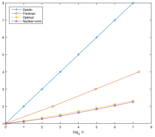
Figure 1: Bounds on $\gamma_{2}(T_{n})$: $\lceil\log_{2}n\rceil+1$ (top curve), Fredman’s factorization (second curve), the actual value computed by an SDP solver (third curve), and the lower bound $\frac{1}{n}\|T_{n}\|_{*}$. The $x$-axis shows $\log_{2}n$.

The resulting values of $\gamma_{2}(T_{n})$ are shown in Fig. 1, together with the $\lceil\log_{2}n\rceil+1$ upper bound and the lower bound of $\frac{1}{n}\|T_{n}\|_{*}$ as in Section 4.1. One can see that while $\frac{1}{n}\|T_{n}\|_{*}$ is quite a good approximation, it is not tight, and also that the upper bound $\lceil\log_{2}n\rceil+1$ overestimates the actual value almost four times. We have also plotted the value of $\|B\|_{2\to\infty}\|C\|_{1\to 2}$ for a factorization $T_{n}=BC$ due to Fredman [Fre82]; asymptotically, the value achieved by his method is $\log_{\lambda}n+O(\log\log n)$ for $\lambda=3+2\sqrt{2}$. Fredman’s factorization uses matrices with entries in $\{-1,0,1\}$ and it is asymptotically optimal over such factorizations with respect to $\max\{\|B\|_{2\to\infty},\|C\|_{1\to 2}\}$.

It would be interesting to find the exact value of $\gamma_{2}(T_{n})$ theoretically and to understand what the optimal ellipsoids look like. Fig. 2 shows a 3-dimensional plot of the entries of the dual matrix $D$ of an optimal ellipsoid for $T_{50}$; the two horizontal axes correspond to the rows and columns of $D$, and the vertical axis shows the magnitude of the entries. Similarly, in Fig. 3 we have plotted the diagonal entries of $P$ in an optimal solution $(P,Q)$ to the dual program in Theorem 2.4; the horizontal axis corresponds to an index $i$ and the vertical axis to the value $P_{ii}$. The diagonal entries of the optimal $Q$ appear to be identical to those of $P$ after a rearrangement: $Q_{ii}=P_{n-i+1,n-i+1}$. For both plots the values are defined for integer indexes only, and we have used interpolation to produce smooth graphs. It seems that, as $n\to\infty$, the matrices of the optimal ellipsoids should converge (in a suitable sense) to some nice function, and so should the optimal dual solutions, but we do not yet have a guess what these functions might be—they may very well be known in some area of mathematics.

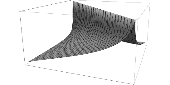
Figure 2: The dual matrix of an optimal ellipsoid for $T_{50}$.

Figure 3: Diagonal entries of an optimal dual solution for $T_{50}$.

5 General theorems about discrepancy

Union of set systems. Using the inequality in Lemma 2.6 and inequalities (1),(2), we obtain the following result, which is a somewhat sharper version of a theorem proved in [Mat13] using the determinant lower bound:

Theorem 5.1 (Union of set systems).

Let $\mathcal{F}_{1},\ldots,\mathcal{F}_{t}$ be set systems on an $n$-point ground set $V$, and let $\mathcal{F}=\mathcal{F}_{1}\cup\cdots\cup\mathcal{F}_{t}$. Then

$$\operatorname{herdisc}\mathcal{F}\leq O\Bigl{(}\sqrt{\log|\mathcal{F}|}\Bigr{)}\biggl{(}\sum_{i=1}^{t}(\log|\mathcal{F}_{i}|)^{2}(\operatorname{herdisc}\mathcal{F}_{i})^{2}\biggr{)}^{1/2}.$$

We note that if the set systems $\mathcal{F}_{1}$ and $\mathcal{F}_{2}$ have disjoint ground sets, then $\operatorname{herdisc}(\mathcal{F}_{1}\cup\mathcal{F}_{2})=\max(\operatorname{herdisc}\mathcal{F}_{1},\operatorname{herdisc}\mathcal{F}_{2})$, which can be regarded as a counterpart of Lemma 2.7.

Building sets from disjoint pieces. In a similar vein, the triangle inequality for $\gamma_{2}$ together with (1),(2) immediately yield the following consequence:

Theorem 5.2.

Let $\mathcal{F}_{1},\ldots,\mathcal{F}_{t}$ be set systems on an $n$-point ground set $V$, and let $\mathcal{F}$ be a set system such that for each $F\in\mathcal{F}$ there are pairwise disjoint sets $F_{1}\in\mathcal{F}_{1}$,…, $F_{t}\in\mathcal{F}_{t}$ so that $F=F_{1}\cup\cdots\cup F_{t}$. Then

$$\operatorname{herdisc}\mathcal{F}\leq O\Bigl{(}\sqrt{\log|\mathcal{F}|}\Bigr{)}\sum_{i=1}^{t}(\log|\mathcal{F}_{i}|)\operatorname{herdisc}\mathcal{F}_{i}.$$

In Section 6 below, we will obtain an example showing that if each of the systems $\mathcal{F}_{i}$ in the theorem has hereditary discrepancy at most $D$, the system $\mathcal{F}$ may have discrepancy about $tD$, up to a logarithmic factor, and thus in this sense, the theorem is not far from worst-case optimal.

Product set systems. Let $\mathcal{F}$ be a set system on a ground set $V$, and $\mathcal{G}$ a set system on a ground set $W$. Following Doerr, Srivastav, and Wehr [DSW04] (and probably many other sources), we define the product $\mathcal{F}\times\mathcal{G}$ as the set system $\{F\times G:F\in\mathcal{F},G\in\mathcal{G}\}$ on $V\times W$.

Since the incidence matrix of $\mathcal{F}\times\mathcal{G}$ is the Kronecker product of the incidence matrices of $\mathcal{F}$ and $\mathcal{G}$, from Theorem 2.3 and the usual inequalities (1),(2), we get that the hereditary discrepancy is approximately multiplicative:

Theorem 5.3.

Let $\mathcal{F}_{1},\ldots,\mathcal{F}_{t}$ be set systems, let $m_{i}=|\mathcal{F}_{i}|>1$ for all $i$, let $\mathcal{F}=\mathcal{F}_{1}\times\cdots\times\mathcal{F}_{t}$, and let $D:=\prod_{i=1}^{t}\operatorname{herdisc}\mathcal{F}_{i}$. Then

$$\frac{D}{C^{t}\log|\mathcal{F}|\prod_{i=1}^{t}\sqrt{\log m_{i}}}\leq\operatorname{herdisc}\mathcal{F}\leq D\cdot C^{t}\sqrt{\log|\mathcal{F}|}\prod_{i=1}^{t}\log m_{i}$$

with a suitable absolute constant $C$.

In the proof of the bounds for Tusnády’s problem in Section 6 we will see that the upper bound is not far from being tight. Here we give a simple example showing that the lower bound is near-tight as well.

Let $m=2^{k}$ with $k$ even and let $\mathcal{P}=2^{[k]}$ be the system of all subsets of the $k$-element set $[k]$. Then $|\mathcal{P}|=m$ and $\operatorname{herdisc}\mathcal{P}=k/2$. The lower bound in the theorem for the hereditary discrepancy of the $t$-fold product $\mathcal{P}^{t}$, assuming $t$ constant, is of order $D/\log^{t/2+1}m$, where $D=\operatorname{herdisc}(\mathcal{P})^{t}$. On the other hand, it is well known that any system of $M$ sets on $n$ points has discrepancy $O(\sqrt{n\log M}\,)$ (this is witnessed by a random coloring; see, e.g., [Spe87, Cha00, Mat10]), which in our case, with $n=k^{t}$ and $M=m^{t}$, shows that $\operatorname{herdisc}(\mathcal{P}^{t})$ is at most of order $k^{t/2+1/2}\approx D/(\log m)^{t/2-1/2}$, which differs from the lower bound only by a factor of $\log^{3/2}m$, independent of $t$.

6 On Tusnády’s problem

Proof of Theorem 1.1.

The proof was already sketched in the introduction, so here we just present it slightly more formally. Let $\mathcal{A}_{d}\subseteq\mathcal{R}_{d}$ be the set of all anchored axis-parallel boxes, of the form $[0,b_{1}]\times\cdots\times[0,b_{d}]$. Clearly $\operatorname{disc}(n,\mathcal{A}_{d})\leq\operatorname{disc}(n,\mathcal{R}_{d})$, and since every box $R\in\mathcal{R}_{d}$ can be expressed as a signed combination of at most $2^{d}$ anchored boxes, we have $\operatorname{disc}(n,\mathcal{R}_{d})\leq 2^{d}\operatorname{disc}(n,\mathcal{A}_{d})$.

Let us consider the $d$-dimensional grid $[n]^{d}\subset{\mathbb{R}}^{d}$ (with $n^{d}$ points), and let $\mathcal{G}_{d,n}=\mathcal{A}_{d}([n]^{d})$ be the subsets induced on it by anchored boxes. It suffices to prove that $\operatorname{herdisc}\mathcal{G}_{d,n}=\Omega(\log^{d-1}n)$, and for this, in view of inequality (1), it is enough to show that $\gamma_{2}(\mathcal{G}_{d,n})=\Omega(\log^{d}n)$.

Now $\mathcal{G}_{d,n}$ is (isomorphic to) the $d$-fold product $\mathcal{I}_{n}^{d}$ of the system of initial segments in $\{1,2,\ldots,n\}$, and so $\gamma_{2}(\mathcal{G}_{d,n})=\gamma_{2}(T_{n})^{d}=\Theta(\log^{d}n)$ (Theorem 2.3 and Proposition 4.1).

This finishes the proof of the lower bound. To prove the upper bound $\operatorname{disc}(n,\mathcal{R}_{d})=O(\log^{d+1/2}n)$, we consider an arbitrary $n$-point set $P\subset{\mathbb{R}}^{d}$. Since the set system $\mathcal{A}_{d}(P)$ is not changed by a monotone transformation of each of the coordinates, we may assume $P\subseteq[n]^{d}$. Hence

$$\operatorname{disc}(\mathcal{A}_{d}(P))\leq\operatorname{herdisc}\mathcal{G}_{d,n}\leq O(\gamma_{2}(\mathcal{G}_{d,n})\sqrt{\log n^{d}}\,)=O(\log^{d+1/2}n).$$

∎

Near-optimality of the bounds in Theorems 5.2 and 5.3. In Theorem 5.3 (discrepancy for the product of set systems), if we set $\mathcal{F}_{i}=\mathcal{I}_{m}$ for all $i=1,2,\ldots,t$, then the product of $\operatorname{herdisc}\mathcal{F}_{i}$ is $D=1$, while the hereditary discrepancy of the product is $\Omega(\log^{t-1}m)$ assuming $t$ constant. The upper bound in Theorem 5.3 is $O(\log^{t+1/2}m)$.

For Theorem 5.2 (sets made of disjoint pieces), we take $\mathcal{F}$ to be the set system $\mathcal{G}_{d,n}$ induced on the grid $[n]^{d}$ by anchored axis-parallel boxes, with hereditary discrepancy at least $\Omega(\log^{d-1}n)$.

To define the systems $\mathcal{F}_{i}$, we use canonical binary boxes. First let us define a (binary) canonical interval in $[n]$ as a set of the form $I=[a2^{i},(a+1)2^{i})\cap[n]$, with $i$ and $a$ nonnegative integers. Let us call $2^{i}$ the size of such a canonical interval. As is well known, and easy to see, every initial interval $J=\{1,2,\ldots,j\}\subseteq[n]$ can be expressed as a disjoint union of canonical intervals, with at most one canonical intervals for every size (and consequently, there are $O(\log n)$ canonical intervals in the union).

Next, a canonical box in $[n]^{d}$ is a product $B=I_{1}\times\cdots\times I_{d}$ of canonical intervals. The size of $B$ is the $d$-tuple $(2^{i_{1}},\ldots,2^{i_{d}})$, where $2^{i_{j}}$ is the size of $I_{j}$. Clearly, every set in $\mathcal{G}_{d,n}$ is a disjoint union of $O(\log^{d}n)$ canonical boxes, at most one for every possible size.

Let $T$ be the set of all sizes of canonical boxes, $|T|=\Theta(\log^{d}n)$, and for every size $s\in T$, let $\mathcal{B}_{s}$ be the system of all canonical boxes of size $s$, plus the empty set. By the above, each set of $\mathcal{G}_{d,n}$ is a disjoint union $\bigcup_{s\in T}B_{s}$ for some $B_{s}\in\mathcal{B}_{s}$, and so the $\mathcal{B}_{s}$ can play the role of the $\mathcal{F}_{i}$ in Theorem 5.2, with $t=|T|$.

We have $D=\operatorname{herdisc}\mathcal{B}_{s}=1$ for every $s$ (since the canonical boxes of a given size are pairwise disjoint), and so $\operatorname{herdisc}\mathcal{G}_{d,n}=\Omega(t^{1-1/d})D$ for every constant $d$. Hence if, in the setting of Theorem 5.2, $D=\max\operatorname{herdisc}\mathcal{F}_{i}$, we cannot bound $\operatorname{herdisc}\mathcal{F}$ by $O(t^{1-\delta}(\log|\mathcal{F}|)^{c}D)$ for any fixed $c$ and $\delta>0$ (unlike for the union of set systems in Theorem 5.1, where the bound is roughly $\sqrt{t}\cdot D$, up to a logarithmic factor).

6.1 Discrepancy of boxes in high dimension

Chazelle and Lvov [CL01a, CL01b] investigated the hereditary discrepancy of the set system $\mathcal{C}_{d}:=\mathcal{R}_{d}(\{0,1\}^{d})$, the set system induced by axis-parallel boxes on the $d$-dimensional Boolean cube $\{0,1\}^{d}$. In other words, the sets in $\mathcal{C}_{d}$ are subcubes of $\{0,1\}^{d}$. Unlike for Tusnády’s problem where $d$ was considered fixed, here one is interested in the asymptotic behavior as $d\to\infty$.

Chazelle and Lvov proved $\operatorname{herdisc}\mathcal{C}_{d}=\Omega(2^{cd})$ for an absolute constant $c\approx 0.0477$, which was later improved to $c=0.0625$ in [NT13] (in relation to the hereditary discrepancy of homogeneous arithmetic progressions). Here we obtain an optimal value of the constant $c$:

Theorem 6.1.

The system $\mathcal{C}_{d}$ of subcubes of the $d$-dimensional Boolean cube satisfies

$$\operatorname{herdisc}\mathcal{C}_{d}=2^{c_{0}d+o(d)},$$

where $c_{0}=\log_{2}(2/\sqrt{3})\approx 0.2075$. The same bound holds for the system $\mathcal{A}_{d}(\{0,1\}^{d})$ of all subsets of the cube induced by anchored boxes.

Proof.

The number of sets in $\mathcal{C}_{d}$ is $3^{d}$, and so in view of inequalities (1) and (2) it suffices to prove $\gamma_{2}(\mathcal{C}_{d})=\gamma_{2}(\mathcal{A}_{d}(\{0,1\}^{d}))=2^{c_{0}d}$.

The system $\mathcal{C}_{d}$ is the $d$-fold product $\mathcal{C}_{1}^{d}$, and so by Theorem 2.3, $\gamma_{2}(\mathcal{C}_{d})=\gamma_{2}(\mathcal{C}_{1})^{d}$. The incidence matrix of $\mathcal{C}_{1}$ is

$$A=\begin{pmatrix}1&1\\ 1&0\\ 0&1\end{pmatrix}.$$

To get an upper bound on $\gamma_{2}(A)$, we exhibit an appropriate ellipsoid; it is more convenient to do it for $A^{T}$, since this is a planar problem. The optimal ellipse containing the rows of $A$ is $\{x\in{\mathbb{R}}^{2}:x_{1}^{2}+x_{2}^{2}-x_{1}x_{2}\leq 1\}$; here are a picture and the dual matrix:

$$\raisebox{-42.67912pt}{\includegraphics{subcubesEll}}\ \ \ \ \ \ \ \ \ \ \ \ D=\begin{pmatrix}\frac{4}{3}&\frac{1}{3}\\[2.84526pt] \frac{1}{3}&\frac{4}{3}\end{pmatrix}.$$

Hence $\gamma_{2}(A)\leq 2/\sqrt{3}$. The same ellipse also works for the incidence matrix of the system $\mathcal{A}_{1}(\{0,1\})$, which is the familiar lower triangular matrix $T_{2}$.

There are several ways of bounding $\gamma_{2}(T_{2})\leq\gamma_{2}(A)$ from below. For example, we can use Theorem 2.4 with

$$P=\begin{pmatrix}\frac{1}{3}&0\\[2.84526pt] 0&\frac{2}{3}\end{pmatrix},\ \ \ Q=\begin{pmatrix}\frac{2}{3}&0\\[2.84526pt] 0&\frac{1}{3}\end{pmatrix}.$$

With some effort (or a computer algebra system) one can check that the singular values of $P^{1/2}T_{2}Q^{1/2}$ are $\frac{1}{\sqrt{3}}\pm\frac{1}{3}$, and hence the nuclear norm is $2/\sqrt{3}$ as needed.

Alternatively, one can also check the optimality of the ellipse above by elementary geometry, or exhibit an optimal solution of the dual semidefinite program for $\gamma_{2}(T_{2})$. ∎

7 On combinatorial $L_{p}$-discrepancy

$L_{p}$-discrepancy in the continuous setting. Roth’s beautiful argument [Rot54] for the lower bound $D(n,\mathcal{R}_{d})=\Omega(\log^{(d-1)/2}n)$ actually bounds the discrepancy of an average anchored axis-parallel box. More precisely, Roth introduced the $p=2$ case of the following notion of $L_{p}$-discrepancy of an $n$-point set $P\subset[0,1]^{d}$ with respect to anchored boxes, defined by

$$D_{p}(P,\mathcal{A}_{d}):=\left(\int_{[0,1]^{d}}{\Bigl{|}|P\cap A(x)|-\lambda^{d}(A(x))\Bigr{|}^{p}dx}\right)^{1/p},$$

where $A(x):=[0,x_{1}]\times\ldots\times[0,x_{d}]$. This kind of discrepancy has also been investigated extensively since then, and its importance, e.g. for the theory of numerical integration, is comparable to the original “worst–case” discrepancy $D(P,\mathcal{R}_{d})$.

While the asymptotic behavior of $D(n,\mathcal{R}_{d})$ remains a mystery, it turns out that the $L_{p}$-discrepancy $D_{p}(n,\mathcal{A}_{d})$ is of order $\log^{(d-1)/2}n$ for every fixed $p$ and $d$, matching Roth’s lower bound. This was shown by Davenport [Dav56] for $d=p=2$, by Roth [Rot80] for $p=2$ and all $d$, and by Chen [Che80] (for all $p$).

Combinatorial $L_{p}$-discrepancy. A similar kind of average discrepancy can also be considered in the combinatorial setting, as was done, e.g., in [Sri97, Mat98]. Namely, for a set system $\mathcal{F}$ on the ground set $[n]$ we set

$$\operatorname{disc}_{p}\mathcal{F}:=\min_{x\in\{-1,1\}^{n}}\biggl{(}\frac{1}{|\mathcal{F}|}\sum_{F\in\mathcal{F}}|x(F)|^{p}\biggr{)}^{1/p},$$

with $x(F)=\sum_{j\in F}x_{j}$. More generally, for a nonnegative weight function $w\colon\mathcal{F}\to[0,\infty)$, not identically $0$, we similarly define

$$\operatorname{disc}_{p,w}\mathcal{F}:=\min_{x\in\{-1,1\}^{n}}\biggl{(}\tfrac{1}{w(\mathcal{F})}\sum_{F\in\mathcal{F}}w(F)|x(F)|^{p}\biggr{)}^{1/p}.$$

In this section we provide some general results concerning the combinatorial $L_{p}$-discrepancy, and we establish a lower bound for anchored boxes (an $L_{p}$-version of Tusnády’s problem).

For a point set $P\subset[0,1]^{d}$, we let $\mathcal{A}_{d}(P)$ be the system of all intersections of $P$ with anchored boxes as before, and let $\overline{w}=\overline{w}_{P}\colon\mathcal{A}_{d}(P)\to[0,1]$ be the weight function given by $\overline{w}(F):=\lambda^{d}\{x\in[0,1]^{d}:A(x)\cap P=F\}$; that is, the weight of a subset of $P$ is the Lebesgue measure of the set of all corners $x$ whose corresponding anchored boxes $A(x)$ intersect $P$ in $F$.

Theorem 7.1.

For every fixed $d\geq 2$ and infinitely many values of $n$, there is an $n$-point set $P\subset{\mathbb{R}}^{d}$ such that

$$\operatorname{disc}_{2,\overline{w}}\mathcal{A}_{d}(P)=\Omega(\log^{d-1}n).$$

Thus, the combinatorial $L_{2}$-discrepancy for axis-parallel anchored boxes has the same lower bound as the worst-case discrepancy, and it is roughly the square of the $L_{2}$-discrepancy in the Lebesgue-measure case. (Admittedly, the analogy between the $L_{2}$-discrepancy in the Lebesgue-measure and combinatorial cases is far from perfect.)

We start working towards the proof of the theorem. First we extend the definition of $L_{p}$-discrepancy to matrices in a natural way: for an $m\times n$ matrix $A$ we set

$$\operatorname{disc}_{p}A:=\min_{x\in\{-1,1\}^{n}}m^{-1/p}\|Ax\|_{p}.$$

The hereditary analog, $\operatorname{herdisc}_{p}A$, is naturally defined as $\max_{J\subseteq[n]}\operatorname{disc}_{p}A_{J}$.

Now let us consider a weight function $w\colon[m]\to[0,\infty)$ on the rows of $A$. It is useful to observe that the corresponding weighted $L_{p}$-discrepancy of $A$ can be written using the unweighted discrepancy of $A$ suitably modified—namely, the $i$th row needs to be multiplied by $w(i)^{1/p}$, assuming $w$ normalized so that $\sum_{i=1}^{m}w(i)=m$. Then, with this normalization of $w$ and with $W:=\operatorname{diag}(w)$ being the $m\times m$ matrix with the $w(i)$ on the diagonal, we can write

$$\operatorname{disc}_{p,w}A=\operatorname{disc}_{p}W^{1/p}A.$$

Let us consider the following $L_{2}$-version of the determinant lower bound:

$$\operatorname{detlb}_{2}A:=\max_{J:\emptyset\neq J\subseteq[n]}\sqrt{|J|/m}\cdot|\det A_{J}^{T}A_{J}|^{1/2|J|}.$$

The following is proved in the journal version of [NTZ13] by an easy modification of the argument of Lovász et al. [LSV86]:

Lemma 7.2.

There exists a constant $c>0$ such that for every $m\times n$ matrix $A$,

$$\operatorname{herdisc}_{2}\geq c\operatorname{detlb}_{2}A.$$

We use this lemma, together with a modification of our proof of inequality (1), to establish the following:

Lemma 7.3.

Let $A$ be an $m\times n$ matrix, let $w\colon[m]\to[0,\infty)$ be a nonnegative weight function on the rows normalized so that $\sum_{i=1}^{m}w(i)=m$, and let $P=\frac{1}{m}\operatorname{diag}(w)$. Then for every nonnegative diagonal matrix $Q$ with unit trace we have

$$\|P^{1/2}AQ^{1/2}\|_{*}=O(\log m)\operatorname{herdisc}_{2,w}A.$$

Proof.

In the proof of Theorem 3.1, we showed that if $Q$ is a non-negative diagonal unit-trace matrix, then there exists a submatrix $D=P^{1/2}A_{J}$ of $P^{1/2}A$ such that

$$|\det D^{T}D|^{1/2k}=\Omega\left(\frac{1}{\sqrt{k}\log m}\right)\|P^{1/2}AQ^{1/2}\|_{*},$$

where $k:=|J|$. Setting $W:=mP$ and $\tilde{A}:=W^{1/2}A$, the matrix $\sqrt{m}\cdot D$ is a witness for $\operatorname{detlb}_{2}\tilde{A}=\Omega(1/\log m)\cdot\|P^{1/2}AQ^{1/2}\|_{*}$. The lemma then follows by applying Lemma 7.2 to the matrix $\tilde{A}$. ∎

Proof of Theorem 7.1.

In the proof of Theorem 1.1 we have shown that $\gamma_{2}(\mathcal{G}_{d,n})=\Omega(\log^{d}n)$, where $\mathcal{G}_{d,n}=\mathcal{A}_{d}([n]^{d})$ is the set system induced by anchored boxes on the grid $[n]^{d}$. Unwrapping the proof shows that the diagonal matrices $P$ and $Q$ witnessing the lower bound on $\gamma_{2}(\mathcal{G}_{d,n})$ via Theorem 2.4 can actually be taken uniform, i.e., $P=Q=\frac{1}{N}I_{N}$, $N=n^{d}$.

Therefore, applying Lemma 7.3 with $A$ the incidence matrix of $\mathcal{G}_{d,n}$, $P=\frac{1}{N}I_{N}$, and $w\equiv 1$ the uniform weight function, we obtain $\operatorname{herdisc}_{2}A=\Omega(\log^{d-1}n)$. The theorem then follows from the definition of $\operatorname{herdisc}_{2}A$ (one can check that the weights of the subsets are given by $\overline{w}$ as in the theorem after appropriately scaling and shifting the grid $[n]^{d}$). ∎

8 Simple proofs of known discrepancy bounds

The properties of the $\gamma_{2}$ norm allow for surprisingly easy proofs of some known bounds in discrepancy theory; we have already seen this in the case of the upper bound for Tusnády’s problem. Here we add some more examples, where we obtain slightly suboptimal results.

For convenience, we first summarize the required properties.

1. (Herdisc and $\gamma_{2}$) $\frac{\gamma_{2}(A)}{O(\log m)}\leq\operatorname{herdisc}A\leq\gamma_{2}(A)\cdot O(\sqrt{\log m})$; these are inequalities (1), (2).

2. (Degree bound) If each point in a set system $\mathcal{F}$ is in at most $t$ sets, then $\gamma_{2}(\mathcal{F})\leq\sqrt{t}$. (This is because the columns of the incidence matrix $A$ are contained in the ball of radius $\sqrt{t}$, or, equivalently, by the trivial factorization $A=IA$.)

3. (Size bound) If all sets of $\mathcal{F}$ have size at most $t$, then $\gamma_{2}(\mathcal{F})\leq\sqrt{t}$. (This is (B) and Lemma 2.1, or, equivalently, by the factorization $A=AI$.)

4. (Union) If $\mathcal{F}=\mathcal{F}_{1}\cup\cdots\cup\mathcal{F}_{t}$, then $\gamma_{2}(\mathcal{F})\leq\bigl{(}\sum_{i=1}^{t}\gamma_{2}(\mathcal{F}_{i})^{2}\bigr{)}^{1/2}$ (Lemma 2.6).

5. (Disjoint supports) If set systems $\mathcal{F}_{1}$ and $\mathcal{F}_{2}$ have disjoint ground sets, then $\gamma_{2}(\mathcal{F}_{1}\cup\mathcal{F}_{2})=\max(\gamma_{2}(\mathcal{F}_{1}),\gamma_{2}(\mathcal{F}_{2}))$ (Lemma 2.7).

6. (Sets from disjoint pieces) If every set $F\in\mathcal{F}$ can be written as a disjoint union $F_{1}\cup\cdots\cup F_{t}$, $F_{i}\in\mathcal{F}_{i}$, then $\gamma_{2}(\mathcal{F})\leq\sum_{i=1}^{t}\gamma_{2}(\mathcal{F}_{i})$.

7. (Product) $\gamma_{2}(\mathcal{F}_{1}\times\mathcal{F}_{2})=\gamma_{2}(\mathcal{F}_{1})\times\gamma_{2}(\mathcal{F}_{2})$.

A bound in terms of the maximum degree. If $\mathcal{F}$ has maximum degree $t$, i.e., no point is in more than $t$ sets, then we get $\operatorname{disc}\mathcal{F}=O(\sqrt{t\log m})$ by (A) and (B), which recovers the current best bound for this problem, due to Banaszczyk [Ban98]. However, this example is not quite fair, since inequality (2) used in (A) relies on a more general form of Banaszczyk’s estimate.

The $k$-permutation problem. Given a permutation $\pi$ of $\{1,2,\ldots,n\}$, we consider the system $\mathcal{P}_{\pi}$ of all initial segments along $\pi$, i.e., the sets $\{\pi(1),\ldots,\pi(i)\}$, $i=1,2,\ldots,n$. The $k$-permutation problem asks for the maximum discrepancy of $\mathcal{P}:=\mathcal{P}_{\pi_{1}}\cup\cdots\cup\mathcal{P}_{\pi_{k}}$, where $\pi_{1},\ldots,\pi_{k}$ are $k$ permutations of $\{1,2,\ldots,n\}$. For $k\geq 3$, the best known upper bound is $O(\sqrt{k}\cdot\log n)$ [Sri97], and it is sharp for $k\geq 3$ fixed [NNN12].

As is well known, $\operatorname{herdisc}\mathcal{P}_{\pi}\leq 1$ for every $\pi$, and so (A) and (C) give $\operatorname{disc}\mathcal{P}=O(\sqrt{k}\cdot\log^{3/2}n)$.

Arithmetic progressions. Let $\mathcal{AP}$ be the system of all arithmetic progressions on the set $\{1,2,\ldots,n\}$. The discrepancy of $\mathcal{AP}$ was considered in a classical paper of Roth [Rot64], who proved an $\Omega(n^{1/4})$ lower bound. A matching upper bound of $O(n^{1/4})$ was obtained in [MS96], after previous weaker results by several authors.

First we present a quick way of obtaining the slightly worse upper bound of $O(n^{1/4}\log n)$. Let $\mathcal{AP}_{d}\subseteq\mathcal{AP}$ consist of all arithmetic progressions with difference exactly $d$. Obviously $\operatorname{herdisc}\mathcal{AP}_{d}\leq 1$ for all $d$, and so $\gamma_{2}(\mathcal{AP}_{d})=O(\log n)$ by (A). Let us set $\mathcal{AP}_{\geq s}:=\bigcup_{d\geq s}\mathcal{AP}_{d}$. Since all sets in $\mathcal{AP}_{\geq s}$ have size at most $n/s$, we have $\gamma_{2}(\mathcal{AP}_{\geq s})=O(\sqrt{n/s}\,)$ by (B^′). So, for every $s$, $\gamma_{2}(\mathcal{AP})^{2}\leq\sum_{d=1}^{s-1}\gamma_{2}(\mathcal{AP}_{d})^{2}+\gamma_{2}(\mathcal{AP}_{\geq s})^{2}=O(s\log^{2}n+n/s)$ according to (C). Minimizing with $s:=\sqrt{n}/\log n$ gives $\gamma_{2}(\mathcal{AP})=O(n^{1/4}\sqrt{\log n})$, and thus $\operatorname{disc}\mathcal{AP}=O(n^{1/4}\log n)$ by (A).

A more careful analysis, combining the ideas above with the canonical intervals trick, shows an asymptotically optimal bound for $\gamma_{2}(\mathcal{AP})$, which in turn implies $\operatorname{herdisc}\mathcal{AP}=O(n^{1/4}\sqrt{\log n}\,)$, a better but still suboptimal bound.

Proposition 8.1.

$\gamma_{2}(\mathcal{AP})=\Theta(n^{1/4})$.

Proof.

The lower bound $\gamma_{2}(\mathcal{AP})=\Omega(n^{1/4})$ is implied by the Lovász’ proof of Roth’s $1/4$-theorem using eigenvalues; see [BS95] or [Cha00, Sec. 1.5]. That proof provides a square matrix $\tilde{A}$ in which each row is the sum of the indicator vectors of at most two disjoint arithmetic progressions in $[n]$, and such that the smallest singular value $\sigma_{\min}$ of $\tilde{A}$ is of order $\Omega(n^{1/4})$.

By the triangle inequality (and since removing rows does not increase $\gamma_{2}$), we have $\gamma_{2}(\mathcal{AP})\geq\frac{1}{2}\gamma_{2}(\tilde{A})$. Then $\gamma_{2}(\tilde{A})\geq\frac{1}{n}\|\tilde{A}\|_{*}\geq\sigma_{\min}=\Omega(n^{1/4})$, which proves the lower bound.

Next, we do the upper bound. For an interval $I\subseteq[n]$, let $\mathcal{M}_{I}$ be the set of all inclusion-maximal arithmetic progressions in $I$. We claim that

$$\gamma_{2}(\mathcal{M}_{I})\leq\sqrt{2}|I|^{1/4}.$$ (6)

Before proving (6), let us see why it implies $\gamma_{2}(\mathcal{AP})=O(n^{1/4})$. We recall that a binary canonical interval of size $2^{i}$ is an interval of the form $I=[a2^{i},(a+1)2^{i})\cap[n]$, where $a$ and $i$ are natural numbers. Let $\mathcal{M}_{i}$ be the union of the set systems $\mathcal{M}_{I}$ over all canonical intervals $I$ of size $2^{i}$. Since $\mathcal{M}_{i}$ is a union of set systems with disjoint supports, by (D) and (6), $\gamma_{2}(\mathcal{M}_{i})\leq 2^{\frac{i}{4}+\frac{1}{2}}$.

Every arithmetic progression in $[n]$ can be written as the disjoint union of arithmetic progressions from $\mathcal{M}_{0},\ldots,\mathcal{M}_{k}$, $k=\lfloor\log_{2}n\rfloor$, so that at most two maximal arithmetic progressions from each $\mathcal{M}_{i}$ are taken. Property (E) then gives $\gamma_{2}(\mathcal{AP})\leq\sum_{i=0}^{k}{2\cdot 2^{\frac{i}{4}+\frac{1}{2}}}=O(n^{1/4})$.

It remains to prove (6). Let us split $\mathcal{M}_{I}$ as $\mathcal{M}_{I}^{\prime}\cup\mathcal{M}^{\prime\prime}_{I}$, where the arithmetic progressions in $\mathcal{M}_{I}^{\prime}$ have difference at most $|I|^{1/2}$, and those in $\mathcal{M}_{I}^{\prime\prime}$ have difference larger than $|I|^{1/2}$.

Given a difference $d$, each $c\in I$ belongs to exactly one maximal arithmetic progression with difference $d$, because such an arithmetic progression is entirely determined by the congruence class of $c\bmod d$. Therefore, each integer in $I$ belongs to at most $|I|^{1/2}$ arithmetic progressions in $\mathcal{M}_{I}^{\prime}$, and, by (B), $\gamma_{2}(\mathcal{M}_{I}^{\prime})\leq|I|^{1/4}$.

On the other hand, every arithmetic progression in $\mathcal{M}_{I}^{\prime\prime}$ has size at most $|I|^{1/2}$, and so, by (B^′), $\gamma_{2}(\mathcal{M}_{I}^{\prime\prime})\leq|I|^{1/4}$ as well. Since $\mathcal{M}_{I}=\mathcal{M}_{I}^{\prime}\cup\mathcal{M}_{I}^{\prime\prime}$, we have $\gamma_{2}(\mathcal{M}_{I})\leq\sqrt{2}|I|^{1/4}$ as desired. ∎

Multidimensional arithmetic progressions. Doerr, Srivastav, and Wehr [DSW04] considered the discrepancy of the system $\mathcal{AP}^{d}$ of $d$-dimensional arithmetic progressions in $[n]^{d}$, which are $d$-fold Cartesian products of arithmetic progressions. They showed that $\operatorname{disc}\mathcal{AP}^{d}=\Theta(n^{d/4})$.

Their upper bound was done by a simple product coloring argument, which does not apply to hereditary discrepancy (since the restriction of $\mathcal{AP}^{d}$ to a subset of $[n]^{d}$ no longer has the structure of multidimensional arithmetic progressions). By Proposition 8.1 and (F) we have $\gamma_{2}(\mathcal{AP}^{d})=\Theta(n^{d/4})$, and we thus obtain the (probably suboptimal) upper bound $\operatorname{herdisc}\mathcal{AP}^{d}=O(n^{d/4}\sqrt{\log n}\,)$.

The lower bound in [DSW04] uses a nontrivial Fourier-analytic argument. Here we observe that it also follows from Lovász’ lower bound proof for $\operatorname{disc}\mathcal{AP}$ mentioned above, and a product argument. Indeed, the $d$-fold Kronecker product $\tilde{A}^{\otimes d}$ of the matrix $\tilde{A}$ as in the proof of Proposition 8.1 has the smallest singular value $\sigma_{\min}^{d}=\Omega(n^{d/4})$ for every fixed $d$, and each of its rows is the indicator vector of the disjoint union of at most $2^{d}$ sets of $\mathcal{AP}^{d}$. So $\operatorname{disc}\mathcal{AP}^{d}\geq 2^{-d}\operatorname{disc}\tilde{A}^{\otimes d}=\Omega(n^{d/4})$, where the final equality is by the well-known fact that the smallest singular value is a lower bound on the discrepancy of a square matrix (see [Mat10, Sec. 4.2] or [Cha00, Sec. 1.5]).

Acknowledgments

We would like to thank Alan Edelman and Gil Strang for invaluable advice concerning the singular values of the matrix in Proposition 4.1, and Van Vu for recommending the right experts for this question. We would also like to thank Noga Alon and Assaf Naor for pointing out that the geometric quantity in [NT15, MN14] is equivalent to the $\gamma_{2}$ norm. We also thank Imre Bárány and Vojtěch Tuma for useful discussions.

References

- [ABC97] J. R. Alexander, J. Beck, and W. W. L. Chen. Geometric discrepancy theory and uniform distribution. In J. E. Goodman and J. O’Rourke, editors, Handbook of Discrete and Computational Geometry, chapter 10, pages 185–207. CRC Press LLC, Boca Raton, FL, 1997.
- [AE45] T. van Aardenne-Ehrenfest. Proof of the impossibility of a just distribution of an infinite sequence of points. Nederl. Akad. Wet., Proc., 48:266–271, 1945. Also in Indag. Math. 7, 71-76 (1945).
- [AE49] T. van Aardenne-Ehrenfest. On the impossibility of a just distribution. Nederl. Akad. Wet., Proc., 52:734–739, 1949. Also in Indag. Math. 11, 264-269 (1949).
- [Bal97] K. Ball. An elementary introduction to modern convex geometry. In S. Levi, editor, Flavors of Geometry (MSRI Publications vol. 31), pages 1–58. Cambridge University Press, Cambridge, 1997.
- [Bal01] Keith Ball. Convex geometry and functional analysis. In Handbook of the geometry of Banach spaces, Vol. I, pages 161–194. North-Holland, Amsterdam, 2001.
- [Ban98] W. Banaszczyk. Balancing vectors and Gaussian measures of -dimensional convex bodies. Random Structures and Algorithms, 12(4):351–360, 1998.
- [Ban10] N. Bansal. Constructive algorithms for discrepancy minimization. http://arxiv.org/abs/1002.2259, also in FOCS’10: Proc. 51st IEEE Symposium on Foundations of Computer Science, pages 3–10, 2010.
- [BC87] J. Beck and W. W. L. Chen. Irregularities of Distribution. Cambridge University Press, Cambridge, 1987.
- [Bec81] J. Beck. Balanced two-colorings of finite sets in the square. I. Combinatorica, 1:327–335, 1981.
- [Bec89a] J. Beck. Balanced two-colorings of finite sets in the cube. Discrete Mathematics, 73:13–25, 1989.
- [Bec89b] J. Beck. A two-dimensional van Aardenne-Ehrenfest theorem in irregularities of distribution. Compositio Math., 72:269–339, 1989.
- [Bha97] Rajendra Bhatia. Matrix analysis, volume 169 of Graduate Texts in Mathematics. Springer-Verlag, New York, 1997.
- [BL08] D. Bilyk and M. T. Lacey. On the small ball inequality in three dimensions. Duke Math. J., 143(1):81–115, 2008.
- [BLV08] D. Bilyk, M. T. Lacey, and A. Vagharshakyan. On the small ball inequality in all dimensions. J. Funct. Anal., 254(9):2470–2502, 2008.
- [Boh90] G. Bohus. On the discrepancy of 3 permutations. Random Struct. Algo., 1:215–220, 1990.
- [BS95] J. Beck and V. Sós. Discrepancy theory. In Handbook of Combinatorics, pages 1405–1446. North-Holland, Amsterdam, 1995.
- [Cha00] B. Chazelle. The Discrepancy Method. Cambridge University Press, Cambridge, 2000.
- [Che80] W. W. L. Chen. On irregularities of distribution. Mathematika, 27:153–170, 1980.
- [CL01a] B. Chazelle and A. Lvov. A trace bound for the hereditary discrepancy. Discrete Comput. Geom., 26(2):221–231, 2001.
- [CL01b] B. Chazelle and A. Lvov. The discrepancy of boxes in higher dimension. Discrete Comput. Geom., 25(4):519–524, 2001.
- [CNN11] M. Charikar, A. Newman, and A. Nikolov. Tight hardness results for minimizing discrepancy. In Proc. 22nd Annual ACM-SIAM Symposium on Discrete Algorithms (SODA), San Francisco, California, USA, pages 1607–1614, 2011.
- [Cor35a] J. G. van der Corput. Verteilungsfunktionen I. Akad. Wetensch. Amsterdam, Proc., 38:813–821, 1935.
- [Cor35b] J. G. van der Corput. Verteilungsfunktionen II. Akad. Wetensch. Amsterdam, Proc., 38:1058–1066, 1935.
- [Dav56] H. Davenport. Note on irregularities of distribution. Mathematika, 3:131–135, 1956.
- [DSW04] B. Doerr, A. Srivastav, and P. Wehr. Discrepancy of Cartesian products of arithmetic progressions. Electron. J. Combin., 11:Research Paper 5, 16 pp. (electronic), 2004.
- [DT97] M. Drmota and R. F. Tichy. Sequences, discrepancies and applications (Lecture Notes in Mathematics 1651). Springer-Verlag, Berlin etc., 1997.
- [Fre82] Michael L. Fredman. The complexity of maintaining an array and computing its partial sums. J. ACM, 29(1):250–260, 1982.
- [FSS01] Jürgen Forster, Niels Schmitt, and Hans Ulrich Simon. Estimating the optimal margins of embeddings in Euclidean half spaces. In Computational learning theory (Amsterdam, 2001), volume 2111 of Lecture Notes in Comput. Sci, pages 402–415. Springer, Berlin, 2001.
- [GLS88] M. Grötschel, L. Lovász, and A. Schrijver. Geometric Algorithms and Combinatorial Optimization, volume 2 of Algorithms and Combinatorics. Springer-Verlag, Berlin etc., 1988. 2nd edition 1993.
- [Hal60] J. H. Halton. On the efficiency of certain quasi-random sequences of points in evaluating multi-dimensional integrals. Numer. Math., 2:84–90, 1960.
- [Ham60] J. M. Hammersley. Monte Carlo methods for solving multivariable problems. Ann. New York Acad. Sci., 86:844–874, 1960.
- [Lar14] K. G. Larsen. On range searching in the group model and combinatorial discrepancy. SIAM Journal on Computing, 43(2):673–686, 2014.
- [LMSS07] Nati Linial, Shahar Mendelson, Gideon Schechtman, and Adi Shraibman. Complexity measures of sign matrices. Combinatorica, 27(4):439–463, 2007.
- [LS09a] Nati Linial and Adi Shraibman. Learning complexity vs. communication complexity. Combin. Probab. Comput., 18(1-2):227–245, 2009.
- [LS09b] Nati Linial and Adi Shraibman. Lower bounds in communication complexity based on factorization norms. Random Structures Algorithms, 34(3):368–394, 2009.
- [LSŠ08] Troy Lee, Adi Shraibman, and Robert Špalek. A direct product theorem for discrepancy. In Proceedings of the 23rd Annual IEEE Conference on Computational Complexity, CCC 2008, 23-26 June 2008, College Park, Maryland, USA, pages 71–80. IEEE Computer Society, 2008.
- [LSV86] L. Lovász, J. Spencer, and K. Vesztergombi. Discrepancy of set-systems and matrices. European J. Combin., 7:151–160, 1986.
- [Mat98] J. Matoušek. An version of the Beck-Fiala conjecture. European J. Combinatorics, 19:175–182, 1998.
- [Mat99] J. Matoušek. On the discrepancy for boxes and polytopes. Monatsh. Math., 127(4):325–336, 1999.
- [Mat10] J. Matoušek. Geometric Discrepancy (An Illustrated Guide), 2nd printing. Springer-Verlag, Berlin, 2010.
- [Mat13] J. Matoušek. The determinant bound for discrepancy is almost tight. Proc. Amer. Math. Soc., 141(2):451–460, 2013.
- [MN12] S. Muthukrishnan and A. Nikolov. Optimal private halfspace counting via discrepancy. In STOC ’12: Proceedings of the 44th symposium on Theory of Computing, pages 1285–1292, New York, NY, USA, 2012. ACM.
- [MN14] J. Matoušek and A. Nikolov. Combinatorial discrepancy for boxes via the ellipsoid-infinity norm. Preprint at arXiv:1408.1376, to appear in SoCG 15 as ”Combinatorial discrepancy for boxes via the norm”, 2014.
- [MS96] J. Matoušek and J. Spencer. Discrepancy in arithmetic progressions. J. Amer. Math. Soc., 9:195–204, 1996.
- [NNN12] A. Newman, O. Neiman, and A. Nikolov. Beck’s three permutations conjecture: A counterexample and some consequences. In Proc. 53rd Annual IEEE Symposium on Foundations of Computer Science (FOCS), pages 253–262, 2012.
- [NT13] A. Nikolov and K. Talwar. On the hereditary discrepancy of homogeneous arithmetic progressions. Proc. Amer. Math. Soc., 2013. To appear. Preprint at arXiv:1309:6034.
- [NT15] A. Nikolov and K. Talwar. Approximating hereditary discrepancy via small width ellipsoids. In Proc. 26th ACM-SIAM Symposium on Discrete Algorithms, pages 324–336. SIAM, 2015.
- [NTZ13] A. Nikolov, K. Talwar, and Li Zhang. The geometry of differential privacy: the sparse and approximate cases. In Proc. 45th ACM Symposium on Theory of Computing (STOC), Palo Alto, California, USA, pages 351–360, 2013. Full version to appear in SIAM Journal on Computing as The Geometry of Differential Privacy: the Small Database and Approximate Cases.
- [Pál10] D. Pálvölgyi. Indecomposable coverings with concave polygons. Discrete Comput. Geom., 44(3):577–588, 2010.
- [Rot54] K. F. Roth. On irregularities of distribution. Mathematika, 1:73–79, 1954.
- [Rot64] K. F. Roth. Remark concerning integer sequences. Acta Arith., 9:257–260, 1964.
- [Rot80] K. F. Roth. On irregularities of distribution IV. Acta Arith., 37:67–75, 1980.
- [Rot14] Thomas Rothvoß. Constructive discrepancy minimization for convex sets. CoRR, abs/1404.0339, 2014. To Appear in FOCS 2014.
- [Sch72] W. M. Schmidt. On irregularities of distribution VII. Acta Arith., 21:45–50, 1972.
- [See93] A. Seeger. Calculus rules for combinations of ellipsoids and applications. Bull. Australian Math. Soc., 47(01):1–12, 1993.
- [SM14] G. Strang and S. MacNamara. Functions of difference matrices are Toeplitz plus Hankel. SIAM Review, 2014. To appear.
- [Spe87] J. Spencer. Ten Lectures on the Probabilistic Method. CBMS-NSF. SIAM, Philadelphia, PA, 1987.
- [Sri97] A. Srinivasan. Improving the discrepancy bound for sparse matrices: better approximations for sparse lattice approximation problems. In Proc. 8th ACM-SIAM Symposium on Discrete Algorithms, pages 692–701, 1997.
- [TJ89] Nicole Tomczak-Jaegermann. Banach-Mazur distances and finite-dimensional operator ideals, volume 38 of Pitman Monographs and Surveys in Pure and Applied Mathematics. Longman Scientific & Technical, Harlow; copublished in the United States with John Wiley & Sons, Inc., New York, 1989.