A Review on Flexural Mode of Graphene: Lattice Dynamics, Thermal Conduction, Thermal Expansion, Elasticity, and Nanomechanical Resonance

Abstract

Single-layer graphene is so flexible that its flexural mode (also called the ZA mode, bending mode, or out-of-plane transverse acoustic mode) is important for its thermal and mechanical properties. Accordingly, this review focuses on exploring the relationship between the flexural mode and thermal and mechanical properties of graphene. We first survey the lattice dynamic properties of the flexural mode, where the rigid translational and rotational invariances play a crucial role. After that, we outline contributions from the flexural mode in four different physical properties or phenomena of graphene – its thermal conductivity, thermal expansion, Young’s modulus, and nanomechanical resonance. We explain how graphene’s superior thermal conductivity is mainly due to its three acoustic phonon modes at room temperature, including the flexural mode. Its coefficient of thermal expansion is negative in a wide temperature range resulting from the particular vibration morphology of the flexural mode. We then describe how the Young’s modulus of graphene can be extracted from its thermal fluctuations, which are dominated by the flexural mode. Finally, we discuss the effects of the flexural mode on graphene nanomechanical resonators, while also discussing how the essential properties of the resonators, including mass sensitivity and quality factor, can be enhanced.

I Introduction

This review focuses on the connection between the fundamental lattice dynamics and the thermal and mechanical properties of the unique two-dimensional material graphene. The lattice dynamical properties, which comprise the phonon spectrum or phonon modes, give fundamental information regarding the atomic interaction within the material. The framework for lattice dynamics was established by Born in the 1920s, and further developed by Debye, Einstein, Mott and others in the following decades. An interesting point is that while lattice dynamics is an atomic scale theory, direct connections can be made to macroscopic phenomena and properties. Readers are referred to the book by Born and Huang for a comprehensive description and discussion regarding lattice dynamic theory.Born and Huang (1954)

We focus on the flexural mode, which is a characteristic vibration mode in solid plates or rods.Landau and Lifshitz (1995) Elastic waves in solid plates are guided by the two outer surfaces, at which the component of stress is zero in the perpendicular direction. Kichhoff formulated the exact equation and boundary conditions for the flexural vibration of a plate in 1850.Kirchhoff (1850) A practical theoretical model of the flexural motion was first developed by Rayleigh in 1885.Rayleigh (1885) In 1917, Lamb completely solved the surface vibration problem.Lamb (1917) It was found that the free surface boundary condition restricts the elastic waves in the plate into two infinite sets of Lamb waves. The motion of one set of the Lamb wave is symmetrical about the midplane of the plate, while the other is anti-symmetric about the midplane. The zero-order (lowest-frequency) wave from the antisymmetric Lamb set is the flexural mode, whose defining characteristic is its parabolic dispersion curve. In this sense, flexural mode is one particular form of the Lamb wave in solid plates. Because the flexural mode has the lowest frequency among all Lamb waves, it is the easiest to be excited and carries most of the vibrational energy.

In microscopic lattice dynamics theory, the surface phonon mode is well known, and the long wave limits of the flexure phonon mode is the acoustic flexural wave in elastic mechanics. For three-dimensional bulk solid with volume $L^{3}$, the ratio of surface phonon mode number to total phonon mode number is proportional to $1/L$. Hence, in large piece of bulk materials, surface phonon modes (including the flexural mode) are not so important, except for some specific surface-related topics such as surface reconstruction, surface adsorption, and surface chemistry, etc. However, nanomaterials have large surface to volume ratio, so surface modes play an important role. As an extreme case, all atoms in graphene are exposed on the surface, so all phonon modes are essentially “surface modes”, and the flexural mode occupies one sixth of all phonon modes. That is the origin for the importance of the flexural mode in graphene.

The understanding and study of flexural modes in other novel materials have intensified significantly in recent years due to the recent isolation of the thinnest possible two-dimensional, one-atom-thick “plate”, graphene. Graphene is the best-known one-atom-thick two-dimensional material, which earned a Nobel prize in physics for Novoselov and Geim in 2010.Geim and Novoselov (2007) Accordingly, substantial effort has been expended in achieving a basic understanding of the lattice dynamical properties of single-layer graphene due to its status as the thinnest possible two-dimensional material. A key outcome of its low-dimensional structure is the existence of a flexural mode (also named ZA mode, bending mode, or out-of-plane transverse acoustic mode) in graphene. As the long wave flexural mode has the lowest frequency among all phonon modes, it is the easiest to be excited in graphene.

A complete understanding of the effect that the flexural mode has on the thermal and mechanical properties of graphene will be essential for many of the key applications graphene has been envisioned for. For example, graphene has been touted as the next-generation replacement for silicon in integrated circuits, though its bandgap is zero unless mechanical strain, doping, or finite width nanoribbons are created.Novoselov et al. (2005a) For these electronic applications, it is important to efficiently remove heat from the transistor during its high speed operation. Graphene possesses a superior thermal conductivity, which is crucial to prevent graphene based transistors from suffering thermally-induced malfunctioning during operation.Balandin et al. (2008); Nika et al. (2009a, b); Balandin (2011); Jiang et al. (2009a) It is now clear that the high thermal conductivity of graphene is contributed by its three acoustic modes at room temperature, including flexural mode.

The flexural mode also controls the behavior and properties of graphene nanoelectromechanical systems (NEMS) and nanoresonators, which have been proposed for various sensing applications, in particular ultrasensitive mass sensing and detection. However, the performance of these NEMS, and in particular its quality factor and energy dissipation, is strongly controlled by the flexural mode. Therefore, understanding how the limits imposed by the flexural mode as well as methods to circumvent these flexural mode-related loss mechanisms will be essential to enabling graphene NEMS devices.

From the above, it is clear that the flexural mode plays a critical role in governing the thermal and mechanical properties of graphene that will be critical for the success of graphene as a commercially-viable material. Due to the ongoing interest in graphene, it is an appropriate time to review the topic of the flexural mode in graphene, and its impact on graphene’s physical properties.

II Lattice Dynamics

II.1 Introduction

The phonon dispersion of graphene is calculated through the diagonalization of its dynamical matrix, which is a $6\times 6$ complex matrix, due to two inequivalent carbon atoms in its primitive unit cell. The dynamical matrix is constructed based on the interatomic interaction and the space group symmetry of the system.Born and Huang (1954) The eigenvalue solution of the dynamical matrix gives the frequency and the eigen vector (vibration morphology) for all phonon modes in the system. The vibration morphology of the phonon mode actually represents a particular symmetric mechanical vibration of the graphene. Phonon modes can be used to decompose a general movement of the graphene. In this sense, phonon modes are usually called normal modes.

The lattice dynamics provides fundamental information for mechanical and thermal properties in graphene. For instance, the flexural mode is characteristic by its parabolic spectrum, which is related to its superior thermal conductivity.Balandin et al. (2008) The special vibration morphology of the flexural mode is the origin for the strong thermal contraction effect in graphene in a wide temperature range.Bao et al. (2009) The flexural mode’s long life time results in a high quality (Q) factor of the graphene nanomechanical resonator (GNMR).Jensen et al. (2008) These few examples demonstrate the importance of the flexural mode in graphene. Hence, our first task in present review is to recall the computation of the phonon dispersion for graphene.

II.2 Lattice Dynamics for Flexural Mode

II.2.1 Bloch’s Theorem

In this subsection, we take the honeycomb lattice structure of graphene as an example to explain the application of the Bloch’s theorem. Graphene has a honeycomb lattice structure as shown in Fig. 1. Its symmetry is described by the $D_{6h}$ point symmetry group.Tang et al. (2011) According to its space group, the whole honeycomb lattice can be obtained by repeating a rhombus primitive unit cell, with two bases $\vec{a}_{1}$ and $\vec{a}_{2}$. The lattice constantSaito et al. (1998) $|\vec{a}_{i}|=2.46$ Å. Each cell is denoted by a pair of integers ($l_{1}$, $l_{2}$). Carbon atoms are indexed by ($l_{1}$, $l_{2}$, $s$), where $s$=A or B are the two inequivalent carbon atoms in each unit cell. The locations of atoms A and B in the unit cell (0, 0) are $\vec{\tau}_{A}=(\vec{a}_{1}+\vec{a}_{2})/3$ and $\vec{\tau}_{B}=2(\vec{a}_{1}+\vec{a}_{2})/3$. The position of an arbitrary carbon atom is determined by $\vec{r}(l_{1},l_{2},s)=\vec{R}_{l_{1}l_{2}}+\vec{\tau}_{s}$. The lattice vector is $\vec{R}_{l_{1}l_{2}}=l_{1}\vec{a}_{1}+l_{2}\vec{a}_{2}$.

The structure of an infinite graphene sheet is unchanged after it is shifted for a lattice vector $\vec{R}_{l_{1}l_{2}}$. That is graphene has lots of translation symmetries. All of these translation operations construct an Abelian translation groupRotman (1995) T. The group elements are the translation operations $\hat{T}_{l_{1}l_{2}}$. For convenience, in practical calculations, the infinite system is usually replaced by a finite system with periodic boundary conditions in the in-plane directions. The dimension of the finite graphene is $N_{1}\vec{a}_{1}\times N_{2}\vec{a}_{2}$, so integers ($l_{1}$, $l_{2}$) have finite possible values, i.e., $l_{1}=0,1,...,N_{1}-1$ and $l_{2}=0,1,...,N_{2}-1$.

There are $N_{1}N_{2}$ elements in the translation group T, with $\hat{T}_{1,0}$ and $\hat{T}_{0,1}$ as the two generators for this cyclic group. Using the character table of the group, it can be found that there are $N_{1}N_{2}$ one-dimensional irreducible representations for the group T. The irreducible representation can be labeled by the wave vector $\vec{k}$. The representation form of the translation operation is $\hat{T}_{l_{1}l_{2}}=e^{i\vec{k}\cdot\vec{R}_{l_{1}l_{2}}}$ in the irreducible representation $\vec{k}$. For convenience, the reciprocal space is usually introduced via the definition of the reciprocal basis vectors $(\vec{b}_{1},\vec{b}_{2})$ as,

$$\vec{a}_{i}\cdot\vec{b}_{j}=2\pi\delta_{ij},$$ (1)

where $i$ and $j$ are 1 or 2. $\delta_{ij}$ is the Kronecker delta. The wave vector $\vec{k}$ can be written in terms of the reciprocal bases as $\vec{k}=k_{1}\vec{b}_{1}+k_{2}\vec{b}_{2}$. Using the cyclic property of the translation group, we have $\hat{T}_{l_{1}0}^{N_{1}}=1$ and $\hat{T}_{0l_{2}}^{N_{2}}=1$, so we get $k_{1}=j_{1}/N_{1}$ and $k_{2}=j_{2}/N_{2}$ with $j_{1}=$ 0, 1, 2, …, $N_{1}-1$ and $j_{2}=$ 0, 1, 2, …, $N_{2}-1$.

The Bloch’s theorem says that, in the irreducible representation $\vec{k}$, the displacements of atoms in the unit cell ($l_{1}$, $l_{2}$) are related to atoms the (0, 0) unit cell by a phase factor $e^{i\vec{k}\cdot\vec{R}_{l_{1}l_{2}}}$; i.e., $u(l_{1}l_{2}s)=u(00s)e^{i\vec{k}\cdot\vec{R}_{l_{1}l_{2}}}$. A general displacement can be expanded in follow terms,

$$\vec{u}(l_{1}l_{2}s) = \frac{1}{\sqrt{m_{s}}}\frac{1}{\sqrt{N_{1}N_{2}}}\sum_{\vec{k}}\sum_{\tau=1}^{6}\hat{Q}_{\vec{k}}^{(\tau)}e^{i\vec{k}\cdot\vec{R}_{l_{1}l_{2}}}\vec{\xi}^{(\tau)}(\vec{k}|00s).$$

This formula works for the lattice using the translational part of the space group. For nanotubes with screw symmetries (line group), the Bloch’s theorem should be generalized to include screw operations.Miloevic and Damnjanovic (1993); Popov et al. (1999); Dobardzic et al. (2003); Jiang et al. (2006); Dakic et al. (2009) An explicit introduction on the lattice dynamics of nanotubes can be found in the book chapter by Tang, Wang, and Su.Tang et al. (2011) In the above expansion, $\vec{\xi}^{(\tau)}(\vec{k}|00s)$ is actually the vibrational displacement for atom $(00s)$ in the $\vec{k}$ mode (irreducible representation). These eigen vectors are orthogonal to each other. The wave vector $\vec{k}$ is used to denote the phonon modes; $\tau$ runs over the six branches. There are two relations for the eigen vector $\vec{\xi}^{(\tau)}(\vec{k}|00s)$ and the quantum operator $\hat{Q}_{-\vec{k}}^{(\tau)}$:

$$\vec{\xi}^{(\tau)}(-\vec{k}|00s)=\vec{\xi}^{(\tau)}(\vec{k}|00s)^{*}$$

$$\hat{Q}_{-\vec{k}}^{(\tau)}=\hat{Q}_{\vec{k}}^{(\tau)\dagger}.$$

II.2.2 Dynamical Matrix

The general potential energy of graphene is determined by positions of all atoms $(l_{1},l_{2},s)$, i.e., $V_{0}=V(\vec{r}_{00s},...\vec{r}_{l_{1}l_{2}s},...\vec{r}_{N_{1}-1N_{2}-1s})$. There will be some variance in the total potential energy, if there is a small displacement of atom $(l_{1},l_{2},s)$, i.e., $\vec{r}_{l_{1}l_{2}s}\rightarrow\vec{r}_{l_{1}l_{2}s}+\vec{u}_{l_{1}l_{2}s}$. Here $\vec{u}_{l_{1}l_{2}s}$ is a small displacement for atom $(l_{1},l_{2},s)$. The total potential energy can be expanded in a Taylor series of displacements $\vec{u}_{l_{1}l_{2}s}$,

$$V(\vec{r}_{l_{1}l_{2}s}+\vec{u}_{l_{1}l_{2}s})$$ (3)

$$= V_{0}+\sum_{l_{1}=1}^{N_{1}}\sum_{l_{2}=1}^{N_{2}}\sum_{s=A,B}\sum_{\alpha=x,y,z}\frac{\partial V}{\partial u_{l_{1}l_{2}s}^{\alpha}}u_{l_{1}l_{2}s}^{\alpha}$$

$$+ \frac{1}{2}\sum_{l_{1},l^{\prime}_{1}=1}^{N_{1}}\sum_{l_{2},l_{2}^{\prime}=1}^{N_{2}}\sum_{s,s^{\prime}=A,B}\sum_{\alpha,\beta=x,y,z}\frac{\partial^{2}V}{\partial u_{l_{1}l_{2}s}^{\alpha}\partial u_{l_{1}^{\prime}l_{2}^{\prime}s^{\prime}}^{\beta}}$$

$$\cdot u_{l_{1}l_{2}s}^{\alpha}u_{l_{1}^{\prime}l_{2}^{\prime}s^{\prime}}^{\beta}+...,$$

where higher order nonlinear terms have been omitted. The first term $V_{0}$ is the minimum potential energy of the system at the optimized configuration. The second term vanishes due to equilibrium condition for the optimized structure. The third term describes a harmonic energy induced by the displacement (vibration). Coefficients in front of the third term are normally called the force constant matrix $K_{l_{1}l_{2}s\alpha;l_{1}^{\prime}l_{2}^{\prime}s^{\prime}\beta}=\frac{\partial^{2}V}{\partial u_{l_{1}l_{2}s}^{\alpha}\partial u_{l_{1}^{\prime}l_{2}^{\prime}s^{\prime}}^{\beta}}$. Applying the Bloch’s theorem to all displacement vectors, we get the potential variance up to the second order,

$$\delta V = \frac{1}{2}\sum_{\tau\tau^{\prime}}\sum_{\vec{k}}\hat{Q}_{\vec{k}}^{(\tau)\dagger}\hat{Q}_{\vec{k}}^{(\tau^{\prime})}\sum_{ss^{\prime}=A,B}\sum_{\alpha,\beta=x,y,z}$$ (4)

$$\cdot D_{s\alpha;s^{\prime}\beta}\left(\vec{k}\right)\xi_{\alpha}^{(\tau)}(\vec{k}|00s)^{\star}\xi_{\beta}^{(\tau^{\prime})}(\vec{k}|00s^{\prime}).$$

We have introduced the dynamical matrix,

$$D_{s\alpha;s^{\prime}\beta}\left(\vec{k}\right) = \frac{1}{\sqrt{m_{s}m_{s^{\prime}}}}\sum_{l_{1}=1}^{N_{1}}\sum_{l_{2}=1}^{N_{2}}K_{00s\alpha;l_{1}l_{2}s^{\prime}\beta}e^{i\vec{k}\cdot\vec{R}_{l_{1}l_{2}}},$$

where the summation over $(l_{1},l_{2})$ can be truncated to the summation over neighboring atoms in case of short-range interactions. The eigenvalue of the dynamical matrix gives the eigen frequency,

$$\sum_{s^{\prime}\beta}D_{s\alpha;s^{\prime}\beta}\left(\vec{k}\right)\xi_{\beta}^{(\tau^{\prime})}(\vec{k}|00s^{\prime}) = \omega^{(\tau)2}(\vec{k})\xi_{\alpha}^{(\tau^{\prime})}(\vec{k}|00s).$$ (6)

The dynamical matrix is Hermitian, since the force constant matrix $K$ is symmetric. As a result, all eigen values $\omega^{2}$ are real. However, there is no guarantee for the positive definiteness of the dynamical matrix, i.e., it is possible to encounter $\omega^{2}<0$. This positive definite property can actually be used to analyze the structure stability. The relation of $\omega^{2}<0$ leads to an imaginary frequency of the phonon mode, i.e., $\omega=i\gamma$ with real number $\gamma$. If atoms in the system are displaced according to the morphology of this imaginary mode, then the oscillation amplitude is proportional to $e^{-i\omega t}=e^{\gamma t}\longrightarrow+\infty$ in the limit of infinite time. An infinite vibration amplitude indicates the instability of the configuration. As an example, we note that this technique has been applied to predict the instability of nanowires,Peelaers et al. (2009) the tension induced instability of graphene,Liu et al. (2007) or the compression-induced buckling of the single-layer molybdenum disulphide.Jiang (2014a)

From the above, it is clear that the frequency from the dynamical matrix is a linear property, because it is extracted from the harmonic term. Phonon modes have infinite life time in the linear regime. The phonon life time can be limited by various scattering mechanisms. For instance, the phonon-phonon scattering becomes more important at high temperature, leading to a frequency shift and a finite value for the phonon life time. This nonlinear information can be accounted through mode coupling theoryKubo et al. (1992); Wang and Li (2004), effective phonon conception,Bonini et al. (2007); Mariani and Von Oppen (2008) or Boltzmann equation description.Ziman (1960)

II.3 Origin of Flexural Mode

II.3.1 Valence Force Field Model

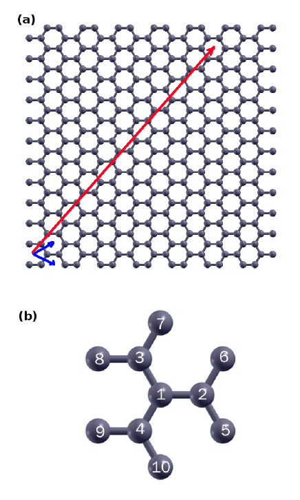
Figure 1: Graphene structure. (a) Honeycomb lattice of graphene. Bases $\vec{a}_{1}$ and $\vec{a}_{2}$ are displayed by two short blue arrows. The long red arrow illustrates a lattice vector $\vec{R}_{-6,15}=-6\vec{a}_{1}+15\vec{a}_{1}$. (b) Sketch of the local environment of atom 1; i.e., three first-nearest and six second-nearest neighboring carbon atoms.

There are two major ingredients in the dynamical matrix. The first one is a phase factor, which is contributed by the space group symmetry of the system. As we known, all unit cells can be repeated by the (0,0) unit cell via a corresponding symmetric operation from the space group. The phase factor, $e^{i\vec{k}\cdot\vec{R}_{l_{1}l_{2}}}$, carries the relationship between the vibration displacement of the (0,0) unit cell and the $(l_{1},l_{2})$ unit cell.

The second ingredient in dynamical matrix is the force constant matrix $K_{00s\alpha;l_{1}l_{2}s^{\prime}\beta}$. The force constant matrix can be obtained mainly through three approaches; i.e., first-principles calculations, empirical potential, or the force constant model. For ionic materials, the shell modelCochran (1959) or the bond charge modelMartin (1969) can be useful for the description of the charge interaction.

In the first two methods, the force constant matrix is calculated by $K_{l_{1}l_{2}s\alpha;l_{1}^{\prime}l_{2}^{\prime}s^{\prime}\beta}=\frac{\partial^{2}V}{\partial u_{l_{1}l_{2}s}^{\alpha}\partial u_{l_{1}^{\prime}l_{2}^{\prime}s^{\prime}}^{\beta}}$, where $V$ is the total potential energy from an empirical potential or the Columb interaction in the first-principles calculations. $u_{l_{1}l_{2}s}^{\alpha}$ is the displacement of the degree of freedom $(l_{1}l_{2}s\alpha)$. This formula is realized numerically by calculating the energy change after displacing a small value for the degrees of freedom $(l_{1}l_{2}s\alpha)$ and $(l^{\prime}_{1}l^{\prime}_{2}s^{\prime}\beta)$. There are some existing packages for such numerical calculation. For instance, some common empirical potentials have been implemented in the lattice dynamic properties package GULP.Gale (1997) It gives the force constant matrix or the phonon dispersion directly. The first-principles package SIESTASoler et al. (2002) also gains some success in the calculation of the force constant matrix or phonon dispersion.

For the third method, there are two popular force constant models for the force constant matrix in graphene, i.e., mass-spring modelJishi et al. (1993) and valence force field model (VFFM).Aizawa et al. (1990) In the mass-spring model, each atom is denoted by a mass, that is connected to other atoms via springs. The force constant of the spring governs the force constant matrix. This model includes two-body interaction. It has been shown that the fourth-nearest neighbors should be included in the calculation of the phonon dispersion of graphene.Saito et al. (1998)

The VFFM aims to capture contribution from the valence electrons on the vibration frequency. Energy variations corresponding to both bond length and bond angle are included in this model. As pointed out by Yu in his book,Yu (2010) a big advantage of the VFFM is its transferability; i.e., force constant parameters in the model are almost the same for the same bonds within different materials. We will illustrate the explicit form of a VFFM for graphene in the following. The VFFM was successful in diamondMusgrave and Pople (1962) and C_dS.Nusimovici and Birman (1967) A simplified version has been proposed by Keating,Keating (1966) which has gained success in many covalent semiconductors.

There are five VFFM terms corresponding to five typical vibration motions for the graphene sheet.Aizawa et al. (1990) The equilibrium position for atom $i$ is $\vec{r}_{i}$. The vector pointing from atoms $i$ to $j$ is $\vec{r}_{ij}=\vec{r}_{j}-\vec{r}_{i}$. The distance between atoms $i$ and $j$ is the modulus $r_{ij}$. We will write out interaction for one bond or one angle explicitly. Fig. 1 (b) illustrates the three first-nearest-neighboring atoms (2-4) and six second-nearest-neighboring atoms (5-10) for atom 1. The interaction for other bonds or other angles can be obtained analogously. The general expressions can be found in Refs. Aizawa et al., 1990; Jiang et al., 2006, 2008.

(1) The bond stretching interaction between atoms 1-2,

$$V_{l}=\frac{k_{l}}{2}[(\vec{u}_{2}-\vec{u}_{1})\cdot\vec{e}_{12}^{~{}l}]^{2}.$$ (7)

$k_{l}$ is the force constant parameter. $\vec{e}_{12}^{~{}l}=\vec{r}_{12}/|\vec{r}_{12}|$ is a unit vector from atom 1 to atom 2. This is the bond stretching interaction between two first-nearest-neighboring atoms. There are similar interactions for other first-nearest-neighboring carbon-carbon bonds, i.e., bond 1-3, 1-4, 2-5, and 2-6.

(2) The bond stretching interaction between atoms 1-5,

$$V_{sl}=\frac{k_{sl}}{2}[(\vec{u}_{5}-\vec{u}_{1})\cdot\vec{e}_{15}^{~{}l}]^{2}$$ (8)

with $k_{sl}$ the corresponding force constant parameter. This term describes the bond stretching interaction between two second-nearest-neighboring atoms. There are similar interactions for other second-nearest-neighboring carbon-carbon bonds.

(3) The angle bending interaction for $\angle 213$ is $V_{BB}$,

$$V_{BB}=\frac{k_{BB}}{2}(\cos\theta^{\prime}_{213}-\cos\theta_{213})^{2};.$$ (9)

where $\theta_{213}$ is the equilibrium angle and $\theta^{\prime}_{213}$ is the angle in vibration. This interaction term describes the bending of angles, which are formed by two first-nearest-neighboring C-C bonds. There are similar interactions for the other angles: $\angle 213$, $\angle 214$, $\angle 314$, $\angle 125$, $\angle 126$, and $\angle 526$.

(4) The out-of-plane bond bending is a four-body interaction. It describes the interaction between atom 1 and its neighboring atoms 2-4. If atom 1 moves out of the plane, then its neighboring atoms 2-4 will try to drag it back to the plane. This potential is, $V_{rc}$,

$$V_{rc}=\frac{k_{rc}}{2}[(3\vec{u}_{1}-(\vec{u}_{2}+\vec{u}_{3}+\vec{u}_{4}))\cdot\vec{e}_{z}]^{2}.$$ (10)

$\vec{e}_{z}$ is the unit vector in the out-of-plane direction. Similar interaction is also applied to atom 2.

(5) If the carbon-carbon bond 1-2 is twisted, then the following twist potential will try to react the twisting motion,

$$V_{tw}=\frac{k_{tw}}{2}[(\vec{u}_{3}-\vec{u}_{4}-(\vec{u}_{6}-\vec{u}_{5}))\cdot\vec{e}_{z}]^{2}.$$ (11)

There are similar twisting interactions for the other first-nearest-neighboring carbon-carbon bonds: 1-3, 1-4, 2-5, and 2-6.

II.3.2 Rigid Translational and Rotational Invariance

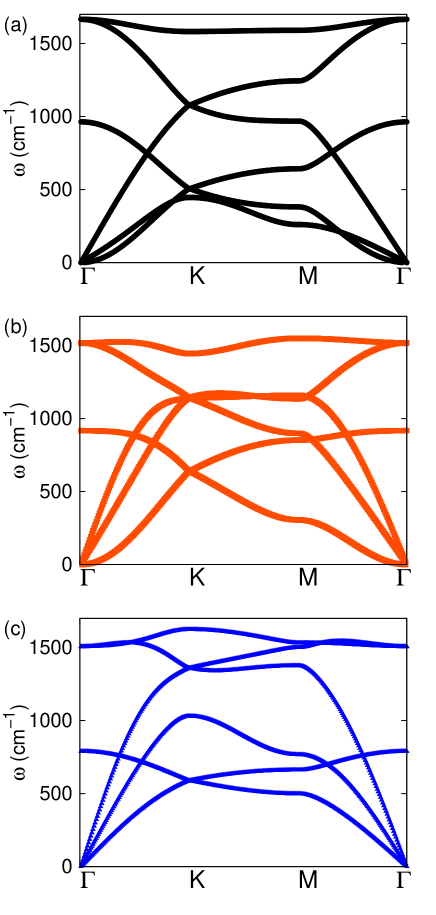
Figure 2: (Color online) The phonon dispersion in graphene along high symmetry lines in the Brillouin zone from (a) Brenner potential, (b) VFFM, and (c) mass spring model.

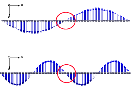
Figure 3: Vibration displacement for two flexural modes in graphene. Arrow on top of each atom represents the vibration component of the atom in this vibration mode. Red circles enclose small pieces of graphene, which are effectively rotated around $y$-axis.

The crystal is rigid in the sense that its total potential energy should not vary if the system is rigidly translated or rotated.Born and Huang (1954) According to this requirement, the empirical potential energy should satisfy two conditions.

• The rigid translational invariance. It says that, if $\vec{u}_{i}=\vec{u}_{0}$ is a constant vector for all atoms, then we should have $\delta V=0$.

• The rigid rotational invariance. It says that, if the system is rotated by $\vec{u}_{i}=\delta\vec{\omega}\times\vec{r}_{i}$, then we should also have $\delta V=0$. Here, the rotation angle is $|\delta\vec{\omega}|$ and the rotation direction is $\frac{\delta\vec{\omega}}{|\delta\vec{\omega}|}$.

We can check that the five terms in the above VFFM satisfy both translational and rotational invariance.

For the translational invariance, the following relationship can be easily found,

$$\vec{u}_{i} = \vec{u}_{j}$$ (12)

$$\vec{u}_{i}-\vec{u}_{j} = 0.$$ (13)

As a result, the translational invariance is satisfied, i.e.,

$$V_{l}=V_{sl}=V_{BB}=V_{rc}=V_{tw}=0.$$ (14)

We will now illustrate the rigid rotational invariance for the above five VFFM potential terms.Jiang et al. (2006) During a rigid rotation motion, the displacement for atom $i$ is

$$\vec{u}_{i}=\delta\vec{\omega}\times\vec{r}_{i}.$$ (15)

As a result, we get following relationship,

$$\vec{u}_{i}-\vec{u}_{j}=\delta\vec{\omega}\times(\vec{r}_{i}-\vec{r}_{j})=\delta\vec{\omega}\times\vec{r}_{ji}.$$ (16)

Using Eq. (16), we can get

$$(\vec{u}_{j}-\vec{u}_{i})\cdot\vec{e}_{ij}^{~{}l}=r_{ij}(\delta\vec{\omega}\times\vec{e}_{ij}^{~{}l})\cdot\vec{e}_{ij}^{~{}l}=0.$$ (17)

As a result, we find that (7) and (8) are zero under a rigid rotational motion, i.e.,

$$V_{l}=V_{sl}=0.$$ (18)

For the the other three potential terms (9), (10) and (11), they become summation over the following expressions, if the system is rotated rigidly,

$$V_{BB} \sim\frac{k_{BB}}{4}[\delta\vec{\omega}\cdot(\vec{e}_{12}^{~{}l}\times\vec{e}_{13}^{~{}l}+\vec{e}_{13}^{~{}l}\times\vec{e}_{12}^{~{}l})]^{2}=0;$$ (19)

$$V_{rc} \sim\frac{k_{rc}}{2}[\delta\vec{\omega}\times(\vec{r}_{12}+\vec{r}_{13}+\vec{r}_{14})\cdot\vec{e}_{1}^{~{}z}]^{2}=0;$$ (20)

$$V_{tw} \sim\frac{k_{tw}}{2}[\delta\vec{\omega}\times(\vec{r}_{43}-\vec{r}_{56})\cdot\vec{e}_{12}^{~{}z}]^{2}=0.$$ (21)

Fig. 2 shows the phonon dispersion in graphene along high symmetric Brillouin line $\Gamma$KM$\Gamma$ using three models. The dispersion in panel (a) is calculated from the Brenner potential.Brenner et al. (2002) In particular, the lowest branch around $\Gamma$ point is the flexural branch with a parabolic spectrum. Panel (b) shows that the spectrum of flexural mode is also parabolic using the VFFM. Parameters in the VFFM are $k_{l}=5.8337$ eVÅ^-2, $k_{sl}=5.2936$ eVÅ^-2, $k_{BB}=10.2245$ eV, $k_{rc}=14.8$ N m^-1, and $k_{tw}=6.24$ N m^-1. However, panel (c) shows that phonon spectrum of the flexural mode from the mass spring model is linear instead of parabolic. It is because the rigid rotation symmetry is violated in the mass spring model. The longitudinal and transverse parameters are considered up to the fourth nearest-neighboring atoms.Jishi et al. (1993) These parameters for the mass spring model are $(k_{l},k_{\perp})=$ (27.7521, 4.4753) eVÅ^-2, (6.8350, 0.1728) eVÅ^-2, (0.5054, 0.1021) eVÅ^-2, and (0.2665, 0.0012) eVÅ^-2. The comparison in Fig. 2 demonstrates that the parabolic spectrum for the flexural mode is closely related to the rigid rotational invariance.

The vibration displacement of the flexural mode is actually directly related to the rigid rotational motion style. Fig. 3 shows the vibration displacement of two flexural modes. The arrow on top of each atom represents the vibration displacement of each atom in this mode. We can divide the system into lots of small pieces along the $x$-axis. It can be shown that each piece is effectively rotated around the y-axis in the flexural mode. Red circles in the figure illustrate two graphene pieces, which are effectively rotated around the y-axis. The rigid rotational invariance leads to zero recovery force for this vibration to first order. That is the micro-origin for the parabolic dispersion of the flexural mode.

For nanotubes with cylindrical hollow structure, the rigid rotational invariance guarantees both the zero frequency of twisting mode and the existence of flexural mode.Mahan and Jeon (2004) The flexural mode (parabolic dispersion) turns into acoustic mode (linear dispersion) gradually with the increase of the thickness of the thin plate. We have used few-layer graphene as an example to show this dimensional crossover phenomenon.Jiang and Wang (2010a)

All three of the phonon spectra in Fig. 2 are computed based on short-range empirical interaction potentials, which are known to be less accurate than first-principles calculations.Dubay and Kresse (2003); Mounet and Marzari (2005); Gillen et al. (2009) This may cause some errors because the long-range interactions may impact the flexural mode. For instance, the long-range dipolar interaction force was considered in a model for the flexural mode in graphene.Metlov (2010) In particular, the crossover in the two in-plane high frequency optical dispersion deviate from the first-principles results.

Although the phonon spectra from empirical potentials less accurate than first principles methods, they have been widely used in practice for many physical phenomena.Al-Jishi and Dresselhaus (1982); Mohr et al. (2007) For instance, classical molecular dynamics simulations are commonly used for the study of the thermal transport in graphene. In principle, the interatomic force can be calculated from first-principles calculations, but the associated computational cost renders such approaches infeasible for systems larger than a thousand or so atoms. Hence, the interatomic force is usually computed from an efficient empirical potentials like the Brenner potentialBrenner et al. (2002) or the Stillinger-Weber potential.Stillinger and Weber (1985) The thermal conductivity obtained from the molecular dynamics simulations can be explained by the phonon spectra of graphene, which should also be calculated based on the same empirical potentials for consistency. In this sense, the phonon spectra that are calculated from empirical potentials are certainly useful, though they are not as accurate as from first-principles calculations.

The inaccuracy in the optical branches in the phonon spectra from empirical potentials will impact some of the computed properties of graphene. For instance, the thermal conductivity of pure graphene is mainly limited by phonon-phonon scattering at room temperature. A typical phonon-phonon scattering process requires the involvement of the optical phonon, so the inaccuracy in the optical branches will lead to some influence on such scattering processes. However, these empirical potentials can give accurate acoustic branches in the phonon spectra, as can be seen from Fig. 2. Acoustic phonon branches are important for many physical phenomena, such as thermal transport. The thermal conductivity in graphene is mainly contributed by its three acoustic phonon branches. As a result, the inaccuracy in the optical branches in the phonon spectra has a much smaller effect on the computed values for the thermal conductivity.

III Thermal Conduction

III.1 Introduction

Thermal transport occurs in the presence of temperature gradient. In metals, both electrons and phonons are important thermal energy carriers to deliver thermal energy. In insulators or semiconductors, phonons carry most of the thermal energy, while electrons only make limited contribution. The thermal conductivity contributed by phonons is called lattice thermal conductivity. Graphene is a well-known semiconductor with zero electronic band gap. Experiments show that the electronic thermal conductivity is aroundYi$\breve{g}$en et al. (2013) 10 W/m$\cdot$K, which is less than 1% of the overall thermal conductivity in graphene.Saito et al. (2007) As a result, the electronic contribution can be safely ignored in the study of the thermal conductivity in graphene. In the following, we focus on the lattice thermal conductivity in graphene.

The thermal conductivity ($\kappa$) and thermal conductance ($\sigma$) are two related concepts that are useful in different thermal transport conditions. They are related to each other from their definitions: $\kappa/L=\sigma/s$, where $L$ and $s$ are the length and the cross-sectional area, respectively. It should be noted that for quasi-two-dimensional materials like graphene, the concept of cross-sectional area is not a well defined concept, because it is only one atom thick. It is crucial to use the same thickness in the comparison of thermal conductivity from different measurements or calculations. The thermal conductance is useful in the ballistic thermal transport regime, which is typically the primary transport mechanism in nanoscale structures. The ballistic transport also happens at very low temperature, where the phonon density is too weak for phonon-phonon scattering. During ballistic transport, each phonon mode delivers a quanta of thermal energy $\hbar\omega$ across the system without scattering. As a result, the thermal conductance is quantized in the ballistic regime.Schwab et al. (2000) The ballistic thermal conductance does not depend on the length of the system, because of the infinite phonon mean free path.

The diffusive thermal transport happens in large systems and/or at high temperatures. The thermal transport ability is mainly limited by phonon related scattering mechanisms in the diffusive regime. In this regime, phonon modes have finite life time and finite mean free path. In other words, the thermal energy carried by a phonon mode get dissipated with increasing distance. In the diffusive regime, the thermal conductivity is a constant with respect to the length of the structure.

The thermal transport in graphene has attracted significant interest after the experimental observation of superior thermal conductivity by Balandin et al. in 2008.Balandin et al. (2008); Ghosh et al. (2008) The quasi-ballistic thermal transport was reported in suspended single-layer graphene below room temperature.Xu et al. (2010) The measured temperature dependence of the thermal conductance scales as $~{}T^{1.5}$, which is consistent with the contribution from the flexural mode to the thermal conductance.Mingo and Broido (2005); Saito et al. (2007); Jiang et al. (2009a) The ballistic thermal conductance in graphene was found to be anisotropic,Jiang et al. (2009a); Xu et al. (2009) while the thermal transport is size-dependent in grapheneMun$\tilde{n}$oz et al. (2010); Wang et al. (2012a); Nika et al. (2012); Xu et al. (2014) following a theoretical two-dimensional disk model.Xiong et al. (2010a) The isotopic doping effect on the thermal conductivity of graphene was investigated theoreticallyJiang et al. (2010a) and verified experimentally,Chen et al. (2012a) and the thermal rectification phenomenon was observed in graphene with asymmetric structures and nonlinear scattering.Yang et al. (2009); Hu et al. (2009); Jiang et al. (2010b, c); Hu et al. (2011); Cheh and Zhao (2012)

Experiments showed that the thermal conductivity in few-layer graphene decreases exponentially with increasing layer number and eventually crosses over to that exhibited by bulk, three-dimensional graphite value.Ghosh et al. (2010) This dimensional crossover phenomenon has received intensive theoretical effort as intrigued by the experimental work by Ghosh et al..Singh et al. (2011); Lindsay et al. (2011); Kong et al. (2009); Zhang and Zhang (2011); Zhong et al. (2011a, b); Rajabpour and Allaei (2012); Cao et al. (2012); Sun et al. (2013); Jiang (2014b) For the single-layer graphene, all of these theoretical works have shown that the single-layer graphene has the highest thermal conductivity among all few-layer graphene systems. For few-layer graphene with layer number above two, most theoretical calculations demonstrated a monotonic decrease of the thermal conductivity with increasing layer number; while the thermal conductivity was found to be independent of the layer number in a recent molecular dynamics simulations.Jiang (2014b)

It is important for nano devices to spread the thermal energy generated during its operation. Graphene has a superior thermal conductivity, which can be very helpful in delivering heat from these devices. For instance, experiments have shown that the graphene based composites have a much higher thermal conductivity owning to graphene’s superior thermal transport ability.Yan et al. (2012); Goyal and Balandin (2012); Shahil and Balandin (2012)

Lots of approaches have been proposed to manipulate the thermal conductivity of graphene, including the application of axial or bending strain,Li et al. (2010); Jiang et al. (2011a); Wei et al. (2011); Gunawardana et al. (2012); Zhang and Wang (2013) edge reconstruction,Jiang et al. (2009b); Lan et al. (2009); Jiang and Wang (2010b); Savin et al. (2010); Tan et al. (2010); Hu et al. (2010) interfaces,Jiang et al. (2011b); Jiang and Wang (2011a); Cheh and Zhao (2011) points defects,Jiang et al. (2011c); Hao et al. (2011); Zhang et al. (2011); Adamyan and Zavalniuk (2012); Serov et al. (2013) wrinkles,Chen et al. (2012b) substrate coupling,Cai et al. (2010); Chen et al. (2011); Lee et al. (2011); Guo et al. (2011); Ong and Pop (2011); Huang et al. (2011); Qiu and Ruan (2012); Guo et al. (2012) and asymmetric interactions,Xiong et al. (2010a); Chen et al. (2012c, 2013a) amongst others.

In the following, we focus on the role of the flexural modes on the thermal conductivity in graphene. There have been a bunch of reviews focusing on different aspects of the thermal conductivity of graphene. Wang et al. discuss the non-equilibrium Green’s function (NEGF) approach in the calculation of the thermal conductivity for nanomaterials.Wang et al. (2008, 2013) The comparison between the thermal conductivity in graphene and other carbon materials was summarized in Ref. Balandin, 2011. Different theoretical approaches to calculating the thermal conductivity in graphene is outlined in Ref. Nika and Balandin, 2012. Several reviews have been devoted to the discussion of the anomalous thermal transport in low dimensional nanoscale systems including graphene.Cahill et al. (2003); Dhar (2008); Liu et al. (2012); Li et al. (2012); Yang et al. (2012a); Luo and Chen (2013); Marconnet et al. (2013) Some basic issues on the heat transport in microscopic level are surveyed in Ref. Dubi and Ventra, 2011 by Dubi and Ventra. Zhang and Li discuss the isotopic doping effect on thermal properties on nanomaterials, including the isotopic doping effect on the thermal conductivity in graphene.Zhang and Li (2010) Heat dissipation in nanoscale electronic device is outlined by Pop in Ref. Pop, 2010.

III.2 Simulation of Thermal Transport

There are several available approaches for the calculation of thermal conductivity. The ballistic thermal conductance can be predicted rigorously by the NEGF approach.Ozpineci and Ciraci (2001); Mingo and Yang (2003); Yamamoto and Watanabe (2006); Wang et al. (2008) For diffusive transport, several approaches are useful, such as the NEGF method,Mingo (2006); Wang et al. (2008) the mode coupling theory,Wang and Li (2004) the Boltzmann transport equation method,Spohn (2006); Lindsay et al. (2011) the classical molecular dynamic (MD) simulation,Lepri et al. (2003) and the quantum non-equilibrium MD simulation.Wang (2007); Wang et al. (2009); Ceriotti et al. (2009a, b); Dammak et al. (2009) The thermal conductivity value can be obtained directly from some open source simulation packages, such as LAMMPS.Lammps (2012) In this section, we illustrate the simulation details for thermal transport using direct MD simulation. The thermal conductivity is determined by the Fourier law.

III.2.1 Fourier’s Law

Fourier’s law is a linear empirical law based on observation. It states that the heat flows from high-temperature region to low-temperature region, and that the thermal current density is proportional to the temperature gradient. We consider the in-plane heat transport along $x$ direction in Fig. 6. In this situation, the Fourier law says,

$$J=-\kappa\frac{dT}{dx},$$ (22)

where $J$ is the thermal current divided by the cross-sectional area and $\kappa$ is the thermal conductivity. The minus sign on the right-hand side indicates that the heat flows from the high-temperature region to the low-temperature region.

It should be noted that the Fourier law is valid only when the local thermal equilibrium is achieved. This linear law requires the thermal conductivity to be a constant with respect to the structure dimension. However, it has been found that the Fourier law is violated in nanomaterials. More explicitly, the thermal conductivity calculated from the Fourier law is size-dependent.Chang et al. (2008); Dubi and Ventra (2009); Yang et al. (2010); Xiong et al. (2010b); Chen et al. (2013b)

According to the Fourier law, the thermal conductivity can be extracted based on the knowledge of the thermal current density and the temperature gradient. In the following, we show how to calculate these two quantities from direct MD simulations.

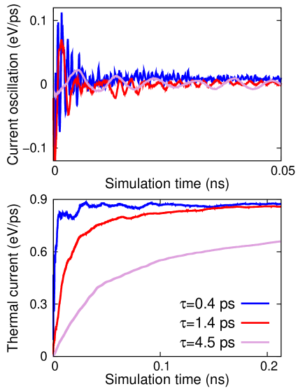
Figure 4: (Color online) The thermal current for different relaxation time ($\tau$) Top: thermal fluctuation. Bottom: the averaged thermal current.

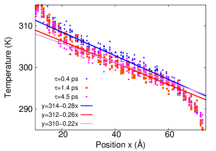
Figure 5: (Color online) Temperature profile. Lines are least squares fits.

III.2.2 Equations of Motion

In the classical direct MD simulation, typically, structure is divided into three regions, i.e., the high temperature-controlled region, low temperature-controlled region, and the free central region. The graphene nanoribbon shown in Fig. 6 has armchair edges. The dimension is $185\times 12.3$ Å. The thickness of the graphene is taken to be 3.35 Å. This is the inter-layer distance in the three-dimensional graphite.Saito et al. (1998) The fixed boundary is applied in the x-direction, i.e., both left and right ends are fixed during the simulation. Periodic boundary condition is applied in the y-direction. Free boundary is applied in the out-of-plane direction.

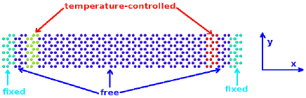
Figure 6: (Color online) The graphene is divided into three different regions, including the two fixed ends, the two temperature-controlled regions, and the free region.

In the central region, the degrees of freedom for atom $i$ ($\vec{r}_{i}$, $\vec{v}_{i}$) are controlled by the following equation of motion,

$$\frac{d\vec{r}_{i}}{dt} = \vec{v}_{i},$$ (23)

$$\frac{d\vec{v}_{i}}{dt} = -\frac{1}{m_{i}}\frac{\partial V}{\partial\vec{r}_{i}}.$$ (24)

The Brenner potential is used to describe the interatomic interaction in this calculation.Brenner et al. (2002) The time evolution for each atom can be obtained by solving Eq. (24) numerically.

In the temperature-controlled regions, the motion of the atom is influenced by the heat bath besides the inter-atomic force. The heat bath helps to keep a constant temperature for these regions. The heat bath is described by the thermostat degrees of freedom. There are various thermostat algorithms for temperature controlling, such as Nóse-Hoover heat bath,Nose (1984); Hoover (1985) the classical or quantum Langevin heat bath,Wang (2007); Wang et al. (2009); Ceriotti et al. (2009a, b); Dammak et al. (2009) amongst others. We take the Nóse-Hoover heat bath as an example in the following demonstration of the simulation for the thermal transport. The movements of these atoms in the temperature-controlled regions are governed by the following coupled dynamic equations,

$$\frac{d\vec{r}_{i}}{dt} = \vec{v}_{i},$$ (25)

$$\frac{d\vec{v}_{i}}{dt} = -\frac{1}{m_{i}}\frac{\partial V}{\partial\vec{r}_{i}}-\eta_{i}\vec{v}_{i},$$ (26)

$$\frac{d\eta_{i}}{dt} = \left(\sum_{j}m_{j}v_{j}^{2}-gk_{B}T\right)/Q.$$ (27)

$$Q = gk_{B}T\tau^{2},$$ (28)

$g$ is the total degrees of freedom in the temperature-controlled region. $\tau$ represents the interaction strength between the heat bath and the system, so it is a kind of thermal relaxation time for the Nóse-Hoover heat bath. This thermal relaxation time has some direct effect on the thermal current across the system as shown in Fig. 4. The top panel is for the thermal fluctuation and the bottom panel is the average thermal current. For $\tau=4.5$ ps, the response from the heat bath is very slow, so it corresponds to a weak coupling between the heat bath and the system. In this case, a longer thermalization time is needed to realize a stable temperature distribution across the system, although the influence from the heat bath is smaller. For $\tau=0.4$ ps, the heat bath can respond very fast, so the heat bath couples with the system strongly. As a result, shorter thermalization time is required, but the heat bath will induce more influence to the system. Similar thermal current are obtained for $\tau=0.4$ ps and 1.4 ps. Simulations with different relaxation time result in almost the same thermal conductivity.

III.2.3 Thermal Current and Temperature Gradient

The fundamental effect of the heat baths is to inject thermal energy into the system through the high-temperature region, and pump out the same amount of thermal energy in the low-temperature region. Due to energy conservation, the thermal current across the system should equal to the energy exchange between the heat bath and system in the temperature-controlled regions, as long as there is no energy accumulation in the system.Poetzsch and B$\ddot{o}$ttger (1994); Jiang et al. (2010a)

From Eq. (28), it can be found that,

$$m_{i}v_{i}\frac{dv_{i}}{dt} = -v_{i}\frac{\partial V}{\partial r_{i}}-\eta_{i}m_{i}v_{i}^{2},$$ (29)

so we have the following equation,

$$\frac{d}{dt}\left(\sum_{i}\frac{1}{2}m_{i}v_{i}^{2}\right)+\frac{dV}{dt} = -\sum_{i}\eta_{i}m_{i}v_{i}^{2}.$$ (30)

The left-hand side is the rate of change in the total energy. As a result, we get the energy flowing from the heat bath to the system,

$$E_{ex} = -\int_{t_{0}}^{t_{0}+\Delta t}\sum_{i}\eta_{i}m_{i}v_{i}^{2}dt.$$ (31)

$\Delta t$ is the total simulation time. The summation index $i$ runs over all atoms in the temperature-controlled region. We can thus compute the thermal current in a more symmetric manner,

$$J=\frac{1}{s}\frac{E_{ex}^{high}-E_{ex}^{low}}{2\Delta t},$$ (32)

with $s$ as the cross-sectional area. $E_{ex}^{high}$ and $E_{ex}^{low}$ are energy from heat bath on the left and right sides. The thermal current is shown in Fig. 4. The thermal fluctuation is $dJ=\frac{E_{ex}^{high}-E_{ex}^{low}}{2\Delta t}$. The cross-sectional area is not included for these data shown in the figure. For $\tau=$ 0.4, 1.4, and 4.5 ps, the thermal currents are 0.87, 0.86, and 0.66 eV/ps, respectively.

Eqs. (24) and (28) are solved iteratively, by discretizing the time with a small time step, where the time step in MD simulations for graphene is usually on the order of femtoseconds. The highest-frequency phonon mode in graphene is the in-plane optical mode, with frequency around 300 THz. For a time step of 1.0 fs, there are about 20 simulation steps within one oscillation cycle of the optical mode. The trajectory of each atom and the thermostat parameter from the iterative solution are used to compute the thermal current.

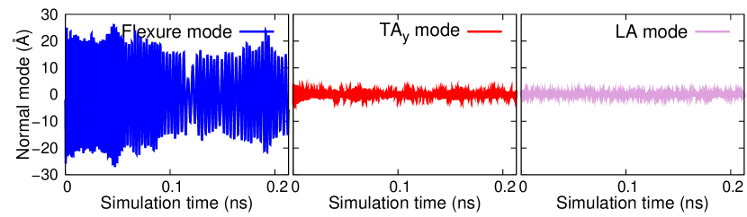
Figure 7: (Color online) Normal mode coordinate extracted from MD simulation at room temperature for the first flexural mode (left), the first in-plane transverse acoustic mode (center), and the first longitudinal acoustic mode (right).

The average kinetic energy for each atom gives the temperature for the atom according to the equipartition theorem $\frac{1}{2}(v_{x}^{2}+v_{y}^{2}+v_{z}^{2})=\frac{3}{2}k_{B}T$, where $k_{B}$ is the Boltzmann constant. Hence, the temperature profile $T(\vec{r}_{i})$ is obtained simultaneously from the MD simulation. Fig. 5 shows a typical temperature profile in graphene. The temperature profile within the central region $x\in[0.25L,0.75L]$ is linearly fitted to give the temperature gradient within the system. The resulted temperature gradients are -0.28, -0.26, and -0.22 K/Å, for the three different relaxation times $\tau=$ 0.4, 1.4, and 4.5 ps. The thermal conductivity can then be extracted through the Fourier law in Eq. (22). The obtained thermal conductivity values are 120.9, 128.7, and 116.7 W/m$\cdot$K.

III.3 Contribution from Flexural Mode

III.3.1 Long Lifetime for Flexural Mode

It was shown in several recent works that the Fourier law is not valid in nanoscale structures,Cahill et al. (2003); Dhar (2008); Liu et al. (2012); Xu et al. (2014) where the thermal conductivity becomes size-dependent and increases with increasing length. For quasi-one-dimensional nanostructures, the thermal conductivity can be written as a power function of the length, i.e., $\kappa\propto L^{\beta}$, where the exponent $\beta=0$ for purely diffusive transport and $\beta=1$ for purely ballistic transport. The exponent deviates from 0, and becomes size-dependent in nanomaterials; i.e., the Fourier law is violated.

The contribution from each phonon mode to the thermal conductivity can be collected as follows,Hone et al. (1999); Gu and Chen (2007); Jiang and Wang (2011b)

$$\kappa_{\rm ph}=\frac{1}{V}\sum_{\vec{k}}\tau_{\vec{k}}^{\sigma}C_{\rm ph}(\omega)v_{\vec{k}}^{2}.$$ (33)

$V$ is the volume of the system. $C_{\rm ph}=k_{B}x^{2}e^{x}/(e^{x}-1)^{2}$ is the heat capacity. $x=\hbar\omega/(k_{B}T)$. $v_{\vec{k}}$ is phonon group velocity in the thermal flow direction. The lifetime for each phonon in this formula can be obtained using the single mode relaxation time approximation. Following formula gives the the lifetime for phonon mode $\vec{k}$ due to phonon-phonon scattering,

$$\frac{1}{\tau_{\rm ps}} = \left(\frac{4}{3\rho_{L}}\right)\left(\frac{\hbar\omega\gamma^{2}}{v_{z}^{2}}\right)\sum_{n^{\prime}\sigma^{\prime}}^{\prime}\frac{1}{v_{g}}\omega^{\prime}\omega^{\prime\prime}N\left(\omega^{\prime},\omega^{\prime\prime}\right).$$ (34)

In this formula, $\rho_{L}$ is the mass per length. $v_{z}$ is the phonon velocity along the thermal current direction. $v_{g}=|v^{\prime}-v^{\prime\prime}|$ is the group velocity. The energy and momentum conservation is implicated by the prime over the summation.

The phonon-phonon scattering is weak at low temperature, so the boundary scattering becomes more important, especially for systems with small size. Hence, it is also important to consider the boundary scattering process,Ziman (1960)

$$\frac{1}{\tau_{\rm bs}} = \frac{v_{\vec{k}}^{\sigma}}{L}\times\frac{1-p}{1+p},$$ (35)

where $p$ is the spectacular parameter. The overall phonon lifetime can be obtained as,

$$\frac{1}{\tau_{\rm tot}} = \frac{1}{\tau_{\rm ps}}+\frac{1}{\tau_{\rm bs}}.$$ (36)

The above formula gives the phonon lifetime and thermal conductivity due to boundary scattering and phonon-phonon scattering. It was found that, in the frequency range [50, 80] cm^-1, the lifetime for the flexural mode is dominated by the boundary scattering, as the phonon-phonon scattering is weak.Jiang and Wang (2011b) These phonons with long lifetime transport across the system almost ballistically, while the other phonons with short lifetime behavior diffusively. As a result, the overall behavior for the thermal conductivity is sandwiched between the ballistic and diffusive transport regimes, i.e., the power factor $\beta$ sits in $[0,1]$.

The thermal conductivity in graphene was found to increase with increasing size even in the $\mu$m range.Nika et al. (2009a, b) When the width of the graphene is enlarged by a factor of 3, the thermal conductivity increases by about a factor of 1.8. There is still no conventionally accepted argument for such violation of the Fourier law in graphene.

It is clear that the three acoustic phonon branches make the largest contribution to the the thermal conductivity for graphene. However, there is still no universally accepted fact on the relative contribution from the flexural mode to the thermal conductivity in graphene. Typically, the contribution from the flexural mode depends on the temperature or defect density or the substrate for the graphene sample. For perfect graphene, using Boltzmann transport theory, Lindsay et al. found that the flexural mode dominates the thermal conductivity of the graphene.Lindsay et al. (2011) The flexural mode contributes about 70% of the thermal conductivity in graphene, while each of the other two acoustic phonon modes contribute 10%. The large contribution from the flexural mode is attributed to the large density of states of the flexural mode, and the strict symmetry selection rule imposed on the flexural mode, which leads to very long lifetime of the flexural mode. We note that the symmetry selection rules are demonstrated in the first Brillouin zone, which was combined with the phonon-phonon scattering formula Eq. (34) to give the extremely long lifetime for the flexural mode in graphene.Nika et al. (2009a)

In other works, the flexural mode has been found to make a smaller contribution than the other two acoustic (LA and in-plane TA) modes, especially at higher temperature.Nika et al. (2009a); Aksamija and Knezevic (2011); Nika and Balandin (2012); Chen and Kumar (2012) Aksamijaa and Knezevicb found that the flexural mode has about a 50% contribution at temperatures bellow 130 K for graphene with rough edges.Aksamija and Knezevic (2011) However, the flexural mode contribution decreases quickly with increasing temperature, and the contribution from the flexural mode becomes less than 20% at 400 K. Chen and Kumar found that the LA mode dominates the thermal conductivity of both isolated and supported graphene on Cu substrate.Chen and Kumar (2012)

Furthermore, in practice, the symmetry selection rule will be relaxed in experiments, where the high symmetry of the perfect graphene is broken. For instance, the symmetry will be lowered in suspended graphene samples, which is inevitably bent during measurement. In this situation, the lifetime of the flexural mode should be considerably reduced. For deformed graphene samples, it is difficult to use the Boltzmann transport theory to compute the thermal conductivity, because the symmetry selection rule no longer valid. Therefore, classical MD simulations can be used to study the thermal transport in the deformed graphene or graphene with defects.

Several theoretical works have shown that the temperature dependence will scale as $~{}T^{1.5}$ at low temperature for the thermal conductance contributed by the flexural mode in the ballistic regime.Mingo and Broido (2005); Saito et al. (2007); Jiang et al. (2009a) In a recent experiment, Xu et al. measured the thermal conductivity of the graphene in a quasi-ballistic regime and found that the temperature dependence of the thermal conductivity scales asXu et al. (2010) $~{}T^{1.5}$, which is the same as the theoretical predictions. This consistency gives one piece of evidence that the flexural mode makes an important contribution to the thermal transport in graphene in the quasi-ballistic regime. However, it should be noted that, in practice, the sample quality plays an important role on the temperature-dependence of the thermal conductivity. In particular, the temperature-dependence for the thermal conductivity in graphene is sensitive to the defect densities or the grain size of the graphene sample.Adamyan and Zavalniuk (2012); Serov et al. (2013)

III.3.2 Projection Operator for Flexural Mode

We provide a normal mode projection operator for analyzing the contribution from the flexural mode to the thermal conductivity in MD simulations. From the lattice dynamic properties of the flexural mode discussed in Sec.II, we can determine the eigenvector for the flexural mode. The position of atom $i$ is determined by the vector $\vec{r}_{i}$. The eigenvectors can be used to define the normal mode projection operator, $P^{k}$,

$$P^{k}=(\vec{\xi}_{1},\vec{\xi}_{2},\vec{\xi}_{3},...,\vec{\xi}_{N})$$ (37)

where $N$ is the total number of atoms. From MD simulations, we have the time history of the vibration displacement of each atom,

$$\vec{u}_{i}(t)=\vec{r}_{i}(t)-\vec{r}_{i}^{0}.$$ (38)

where $\vec{r}_{i}^{0}$ is the initial position for atom $i$. Applying the normal mode projection operator, $P^{k}$, onto the vibration displacement vector will give us a scalar normal mode coordinate, $Q^{k}(t)$,

$$Q^{k}(t)=\sum_{i=1}^{N}\vec{\xi}_{i}^{*}\cdot\vec{u}_{i}(t).$$ (39)

The normal mode projection technique can selectively disclose the contribution to the thermal conductivity from each phonon mode. Fig. 7 compares the normal mode coordinate of the first flexural mode, in-plane transverse acoustic mode, and longitudinal acoustic mode from the MD simulation at 300 K. It is clear that the flexural mode has much larger normal mode amplitude than the other two modes, indicating that the flexural mode is the most important vibration morphology in the graphene during the MD simulation. It shows explicitly that the major contribution is from the flexural mode to the thermal conductivity.

III.3.3 Tuning the Thermal Conductivity Via Flexural Mode

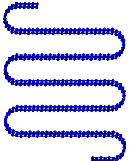
Figure 8: (Color online) Graphene is folded, introducing the inter-layer coupling for the flexural mode.

The graphene is very flexurable in the out-of-plane direction, so it is easier to modify the flexural mode. Hence, it will be an efficient way to manipulate the thermal conductivity through the flexural motion.

The first method is to introduce inter-layer coupling for the flexural mode; e.g., coupling different graphene monolayers to form a few-layer graphene. Indeed, it was observed in experiment that the thermal conductivity is considerably reduced by increasing layer numbers in few-layer graphene.Ghosh et al. (2010) The thermal conductivity in bilayer graphene is about 30% lower than that of the single-layer graphene. The reduction of the thermal conductivity is attributed to the enhanced phonon-phonon scattering for the flexural mode in thicker few-layer graphene, where more scattering channels are available.

The second direct method to manipulate the flexural mode is to fold the graphene as shown in Fig. 8. A fold will introduce inter-layer coupling to the flexural mode.Ouyang et al. (2011); Yang et al. (2012b) This coupling can be further increased by compression the inter-layer space in the folds. For a flat graphene, flexural mode is difficult to scatter with phonon modes from the high-frequency optical branches, because the band gap between the flexural mode and the optical branches is very large due to the parabolic spectrum of the flexural mode. However, the phonon-phonon scattering channels are considerably increased when the inter-layer space is compressed in the folds. The compression of the inter-layer space leads to considerable shifting up of the flexural phonon spectrum, thus narrowing the band gap between the flexural mode and the optical branches. As a result, the phonon-phonon scattering channels increase significantly. This results in a reduced thermal conductivity in folded graphene.

The third method to manipulate the flexural mode is to put the graphene on a substrate.Cai et al. (2010); Chen et al. (2011); Lee et al. (2011); Guo et al. (2011); Ong and Pop (2011); Huang et al. (2011); Qiu and Ruan (2012); Guo et al. (2012) The thermal conductivity can be reduced by an order of magnitude due to damping of the flexural mode by the substrate.Ong and Pop (2011) Furthermore, the increase in the coupling strength between graphene and substrate will enhance the thermal conductivity. It is because of the coupling of the flexural mode to the substrate Rayleigh waves, which results in a hybridized mode with linear spectrum and higher group velocity than the original flexural mode in graphene. Quite recently, Amorim and Guinea examined the flexural mode of graphene on different substrates, with the consideration of the dynamics of the substrate.Amorim and Guinea (2013)

IV Thermal Expansion

IV.1 Introduction

Negative coefficient of thermal expansion (CTE) occurs in many materials, typically at low temperature. For example, bulk Si and Ge are two well-known semiconductors with negative CTE at temperatures below 100 K, which is attributed to the inter-play between the bond-stretching and bond-bending forces.Xu et al. (1991); Wei et al. (1994) Ref. Barrera et al., 2005 summarizes the negative CTE in different materials and various possible mechanisms underlying this phenomenon.

The CTE for graphene was also found to be negative. On the experimental side, in 2009, the CTE is found to be about $-7\times 10^{-6}$ K^-1 at room temperature as measured by Bao et al.Bao et al. (2009) The room temperature CTE is about $-8\times 10^{-6}$ K^-1 in the experiment by Yoon et al..Yoon et al. (2011) The measured CTE is negative in a wide temperature range. Singh et al. found that graphene has a negative CTE for temperatures bellow 300 K,Singh et al. (2010) while Yoon et al. obtained a negative CTE for graphene for temperatures bellow 400 K.Yoon et al. (2011)

On the theoretical side, there are several standard approaches to compute the CTE. The lattice constant is temperature dependent, which can be used to extract the CTE value.Mounet and Marzari (2005); Zakharchenko et al. (2009); Pozzo et al. (2011) These calculations show a minimum lattice constant at a transition temperature. Below this transition temperature, the CTE decreases with increasing temperature. Above this transition temperature, the CTE increases with increasing temperature. This implies that CTE is negative below the transition temperature and becomes positive above the transition temperature. In our recent work, the NEGF approach was implemented to compute the CTE of graphene.Jiang et al. (2009c) As an advantage of the NEGF approach, this method is able to account for the quantum zero-point vibration effect in a quite natural manner. Another advantage of the NEGF approach is that it is straightforward to decompose the contribution of each phonon mode to the total CTE value. We will mainly discuss this NEGF approach in the following.

IV.2 Green’s Function Approach for Thermal Expansion

The thermal expansion is usually studied by MD simulations or the standard Grüneisen method.Gruneisen (1926) In our recent work, the NEGF approach is used to examine the thermal expansion phenomenon in the single-walled carbon nanotube and graphene, where the calculated CTE agrees quite well with experiments.Jiang et al. (2009c) In this section, we review some key steps in this NEGF approach for the thermal expansion.

IV.2.1 Green’s Function Approach

The potential energy associated with the phonon modes are assumed to be,

$$V = \sum_{ij}\frac{K_{ij}}{2}u_{i}u_{j}+H_{n}.$$ (40)

It includes linear and nonlinear interactions. Both third and fourth orders nonlinear interactions are considered,

$$H_{n}=\sum_{lmn}\frac{k_{lmn}}{3}u_{l}u_{m}u_{n}+\sum_{opqr}\frac{k_{opqr}}{4}u_{o}u_{p}u_{q}u_{r}.$$ (41)

$K_{lmn}$ and $K_{opqr}$ are force constant matrix elements. We have extracted the nonlinear coefficients $k_{lmn}$ and $k_{opqr}$ from the Brenner potential.Brenner et al. (2002)

Details for the Green’s function approach in thermal properties can be found in Refs. Wang et al., 2008, 2013. We utilize the following two GFs for the study of the thermal expansion,

$$G_{j}(\tau) = -\frac{i}{\hbar}\langle T_{\tau}u_{j}^{H}(\tau)\rangle,$$ (42)

$$G_{jk}(\tau,\tau^{\prime}) = -\frac{i}{\hbar}\langle T_{\tau}u_{j}^{H}(\tau)u_{k}^{H}(\tau^{\prime})\rangle.$$ (43)

$u_{j}^{H}(\tau)$ is the vibrational displacement. For convenience, $u_{j}^{H}(\tau)$ also includes the square root of the atom’s mass. It is very nice that $G_{j}$ can be obtained analytically,

$$G_{j}=\sum_{lmn}k_{lmn}G_{lm}^{>}(0)\tilde{G}_{nj}^{r}[0].$$ (44)

$G^{>}(0)$ is the greater GF in time domain. $\tilde{G}^{r}[0]$ is the retarded GF in frequency domain. These two GFs can be computed without any integration. Using Eq. (42), we get the average vibrational displacement for atom $j$, i.e., $\langle u_{j}\rangle$. CTE can be computed from the derivative of the displacement with respect to the temperature.

It is more convenience to work in the normal mode space for the derivative of the one-point GF. After the Fourier transformation, we get,

$$\frac{dG_{j}}{dT} = (-i)\sum_{lmn}k_{lmn}\left(S\left(\begin{array}[]{ccc}\ddots\\ &\frac{1}{\omega_{\mu}}(\frac{df}{dT})\\ &&\ddots\end{array}\right)S^{\dagger}\right)_{lm}$$ (47)

$$\times\left(-K^{-1}\right)_{nj},$$

where $f$ is the Bose distribution function. $K$ is the force constant matrix. $S$ stores the eigen vector of $K$, i.e., $S^{\dagger}KS$ is diagonal with diagonal elements $\omega^{2}_{\mu}$.

A particular boundary condition is used for the NEGF treatment of the thermal expansion phenomenon. Specifically, the left end is fixed, while the right end is free. Periodic boundary condition is applied in the in-plane lateral direction. It was shown that graphene has a negative CTE for temperatures bellow 600 K.Jiang et al. (2009c) The minimum CTE value is achieved around 200 K. These results are in good agreement with the experimental findings. The NEGF approach is able to examine the substrate coupling effect, which has been found to be important for the CTE value of graphene.Pozzo et al. (2011)

IV.2.2 Green’s Function Approach and Grüneisen Method

We will show that the NEGF approach is equivalent to the traditional Grüneisen method in the weak nonlinear limit, if the system is isotropically and uniformly deformed in the thermal expansion phenomenon.Wang and Jiang (2014)

From above, the CTE from NEGF for atom $N$ is,

$$\alpha_{N} = \frac{1}{L}\sum_{lmn\mu}k_{lmn}S_{l\mu}S^{*}_{m\mu}\frac{c_{\mu}}{\omega_{\mu}^{2}}\left(-K_{nN}^{-1}\right),$$ (48)

where $c_{\mu}=\hbar\omega_{\mu}df/dT=C_{rmph}(\omega_{\mu})$ is the heat capacity for phonon mode $\mu$ as introduced in Eq. (33). The Grüneisen parameter for mode $\mu$ is,

$$\gamma_{\mu} = -\frac{\partial\ln\omega_{\mu}}{\partial\ln V}$$ (49)

$$= -\frac{L}{3\omega_{\mu}^{2}}\sum_{lmn}S_{l\mu}S^{*}_{m\mu}k_{lmn}\epsilon_{n},$$

where $\epsilon_{n}=\delta R_{n}/L$ is the change of position for atom $n$ with respective to total length $L$. The CTE from Grüneisen method is then,

$$\alpha = \frac{1}{3B}\left(\frac{\partial P}{\partial T}\right)_{V}$$ (50)

$$= \frac{1}{3BV}\sum_{\mu}\gamma_{\mu}c_{\mu}$$

$$= -\frac{1}{B}\sum_{lmn\mu}\epsilon_{n}k_{lmn}S_{l\mu}S^{*}_{m\mu}\frac{c_{\mu}}{\omega_{\mu}^{2}},$$

where $P$ is pressure, $B$ is bulk modulus, $V$ is volume, and an isotropic and uniform deformation has been assumed for the system during the thermal expansion phenomenon.

To show the equivalence between these two methods, let’s assume the system undergoes a uniform deformation by external force $F$. In this situation, the displacement of atom $n$ can be obtained from the force constant matrix, or equivalently from the bulk modulus,

$$u_{n} = K_{nN}^{-1}F=\epsilon_{n}\frac{FL}{B},$$ (51)

so,

$$\frac{1}{B}\epsilon_{n} = \frac{K_{nN}^{-1}}{L}.$$ (52)

As a result, we find that,

$$\alpha = \alpha_{N}.$$

From the comparison, we show that the NEGF approach has three advanced properties over the Grüneisen method. First, the NEGF approach can be applied to study structures which have a nonuniform deformation, while the Grüneisen method can only be applied for structures with uniform deformation in the thermal expansion phenomenon. Second, the NEGF approach is applicable for nanostructures without periodicity, while the Grüneisen method requires periodicity with a well-defined bulk modulus. Third, the NEGF approach is suitable for systems with anisotropic CTE, while Grüneisen method only works for systems with isotropic CTE.

In the meantime, we point out two disadvantages for the NEGF approach as compared with the Grüneisen method. First, the calculation of $K^{-1}$ is computationally expensive in the NEGF approach, especially for large systems. Hence, in terms of computation cost, the Grüneisen method is better than the NEGF approach for materials with isotropic CTE, where both methods are applicable. Second, the NEGF approach is based on a perturbation theorem and high-order nonlinear terms have been omitted; while Grüneisen method includes an overall effect from all high-order nonlinear interaction terms.

IV.3 Contribution from Flexural Mode

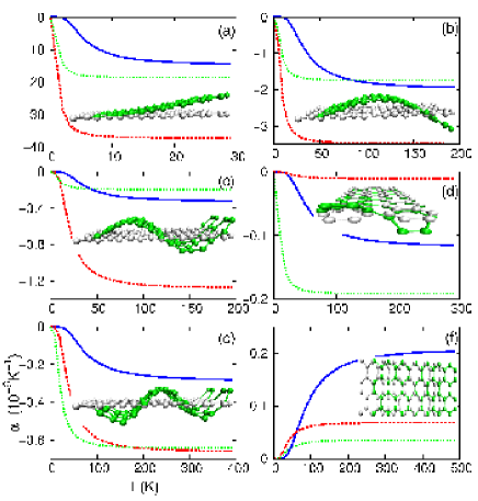
Figure 9: Contribution to CTE from six lowest-frequency phonon modes in graphene sheet without substrate interaction. Blue solid line is for graphene with (length, width)=(10, 8.5) Å, green dashed line is for (20, 17) Å and red dotted line is for (20, 8.5) Å. Insets are the vibrational morphology for the corresponding mode. (a), (b), (c) and (e) are the first four bending modes. (d) is a tearing mode. (f) is the longitudinal phonon mode.

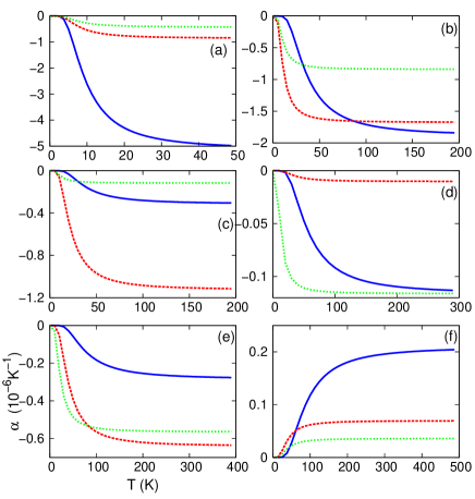
Figure 10: Contribution to CTE from six lowest-frequency phonon modes in graphene sheet with substrate interaction $\gamma=0.001$.

We will now demonstrate that the large negative CTE in graphene is due to its flexural modes. Eq. (47) includes the contribution from all phonon modes to the CTE through the diagonal matrix,

$$\left(\begin{array}[]{ccc}\ddots\\ &\frac{1}{\omega_{\mu}}(\frac{df}{dT})\\ &&\ddots\end{array}\right).$$ (54)

This matrix is diagonal, which indicates that each phonon mode makes separate contributes for the negative CTE. If this matrix has a single nonzero element, $\frac{1}{\omega_{\mu}}(\frac{df}{dT})$, then Eq. (47) yields the sole contribution from the mode $\mu$. Hence, we can distinguish the independent contribution from each phonon mode to the CTE.

Fig. 9 shows the contribution from the six lowest-frequency phonon modes. There is no substrate interaction in this figure, i.e., $\gamma=0$. The inset in each panel is the corresponding vibration morphology of the phonon mode. (a), (b), (c) and (e) are the first four bending modes and (d) is an interesting tearing mode. Among all of these six phonon modes, the first bending mode shown in (a) has $90\%$ contribution to CTE. Due to its bending morphology, this mode induces a contraction effect in the graphene sheet, and thus the negative CTE.

If the substrate interaction is nonzero as shown in Fig. 10, the CTE is clearly enhanced and the size effect becomes weaker. The contribution from the second bending mode is also very important. The substrate interaction is more important for larger piece of graphene, because the bending movement in larger graphene is more serious than smaller piece of graphene when it is fixed on one edge. In case of strong substrate interaction, graphene is so difficult to be bent that all bending modes do not contribute. In this situation, the CTE is dominated by the sixth mode, which leads to a positive CTE. As a result, the CTE is positive in whole temperature range, and the size effect on the CTE becomes smaller.

V Young’s Modulus

V.1 Introduction

Graphene has many remarkable mechanical properties. Readers are referred to Refs. Li et al., 2009; Terrones et al., 2010; Yang et al., 2012c; Lau et al., 2012; Tu and Ou-Yang, 2008 for comprehensive reviews on various mechanical properties of graphene. For instance, the Young’s modulus for graphene is on the order of TPa. There are several different approaches for the investigation of the Young’s modulus. The atomic force microscope can measure the force-displacement relationship for graphene, from which the Young’s modulus can be extracted. This method is used in the experiment in 2008, which found the Young’s modulus for graphene to be $1.0\pm 0.1$ TPa. This method has also been adopted in some theoretical works to study the Young’s modulus in graphene.Lu (1997); Lier et al. (2000); Kudin et al. (2001); Konstantinova et al. (2006); Reddy et al. (2006); Huang et al. (2006); Liu et al. (2007); Khare et al. (2007); Wei et al. (2009); Jiang et al. (2010d); Yi and Chang (2012); Zhou et al. (2013)

The classical theory of elasticity has been widely used to predict the mechanical properties for graphene. Finite element simulations, which are based on a numerical discretization of the equations of elasticity, were used to explain the edge stress induced warping phenomenon in the graphene nanoribbon.Shenoy et al. (2008) The finite element method has also been coupled with atomistic calculations to simulate the crack propagation in graphene in an efficient way.Khare et al. (2007) The elasticity approach has also been combined with atomic potentials to study elastic properties for finite size graphene.Reddy et al. (2006); Duan and Wang (2009)

As an ultra-thin plate, graphene’s flexural mode is directly related to its Young’s modulus.Landau and Lifshitz (1995) The flexural mode has the lowest frequency, so this mode is the easiest to be excited by thermal vibration. As a result, the thermal vibration of graphene is closely related to its Young’s modulus. Using this relationship, it is possible to extract the Young’s modulus from the thermal vibrations. In 1996, this idea was implemented by Treacy et al. to measure the Young’s modulus of carbon nanotubes.Treacy et al. (1996); Krishnan et al. (1998) In our recent work, we applied this method to compute the Young’s modulus from graphene’s thermal vibration.Jiang et al. (2009d) In this section, we will review this approach and emphasize the relationship between the flexural mode and the Young’s modulus of graphene.

V.2 Flexural Mode and Young’s Modulus

In the elasticity theory, the flexural mode is directly related to the Young’s modulus of a plate. Here we review some key derivation steps for the Young’s modulus of graphene.Jiang et al. (2009d) The flexure mode for the elastic plate is governed by the following equation,Landau and Lifshitz (1995)

$$\rho\frac{\partial^{2}z}{\partial t^{2}}+\frac{D}{h}\Delta^{2}z=0,$$ (55)

where $\rho$ is the mass density. $D=\frac{1}{12}Yh^{3}/(1-\mu^{2})$ is the bending modulus. $Y$ is the Young’s moduls. $\mu$ is the Poisson ratio. $h$ is the thickness of the plate. This partial differential equation can be solved after the following boundary conditions are applied,

$$z(t,x=0,y) = 0,$$

$$z(t,x=L,y) = 0,$$ (56)

$$z(t,x,y+L) = z(t,x,y).$$

According to this boundary condition, we can get following solution,Polyanin (2002)

$$\omega_{n} = k_{n}^{2}\sqrt{\frac{Yh^{2}}{12\rho(1-\mu^{2})}},$$

$$z_{n}(t,x,y) = u_{n}\sin(k_{1}x)\cdot\cos(k_{2}y)\cdot\cos(\omega_{n}t),$$ (57)

$$\vec{k} = k_{1}\vec{e}_{x}+k_{2}\vec{e}_{y}.$$

The two wave vector components are $k_{1}=\pi n_{1}/L$ and $k_{2}=2\pi n_{2}/L$. This flexural mode is characteristic for its parabolic phonon dispersion in the long wave limit. This solution shows explicitly the relationship between the frequency of the flexural mode and the Young’s modulus.

At finite temperature, the thermal vibration of the plate is mainly controlled by the lowest-frequency flexural mode. The Young’s modulus can be related to the thermal mean square vibration amplitude $\langle\sigma^{2}\rangle$ as follows,

$$Y = 0.3\times\frac{S}{h^{3}}\times\frac{k_{B}T}{\langle\sigma^{2}\rangle}.$$ (58)

The thickness is chosen as $h=3.35$ Å. The Poisson ratio for graphene is $\mu=0.17$.Blakslee et al. (1970); Portal et al. (1999) $S$ is the area. Eq. (58) can be used to extract the value for the Young’s modulus of graphene. MD simulations are performed to obtain the thermal vibration quantity $\langle\sigma^{2}\rangle$.

Eq. (58) is derived based on the elasticity theory shown in Eq. (55). In principle, the elastic theory works only for very large system. However, it has been shown that the elastic continuum theory is still valid in a very small piece of graphene.Kudin et al. (2001) Such elasticity theory has also been successfully applied to compute the elastic ripple-like deformation at free edges in finite graphene nanoribbons and other mechanics properties.Reddy et al. (2006); Shenoy et al. (2008); Reddy et al. (2009); Wei et al. (2009); Cadelano et al. (2009)

From the above, we are aware that the flexural mode, especially the first flexural mode, is closely related to the Young’s modulus of graphene. More specifically, the frequency of the flexural mode is proportional to the square root of the Young’s modulus. The flexural mode describes the out-of-plane bending movement of graphene. However, it is quite interesting that this out-of-plane property is governed by the in-plane mechanical property, Young’s modulus. This is due to the special bending vibration of the flexural mode.

V.3 Manipulation for Young’s Modulus

The Young’s modulus for the bulk material is a constant value with respect to the system size. However, for a small piece of graphene, the dimension of the system has important effect on the value of Young’s modulus.Jiang et al. (2009d) The Young’s modulus increases with increasing size. Similar size effect was also found by Zhao et al..Zhao et al. (2009) The experimental value for the Young’s modulus is around $1\pm 0.1$ TPa.Lee et al. (2008)

In the above approach, the Young’s modulus is calculated based on the elasticity equations, so the atomic orientation dependence cannot be predicted by this approach. The Young’s modulus in graphene nanoribbons with free edges was found to be orientation dependent. Armchair and zigzag are the two common orientation directions in graphene. Zhao et al. used the molecular mechanics method to compute the Young’s modulus for graphene nanoribbon, using the Brenner potential.Zhao et al. (2009) They found that the Young’s modulus is larger in the armchair direction than that in the zigzag direction. Based on the Tersoff potential, Zhao and Xue also found a larger Young’s modulus in the armchair direction.Zhao and Xue (2013) For graphene nanoribbons with periodic boundary conditions, the Young’s modulus is insensitive to the orientation.Zhou et al. (2013)

Due to grapheme’s exceptional mechanical properties, it is often used to synthesize hybrid structures. These composites usually have good mechanical performance. It was shown that the mechanical properties for the graphene/h-BN heterostructure is superior to pure h-BN.Zhao and Xue (2013) More recently, we have found that graphene/MoS₂ heterostructures also have enhanced mechanical properties, with a larger Young’s modulus than pure MoS₂.Jiang and Park (2014)

VI Nanomechanical Resonator

VI.1 Introduction

The one-atom thick graphene has large Young’s modulus.Lee et al. (2008); Jiang et al. (2009d, 2010d) Lots of experimental and theoretical works have demonstrated the application of graphene in the NMR field. The GNMR has several advantages compared to their micron-sized counterparts, which are typically made of silicon. For mass sensor application, GNMR has a large surface to vomlune ratio for the adsorption of more atoms. Furthermore, GNMR has very low mass density, so it has a very high mass sensitivity.

The GNMR can also serves as a good platform for the study of quantum mechanics problemsO^′Connell et al. (2010), quantum information storage,Palomaki et al. (2013) electron pumping,Low et al. (2012) gas sensing,Sakhaee-Pour et al. (2008); Rumyantsev et al. (2012); Avdoshenko et al. (2012) or as a test for the classical Fermi-Pasta-Ulam problem.Midtvedt et al. (2014)

The resonant frequency and the quality (Q) factor are two important factors for the description of the GNMR samples. High Q-factor is essential for practical applications of the GNMR. Experiments have achieved considerable success in the preparation of the GNMR samples. Bunch et al. demonstrated the electromechanical resonant oscillation of the graphene sheets in 2007.Bunch et al. (2007) The GNMR samples are prepared in the experiment in a large dimension.Robinson et al. (2008); van der Zande et al. (2010) Currently, the resonant motion of the GNMR can be detected using various techniques,Reserbat-Plantey et al. (2012); Ruiz-Vargas et al. (2011); Garcia-Sanchez et al. (2008); $\ddot{O}$. Girit et al. (2009) and the strain within the GNMR can also be measured by the Raman spectroscopy.Reserbat-Plantey et al. (2012) It is found that the Q-factor increases with decreasing temperature.Robinson et al. (2008); Chen et al. (2009); van der Zande et al. (2010) A substantial increases in Q is obtained by increasing the size of the GNMR.Barton et al. (2011)

It is important to understand the energy dissipation mechanism for the GNMR, so that the Q-factor can be enhanced. The resonant oscillation of the GNMR is actually the vibration of the flexural mode. Hence, the scattering between the flexural mode and in-plane phonon modes becomes an important intrinsic nonlinear energy dissipation in GNMR.Croy et al. (2012); Atalaya et al. (2008, 2010) The grain boundary and imposed mechanical strain also strongly impact the Q factor of the GNMR.Kim and Park (2010); Qi and Park (2012); Kwona et al. (2012) The inter-layer van der Waals interaction can be useful in the modulation of the Q factor in GNMRs.He et al. (2005); Kim and Park (2009a) The energy dissipation was found to be dominated by ohmic losses in the GNMR with large electronic current.Seo$\acute{a}$nez et al. (2007) The free edges can lead to extremely strong energy dissipation in the GNMR, due to the instability of imaginary edge modes.Kim and Park (2009b); Jiang and Wang (2012) A temperature scaling law can be induced by the adsorbate diffusion in the Q factor for GNMRs.Jiang et al. (2014)

In this review, we concentrate on the connection between the GNMR and the flexural mode. We focus on the explanation of the actuation of the resonant oscillation with the usage of the bending-like vibration of the flexural mode. For comprehensive reviews on NEMS resonators, readers are referred to Ref. Ekinci and Roukes, 2005; Varghese et al., 2010; Eom et al., 2011; Arlett et al., 2011; Imboden and Mohanty, 2013.

VI.2 Flexural Mode and Nanomechanical Resonance

The mechanical oscillation of the GNMR is actuated following the vibration morphology of the first flexural mode in graphene. In following, we discuss the actuation that follows the vibration morphology of the first flexural mode. We note that some studies actuate the resonant oscillation using high order flexural modes.Paulo et al. (2008); Unterreithmeier et al. (2010)

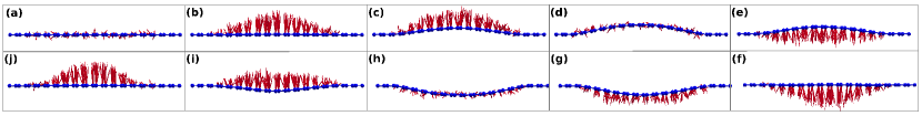
Figure 11: (Color online) The actuation of GNMR. Arrows (red online) are velocities. (a) The system is thermalized at a constant temperature 4.2 K within NVT ensemble. (b) The GNMR is actuated by adding a velocity distribution on the system. (d)-(j) The mechanical oscillation of the GNMR within NVE ensemble.

VI.2.1 Resonant Frequency and Quality Factor

There are two characteristic quantities for a nanomechanical resonator, i.e., its resonant frequency ($f$) and the Q factor. During the mechanical oscillation, the potential energy and kinetic energy exchange between each other at a frequency of $2f$. From the lattice dynamic analysis in Sec.II, we have computed the frozen frequency for the flexural mode, i.e., the frequency at zero temperature. This is an elastic property for the graphene. The temperature dependence of the flexural mode can be obtained after the consideration of the phonon-phonon scattering. The resonant frequency of a GNMR is the frequency of the flexural mode at finite temperature.

The amplitude of the mechanical oscillation decays gradually. According to this decay, the mechanical oscillation energy transforms into the random thermal vibration energy of the GNMR. The temperature increases in the system as a result of the decay of the resonant oscillation. The Q factor is directly related to the decay rate of this energy oscillation amplitude. There are several equivalent definitions for the Q factor. In MD simulations, the Q factor is usually defined with respect to the ratio of the initial mechanical oscillation energy to the dissipated energy. Its explicit formula is,Jiang et al. (2004)

$$Q=2\pi\frac{E_{\rm MR}^{0}}{\Delta E_{\rm MR}},$$

where $E_{\rm MR}^{0}$ is the initial oscillation energy. The remaining oscillation energy after $n$ cycles becomes,

$$E_{\rm MR}^{n}=E_{\rm MR}^{0}\left(1-\frac{2\pi}{Q}\right)^{n}.$$ (59)

This formula is usually applied to extract the Q factor from MD simulations.

In another alternative computation of Q factor, the resonant mechanical oscillation of the GNMR is the vibration of the flexural mode in graphene. The flexural mode has angular frequency ($\omega=2\pi f$) and lifetime ($\tau$) at finite temperature. The lifetime can be interpreted as the critical time, after which the vibration of the flexural mode decays significantly. The Q factor is essentially the total oscillation cycle number before the decay of the flexural mode,

$$Q=\omega\tau.$$ (60)

This method was used to calculate the Q factor of graphene torsional resonators.Jiang and Wang (2011c)

VI.2.2 GNMR Actuation

MD simulations and continuum elastic modeling are both useful approaches for the investigation of GNMRs. We herein demonstrate the MD simulation procedure for GNMRs. The Q factor is calculated following Eq. (59). The actuation procedure is illustrated in Fig. 11. Both left and right ends are fixed during the whole simulation. Periodic boundary condition is applied in the lateral in-plane direction. There are normally following three steps for the actuation of the GNMR.

• Firstly, Fig. 11 (a) shows the thermalization of the system to a constant pressure and temperature within the NPT (i.e. the particles number $N$, the pressure $P$, and the temperature $T$ of the system are constant) ensemble. The Nóse-HooverNose (1984); Hoover (1985) heat bath can be used to control both temperature and pressure.

• Secondly, in Fig. 11 (b), the mechanical oscillation is actuated by adding a velocity distribution to the system. The overall shape of the velocity distribution is actually the same as the morphology of the first flexural mode in graphene.

• Finally, Fig. 11 (d)-(j) display a free oscillation of the system within the NVE (i.e. the particles number $N$, the volume $V$, and the energy $E$ of the system are constant) ensemble.

Simulation data from the final NVE stage will be used in the analysis of the mechanical oscillation of the GNMR. In particular, both resonant frequency and Q-factor can be extracted from the time history of the kinetic energy.

VI.3 Energy Dissipation Mechanisms

A high Q factor is crucial for the practical application of GNMRs. Hence, it is meaningful to understand energy dissipation mechanisms for the resonant oscillation. In this section, we review some energy dissipation mechanisms in the GNMR.

Phonon-phonon scattering – This dissipation mechanism is a nonlinear effect. It is the result of the phonon-phonon scattering phenomenon. In a pure and perfect GNMR without free edge or adsorbates, the phonon-phonon scattering is the only intrinsic energy dissipation mechanism. All phonon modes are in thermal equilibrium state prior to the actuation of the mechanical oscillation. After actuation, the first flexural mode is driven into a highly non-equilibrium state. The energy of the first flexural mode will flow into the other phonon modes with the assistance of the phonon-phonon scattering. It has been shown that the flexural mode is seriously scattered by the in-plane phonon modes.Croy et al. (2012); Matheny et al. (2013) As a result, the mechanical oscillation energy of the GNMR decays and leads to the temperature increase in the system. As a result of the phonon-phonon scattering, the Q factor in the GNMR is typically inversely proportional to the temperature.Kim and Park (2009b); Jiang and Wang (2012)

Edge effect – Kim and Park pointed out the importance of the free edge on the Q factor of GNMRs.Kim and Park (2009b) The free edge is able to reduce the Q factor of the GNMR by two orders. This effect was explained in detailed by Jiang and Wang via the lattice dynamic analysis.Jiang and Wang (2012) The imaginary edge modes are found to be responsible for such a large reduction in the Q-factor. In these imaginary edge modes, the edge atoms have large vibration amplitude, while the other inner atoms has very weak vibration amplitude. Owning to its localization property, these imaginary modes will localize the thermal energy. As a result, the edge atoms will oscillate at larger amplitude than the inner atoms. It means that the edge atoms break the resonant oscillation of the whole GNMR. This contradiction leads to a fast decay of the resonant oscillation.

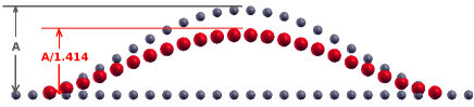
Figure 12: (Color online) Geometry of the GNMR. $A$ is the actuation amplitude. The effective amplitude is $A/\sqrt{2}$. The effective strain is determined by the difference between the length of the effective shape and the initial shape. From reference  Jiang et al., 2012.

Effective strain – In a recent work, we found that the mass sensitivity of the GNMR-based mass sensor can be enhanced by driving the resonant mechanical oscillation with large actuation energy.Jiang et al. (2012) As illustrated in Fig. 12, the oscillating GNMR shape is equivalent to a stationary shape, which is longer than the initial GNMR. The difference between the effective shape and the initial shape yields the effective strain during the resonant oscillation of the GNMR,

$$\epsilon_{\alpha}=\frac{3}{4}\pi^{2}\alpha\frac{E_{k}^{0}}{m\omega^{2}L^{2}}.$$ (61)

It was shown that this effective strain has the same effect as the mechanical strain, i.e., the frequency of the GNMR can be enhanced by the effective strain.

Adsorbate migration – The temperature dependence for the Q-factor of GNMRs has been measured by several experiments. There is an interesting scaling phenomenon. The Q-factor increases exponentially with decreasing temperature, and the exponent value will change at a transition temperature $T_{z}$.van der Zande et al. (2010); Chen et al. (2009) In a recent work, we have attributed this temperature scaling phenomenon to the adsorb migration effect on the surface of the GNMR.Jiang et al. (2014) For temperatures above $T_{z}$, the adsorb is able to move far away from the GNMR surface, and will beat the GNMR frequently. This adsorb migration effect leads to strong reduction in the Q-factor, resulting in the transition of the temperature scaling factor.

We have selectively discussed some energy dissipation mechanisms for the GNMR in the above. We concentrate on the relationship between the flexural mode and the resonant mechanical oscillation of the GNMR, which is the main focus of the present review article. There are many other interesting and important energy dissipation mechanisms for the GNMR (for review, e.g. see Ref. Imboden and Mohanty, 2013).

VII Summary and Future Prospects

In this review, we have introduced the basic lattice dynamics of the flexural mode in graphene, and summarized its important contribution to four of graphene’s thermal and mechanical properties: thermal conduction, thermal expansion, elasticity, and nanomechanical resonance.

Although fruitful progress has been achieved in the study of the flexural mode in graphene, there are still some challenges and opportunities. For example, it is a long-term and important objective to understand and develop the lattice dynamic theory, particularly in combination with the ongoing explosion in computational speed and power. As CPU speed increases, lattice dynamical properties will be able to be calculated based on first-principles simulations. These first-principles calculations can serve as an effective examination and prediction for existing results that were obtained by applying lattice dynamical theory to classical atomistic simulations.

Furthermore, the basic lattice dynamic theory can be used in conjunction to study other practical scientific problems. For example, quasi-particle phonons can be coupled with other particles like electrons and photons,Bonini et al. (2007); Mariani and Von Oppen (2008) which will be useful for studying the electronic or thermal behavior of transistor devices, whose properties and performance are governed by such interactions.

Finally, it will be important to transfer the knowledge gained regarding the important role of the flexural mode in graphene to other two-dimensional layered materials.Novoselov et al. (2005b) Inspired by the novel physical properties of two-dimensional graphene, there has been increasing interest in studying other similar two-dimensional layered materials, because these other two-dimensional materials may have superior properties to graphene. For instance, MoS₂ is a semiconductor with a bulk bandgap above 1.2 eV,Kam and Parkinson (1982); Feng et al. (2012); Lu et al. (2012) which has attracted considerable attention in recent years.Radisavljevic et al. (2011); Wang et al. (2012b); Chhowalla et al. (2013); Conley et al. (2013); Sangwan et al. (2013); Ghorbani-Asl et al. (2013); Cheiwchanchamnangij et al. (2013); Huang et al. (2013); Varshney et al. (2010); Bertolazzi et al. (2011); Cooper et al. (2013a) It is of practical significance to determine the contribution from the flexural mode to the physical properties of this, and other two-dimensional materials.

References

- Born and Huang (1954) Born, M., Huang, K.. Dynamical Theory of Crystal Lattices. Oxford University Press, Oxford; 1954.
- Landau and Lifshitz (1995) Landau, L.D., Lifshitz, E.M.. Theory of Elasticity. Pergamon,Oxford; 1995.
- Kirchhoff (1850) Kirchhoff, G.. Uber das gleichqewicht und die bewegung einer elastichen scheibe. J Reine und Angewandte Mathematik 1850;40:51–88.
- Rayleigh (1885) Rayleigh, L.. On waves propagated along the plane surface of an elastic solid. Proc London Math Soc 1885;s1-17(1):4–11.
- Lamb (1917) Lamb, H.. On waves in an elastic plate. Proc Roy Soc London, Ser A 1917;93:114–128.
- Geim and Novoselov (2007) Geim, A.K., Novoselov, K.S.. The rise of graphene. Nature Materials 2007;6(3):183–191.
- Novoselov et al. (2005a) Novoselov, K.S., Geim, A.K., Morozov, S.V., Jiang, D., Katsnelson, M.I., Grigorieva, I.V., et al. Two-dimensional gas of massless dirac fermions in graphene. Nature 2005a;438(7065):197–200.
- Balandin et al. (2008) Balandin, A.A., Ghosh, S., Bao, W., Calizo, I., Teweldebrhan, D., Miao, F., et al. Superior thermal conductivity of single-layer graphene. Nano Letters 2008;8(3):902–907.
- Nika et al. (2009a) Nika, D.L., Pokatilov, E.P., Askerov, A.S., Balandin, A.A.. Phonon thermal conduction in graphene: Role of umklapp and edge roughness scattering. Physical Review B 2009a;79:155413.
- Nika et al. (2009b) Nika, D.L., Ghosh, S., Pokatilov, E.P., Balandin, A.A.. Lattice thermal conductivity of graphene flakes: Comparison with bulk graphite. Applied Physics Letters 2009b;94(20):203103.
- Balandin (2011) Balandin, A.A.. Thermal properties of graphene and nanostructured carbon materials. Nature Materials 2011;10:569–581.
- Jiang et al. (2009a) Jiang, J.W., Wang, J.S., Li, B.. Thermal conductance of graphene and dimerite. Physical Review B 2009a;79(20):205418.
- Bao et al. (2009) Bao, W., Miao, F., Chen, Z., Zhang, H., Jang, W., Dames, C., et al. Controlled ripple texturing of suspended graphene and ultrathin graphite membranes. Nature Nanotechnology 2009;4:562–566.
- Jensen et al. (2008) Jensen, K., Kim, K., Zettl, A.. An atomic-resolution nanomechanical mass sensor. Nature Nanotechnology 2008;3:533–537.
- Tang et al. (2011) Tang, H., Wang, B.S., Su, Z.B.. Graphene Simulation, Chapter 10: Symmetry and Lattice Dynamics. InTech, Shanghai China; 2011.
- Saito et al. (1998) Saito, R., Dresselhaus, G., Dresselhaus, M.S.. Physical Properties of Carbon Nanotubes. Imperial College, London; 1998.
- Rotman (1995) Rotman, J.J.. An Introduction to the Theory of Groups. Springer-Verlag New York, Inc; 1995. ISBN 0-387-94285-8.
- Miloevic and Damnjanovic (1993) Miloevic, I., Damnjanovic, M.. Normal vibrations and Jahn-Teller effect for polymers and quasi-one-dimensional systems. Physical Review B 1993;47(13):7805–7818.
- Popov et al. (1999) Popov, V.N., Doren, V.E.V., Balkanski, M.. Lattice dynamics of single-walled carbon nanotubes. Physical Review B 1999;59(13):8355.
- Dobardzic et al. (2003) Dobardzic, E., Milosevic, I., Nikolic, B., Vukovi, T., Damnjanovic, M.. Single-wall carbon nanotubes phonon spectra: symmetry-based calculations. Physical Review B 2003;68(4):045408.
- Jiang et al. (2006) Jiang, J.W., Tang, H., Wang, B.S., Su, Z.B.. Chiral symmetry analysis and rigid rotational invariance for the lattice dynamics of single-wall carbon nanotubes. Physical Review B 2006;73(23):235434.
- Dakic et al. (2009) Dakic, B., Damnjanovic, M., Miloevic, I.. Generalized bloch states and potentials of nanotubes and other quasi-1d systems ii. Journal of Physics A: Mathematical and Theoretical 2009;42(12):125202.
- Peelaers et al. (2009) Peelaers, H., Partoens, B., Peeters, F.M.. Phonon band structure of si nanowires: A stability analysis. Nano Letters 2009;9(1):107–111.
- Liu et al. (2007) Liu, F., Ming, P., Li, J.. Ab initio calculation of ideal strength and phonon instability of graphene under tension. Physical Review B 2007;76:064120.
- Jiang (2014a) Jiang, J.W.. Phonon bandgap engineering of strained monolayer mos2. Nanoscale 2014a;6:8326.
- Kubo et al. (1992) Kubo, R., Toda, M., Hashitsume, N.. Statistical Physics II. Springer, Berlin; 1992.
- Wang and Li (2004) Wang, J.S., Li, B.. Mode-coupling theory and molecular dynamics simulation for heat conduction in a chain with transverse motions. Physical Review E 2004;70(2):021204.
- Bonini et al. (2007) Bonini, N., Lazzeri, M., Marzari, N., Mauri, F.. Phonon anharmonicities in graphite and graphene. Physical Review Letters 2007;99(17):176802.
- Mariani and Von Oppen (2008) Mariani, E., Von Oppen, F.. Flexural phonons in free-standing graphene. Physical Review Letters 2008;100(7):076801.
- Ziman (1960) Ziman, J.M.. Electrons and Phonons. Clarendon Press, Oxford; 1960.
- Cochran (1959) Cochran, W.. Theory of the lattice vibrations of germanium. Proc R Soc Ser A 1959;253:260–276.
- Martin (1969) Martin, R.M.. Dielectric screening model for lattice vibrations of diamondstructure crystals. Physical Review B 1969;186:871.
- Gale (1997) Gale, J.D.. Gulp: A computer program for the symmetry-adapted simulation of solids. J Chem Soc, Faraday Trans 1997;93(4):629–637. Code available from https://projects.ivec.org/gulp/.
- Soler et al. (2002) Soler, J.M., Artacho, E., Gale, J.D., Garcia, A., Junquera, J., Ordejon, P., et al. The siesta method for ab initio order-n materials simulation. Journal of Physics: Condensed Matter 2002;14(11):2745. Code available from http://www.icmab.es/dmmis/leem/siesta/.
- Jishi et al. (1993) Jishi, R.A., Venkataraman, L., Dresselhaus, M.S., Dresselhaus, G.. Phonon modes in carbon nanotubules. Chemical Physics Letters 1993;209(1-2):77–82.
- Aizawa et al. (1990) Aizawa, T., Souda, R., Otani, S., Ishizawa, Y.. Bond softening in monolayer graphite formed on transition-metal carbide surfaces. Physical Review B 1990;42(18):11469–11478.
- Yu (2010) Yu, P.Y.. Fundamentals of Semiconductors. Springer, New York; 2010. ISBN 978-3-642-00709-5.
- Musgrave and Pople (1962) Musgrave, M.J.P., Pople, J.A.. A general valence force field for diamond. Proc R Soc Ser A 1962;268:474–484.
- Nusimovici and Birman (1967) Nusimovici, M.A., Birman, J.L.. Lattice dynamics of wurtzite: Cds. Physical Review 1967;156(3):925–938.
- Keating (1966) Keating, P.N.. Effect of invariance requirements on the elastic strain energy of crystals with application to the diamond structure. Physical Review 1966;145(2):637–645.
- Jiang et al. (2008) Jiang, J.W., Tang, H., Wang, B.S., Su, Z.B.. A lattice dynamical treatment for the total potential energy of single-walled carbon nanotubes and its applications: relaxed equilibrium structure, elastic properties, and vibrational modes of ultra-narrow tubes. Journal of Physics: Condensed Matter 2008;20:045228.
- Brenner et al. (2002) Brenner, D.W., Shenderova, O.A., Harrison, J.A., Stuart, S.J., Ni, B., Sinnott, S.B.. A second-generation reactive empirical bond order (REBO) potential energy expression for hydrocarbons. Journal of Physics: Condensed Matter 2002;14:783–802.
- Mahan and Jeon (2004) Mahan, G.D., Jeon, G.S.. Flexure modes in carbon nanotubes. Physical Review B 2004;70:075405.
- Jiang and Wang (2010a) Jiang, J.W., Wang, J.S.. A universal exponential factor in the dimensional crossover from graphene to graphite. Journal of Applied Physics 2010a;108:124311.
- Dubay and Kresse (2003) Dubay, O., Kresse, G.. Accurate density functional calculations for the phonon dispersion relations of graphite layer and carbon nanotubes. Physical Review B 2003;67:035401.
- Mounet and Marzari (2005) Mounet, N., Marzari, N.. First-principles determination of the structural, vibrational and thermodynamic properties of diamond, graphite, and derivatives. Physical Review B 2005;71(20):205214.
- Gillen et al. (2009) Gillen, R., Mohr, M., Thomsen, C., Maultzsch, J.. Vibrational properties of graphene nanoribbons by first-principles calculations. Physical Review B 2009;80:155418.
- Metlov (2010) Metlov, K.L.. Model for flexural phonon dispersion in graphite and graphene. Physical Review B 2010;82:033404.
- Al-Jishi and Dresselhaus (1982) Al-Jishi, R., Dresselhaus, G.. Lattice-dynamical model for graphite. Physical Review B 1982;26(8):4514.
- Mohr et al. (2007) Mohr, M., Maultzsch, J., Dobardzic, E., Reich, S., Milosevic, I., Damnjanovic, M., et al. Phonon dispersion of graphite by inelastic x-ray scattering. Physical Review B 2007;76:035439.
- Stillinger and Weber (1985) Stillinger, F.H., Weber, T.A.. Computer simulation of local order in condensed phases of silicon. Physical Review B 1985;31(8):5262.
- Yien et al. (2013) Yien, S., Tayari, V., Island, J.O., Porter, J.M., Champagne, A.R.. Electronic thermal conductivity measurements in intrinsic graphene. Physical Review B 2013;87(24):241411.
- Saito et al. (2007) Saito, K., Nakamura, J., Natori, A.. Ballistic thermal conductance of a graphene sheet. Physical Review B 2007;76(11):115409.
- Schwab et al. (2000) Schwab, K., Henriksen, E.A., Worlock, J.M., Roukes, M.L.. Measurement of the quantum of thermal conductance. Nature 2000;404:974.
- Ghosh et al. (2008) Ghosh, S., Calizo, I., Teweldebrhan, D., Pokatilov, E.P., Nika, D.L., Balandin, A.A., et al. Extremely high thermal conductivity of graphene: Prospects for thermal management applications in nanoelectronic circuits. Applied Physics Letters 2008;92(15):151911.
- Xu et al. (2010) Xu, X., Wang, Y., Zhang, K., Zhao, X., Bae, S., Heinrich, M., et al. Phonon transport in suspended single layer graphene. Arxivorg 2010;.
- Mingo and Broido (2005) Mingo, N., Broido, D.A.. Carbon nanotube ballistic thermal conductance and its limits. Physical Review Letters 2005;95(9):096105.
- Xu et al. (2009) Xu, Y., Chen, X., Gu, B.L., Duan, W.. Intrinsic anisotropy of thermal conductance in graphene nanoribbons. Applied Physics Letters 2009;95(23):233116.
- Munoz et al. (2010) Munoz, E., Lu, J., Yakobson, B.I.. Ballistic thermal conductance of graphene ribbons. Nano Letters 2010;10:1652–1656.
- Wang et al. (2012a) Wang, J., Wang, X.M., Chen, Y.F., Wang, J.S.. Dimensional crossover of thermal conductance in graphene nanoribbons: a first-principles approach. Journal of Physics: Condensed Matter 2012a;24:295403.
- Nika et al. (2012) Nika, D.L., Askerov, A.S., Balandin, A.A.. Anomalous size dependence of the thermal conductivity of graphene ribbons. Nano Letters 2012;12(6):3238–3244.
- Xu et al. (2014) Xu, X., Pereira, L.F., Wang, Y., Wu, J., Zhang, K., Zhao, X., et al. Length-dependent thermal conductivity in suspended single-layer graphene. Nature Communications 2014;5:3689.
- Xiong et al. (2010a) Xiong, D., Wang, J., Zhang, Y., Zhao, H.. Heat conduction in two-dimensional disk models. Physical Review E 2010a;82:030101(R).
- Jiang et al. (2010a) Jiang, J.W., Lan, J., Wang, J.S., Li, B.. Isotopic effects on the thermal conductivity of graphene nanoribbons: Localization mechanism. Journal of Applied Physics 2010a;107(5):054314.
- Chen et al. (2012a) Chen, S., Wu, Q., Mishra, C., Kang, J., Zhang, H., Cho, K., et al. Thermal conductivity of isotopically modified graphene. Nature Materials 2012a;11:203–207.
- Yang et al. (2009) Yang, N., Zhang, G., Li, B.. Thermal rectification in asymmetric graphene ribbons. Applied Physics Letters 2009;95(3):033107.
- Hu et al. (2009) Hu, J., Ruan, X., Chen, Y.P.. Thermal conductivity and thermal rectification in graphene nanoribbons: A molecular dynamics study. Nano Letters 2009;9(7):2730–2735.
- Jiang et al. (2010b) Jiang, J.W., Wang, J.S., Li, B.. Topology-induced thermal rectification in carbon nanodevice. Europhysics Letters 2010b;89:46005.
- Jiang et al. (2010c) Jiang, J.W., Wang, J.S., Li, B.. Topological effect on thermal conductivity in graphene. Journal of Applied Physics 2010c;108:064307.
- Hu et al. (2011) Hu, J., Wang, Y., Vallabhaneni, A., Ruan, X., Chen, Y.P.. Nonlinear thermal transport and negative differential thermal conductance in graphene nanoribbons. Applied Physics Letters 2011;99(11):113101.
- Cheh and Zhao (2012) Cheh, J., Zhao, H.. Thermal rectification in asymmetric u-shaped graphene flakes. Journal of Statistical Mechanics: Theory and Experiment 2012;2012:06011.
- Ghosh et al. (2010) Ghosh, S., Bao, W., Nika, D.L., Subrina, S., Pokatilov, E.P., Lau, C.N., et al. Dimensional crossover of thermal transport in few-layer graphene. Nature Materials 2010;9:555–558.
- Singh et al. (2011) Singh, D., Murthy, J.Y., Fisher, T.S.. Mechanism of thermal conductivity reduction in few-layer graphene. Journal of Applied Physics 2011;110(4):044317.
- Lindsay et al. (2011) Lindsay, L., Broido, D.A., Mingo, N.. Flexural phonons and thermal transport in multilayer graphene and graphite. Physical Review B 2011;83:235428.
- Kong et al. (2009) Kong, B.D., Paul, S., Nardelli, M.B., Kim, K.W.. First-principles analysis of lattice thermal conductivity in monolayer and bilayer graphene. Physical Review B 2009;80:033406.
- Zhang and Zhang (2011) Zhang, G., Zhang, H.. Thermal conduction and rectification in few-layer graphene y junctions. Nanoscale 2011;3:4604.
- Zhong et al. (2011a) Zhong, W.R., Ai, M.P.Z.B.Q., Zheng, D.Q.. Chirality and thickness-dependent thermal conductivity of few-layer graphene: A molecular dynamics study. Applied Physics Letters 2011a;98(11):113107.
- Zhong et al. (2011b) Zhong, W.R., Huang, W.H., Deng, X.R., Ai, B.Q.. Thermal rectification in thickness-asymmetric graphene nanoribbons. Applied Physics Letters 2011b;99(19):193104.
- Rajabpour and Allaei (2012) Rajabpour, A., Allaei, S.M.V.. Tuning thermal conductivity of bilayer graphene by inter-layer sp3 bonding: A molecular dynamics study. Applied Physics Letters 2012;101(5):053115.
- Cao et al. (2012) Cao, H.Y., Guo, Z.X., Xiang, H., Gong, X.G.. Layer and size dependence of thermal conductivity in multilayer graphene nanoribbons. Physics Letters A 2012;376(9):525–528.
- Sun et al. (2013) Sun, T., Wang, J., Kang, W.. Van der waals interaction-tuned heat transfer in nanostructures. Nanoscale 2013;5:128.
- Jiang (2014b) Jiang, J.W.. Registry effect on the thermal conductivity of few-layer graphene. Journal of Applied Physics 2014b;116:164313.
- Yan et al. (2012) Yan, Z., Liu, G., Khan, J.M., Balandin, A.A.. Graphene quilts for thermal management of high-power gan transistors. Nature Communications 2012;3:827.
- Goyal and Balandin (2012) Goyal, V., Balandin, A.A.. Thermal properties of the hybrid graphene-metal nano-micro-composites: Applications in thermal interface materials. Applied Physics Letters 2012;100(7):073113.
- Shahil and Balandin (2012) Shahil, K.M.F., Balandin, A.A.. Graphene−multilayer graphene nanocomposites as highly efficient thermal interface materials. Nano Letters 2012;12:861–867.
- Li et al. (2010) Li, X., Maute, K., Dunn, M.L., Yang, R.. Strain effects on the thermal conductivity of nanostructures. Physical Review B 2010;81(24):245318.
- Jiang et al. (2011a) Jiang, J.W., Wang, J.S., Li, B.. A nonequilibrium green’s function study of thermoelectric properties in single-walled carbon nanotubes. Journal of Applied Physics 2011a;109:014326.
- Wei et al. (2011) Wei, N., Xu, L., Wang, H.Q., Zheng, J.C.. Strain engineering of thermal conductivity in graphene sheets and nanoribbons: a demonstration of magic flexibility. Nanotechnology 2011;22(10):105705.
- Gunawardana et al. (2012) Gunawardana, K.G.S.H., Mullen, K., Hu, J., Chen, Y.P., Ruan, X.. Tunable thermal transport and thermal rectification in strained graphene nanoribbons. Physical Review B 2012;85(24):245417.
- Zhang and Wang (2013) Zhang, J., Wang, X.. Thermal transport in bent graphene nanoribbons. Nanoscale 2013;5(2):734–743.
- Jiang et al. (2009b) Jiang, J.W., Chen, J., Wang, J.S., Li, B.. Edge states induce boundary temperature jump in molecular dynamics simulation of heat conduction. Physical Review B 2009b;80(5):052301.
- Lan et al. (2009) Lan, J., Wang, J.S., Gan, C.K., Chin, S.K.. Edge effects on quantum thermal transport in graphene nanoribbons: Tight-binding calculations. Physical Review B 2009;79(11):115401.
- Jiang and Wang (2010b) Jiang, J.W., Wang, J.S.. Conditions for the existence of phonon localized edge-modes. Physical Review B 2010b;81(17):174117.
- Savin et al. (2010) Savin, A.V., Kivshar, Y.S., Hu, B.. Suppression of thermal conductivity in graphene nanoribbons with rough edges. Physical Review B 2010;82(19):195422.
- Tan et al. (2010) Tan, Z.W., Wang, J.S., Gan, C.K.. First-principles study of heat transport properties of graphene nanoribbons. Nano Letters 2010;11(1):214–219.
- Hu et al. (2010) Hu, J., Schiffli, S., Vallabhaneni, A., Ruan, X., Chen, Y.P.. Tuning the thermal conductivity of graphene nanoribbons by edge passivation and isotope engineering: A molecular dynamics study. Applied Physics Letters 2010;97:133107.
- Jiang et al. (2011b) Jiang, J.W., Wang, J.S., Wang, B.S.. Minimum thermal conductance in graphene and boron nitride superlattice. Applied Physics Letters 2011b;99:043109.
- Jiang and Wang (2011a) Jiang, J.W., Wang, J.S.. Manipulation of heat current by the interface between graphene and white graphene. Europhysics Letters 2011a;96:16003.
- Cheh and Zhao (2011) Cheh, J., Zhao, H.. Heat conduction in graphene flakes with inhomogeneous mass interface. Journal of Statistical Mechanics: Theory and Experiment 2011;2011:10031.
- Jiang et al. (2011c) Jiang, J.W., Wang, B.S., Wang, J.S.. First principle study of the thermal conductance in graphene nanoribbon with vacancy and substitutional silicon defects. Applied Physics Letters 2011c;98:113114.
- Hao et al. (2011) Hao, F., Fang, D., Xu, Z.. Mechanical and thermal transport properties of graphene with defects. Applied Physics Letters 2011;99:041901.
- Zhang et al. (2011) Zhang, H., Lee, G., Cho, K.. Thermal transport in graphene and effects of vacancy defects. Physical Review B 2011;84:115460.
- Adamyan and Zavalniuk (2012) Adamyan, V., Zavalniuk, V.. Lattice thermal conductivity of graphene with conventionally isotopic defects. Journal of Physics: Condensed Matter 2012;24:415401.
- Serov et al. (2013) Serov, A.Y., Ong, Z.Y., Pop, E.. Effect of grain boundaries on thermal transport in graphene. Applied Physics Letters 2013;102:033104.
- Chen et al. (2012b) Chen, S., Li, Q., Zhang, Q., Qu, Y., Ji, H., Ruoff, R.S., et al. Thermal conductivity measurements of suspended graphene with and without wrinkles by micro-raman mapping. Nanotechnology 2012b;23:365701.
- Cai et al. (2010) Cai, W., Moore, A.L., Zhu, Y., Li, X., Chen, S., Shi, L., et al. Thermal transport in suspended and supported monolayer graphene grown by chemical vapor deposition. Nano Letters 2010;10:1645–1651.
- Chen et al. (2011) Chen, S., Moore, A.L., Cai, W., Suk, J.W., An, J., Mishra, C., et al. Raman measurements of thermal transport in suspended monolayer graphene of variable sizes in vacuum and gaseous environments. ACS Nano 2011;5(1):321–328.
- Lee et al. (2011) Lee, J.U., Yoon, D., Kim, H., Lee, S.W., Cheong, H.. Thermal conductivity of suspended pristine graphene measured by raman spectroscopy. Physical Review B 2011;83:081419(R).
- Guo et al. (2011) Guo, Z.X., Zhang, D., Gong, X.G.. Manipulating thermal conductivity through substrate coupling. Physical Review B 2011;84:075470.
- Ong and Pop (2011) Ong, Z.Y., Pop, E.. Effect of substrate modes on thermal transport in supported graphene. Physical Review B 2011;84(7):075471.
- Huang et al. (2011) Huang, S.Y., Wang, W.G., Kwo, S.F.L.J., Chien, C.L.. Intrinsic spin-dependent thermal transport. Physical Review Letters 2011;107:216604.
- Qiu and Ruan (2012) Qiu, B., Ruan, X.. Reduction of spectral phonon relaxation times from suspended to supported graphene. Applied Physics Letters 2012;100(19):193101.
- Guo et al. (2012) Guo, Z.X., Ding, J.W., Gong, X.G.. Substrate effects on the thermal conductivity of epitaxial graphene nanoribbons. Physical Review B 2012;85(23):235429.
- Chen et al. (2012c) Chen, S., Zhang, Y., Wang, J., Zhao, H.. Breakdown of the power-law decay prediction of the heat current correlation in one-dimensional momentum conserving lattices. arXiv:12045933 2012c;.
- Chen et al. (2013a) Chen, S., Zhang, Y., Wang, J., Zhao, H.. Why asymmetric interparticle interaction can result in convergent heat conductivity. arXiv:13097146 2013a;.
- Wang et al. (2008) Wang, J.S., Wang, J., L, J.T.. Quantum thermal transport in nanostructures. Eur Phys J B 2008;62(4):381–404.
- Wang et al. (2013) Wang, J.S., Agarwalla, B.K., Li, H., Thingna, J.. Nonequilibrium green’s function method for quantum thermal transport. Front Phys 2013;:DOI:10.1007/s11467–013–0340–x.
- Nika and Balandin (2012) Nika, D.L., Balandin, A.A.. Two-dimensional phonon transport in graphene. Journal of Physics: Condensed Matter 2012;24(23):233203.
- Cahill et al. (2003) Cahill, D.G., Ford, W.K., Goodson, K.E., Mahan, G.D., Majumdar, A., Maris, H.J., et al. Nanoscale thermal transport. Journal of Applied Physics 2003;93(2):793.
- Dhar (2008) Dhar, A.. Heat transport in low-dimensional systems. Advances in Physics 2008;57(5):457–537.
- Liu et al. (2012) Liu, S., Xu, X., Xie, R., Zhang, G., Li, B.. Anomalous heat conduction and anomalous diffusion in low dimensional nanoscale systems. Eur Phys J B 2012;85:337.
- Li et al. (2012) Li, N., Ren, J., Wang, L., Zhang, G., Hnggi, P., Li, B.. Colloquium: Phononics: Manipulating heat flow with electronic analogs and beyond. Rev Mod Phys 2012;84:1045–1066.
- Yang et al. (2012a) Yang, N., Xu, X., Zhang, G., Li, B.. Thermal transport in nanostructures. AIP Advances 2012a;2(4):041410.
- Luo and Chen (2013) Luo, T., Chen, G.. anoscale heat transfer - from computation to experiment. Phys Chem Chem Phys 2013;15(10):3389–3412.
- Marconnet et al. (2013) Marconnet, A.M., Panzer, M.A., Goodson, K.E.. Thermal conduction phenomena in carbon nanotubes and related nanostructured materials. Rev Mod Phys 2013;85:1295–1326.
- Dubi and Ventra (2011) Dubi, Y., Ventra, M.D.. Colloquium: Heat flow and thermoelectricity in atomic and molecular junctions. Rev Mod Phys 2011;83:131.
- Zhang and Li (2010) Zhang, G., Li, B.. Impacts of doping on thermal and thermoelectric properties of nanomaterials. Nanoscale 2010;2(7):1058–1068.
- Pop (2010) Pop, E.. Energy dissipation and transport in nanoscale devices. Nano Research 2010;3(3):147–169.
- Ozpineci and Ciraci (2001) Ozpineci, A., Ciraci, S.. Quantum effects of thermal conductance through atomic chains. Physical Review B 2001;63(12):125415.
- Mingo and Yang (2003) Mingo, N., Yang, L.. Phonon transport in nanowires coated with an amorphous material: An atomistic green’s function approach. Physical Review B 2003;68(24):245406.
- Yamamoto and Watanabe (2006) Yamamoto, T., Watanabe, K.. Nonequilibrium green’s function approach to phonon transport in defective carbon nanotubes. Physical Review Letters 2006;96(25):255503.
- Mingo (2006) Mingo, N.. Anharmonic phonon flow through molecular-sized junctions. Physical Review B 2006;74(12):125402.
- Spohn (2006) Spohn, H.. The phonon boltzmann equation, properties and link to weakly anharmonic lattice dynamics. Journal of Statistical Physics 2006;124:1041–1104.
- Lepri et al. (2003) Lepri, S., Livi, R., Politi, A.. Thermal conduction in classical low-dimensional lattices. Physical Review 2003;337(1):1–80.
- Wang (2007) Wang, J.S.. Quantum thermal transport from classical molecular dynamics. Physical Review Letters 2007;99:160601.
- Wang et al. (2009) Wang, J.S., Ni, X., Jiang, J.W.. Molecular dynamics with quantum heat baths: Application to nanoribbons and nanotubes. Physical Review B 2009;80(22):224302.
- Ceriotti et al. (2009a) Ceriotti, M., Bussi, G., Parrinello, M.. Langevin equation with colored noise for constant-temperature molecular dynamics simulations. Physical Review Letters 2009a;102:020601.
- Ceriotti et al. (2009b) Ceriotti, M., Bussi, G., Parrinello, M.. Nuclear quantum effects in solids using a colored-noise thermostat. Physical Review Letters 2009b;103:030603.
- Dammak et al. (2009) Dammak, H., Chalopin, Y., Laroche, M., Hayoun, M., Greffet, J.J.. Quantum thermal bath for molecular dynamics simulation. Physical Review Letters 2009;103:190601.
- Lammps (2012) Lammps, . http://wwwcssandiagov/sjplimp/lammpshtml 2012;.
- Chang et al. (2008) Chang, C.W., Okawa, D., Garcia, H., Majumdar, A., Zettl, A.. Breakdown of fourier’s law in nanotube thermal conductors. Physical Review Letters 2008;101:075903.
- Dubi and Ventra (2009) Dubi, Y., Ventra, M.D.. Fourier’s law: Insight from a simple derivation. Physical Review E 2009;79:042101.
- Yang et al. (2010) Yang, N., Zhang, G., Li, B.. Violation of fourier’s law and anomalous heat diffusion in silicon nanowires. Nanotoday 2010;5(2):85–90.
- Xiong et al. (2010b) Xiong, D., Wang, J., Zhang, Y., Zhao, H.. Heat conduction in two-dimensional disk models. Physical Review E 2010b;82(3):030101.
- Chen et al. (2013b) Chen, S., Zhang, Y., Wang, J., Zhao, H.. Diffusion of heat, energy, momentum, and mass in one-dimensional systems. Physical Review E 2013b;87(3):032153.
- Nose (1984) Nose, S.. A unified formulation of the constant temperature molecular dynamics methods. Journal of Chemical Physics 1984;81(1):511.
- Hoover (1985) Hoover, W.G.. Canonical dynamics: Equilibrium phase-space distributions. Physical Review A 1985;31(3):1695.
- Poetzsch and Bttger (1994) Poetzsch, R.H.H., Bttger, H.. Interplay of disorder and anharmonicity in heat conduction: Molecular-dynamics study. Physical Review B 1994;50(21):15757–15763.
- Jiang and Wang (2011b) Jiang, J.W., Wang, J.S.. Theoretical study of thermal conductivity in single-walled boron nitride nanotubes. Physical Review B 2011b;84(8):085439.
- Hone et al. (1999) Hone, J., Whitney, M., Zettl, A.. Thermal conductivity of single-walled carbon nanotubes. Synthetic Metals 1999;103:2498–2499.
- Gu and Chen (2007) Gu, Y., Chen, Y.. Thermal conductivities of single-walled carbon nanotubes calculated from the complete phonon dispersion relations. Physical Review B 2007;76(13):134110.
- Aksamija and Knezevic (2011) Aksamija, Z., Knezevic, I.. Lattice thermal conductivity of graphene nanoribbons: Anisotropy and edge roughness scattering. Applied Physics Letters 2011;98:141919.
- Chen and Kumar (2012) Chen, L., Kumar, S.. Thermal transport in graphene supported on copper. Journal of Applied Physics 2012;112:043502.
- Ouyang et al. (2011) Ouyang, T., Chen, Y., Xie, Y., Stocks, G.M., Zhong, J.. Thermal conductance modulator based on folded graphene nanoribbons. Applied Physics Letters 2011;99:233101.
- Yang et al. (2012b) Yang, N., Ni, X., Jiang, J.W., Li, B.. How does folding modulate thermal conductivity of graphene? Applied Physics Letters 2012b;100(9):093107.
- Amorim and Guinea (2013) Amorim, B., Guinea, F.. Flexural mode of graphene on a substrate. Physical Review B 2013;88(11):115418.
- Xu et al. (1991) Xu, C.H., Wang, C.Z., Chan, C.T., Ho, K.M.. Theory of the thermal expansion of Si and diamond. Physical Review B 1991;43(6):5024–5027.
- Wei et al. (1994) Wei, S., Li, C., Chou, M.Y.. Ab initio calculation of thermodynamic properties of silicon. Physical Review B 1994;50(19):14587–14590.
- Barrera et al. (2005) Barrera, G.D., Bruno, J.A.O., Barron, T.H.K., Allan, N.L.. Negative thermal expansion. Journal of Physics: Condensed Matter 2005;17:R217–R252.
- Yoon et al. (2011) Yoon, D., Son, Y.W., Cheong, H.. Negative thermal expansion coefficient of graphene measured by raman spectroscopy. Nano Letters 2011;11(8):3227–3231.
- Singh et al. (2010) Singh, V., Sengupta, S., Solanki, H.S., Dhall, R., Allain, A., Dhara, S., et al. Probing thermal expansion of graphene and modal dispersion at low-temperature using graphene nanoelectromechanical systems resonators. Nanotechnology 2010;21(16):165204.
- Zakharchenko et al. (2009) Zakharchenko, K.V., Katsnelson, M.I., Fasolino, A.. Finite temperature lattice properties of graphene beyond the quasiharmonic approximation. Physical Review Letters 2009;102(4):046808.
- Pozzo et al. (2011) Pozzo, M., Alfe, D., Lacovig, P., Hofmann, P., Lizzit, S., Baraldi, A.. Thermal expansion of supported and freestanding graphene: Lattice constant versus interatomic distance. Physical Review Letters 2011;106:135501.
- Jiang et al. (2009c) Jiang, J.W., Wang, J.S., Li, B.. Thermal expansion in single-walled carbon nanotubes and graphene: Nonequilibrium green’s function approach. Physical Review B 2009c;80(20):205429.
- Gruneisen (1926) Gruneisen, E.. Handbuch der Physik; vol. 10. pp 1-52; eds Geiger H (Springer, Berlin); 1926.
- Wang and Jiang (2014) Wang, J.S., Jiang, J.W.. NEGF approach and Gruneisen method for thermal expansion. in prepare 2014;.
- Li et al. (2009) Li, H., Xu, C., Srivastava, N., Banerjee, K.. Carbon nanomaterials for next-generation interconnects and passives: Physics, status, and prospects. IEEE Transactions on Electron Devices 2009;56(9):1799–1821.
- Terrones et al. (2010) Terrones, M., Botello-Méndez, A.R., Campos-Delgado, J., López-Urías, F., Vega-Cantú, Y.I., Rodríguez-Macías, F.J., et al. Graphene and graphite nanoribbons: Morphology, properties, synthesis, defects and applications. Nanotoday 2010;5(4):351–372.
- Yang et al. (2012c) Yang, Z., Gao, R., Hu, N., Chai, J., Cheng, Y., Zhang, L., et al. The prospective two-dimensional graphene nanosheets: Preparation, functionalization, and applications. Nano-Micro Letters 2012c;4(1):1–9.
- Lau et al. (2012) Lau, C.N., Bao, W., Velasco Jr., J.. Properties of suspended graphene membranes. Materials Today 2012;15(6):238–245.
- Tu and Ou-Yang (2008) Tu, Z.C., Ou-Yang, Z.C.. Elastic theory of low-dimensional continua and its applications in bio- and nano-structures. Journal of Computational and Theoretical Nanoscience 2008;5(4):422–448.
- Lu (1997) Lu, J.P.. Elastic properties of carbon nanotubes and nanoropes. Physical Review Letters 1997;79(7):1297–1300.
- Lier et al. (2000) Lier, G.V., Alsenoy, C.V., Doren, V.V., Geerlings, P.. Ab initio study of the elastic properties of single-walled carbon nanotubes and graphene. Chemical Physics Letters 2000;326:181–185.
- Kudin et al. (2001) Kudin, K.N., Scuseria, G.E., Yakobson, B.I.. C2f, bn, and c nanoshell elasticity from ab initio computations. Physical Review B 2001;64(23):235406.
- Konstantinova et al. (2006) Konstantinova, E., Dantas, S.O., Barone, P.M.V.B.. lectronic and elastic properties of two-dimensional carbon planes. Physical Review B 2006;74(3):035417.
- Reddy et al. (2006) Reddy, C.D., Rajendran, S., Liew, K.M.. Equilibrium configuration and continuum elastic properties of finite sized graphene. Nanotechnology 2006;17(3):864.
- Huang et al. (2006) Huang, Y., Wu, J., Hwang, K.C.. Thickness of graphene and single-wall carbon nanotubes. Physical Review B 2006;74:245413.
- Khare et al. (2007) Khare, R., Mielke, S.L., Paci, J.T., Zhang, S., Ballarini, R., Schatz, G.C., et al. Coupled quantum mechanical/molecular mechanical modeling of the fracture of defective carbon nanotubes and graphene sheets. Physical Review B 2007;75(7):075412.
- Wei et al. (2009) Wei, X., Fragneaud, B., Marianetti, C.A., Kysar, J.W.. Nonlinear elastic behavior of graphene: Ab initio calculations to continuum description. Physical Review B 2009;80:205407.
- Jiang et al. (2010d) Jiang, J.W., Wang, J.S., Li, B.. Elastic and nonlinear stiffness of graphene: a simple approach. Physical Review B 2010d;81(7):073405.
- Yi and Chang (2012) Yi, L., Chang, T.. Loading direction dependent mechanical behavior of graphene under shear strain. Science China Physics, Mechanics and Astronomy 2012;55(6):1083–1087.
- Zhou et al. (2013) Zhou, L., Wang, Y., Cao, G.. Elastic properties of monolayer graphene with different chiralities. Journal of Physics: Condensed Matter 2013;25:125302.
- Shenoy et al. (2008) Shenoy, V.B., Reddy, C.D., Ramasubramaniam, A., Zhang, Y.W.. Edge-stress-induced warping of graphene sheets and nanoribbons. Physical Review Letters 2008;101(24):245501.
- Duan and Wang (2009) Duan, W.H., Wang, C.M.. Nonlinear bending and stretching of a circular graphene sheet under a central point load. Nanotechnology 2009;20:075702.
- Treacy et al. (1996) Treacy, M.M.J., Ebbesen, T.W., Gibson, J.M.. Exceptionally high young’s modulus observed for individual carbon nanotubes. Nature 1996;381:678 – 680.
- Krishnan et al. (1998) Krishnan, A., Dujardin, E., Ebbesen, T.W., Yianilos, P.N., Treacy, M.M.J.. Youngs modulus of single-walled nanotubes. Physical Review B 1998;58(20):14013–14019.
- Jiang et al. (2009d) Jiang, J.W., Wang, J.S., Li, B.. Young’s modulus of graphene: a molecular dynamics study. Physical Review B 2009d;80(11):113405.
- Polyanin (2002) Polyanin, A.D.. Handbook of Linear Partial Differential Equations for Engineers and Scientists. CRC Press/CH; 2002.
- Blakslee et al. (1970) Blakslee, O.L., Proctor, D.G., Seldin, E.J., Spence, G.B., , , Weng, T.. Elastic constants of compression‐annealed pyrolytic graphite. Journal of Applied Physics 1970;41(8):3373.
- Portal et al. (1999) Portal, D., Artacho, E., Soler, J.M., Rubio, A., Ordejón, P.. Ab initio structural, elastic, and vibrational properties of carbon nanotubes. Physical Review B 1999;59(19):12678–12688.
- Reddy et al. (2009) Reddy, C.D., Ramasubramaniam, A., Shenoy, V.B., Zhang, Y… Edge elastic properties of defect-free single-layer graphene sheets. Applied Physics Letters 2009;94(10):101904.
- Cadelano et al. (2009) Cadelano, E., Palla, P.L., Giordano, S., Colombo, L.. Nonlinear elasticity of monolayer graphene. Physical Review Letters 2009;102(23):235502.
- Zhao et al. (2009) Zhao, H., Min, K., Aluru, N.R.. Size and chirality dependent elastic properties of graphene nanoribbons under uniaxial tension. Nano Letters 2009;9(8):3012–3015.
- Lee et al. (2008) Lee, C., Wei, X., Kysar, J.W., Hone, J.. Measurement of the elastic properties and intrinsic strength of monolayer graphene. Science 2008;321:385.
- Zhao and Xue (2013) Zhao, S., Xue, J.. Mechanical properties of hybrid graphene and hexagonal boron nitride sheets as revealed by molecular dynamic simulations. Journal of Physics D: Applied Physics 2013;46:135303.
- Jiang and Park (2014) Jiang, J.W., Park, H.S.. Mechanical properties of mos2/graphene heterostructures. Applied Physics Letters 2014;105:033108.
- O′Connell et al. (2010) O′Connell, A.D., Hofheinz, M., Ansmann, M., Bialczak, R.C., Lenander, M., Lucero, E., et al. Quantum ground state and single-phonon control of a mechanical resonator. Nature 2010;464:697.
- Palomaki et al. (2013) Palomaki, T.A., Harlow, J.W., Teufel, J.D., Simmonds, R.W., Lehnert, K.W.. Coherent state transfer between itinerant microwave fields and a mechanical oscillator. Nature 2013;495:210.
- Low et al. (2012) Low, T., Jiang, Y., Katsnelson, M., Guinea, F.. Electron pumping in graphene mechanical resonators. Nano Letters 2012;12(2):850–854.
- Sakhaee-Pour et al. (2008) Sakhaee-Pour, A., Ahmadian, M., Vafai, A.. Applications of single-layered graphene sheets as mass sensors and atomistic dust detectors. Solid State Communications 2008;145:168–172.
- Rumyantsev et al. (2012) Rumyantsev, S., Liu, G., Shur, M.S., Potyrailo, R.A., Balandin, A.A.. Selective gas sensing with a single pristine graphene transistor. Nano Letters 2012;12(5):2294–2298.
- Avdoshenko et al. (2012) Avdoshenko, S.M., da Rocha, C.G., Cuniberti, G.. Nanoscale ear drum: Graphene based nanoscale sensors. Nanoscale 2012;4:3168–3174.
- Midtvedt et al. (2014) Midtvedt, D., Croy, A., Isacsson, A., Qi, Z., Park, H.S.. Fermi-pasta-ulam physics with nanomechanical graphene resonators: Intrinsic relaxation and thermalization from flexural mode coupling. Physical Review Letters 2014;112:145503.
- Bunch et al. (2007) Bunch, J.S., van der Zande, A.M., Verbridge, S.S., Frank, I.W., Tanenbaum, D.M., Parpia, J.M., et al. Electromechanical resonators from graphene sheets. Science 2007;315:490.
- Robinson et al. (2008) Robinson, J.T., Zalalutdinov, M., Baldwin, J.W., Snow, E.S., Wei, Z., Sheehan, P., et al. Wafer-scale reduced graphene oxide films for nanomechanical devices. Nano Letters 2008;8(10):3441–3445.
- van der Zande et al. (2010) van der Zande, A.M., Barton, R.A., Alden, J.S., Ruiz-Vargas, C.S., Whitney, W.S., Pham, P.H.Q., et al. Large-scale arrays of single-layer graphene resonators. Nano Letters 2010;10(12):4869–4873.
- Reserbat-Plantey et al. (2012) Reserbat-Plantey, A., Marty, L., Arcizet, O., Bendiab, N., Bouchiat, V.. A local optical probe for measuring motion and stress in a nanoelectromechanical system. Nature Nanotechnology 2012;7:151–155.
- Ruiz-Vargas et al. (2011) Ruiz-Vargas, C.S., Zhuang, H.L., Huang, P.Y., van der Zande, A.M., Garg, S., McEuen, P.L., et al. Softened elastic response and unzipping in chemical vapor deposition graphene membranes. Nano Letters 2011;11:2259–2263.
- Garcia-Sanchez et al. (2008) Garcia-Sanchez, D., van der Zande, A.M., Paulo, A.S., Lassagne, B., McEuen, P.L., Bachtold, A.. Imaging mechanical vibrations in suspended graphene sheets. Nano Letters 2008;8(5):1399.
- . Girit et al. (2009) . Girit, C., Meyer, J.C., Erni, R., Rossell, M.D., Kisielowski, C., Yang, L., et al. Graphene at the edge: Stability and dynamics. Science 2009;323:1705.
- Chen et al. (2009) Chen, C., Rosenblatt, S., Bolotin, K.I., Kalb, W., Kim, P., Kymissis, I., et al. Performance of monolayer graphene nanomechanical resonators with electrical readout. Nature Nanotechnology 2009;4:861.
- Barton et al. (2011) Barton, R.A., Ilic, B., van der Zande, A.M., Whitney, W.S., Parpia, P.L.M.J.M., Craighead, H.G.. High, size-dependent quality factor in an array of graphene mechanical resonators. Nano Letters 2011;11:1232–1236.
- Croy et al. (2012) Croy, A., Midtvedt, D., Isacsson, A., Kinaret, J.M.. Nonlinear damping in graphene resonators. Physical Review B 2012;86(23):235435.
- Atalaya et al. (2008) Atalaya, J., Isacsson, A., Kinaret, J.M.. Continuum elastic modeling of graphene resonators. Nano Letters 2008;8(12):4196–4200.
- Atalaya et al. (2010) Atalaya, J., Kinaret, J.M., Isacsson, A.. Nanomechanical mass measurement using nonlinear response of a graphene membrane. Europhysics Letters 2010;91:48001.
- Kim and Park (2010) Kim, S.Y., Park, H.S.. On the utility of vacancies and tensile strain-induced quality factor enhancement for mass sensing using graphene monolayers. Nanotechnology 2010;21:105710.
- Qi and Park (2012) Qi, Z., Park, H.S.. Intrinsic energy dissipation in cvd-grown graphene nanoresonators. Nanoscale 2012;4:3460–3465.
- Kwona et al. (2012) Kwona, O.K., Leeb, G.Y., Hwangc, H.J., Kang, J.W.. Molecular dynamics modeling and simulations to understand gate-tunable graphene-nanoribbon-resonator. Physica E: Low-dimensional Systems and Nanostructures 2012;45:194–200.
- He et al. (2005) He, X.Q., Kitipornchai, S., Liew, K.M.. Resonance analysis of multi-layered graphene sheets used as nanoscale resonators. Nanotechnology 2005;16:2086–2091.
- Kim and Park (2009a) Kim, S.Y., Park, H.S.. Multilayer friction and attachment effects on energy dissipation in graphene nanoresonators. Applied Physics Letters 2009a;94:101918.
- Seonez et al. (2007) Seonez, C., Guinea, F., Neto, A.H.C.. Dissipation in graphene and nanotube resonators. Physical Review B 2007;76:125427.
- Kim and Park (2009b) Kim, S.Y., Park, H.S.. The importance of edge effects on the intrinsic loss mechanisms of graphene nanoresonators. Nano Letters 2009b;9(3):969–974.
- Jiang and Wang (2012) Jiang, J.W., Wang, J.S.. Why edge effects are important on the intrinsic loss mechanisms of graphene nanoresonators. Journal of Applied Physics 2012;111(5):054314.
- Jiang et al. (2014) Jiang, J.W., Wang, B.S., Park, H.S., Rabczuk, T.. Adsorbate migration effects on continuous and discontinuous temperature-dependent transitions in the quality factors of graphene nanoresonators. Nanotechnology 2014;25(2):025501.
- Ekinci and Roukes (2005) Ekinci, K.L., Roukes, M.L.. Nanoelectromechanical systems. Rev Sci Instrum 2005;76:061101.
- Varghese et al. (2010) Varghese, S.H., Nair, R., Nair, B.G., Hanajiri, T., Maekawa, T., Yoshida, Y., et al. Sensors based on carbon nanotubes and their applications: A review. Current Nanoscience 2010;6:331–346.
- Eom et al. (2011) Eom, K., Park, H.S., Yoon, D.S., Kwon, T.. Nanomechanical resonators and their applications in biological/chemical detection: Nanomechanics principles. Physical Review 2011;503:115–163.
- Arlett et al. (2011) Arlett, J., Myers, E., Roukes, M.. Comparative advantages of mechanical biosensors. Nature Nanotechnology 2011;6:203.
- Imboden and Mohanty (2013) Imboden, M., Mohanty, P.. Dissipation in nanoelectromechanical systems. Physics Reports 2013;534(3):89–146.
- Paulo et al. (2008) Paulo, A.S., Black, J., Garcia-Sanchez, D., Esplandiu, M.J., Aguasca, A., Bokor, J., et al. Mechanical detection and mode shape imaging of vibrational modes of micro and nanomechanical resonators by dynamic force microscopy. Journal of Physics: Conference Series 2008;100:052009.
- Unterreithmeier et al. (2010) Unterreithmeier, Q.P., Faust, T., Kotthaus, J.P.. Damping of nanomechanical resonators. Physical Review Letters 2010;105(2):027205.
- Jiang et al. (2004) Jiang, H., Yu, M.F., Liu, B., Huang, Y.. Intrinsic energy loss mechanisms in a cantilevered carbon nanotube beam oscillator. Physical Review Letters 2004;93(18):185501.
- Jiang and Wang (2011c) Jiang, J.W., Wang, J.S.. Graphene-based tortional resonator from molecular dynamics simulation. Europhysics Letters 2011c;96(6):66007.
- Matheny et al. (2013) Matheny, M.H., Villanueva, L.G., Karabalin, R.B., Sader, J.E., Roukes, M.L.. Nonlinear mode-coupling in nanomechanical systems. Nano Letters 2013;:DOI: 10.1021/nl400070e.
- Jiang et al. (2012) Jiang, J.W., Park, H.S., Rabczuk, T.. Enhancing the mass sensitivity of graphene nanoresonators via nonlinear oscillations: the effective strain mechanism. Nanotechnology 2012;23:475501.
- Novoselov et al. (2005b) Novoselov, K.S., Jiang, D., Schedin, F., Booth, T.J., Khotkevich, V.V., Morozov, S.V., et al. Two-dimensional atomic crystals. Proceedings of the National Academy of Science 2005b;102(30):10451–10453.
- Kam and Parkinson (1982) Kam, K.K., Parkinson, B.A.. Detailed photocurrent spectroscopy of the semiconducting group vi transition metal dichalcogenides. Journal of Physical Chemistry 1982;86(4):463–467.
- Feng et al. (2012) Feng, J., Qian, X., Huang, C.., Li, J.. Strain-engineered artificial atom as a broad-spectrum solar energy funnel. Nature Photonics 2012;6(12):866–872.
- Lu et al. (2012) Lu, P., Wu, X., Guo, W., Zeng, X.C.. Strain-dependent electronic and magnetic properties of mos2 monolayer, bilayer, nanoribbons and nanotubes. Phys Chem Chem Phys 2012;14(37):13035–13040.
- Radisavljevic et al. (2011) Radisavljevic, B., Radenovic, A., Brivio, J., Giacometti, V., Kis, A.. Single-layer moS2 transistors. Nature Nanotechnology 2011;6:147.
- Wang et al. (2012b) Wang, Q.H., Kalantar-Zadeh, K., Kis, A., Coleman, J.N., Strano, M.S.. Electronics and optoelectronics of two-dimensional transition metal dichalcogenides. Nature Nanotechnology 2012b;7(11):699–712.
- Chhowalla et al. (2013) Chhowalla, M., Shin, H.S., Eda, G., Li, L.., Loh, K.P., Zhang, H.. The chemistry of two-dimensional layered transition metal dichalcogenide nanosheets. Nature Chemistry 2013;5(4):263–275.
- Conley et al. (2013) Conley, H.J., Wang, B., Ziegler, J.I., Haglund, R.F., Pantelides, S.T., Bolotin, K.I.. Bandgap engineering of strained monolayer and bilayer mos2. Nano Letters 2013;13(8):3626–3630.
- Sangwan et al. (2013) Sangwan, V.K., Arnold, H.N., Jariwala, D., Marks, T.J., Lauhon, L.J., Hersam, M.C.. Low-frequency electronic noise in single-layer mos2 transistors. Nano Letters 2013;13(9):4351–4355.
- Ghorbani-Asl et al. (2013) Ghorbani-Asl, M., Zibouche, N., Wahiduzzaman, M., Oliveira, A.F., Kuc, A., Heine, T.. Electromechanics in mos2 and ws2: Nanotubes vs. monolayers. Scientific Reports 2013;3:2961.
- Cheiwchanchamnangij et al. (2013) Cheiwchanchamnangij, T., Lambrecht, W.R.L., Song, Y., Dery, H.. Strain effects on the spin-orbit induced band structure splittings in monolayer mos2 and graphene. Physical Review B 2013;88:155404.
- Huang et al. (2013) Huang, W., Da, H., Liang, G.. Thermoelectric performance of mx2 (m=mo, w; x=s, se) monolayers. Journal of Applied Physics 2013;113:104304.
- Varshney et al. (2010) Varshney, V., Patnaik, S.S., Muratore, C., Roy, A.K., Voevodin, A.A., Farmer, B.L.. Md simulations of molybdenum disulphide (mos2): Force-field parameterization and thermal transport behavior. Computational Materials Science 2010;48(1):101–108.
- Bertolazzi et al. (2011) Bertolazzi, S., Brivio, J., Kis, A.. Stretching and breaking of ultrathin mos2. ACS Nano 2011;5(12):9703–9709.
- Cooper et al. (2013a) Cooper, R.C., Lee, C., Marianetti, C.A., Wei, X., Hone, J., Kysar, J.W.. Nonlinear elastic behavior of two-dimensional molybdenum disulfide. Physical Review B 2013a;87:035423.