Critical behavior and universality properties of uniaxial ferromagnetic thin films in the presence of random magnetic fields

Abstract

Critical phenomena in uniaxial ferromagnetic thin films in the presence of random magnetic fields have been studied within the framework of effective field theory. When the type of the random field distribution is bimodal, the system exhibits tricritical behavior. Furthermore, the critical value of surface to bulk ratio of exchange interactions at which the transition temperature becomes independent of film thickness is insensitive to the presence of disorder whether the distribution is bimodal or trimodal. Regarding the universality properties, neither $p$, nor $h$ variations in the system can affect the value of the shift exponent $\lambda$. In this regard, it can be concluded that pure ferromagnetic thin films are in the same universality class with those under the influence of random discrete magnetic fields.

I Introduction

The surface magnetism which was proposed approximately four decades ago from present by Mills mills0 ; mills1 is still one of the most actively studied research fields in statistical mechanics of phase transitions and critical phenomena kaneyoshi1 ; pleimling0 . The reason is due to the fact that in the presence of free surfaces, magnetic properties of thin films drastically differ from those of bulk materials. In other words, due to their reduced coordination number, the surface atoms have less translational symmetry and the exchange interaction between two adjacent surface atoms is different than that of the inner atoms kaneyoshi2 . As a consequence of these facts, the surface may exhibit an ordered phase even if the bulk itself is disordered. This phenomenon has already been experimentally observed ran ; polak ; tang . In this context, an extraordinary case is defined as the transition at which the surface becomes disordered at a particular temperature $T_{c}^{s}$ which is larger than the bulk transition temperature $T_{c}^{b}$, on the contrary, in an ordinary case, bulk region orders when the surface is disordered.

It is theoretically predicted that there exists a critical value of surface to bulk ratio of exchange interactions $R_{c}$ above which the surface effects are dominant and the transition temperature of the entire film is determined by the surface magnetization whereas below $R_{c}$, the transition characteristics of the film are governed by the bulk magnetization. The critical value $R_{c}$ itself is called as the special point, and the numerical value of this point has been examined within various theoretical techniques based on several extensions of an Ising type spin Hamiltonian aguilera ; binder ; kaneyoshi3 ; kaneyoshi4 ; burkhardt ; landau ; sarmento0 ; neto ; tucker . Among these works, within the framework of effective field theory (EFT), Sarmento and Tucker sarmento0 clarified that a transverse field in the surface layer causes the critical value of the surface exchange enhancement $R_{c}$ to move to a higher value whereas the presence of a bulk transverse field causes $R_{c}$ to decrease to a lower value. In addition, using extensive Monte Carlo (MC) simulations, the effect of surface exchange enhancement on ultra thin spin-1 films has been studied by Tucker tucker , and it was concluded that the $R_{c}$ value is spin dependent. Moreover, in a very recent work, the problem has also been handled for the systems in the presence of quenched dilute and trimodal random crystal fields within the framework of EFT, and it has been reported that the $R_{c}$ value can be modified in the presence of crystal field disorder yuksel0 .

In a recent paper, regarding the presence of random magnetic fields, the effect of Gaussian random longitudinal magnetic field distribution on the phase diagrams and magnetization behavior of the transverse Ising thin film have been investigated, and it has been shown that phase diagrams of the model exhibit only second-order phase transition properties, and changing the width $\sigma$ of the random field distribution makes no significant change in $R_{c}$ akinci .

On the other hand, theoretical and experimental investigations are also focused on the finite size shift of the critical temperature of the film as a function of its thickness which is characterized by a shift exponent $\lambda$. A number of experimental studies have been devoted to determine the value of $\lambda$ for various thin film samples, and it has been concluded that the shift exponent extends from $\sim 1$ to $3.15$ farle ; elmers ; henkel ; ballentine . Since the exponent $\lambda$ is directly related on the bulk correlation length exponent as $\nu_{b}=1/\lambda$ barber0 , within the accuracy of Ising-type models, it can be mentioned that a sample of thin film for which the exponent $\lambda$ is close to unity exhibits a two dimensional character whereas as the value of the exponent becomes larger than unity then the system shows a three dimensional character. Theoretically, the exponent $\lambda$ has been extracted for some certain models with a wide variety of techniques. For instance, using the high temperature series expansion (HTSE) method, it has been shown that the estimated value of $\lambda$ for ferromagnetic Ising allan ; capehart and Heisenberg ritchie thin films severely depends on whether a periodic or free boundary condition was considered in the surface. This result has also been verified within the resolution of MC simulations binder2 ; kitatani ; takamoto ; laosiritaworn . Moreover, the value of the extracted exponent is also very sensitive to the lattice geometry masrour .

Under certain circumstances, universal behavior of a thin film system may experience a dimensional crossover. Such a phenomenon has been experimentally observed as the film thickness is varied in ultra-thin $\mathrm{Ni}(111)$ films on $\mathrm{W}(110)$ li , and epitaxial thin films of Co, Ni, and their alloys grown on $\mathrm{Cu}(100)$ and $\mathrm{Cu}(111)$ huang . Previous MC simulations binder also predict that the exponent $\lambda$ may vary continuously with surface exchange $J_{s}$ in the range $R<R_{c}$ which also indicates the occurrence of a dimensional crossover between the surface value and bulk value.

In our previous work yuksel1 , with using EFT, we have studied the universal behavior and critical phenomena in a ferromagnetic thin film described by a spin-1 Blume-Capel Hamiltonian yuksel1 and we have found that the critical value of surface to bulk ratio of exchange interactions $R_{c}$ strictly depends on the crystal field interactions. On the other hand, our numerical results yield that in terms of the exponent $\lambda$, a ferromagnetic spin-1/2 thin film is in the same universality class with its spin-1 counterpart.

Based on these circumstances, in the present paper, we extended our study, and we investigated the phase transition properties of ferromagnetic uniaxial Ising thin films in the presence of random magnetic fields. We also extracted the shift exponent for the present model, and discussed the universality properties of the system in the presence of random fields by examining the variation of the exponent $\lambda$ as a function of random field parameters.

The organization of the paper is as follows: In Section II we briefly present the formulations. The results and discussions are presented in Section III, and finally Section IV contains our conclusions.

II Model and Formulation

We consider a ferromagnetic thin film with thickness $L$ in the presence of random magnetic fields described by the following Hamiltonian

$$\mathcal{H}=-\sum_{<ij>}J_{ij}S_{i}S_{j}-\sum_{i}h_{i}S_{i},$$ (1)

where $J_{ij}=J_{s}$ if the lattice sites $i$ and $j$ belong to one of the two surfaces of the film, otherwise we have $J_{ij}=J_{b}$ where $J_{s}$ and $J_{b}$ denote the ferromagnetic surface and bulk exchange interactions, respectively. The first term in Eq. (1) is a summation over the nearest-neighbor spins with $S_{i}=\pm 1$ and the second term represents the Zeeman energy originating from spatially random magnetic fields on the lattice which are distributed according to a given probability distribution function. The present study deals with a trimodal distribution which is defined as

$$P(h_{i})=p\delta(h_{i})+\left(\frac{1-p}{2}\right)[\delta(h_{i}-h_{0})+\delta(h_{i}+h_{0})].$$ (2)

According to Eq. (2), we have a pure system for $p=1.0$, whereas as $p$ approaches to zero, the form of the random field distribution becomes a bimodal-type where half of the lattice sites are subject to a magnetic field $-h_{0}$ and the remaining lattice sites have a field $h_{0}$. Then $p$ can be regarded as an adjustable parameter which controls the amount of disorder in the system.

The magnetizations $m_{i}$ ($i=1,...,L$) perpendicular to the surface of the film corresponding to $L$ parallel distinct layers can be obtained by conventional EFT formulation based on differential operator technique and decoupling approximation (DA) kaneyoshi0

$$m_{1} = [A_{1}+m_{1}B_{1}]^{z}[A_{2}+m_{2}B_{2}]F(x)|_{x=0},$$

$$m_{l} = [A_{2}+m_{l}B_{2}]^{z}[A_{2}+m_{l-1}B_{2}][A_{2}+m_{l+1}B_{2}]F(x)|_{x=0},$$

$$m_{L} = [A_{1}+m_{L}B_{1}]^{z}[A_{2}+m_{L-1}B_{2}]F(x)|_{x=0},$$ (3)

where $2\leq l\leq L-1$, and the coefficients $A_{i}$ and $B_{i}$ are defined as $A_{1}=\cosh(J_{s}\nabla)$, $A_{2}=\cosh(J_{b}\nabla)$, $B_{1}=\sinh(J_{s}\nabla)$ and $B_{2}=\sinh(J_{b}\nabla)$. In the present work, we will focus on the ferromagnetic films in a simple cubic lattice structure, i.e. $z=4$ where $z$ is the intra-layer coordination number. The function $F(x)$ in Eq. (II) is then given by

$$F(x)=\int dh_{i}P(h_{i})\tanh[\beta(x+h_{i})],$$ (4)

where $\beta$ is the inverse of the reduced temperature.

Using the Binomial expansion

$$(x+y)^{n}=\sum_{i=0}^{n}\left(\begin{tabular}[]{c }n\\ i\\ \end{tabular}\right)x^{n-i}y^{i},$$ (5)

in Eq. (II) we get

$$m_{1} = \sum_{i=0}^{z}\sum_{j=0}^{1}K_{1}(i,j)m_{1}^{i}m_{2}^{j},$$

$$m_{l} = \sum_{i=0}^{z}\sum_{j=0}^{1}\sum_{k=0}^{1}K_{2}(i,j,k)m_{l}^{i}m_{l-1}^{j}m_{l+1}^{k},$$

$$m_{L} = \sum_{i=0}^{z}\sum_{j=0}^{1}K_{1}(i,j)m_{L}^{i}m_{L-1}^{j},$$ (6)

where

$$K_{1}(i,j) = \left(\begin{tabular}[]{c}z\\ i\\ \end{tabular}\right)A_{1}^{z-i}A_{2}^{1-j}B_{1}^{i}B_{2}^{j}F(x)|_{x=0},$$ (9)

$$K_{2}(i,j,k) = \left(\begin{tabular}[]{c}z\\ i\\ \end{tabular}\right)A_{2}^{z+2-i-j-k}B_{2}^{i+j+k}F(x)|_{x=0}.$$ (12)

Consequently, applying the Binomial expansion for the coefficients $A_{i}$ and $B_{i}$ $(i=1,2)$ in Eq. (9) yields

$$K_{1}(i,j) = \left(\begin{tabular}[]{c}z\\ i\\ \end{tabular}\right)2^{-(z+1)}\sum_{x=0}^{z-i}\sum_{y=0}^{1-j}\sum_{r=0}^{i}\sum_{t=0}^{j}(-1)^{t+r}\left(\begin{tabular}[]{c }z-i\\ x\\ \end{tabular}\right)\left(\begin{tabular}[]{c }1-j\\ y\\ \end{tabular}\right)\left(\begin{tabular}[]{c }i\\ r\\ \end{tabular}\right)\left(\begin{tabular}[]{c }j\\ t\\ \end{tabular}\right)$$

$$\times\exp[(z-2r-2x)J_{s}\nabla]\exp[(1-2y-2t)J_{b}\nabla]F(x)|_{x=0},$$

$$K_{2}(i,j,k) = \left(\begin{tabular}[]{c}z\\ i\\ \end{tabular}\right)2^{-(z+2-2k)}\sum_{x=0}^{(z+2-i-j-k)}\sum_{y=0}^{(i+j-k)}(-1)^{y}\left(\begin{tabular}[]{c }z+2-i-j-k\\ x\\ \end{tabular}\right)\left(\begin{tabular}[]{c }i+j-k\\ y\\ \end{tabular}\right)$$ (31)

$$\times\exp[(z+2-2k-2x-2y)J_{b}\nabla]F(x)|_{x=0}.$$

With the help of the relation $\exp(\alpha\nabla)F(x)=f(x+\alpha)$ for an arbitrary $\alpha$, the coefficients $K_{1}$ and $K_{2}$ can be numerically evaluated. Hence, by inserting Eq. (II) in Eq. (II) we obtain a system of coupled non-linear equations which contains $L$ unknowns which are nothing but just the layer magnetizations of the film. The longitudinal magnetization $m_{i}$ of each layer can be obtained from numerical solution of Eq. (II). Then the bulk and surface magnetizations of a ferromagnetic thin film can be defined as

$$m_{b}=\frac{1}{L-2}\sum_{i=2}^{L-1}m_{i},\quad m_{s}=\frac{1}{2}(m_{1}+m_{L}).$$ (32)

Since, the magnetization of the entire system is close to zero in the vicinity of the second order phase transition, the transition temperature can be obtained by linearizing Eq. (II), i.e.

$$m_{1} = K_{1}(1,0)m_{1}+K_{1}(0,1)m_{2},$$

$$m_{l} = K_{2}(1,0,0)m_{l}+K_{2}(0,1,0)m_{l-1}+K_{2}(0,0,1)m_{l+1},$$

$$m_{L} = K_{1}(1,0)m_{L}+K_{1}(0,1)m_{L-1}.$$ (33)

Critical temperature as a function of the system parameters can be determined from $\mathrm{det}(A)=0$ where $A$ is the coefficients matrix of the set of $L$ linear equations in Eq. (II). We note that the determination of the transition temperature should be treated carefully since as it was previously stated in Ref. sarmento0 , from the many formal solutions of $\mathrm{det}(A)=0$, we have to choose the one corresponding to the highest possible transition temperature. At this point, we should also note that transition temperature $T_{c}(\infty)$ of the bulk ferromagnetic system in the presence of random fields can be evaluated by solving the following equation kaneyoshi0

$$1=q\cosh^{q-1}(J_{b}\nabla)\sinh(J_{b}\nabla)F(x)|_{x=0},$$ (34)

where $J_{b}$ is the ferromagnetic bulk exchange interaction, and $q=6$ corresponding to simple cubic lattice structure.

According to the finite-size scaling theory barber0 , the deviation of the thickness dependent critical temperature $T_{c}(L)$ of a thin ferromagnetic film from the bulk critical temperature $T_{c}(\infty)$ can be measured for sufficiently thicker films in terms of a scaling relation:

$$\varepsilon=1-T_{c}(L)/T_{c}(\infty)\propto L^{-\lambda},$$ (35)

where $\lambda$ is called the shift exponent which is related to the correlation length exponent of the bulk system as $\lambda=1/\nu_{b}$. The exponent $\lambda$ can be extracted from numerical data by plotting $\varepsilon$ versus $L$ curves for sufficiently thick films in a log-log scale then fitting the resultant curve using the standard linear regression method.

III Results and Discussion

In this section, we will discuss how the presence of random fields affects the critical and universal behavior of ferromagnetic uniaxial thin films. Before proceeding, let us note that the adjustable system parameters such as temperature, magnetic field, and surface exchange couplings are measured in terms of the bulk exchange interactions. Hence, we use the following dimensionless variables in our calculations: The temperature is defined as $k_{B}T/J_{b}$, magnetic field is scaled as $h=h_{0}/J_{b}$, and the surface exchange interactions are defined as $R=J_{s}/J_{b}$.

When the variation of the transition temperature of a ferromagnetic thin film is plotted as a function of $R$ for different film thickness $L$, at a particular $R=R_{c}$ value, the transition temperature becomes independent of film thickness. For $R<R_{c}$ (ordinary case), bulk is magnetically dominant against surface whereas for $R>R_{c}$ (extraordinary case), ferromagnetism of surface is enhanced in comparison with the bulk magnetization. In the ordinary case, thicker films exhibit greater transition temperatures while in the extraordinary case, one has just the opposite scenario.

After this short summary, let us divide our study into two parts: First, we will focus our attention on the effect of random fields which are distributed according to a symmetric bimodal distribution which can be achieved by putting $p=0$ in Eq. (2), then we will generalize the study for trimodal random fields where we can use arbitrary $p$ values within the range $0\leq p\leq 1$.

III.1 Bimodal distribution

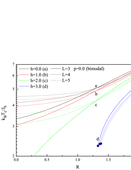
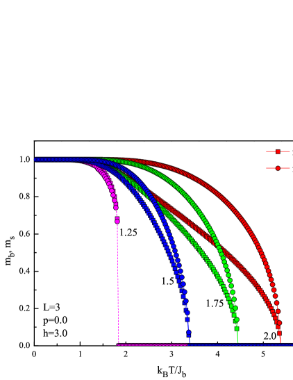
Figure 1: (a) Phase diagrams of the system in a $(k_{B}T_{c}/J_{b}-R)$ plane for various film thickness $L$ corresponding to bimodal random field distribution with $h=0.0$, $1.0$, $2.0$ and $3.0$. Solid circles denote the tricritical points. (b) Thermal variation of bulk (filled squares) and surface (filled circles) magnetizations. The numbers accompanying the curves denote the value of the reduced surface exchange interaction $R$.

From Eq. (2), we can see that a bimodal distribution of random fields is governed by only one parameter which is the external field value $h$. In Fig. 1a, in order to see the effect of external field $h$ on the critical behavior of the system, we plot the phase diagrams in a $(k_{B}T_{c}/J_{b}-R)$ plane with different film thickness $L$ and for some selected $h$ values. As seen in this figure, transition temperature of the films with the same thickness $L$ decreases with increasing disorder (i.e. as $h$ increases). However, the location of $R_{c}$ does not exhibit any significant variation with increasing $h$. In other words, $R_{c}=1.3068$ value obtained for pure films kaneyoshi4 is independent of the magnetic field disorder. However, for sufficiently high $h$ values such as $h=3.0$, randomness effects become prominent. Consequently, the curves with different $L$ values do not intersect each other, and the system reaches to its ferromagnetic phase stability limit by exhibiting a tricritical behavior.

The linearized equations given in Eq. (II) are inapplicable for the first order transitions. However, these unstable solutions can be located by examining the discontinuous jumps in thermal dependence of magnetization curves (c.f. Fig. 1b). We believe that the tricritical behavior observed in this case originates from the type of the random field distribution. Namely, the existence of tricritical point may be explained by the following physical reason: When the distribution of random magnetic fields is bimodal, there exist two equal positive and negative large fields. If these large magnetic fields are dominant against the ferromagnetic exchange interactions such as $h=3.0>>R$, in this case, spin-up and spin-down states are canceled out, and the overall system behaves like spin-$0$. This concept is very similar to that observed in the spin-1 Ising system, when the crystal field $D$ takes a large negative critical value kaneyoshi0 . Besides, in the presence of a continuous probability distribution such as a Gaussian, the system has been found to exhibit only second order phase transitions akinci . Moreover, similar arguments have also been reported for bulk systems for which different random field distributions lead to different phase diagrams yuksel2 .

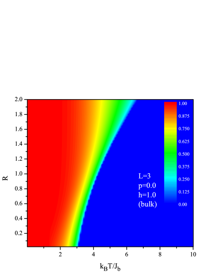
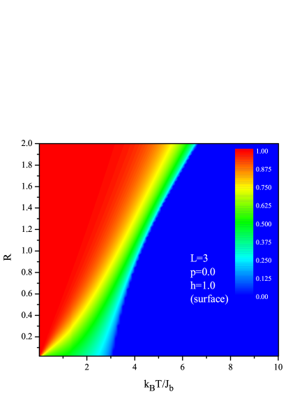
Figure 2: Contour plot projections of bulk (left panel) and surface (right panel) magnetizations of a thin ferromagnetic film with $L=3$ in a $(R-k_{B}T/J_{b})$ plane corresponding to the phase diagram with $h=1.0$ curve depicted in Fig. 1a.

Bulk and surface magnetization profiles as functions of the temperature and reduced surface exchange interactions are illustrated in Fig. 2 for $L=3$ and $h=1.0$ corresponding to the curves depicted in Fig. 1a. For weak $R$ values, ferromagnetism in the bulk region of the film is enhanced against the surface. However, as $R$ has a value far above $R_{c}$, ferromagnetic order at the surface region of the film becomes dominant against the bulk region.

Now, let us discuss the universality properties of the system in the presence of bimodal random fields. In our previous work yuksel1 , we have found that ferromagnetic thin films may exhibit dimensional crossover as $R$ changes. Namely, as we stated before, as the value of the shift exponent $\lambda$ approaches to unity then the system has a two dimensional behavior which is a direct consequence of the surface exchange enhancement whereas as the bulk region becomes dominant against the surface, $\lambda$ becomes larger than unity, and the system shows three dimensional character. In this context, our previous work yields that for $R=0.5$, we obtain $\lambda=2.01$, for $R=1.0$ the exponent value is $\lambda=1.87$, and for $R=1.3$, we have $\lambda=1.08$ yuksel1 . These exponent values were extracted for pure system. However, as shown in Fig. 3, the exponent $\lambda$ is independent of the randomness. We note that in order to precisely cover the critical region, the obtained data have been fitted for those providing the condition $0.01\leq\varepsilon\leq 0.1$ binder2 which generally requires to consider the transition temperatures of the films with $L\geq 10$ in fitting procedure. Extracted exponent values are summarized in Table-1 for a variety of set of system parameters.

III.2 Trimodal distribution

Up to now, we have considered the presence of bimodal random fields. In a trimodal random field distribution, in addition to the magnetic field strength $h$, there is another parameter $p$ which controls the amount of disorder acting on the system. According to Eq. (2), we have a pure system for $p=1.0$ whereas as $p$ decreases, then the effect of the bimodal random fields gradually becomes dominant. In Fig. 4, phase diagrams in a $(k_{B}T_{c}/J_{b}-R)$ plane are plotted for the films with different thickness $L$ with a variety of $p$ values. By comparing Figs. 4a-4c, we see that the phase diagrams corresponding to bimodal curves with $p=0$ evolve into pure system with increasing $p$. When $p=0$, disorder is maximum, hence as $p$ increases, disorder effects are cleansed, tricritical points which are observed in bimodal disorder configurations disappear, and the transition temperature increases. However, the location of $R_{c}$ is insensitive to the presence of disorder whether the distribution is bimodal or trimodal.

As a complementary investigation, bulk and surface magnetizations with $L=3$ thick films in the presence of trimodal random fields with $h=2.0$ as functions of disorder parameter $p$ and reduced temperature $k_{B}T/J_{b}$ are shown in Fig. 5. As expected, bulk (surface) region of the film is magnetically dominant in ordinary (extraordinary) case. We can also conclude from this figure that the transition temperature exhibits very slow variation with disorder parameter $p$.

Finally, in Fig. 6, we examine the influence of trimodal random fields on the shift exponent $\lambda$. One can easily conclude from this figure that neither $p$, nor $h$ variations in the system can affect the value of the shift exponent $\lambda$ (see Table-1). Although the situation is depicted for moderate values of reduced surface exchange interactions such as $R=1.0$, our numerical data yield the same conclusion for any arbitrary $R<R_{c}$ values.

IV Conclusions

In conclusion, we have presented some results regarding the critical behavior and universality properties of uniaxial ferromagnetic thin films in the presence of bimodal and trimodal random fields. We have given proper phase diagrams, magnetization profiles and variation of the shift exponent $\lambda$ as a function of system parameters.

In our recent papers yuksel0 ; yuksel1 , we have found that critical value of surface exchange coupling $R_{c}$ is a spin dependent property, and variation of crystal field interactions, as well as the presence of random crystal fields clearly affects the value of $R_{c}$. However, the shift exponent $\lambda$ has been found to be a spin ”independent” property. Therefore, we have concluded that a ferromagnetic spin-1/2 thin film is in the same universality class with its spin-1 counterpart.

On the other hand, the main findings of the present work can be summarized as follows:

• In the presence of bimodal random fields, the system exhibits tricritical behavior for sufficiently large magnetic field strengths. However, the linearized equations given in Eq. (II) are inapplicable for the first order transitions, and according to us, the tricritical behavior is a consequence of the nature of the bimodal random field distribution.

• The location of $R_{c}$ at which the transition temperature becomes independent of film thickness $L$ is insensitive to the presence of disorder whether the distribution is bimodal or trimodal.

• Regarding the universality properties, neither $p$, nor $h$ variations in the system can affect the value of the shift exponent $\lambda$. In light of these findings, we can conclude that in the context of the shift exponent, universality class of uniaxial ferromagnetic thin films is independent of the presence of random magnetic fields.

We hope that the results presented in the present paper constitute some preliminary ideas for future works based on more sophisticated techniques.

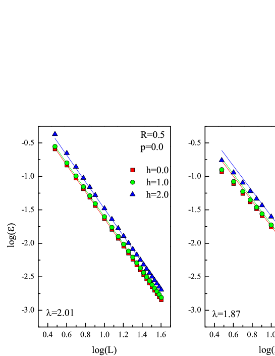
Figure 3: Variation of the shift exponent $\lambda$ for weak (left panel) and moderate (right panel) surface couplings corresponding to bimodal distribution of random fields with some selected values of magnetic field $h$.

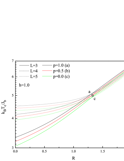
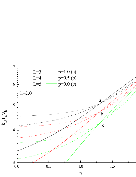
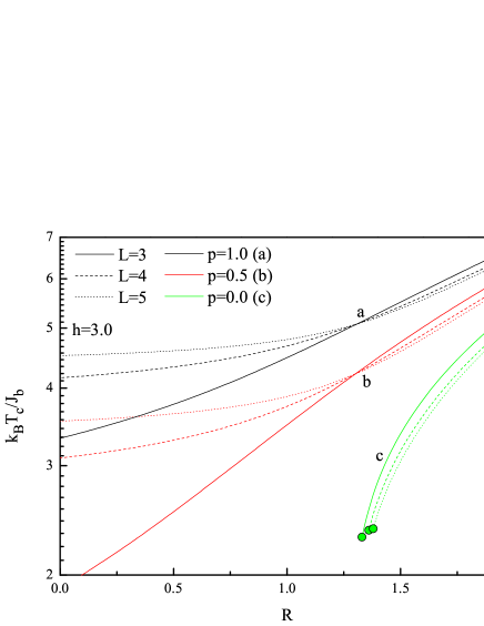
Figure 4: Phase diagrams of the system in a $(k_{B}T_{c}/J_{b}-R)$ plane for various film thickness $L$ corresponding to trimodal random field distribution with (a) $h=1.0$, (b) $2.0$, (c) $3.0$. The letters on each set of curves denote the amount of disorder $p$. Solid circles denote the tricritical points.

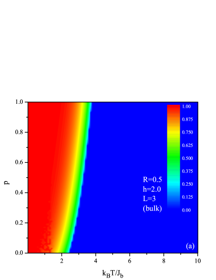
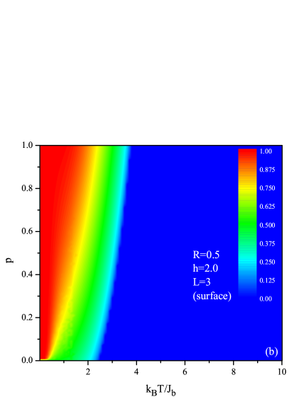
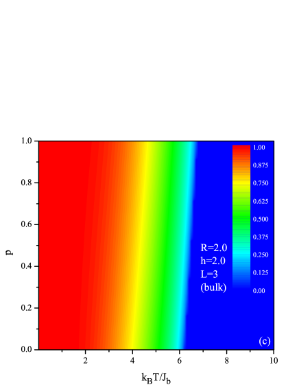
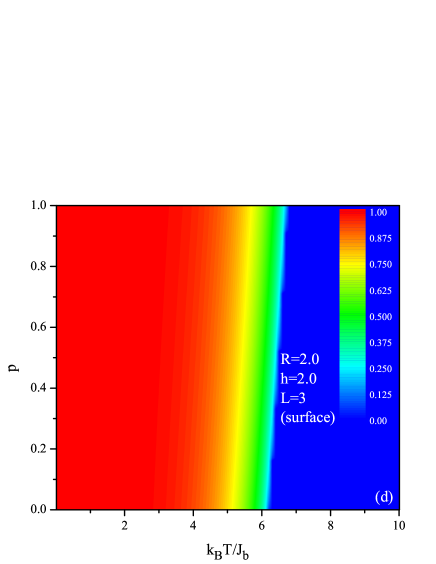
Figure 5: Contour plot projections of bulk and surface magnetizations in a $(p-k_{B}T/J_{b})$ plane with $L=3$ and $h=2.0$ in the presence of (a), (b) reduced $(R=0.5)$ and (c), (d) enhanced $(R=2.0)$ surface interactions.

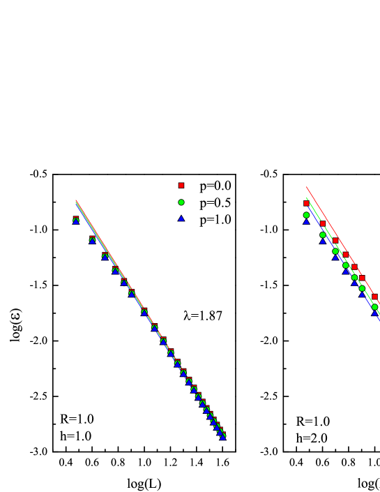
Figure 6: Variation of the shift exponent $\lambda$ for moderate surface coupling corresponding to some selected values of disorder parameter $p$ with $h=1.0$ (left panel) and $h=2.0$ (right panel).

Table 1: The list of the extracted shift exponent $\lambda$ values for several sets of random field parameters $h$ and $p$ in the presence of weak $(R=0.5)$ and moderate $(R=1.0)$ surface couplings. Corresponding residual error values due to fitting procedure are also listed in the rightmost column.

$R$	$h$	$p$	$\lambda$	error
0.5	0.0 (1.0, 2.0)	0.0 (1.0)	2.01	$2.0\times 10^{-3}$
0.5	1.0	0.0	2.01	$9.72\times 10^{-4}$
0.5	2.0	0.0	2.01	$6.23\times 10^{-4}$
1.0	0.0	0.0	1.87	$6.0\times 10^{-3}$
1.0	1.0	0.0	1.87	$4.7\times 10^{-4}$
1.0	2.0	0.0	1.87	$6.0\times 10^{-3}$
1.0	1.0	0.5	1.87	$4.47\times 10^{-5}$
1.0	2.0	0.5	1.87	$5.95\times 10^{-5}$

References

- (1) D. L. Mills, Phys. Rev. B 3 (1971) 3887.
- (2) D. L. Mills, Phys. Rev. B 8 (1973) 4424.
- (3) T. Kaneyoshi, J. Phys.: Condens. Matter 3 (1991) 4497.
- (4) M. Pleimling, J. Phys. A: Math. Gen. 37 (2004) R79, and the references therein.
- (5) T. Kaneyoshi, Introduction to Surface Magnetism, CRC Press, Boston, 1991.
- (6) C. Ran, C. Jin, M. Roberts, J. Appl. Phys. 63 (1988) 3667.
- (7) M. Polak, L. Rubinovich, J. Deng, Phys. Rev. Lett. 74 (1995) 4059.
- (8) H. Tang, Phys. Rev. Lett. 71 (1985) 444.
- (9) F. Aguilera-Granja, J. L. Morán-López, Solid State Commun. 74 (1990) 155.
- (10) K. Binder, P. C. Hohenberg, Phys. Rev. B 9 (1974) 2194.
- (11) T. Kaneyoshi, I. Tamura, E. F. Sarmento, Phys. Rev. B 28 (1983) 6491.
- (12) T. Kaneyoshi, Physica A 319 (2003) 355.
- (13) T. W. Burkhardt, E. Eisenriegler, Phys. Rev. B 16 (1977) 3213.
- (14) D. P. Landau, K. Binder, Phys. Rev. B 41 (1990) 4633.
- (15) E. F. Sarmento, J. W. Tucker, J. Magn. Magn. Mater. 118 (1993) 133.
- (16) J. C. Neto, J. R. de Sousa, J. A. Plascak, Phys. Rev. B 66 (2002) 064417.
- (17) J. W. Tucker, J. Magn. Magn. Mater. 210 (2000) 383.
- (18) Y. Yüksel, Physica A 396 (2014) 9.
- (19) Ü. Akıncı, J. Magn. Magn. Mater. 329 (2013) 178.
- (20) M. Farle, K. Baberschke, Phys. Rev. Lett. 58 (1987) 511.
- (21) H. J. Elmers, J. Hauschild, H. Höche, U. Gradmann, H. Bethge, D. Heuer, U. Köhler, Phys. Rev. Lett. 73 (1994) 898.
- (22) M. Henkel, S. Andrieu, P. Bauer, M. Piecuch, Phys. Rev. Lett. 80 (1998) 4783.
- (23) C. A. Ballentine, R. L. Fink, J. A. Pochet, J. L. Erskine, Phys. Rev. B 41 (1990) 2631.
- (24) M. N. Barber, in: J. L. Lebowitz (Ed.), Phase Transitions and Critical Phenomena, vol. 8, Academic, London, 1983.
- (25) G. A. T. Allan, Phys. Rev. B 1 (1970) 352.
- (26) T. W. Capehart, M. E. Fisher, Phys. Rev. B 13 (1976) 5021.
- (27) D. S. Ritchie, M. E. Fisher, Phys. Rev. B 7 (1973) 480.
- (28) K. Binder, Thin Solid Films 20 (1974) 367.
- (29) H. Kitatani, M. Ohta, N. Ito, J. Phys. Soc. Jpn. 65 (1996) 4050.
- (30) M. Takamoto, Y. Muraoka, T. Idogaki, J. Magn. Magn. Mater. 310 (2007) 1413.
- (31) Y. Laosiritaworn, J. Poulter, J. B. Staunton, Phys. Rev. B 70 (2004) 104413.
- (32) R. Masrour, M. Hamedoun, A. Benyoussef, Appl. Surf. Sci. 258 (2012) 1902.
- (33) Y. Li, K. Baberschke, Phys. Rev. Lett. 68 (1992) 1208.
- (34) F. Huang, M. T. Kief, G. J. Mankey, R. F. Willis, Phys. Rev. B 49 (1994) 3962.
- (35) Y. Yüksel, Physica B 433 (2014) 96.
- (36) T. Kaneyoshi, Acta Phys. Pol. A 83 (1993) 703.
- (37) Y. Yüksel, Ü. Akıncı, H. Polat, Phys. Rev. E 83 (2011) 061103, and the references therein.