Asymptotic Structure of Constrained Exponential Random Graph Models

Abstract.

In this paper, we study exponential random graph models subject to certain constraints. We obtain some general results about the asymptotic structure of the model. We show that there exists non-trivial regions in the phase plane where the asymptotic structure is uniform and there also exists non-trivial regions in the phase plane where the asymptotic structure is non-uniform. We will get more refined results for the star model and in particular the two-star model for which a sharp transition from uniform to non-uniform structure, a stationary point and phase transitions will be obtained.

1. Introduction

Probabilistic ensembles with one or more adjustable parameters are often used to model complex networks, see e.g. Fienberg [7, 8], Lovász [12] and Newman [13]. One of the standard complex network models used very often in social networks, biological networks, the Internet etc. is the exponential random graph model, originally studied by Besag [4]. We refer to Snijders et al. [20], Rinaldo et al. [19] and Wasserman and Faust [21] for history and a review of recent developments.

Recently, exponential random graph models and its variations have got a lot of attentions in the literature. The emphasis has been made on the limiting free energy and entropy, phase transitions and asymptotic structures, see e.g. Chatterjee and Diaconis [5], Radin and Yin [15], Radin and Sadun [16], Radin et al. [17], Radin and Sadun [18], Kenyon et al. [9], Yin [22], Yin et al. [23], Aristoff and Zhu [2], Aristoff and Zhu [3]. In this paper, we are interested to study the constrained exponential random graph models introduced in Kenyon and Yin [10]. The directed case was first studied in Aristoff and Zhu [3].

Let us first introduce the exponential random graph model. Let $\mathcal{G}_{n}$ be the set of all simple (i.e., undirected, without loops or multiple edges) graphs $G_{n}$ on $n$ vertices. For each $G_{n}\in\mathcal{G}_{n}$, define the probability measure

$$\mathbb{P}_{n}(G_{n})=\exp\left\{n^{2}\left(\beta_{1}t(H_{1},G_{n})+\cdots+\beta_{k}t(H_{k},G_{n})-\psi_{n}(\beta_{1},\ldots,\beta_{k})\right)\right\},$$ (1.1)

where $(\beta_{1},\ldots,\beta_{k})$ are parameters, $H_{1},\ldots,H_{k}$ are given finite simple graphs, $t(H_{j},G_{n})$, $1\leq j\leq k$ are the densities of graph homomorphisms defined as

$$t(H_{j},G_{n})=\frac{|\text{hom}(H_{j},G_{n})|}{|V(G_{n})|^{|V(H_{j})|}},\qquad j=1,2,\ldots,k,$$ (1.2)

and $\psi_{n}(\beta_{1},\ldots,\beta_{k})$ is the normalizing constant

$$\psi_{n}(\beta_{1},\ldots,\beta_{k})=\frac{1}{n^{2}}\log\sum_{G_{n}\in\mathcal{G}_{n}}\exp\left\{n^{2}(\beta_{1}t(H_{1},G_{n})+\cdots+\beta_{k}t(H_{k},G_{n}))\right\}.$$ (1.3)

Consider a simple graph $H$ with number of vertices denoted by $v(H)$ and number of edges denoted by $e(H)$. The set of vertices and the set of edges are denoted by $V(H)$ and $E(H)$ respectively. Let $V(H)=\{1,2,\ldots,k\}$. We also define

$$t(H,h)=\int_{[0,1]^{k}}\prod_{\{i,j\}\in E(H)}h(x_{i},x_{j})dx_{1}\cdots dx_{k},$$ (1.4)

where $h:[0,1]^{2}\rightarrow[0,1]$ with $h(x,y)=h(y,x)$ for any $0\leq x,y\leq y\leq 1$ is known as a graphon.

For a more detailed introduction and background about the exponential random graph model, we refer to Section 2 of Kenyon and Yin [10].

Then, using the large deviation theory for random graphs developed in Chatterjee and Varadhan [6], the limiting free energy for the exponential random graph models was obtained in Chatterjee and Diaconis [5].

Theorem 1 (Chatterjee and Diaconis [5]).

$$\lim_{n\rightarrow\infty}\psi_{n}(\beta_{1},\ldots,\beta_{k})$$ (1.5)

$$=\sup_{h:[0,1]^{2}\rightarrow[0,1],h(x,y)=h(y,x)}\left\{\sum_{i=1}^{k}\beta_{i}t(H_{i},h)-\frac{1}{2}\iint_{[0,1]^{2}}I(h(x,y))dxdy\right\},$$

where $I(x):=x\log x+(1-x)\log(1-x)$. In particular, if $H_{1}$ denotes a single edge and $\beta_{2},\ldots,\beta_{k}\geq 0$,

$$\lim_{n\rightarrow\infty}\psi_{n}(\beta_{1},\ldots,\beta_{k})=\sup_{0\leq x\leq 1}\left\{\beta_{1}x+\sum_{i=2}^{k}\beta_{i}x^{e(H_{i})}-\frac{1}{2}I(x)\right\}.$$ (1.6)

The equation (1.6) implies that when $\beta_{2},\ldots,\beta_{k}\geq 0$, the limiting free energy $\psi_{n}(\beta_{1},\ldots,\beta_{k})$ does not distinguish what subgraphs $H_{i}$ are chosen as long as they share the same $e(H_{i})$. Moreover, since the optimizing graphon is constant, a typical graph behaves like an Erdős-Rényi. This suggests that sometimes subgraph densities cannot be tuned and the exponential random graph model may not capture all desriable features of the networks in the applications. This provides the motivation to study variants of the exponential random graph model, where some subgraph density is controlled. See Kenyon and Yin [10] for more background and discussions on this.

A natural question is what an exponential random graph will look like if it is subject to certain constraints? For example, what if it is given that the edge density of the graph is close to $\frac{1}{2}$? What is the asymptotic structure like for the constrained exponential random graph models? Do we still have phase transition pheonomena as in the classical exponential random graph models?

In Kenyon and Yin [10], they introduced a constrained exponential random graph model subject to the edge density of the graph, which will be the focus of this paper. Let us consider a constrained exponential random graph model with edge density fixed as $0\leq\epsilon\leq 1$. The conditional normalization constant $\psi_{n,\delta}(\epsilon,\beta_{2},\ldots,\beta_{k})$ is defined as

$$\psi_{n,\delta}(\epsilon,\beta_{2},\ldots,\beta_{k})=\frac{1}{n^{2}}\log\sum_{G_{n}\in\mathcal{G}_{n}:|e(G_{n})-\epsilon|<\delta}\exp\left\{n^{2}\sum_{j=2}^{k}\beta_{j}t(H_{j},G_{n})\right\},$$ (1.7)

where $H_{j}$, $2\leq j\leq k$ are given simple finite graphs and the corresponding conditional probability measure is given by

$$\mathbb{P}_{n,\delta}^{\epsilon}(G_{n})=\exp\left\{-n^{2}\psi_{n,\delta}(\epsilon,\beta_{2},\ldots,\beta_{k})+n^{2}\sum_{j=2}^{k}\beta_{j}t(H_{j},G_{n})\right\}1_{|e(G_{n})-\epsilon|<\delta}.$$ (1.8)

We shrink the interval around $\epsilon$ by letting $\delta$ go to zero:

$$\psi(\epsilon,\beta_{2},\ldots,\beta_{k}):=\lim_{\delta\rightarrow 0}\lim_{n\rightarrow\infty}\psi_{n,\delta}(\epsilon,\beta_{2},\ldots,\beta_{k}).$$ (1.9)

As a result of the large deviations for random graphs [6] and Varadhan’s lemma from large deviation theory, we have the following result.

Theorem 2 (Kenyon and Yin [10]).

$$\psi(\epsilon,\beta_{2},\ldots,\beta_{k})$$ (1.10)

$$=\sup_{\begin{subarray}{c}h:[0,1]^{2}\rightarrow[0,1],h(x,y)=h(y,x)\\ \iint_{[0,1]^{2}}h(x,y)dxdy=\epsilon\end{subarray}}\left\{\sum_{j=2}^{k}\beta_{j}t(H_{j},h)-\frac{1}{2}\iint_{[0,1]^{2}}I(h(x,y))dxdy\right\},$$

where $I(x)=x\log x+(1-x)\log(1-x)$.

As in Kenyon and Yin [10], in our paper, we only concentrate on the case when $k=2$, i.e., $\beta_{3}=\beta_{4}=\cdots=\beta_{k}=0$,

$$\psi(\epsilon,\beta_{2})=\sup_{\begin{subarray}{c}h:[0,1]^{2}\rightarrow[0,1],h(x,y)=h(y,x)\\ \iint_{[0,1]^{2}}h(x,y)dxdy=\epsilon\end{subarray}}\left\{\beta_{2}t(H_{2},h)-\frac{1}{2}\iint_{[0,1]^{2}}I(h(x,y))dxdy\right\}.$$ (1.11)

When $H_{2}$ is a triangle, we will call it an edge-triangle model or triangle model. and when $H_{2}$ is a star, we will call it an edge-star model or star model.

Kenyon and Yin [10] mainly considered the repulsive regime, i.e., $\beta_{2}<0$. They proved that for edge-triangle exponential random graph model, for fixed edge density $\epsilon$, $\psi^{\epsilon,\beta_{2}}$ is not analytic at at least one value of $\beta_{2}$ when $\beta_{2}$ varies from $0$ to $-\infty$. The same result holds if we replace triangle by a general simple graph with chromatic number at least $3$. Again for the edge-triangle model, for the special case when we fix $\epsilon=1/2$, Kenyon and Yin [10] showed that $\psi^{\epsilon,\beta_{2}}$ is analytic everywhere except at one point where the partial derivative $\frac{\partial}{\partial\beta_{2}}\psi^{\epsilon,\beta_{2}}$ displays a jump discontinuity.

In this paper, we study both the repulsive and attractive regimes, with an emphasis on the attractive regime, i.e., $\beta_{2}>0$.

Before we proceed, let us mention an alternative to exponential random graph models that was introduced by Radin and Sadun [16], where instead of using parameters to control subgraph counts, the subgraph densities are controlled directly; see also Radin et al. [17], Radin and Sadun [18] and Kenyon et al. [9]. For example, we can fix the edge density and the density of a given simple finite graph $H$ and study the entropy

$$\psi(\epsilon,\tau) :=-\lim_{\delta\rightarrow 0}\lim_{n\rightarrow\infty}\frac{1}{n^{2}}\log\mathbb{P}\left(e(G_{n})\in(\epsilon-\delta,\epsilon+\delta),\,t(H,G_{n})\in(\tau-\delta,\tau+\delta)\right)$$ (1.12)

$$=\sup_{\begin{subarray}{c}h:[0,1]^{2}\rightarrow[0,1],h(x,y)=h(y,x)\\ \iint_{[0,1]^{2}}h(x,y)dxdy=\epsilon,t(H,h)=\tau\end{subarray}}\left\{-\frac{1}{2}\iint_{[0,1]^{2}}I_{0}(h(x,y))dxdy\right\},$$

where $\mathbb{P}$ is the uniform probability measure, i.e., Erdős-Renyí with probability of forming an edge being $\frac{1}{2}$. In (1.12), $I_{0}(x):=x\log x+(1-x)\log(1-x)+\log 2$. In the language of statistical mechanics, this is the micro-canonical model. The classical exponential random graph model is the grand-canonical model and the constrained exponential random graph model is the canonical model. There are interesting connections between these three models. Indeed, we’ll see later in this paper that the previous known results about grand-canoncial model can help us to study the canonical model. Kenyon and Yin [9] also used the known results about micro-canonical model to study the canonical model. The interplays and connections between these three models are worth further investigations in the future.

Before we proceed, we need to review some results from the classical exponential random graph models and some notations that will be used later in this paper. For the classical exponential random graph models with $k=2$, the phase transition is well understood for $\beta_{2}$ non-negative and in general for $p$-star model. The key is the following.

Theorem 3 (Radin and Yin [15]).

Consider the function

$$\ell(x):=\beta_{1}x+\beta_{2}x^{p}-x\log x-(1-x)\log(1-x),\qquad 0\leq x\leq 1.$$ (1.13)

For each $(\beta_{1},\beta_{2})$ the function $\ell$ has either one or two local maximizers. There is a curve $\beta_{2}=q(\beta_{1})$, $\beta_{1}\leq\beta_{1}^{c}$, with the endpoint

$$(\beta_{1}^{c},\beta_{2}^{c})=\left(\log(p-1)-\frac{p}{p-1},\frac{p^{p-1}}{(p-1)^{p}}\right),$$

such that off the curve and at the endpoint, $\ell$ has a unique global maximizer, while on the curve away from the endpoint, $\ell$ has two global maximizers $0<x_{1}<x_{2}<1$. The curve $q$ is continuous, decreasing and is called the phase transition curve.

It was further proved in Aristoff and Zhu [2] that the phase transition curve $q$ is convex, and analytic for $\beta_{1}<\beta_{1}^{c}$.

Constrained exponential random graph model has been studied in Aristoff and Zhu [3] for the edge-star model when the graph is directed. They proved that there exists a U-shaped region in the phase plane such that the asymptotic structure is uniform outside of this U-shaped region and is non-uniform otherwise. Here, and for the rest of the paper, “uniform” (resp. “non-uniform”) means the optimizing graphon in the variational problem that appears in the formula for the limiting free energy is a constant function (resp. a non-constant function). For our purpose, it suffices to quote the following theorem which will be used later in the proof of Proposition 5.

Theorem 4 (Aristoff and Zhu [3]).

Consider the optimization problem

$$\psi(\epsilon,\beta_{2})=\sup_{g:[0,1]\rightarrow[0,1],\int_{0}^{1}g(x)dx=\epsilon}\left\{\beta_{2}\int_{0}^{1}g(x)^{p}dx-\int_{0}^{1}I(g(x))dx\right\}.$$ (1.14)

There is a U-shaped region

$$U_{\epsilon}=\{(\epsilon,\beta_{2})\,:\,x_{1}<\epsilon<x_{2},\,\beta_{2}>\beta_{2}^{c}\}$$

whose closure has lowest point

$$\left(\epsilon^{c},\beta_{2}^{c}\right)=\left(\frac{p-1}{p},\frac{p^{p-1}}{(p-1)^{p}}\right)$$

The optimizer is uniform, i.e., $g(x)\equiv\epsilon$ if $(\epsilon,\beta_{2})\in U_{\epsilon}^{c}$ and the optimizer is given by (unique up to permutation)

$$g(x)=\begin{cases}x_{1}&\text{if $0<x<\frac{x_{2}-\epsilon}{x_{2}-x_{1}}$}\\ x_{2}&\text{if $\frac{x_{2}-\epsilon}{x_{2}-x_{1}}<x<1$}\end{cases},$$ (1.15)

if $(\epsilon,\beta_{2})\in U_{\epsilon}$, where $0<x_{1}<x_{2}<1$ are the global maximizers of $\ell$ at the point $(q^{-1}(\beta_{2}),\beta_{2})$ on the phase transition curve.

Note that the optimizing graphon in the variational problem gives us the asymptotic structure of large graphs. Intuitively, if the optimizer is uniform, the typical graph behaves like an Erdős-Rényi graph with the edge connection probability given by the unique optimizer; and if the optimizer is bi-podal or multi-podal, then the typical graph behaves like a stochastic block model.

The paper is devoted to study the constrained exponential random graph model. In Section 2, we will give some very general results on the uniform and non-uniform structures for the constrained exponential random graph models for both the attractive regime and the repulsive regime. Let $\beta_{2}$ be the parameter associated with the density of a subgraph $H$, and $\epsilon$ be the fixed edge density. When $\beta_{2}$ is close to zero, in either attractive or repulsive regime, we will show that the optimal graphon is uniform and when $\beta_{2}$ is sufficiently large, the optimal graphon will not be uniform. This is proved and estimates are computed for critical values of the parameters. In Section 3, further properties will be studied for the edge-star model, including when the asymptotic structure is uniform and when the asymptotic structure is multi-podal. When the underlying graph $H$ is a two-star, more refined results will be given in Section 4, including a sharp transition along the line $\epsilon=1/2$, a stationary point and phase transitions. We conclude the paper with summary and open questions in Section 5.

2. Uniform and Non-Uniform Structures

In this section, we study the asymptotic structure of the constrained exponential random graph model defined in (1.7) and (1.8). In particular, we are interested to study when the optimizing graphon in (1.11) is uniform and when it is not. When $\beta_{2}\geq 0$, the model favors more subgraph $H$ and the opposite is true when $\beta_{2}\leq 0$. Consequently, when $\beta_{2}\geq 0$, it is called the attractive regime and when $\beta_{2}<0$, it is called the repulsive regime. We first present some general results about the asymptotic structure in the attractive regime. Then we will discuss some general results for the repulsive regime.

2.1. Attractive Regime

Proposition 5.

Consider a simple graph $H$ and the conditional exponential random graph model defined in (1.7) and (1.8). There exists a $U$-shaped region defined in Theorem 4 such that the optimizing graphon in (1.11) is uniform if $(\epsilon,2\beta_{2})$ is outside of this $U$-shaped region and $\beta_{2}\geq 0$.

Proof.

For $\beta_{2}\geq 0$, by generalized Hölder’s inequality and equation (1.11),

$$\psi(\epsilon,\beta_{2})$$ (2.1)

$$=\sup_{\begin{subarray}{c}\int_{0}^{1}\int_{0}^{1}h(x,y)dxdy=\epsilon\\ h(x,y)=h(y,x)\end{subarray}}\left\{\beta_{2}t(H,h)-\frac{1}{2}I(h)\right\}$$

$$\leq\sup_{\begin{subarray}{c}\int_{0}^{1}\int_{0}^{1}h(x,y)dxdy=\epsilon\\ h(x,y)=h(y,x)\end{subarray}}\left\{\beta_{2}\int_{0}^{1}\int_{0}^{1}h(x,y)^{e(H)}dxdy-\frac{1}{2}\int_{0}^{1}\int_{0}^{1}I(h(x,y))dxdy\right\}$$

$$=\sup_{\int_{0}^{1}\int_{0}^{1}h(x,y)dxdy=\epsilon}\left\{2\beta_{2}\iint_{0<x<y<1}h(x,y)^{e(H)}dxdy-\iint_{0<x<y<1}I(h(x,y))dxdy\right\}.$$

We can write down the Euler-Lagrange equation and follow the same arguments as in [3] to show that for $(\epsilon,2\beta_{2})$ outside of a $U$-shaped region,

$$\sup_{\int_{0}^{1}\int_{0}^{1}h(x,y)dxdy=\epsilon}\left\{2\beta_{2}\iint_{0<x<y<1}h(x,y)^{e(H)}dxdy-\iint_{0<x<y<1}I(h(x,y))dxdy\right\}$$ (2.2)

$$\qquad\qquad\qquad\qquad=\beta_{2}\epsilon^{e(H)}-\frac{1}{2}I(\epsilon).$$

On the other hand, it’s clear that $\psi(\epsilon,\beta_{2})\geq\beta_{2}\epsilon^{e(H)}-\frac{1}{2}I(\epsilon)$, which concludes the proof. ∎

Proposition 5 shows that outside a $U$-shaped region in the attractive regime, the optimizing graphon is uniform, that is, the typical graph behaves like an Erdős-Rényi graph.

It is then natural to study the optimizing graphon inside the $U$-shaped region. We are able to obtain some partial results here. Note that, for any $\epsilon\in(0,1)$ so that $(\epsilon,\beta_{2})$ is inside the $U$-shaped region for any sufficiently large $\beta_{2}$. We will indeed show later that for large finite $\beta_{2}$, the optimizing graphon is not uniform.

First, let us study the limiting behavior as $\beta_{2}\rightarrow\infty$. When $H$ is a two-star, it is known that for fixed edge density $\epsilon$, the maximal possible two-star density is known to be, see e.g. [1]

$$s(\epsilon)=\begin{cases}2\epsilon+(1-\epsilon)^{3/2}-1&\text{$0\leq\epsilon\leq\frac{1}{2}$},\\ \epsilon^{3/2}&\text{$\frac{1}{2}\leq\epsilon\leq 1$}.\end{cases}$$ (2.3)

And the maximizer is given by an $h$-clique for $\frac{1}{2}\leq\epsilon\leq 1$

$$h_{c}(x,y)=\begin{cases}1&\text{if $x<\sqrt{\epsilon}$ and $y<\sqrt{\epsilon}$}\\ 0&\text{otherwise}\end{cases},$$ (2.4)

and the maximizer is given by an $h$-anticlique for $0\leq\epsilon\leq\frac{1}{2}$

$$h_{a}(x,y)=\begin{cases}0&\text{if $x>1-\sqrt{1-\epsilon}$ and $y>1-\sqrt{1-\epsilon}$}\\ 1&\text{otherwise}\end{cases}.$$ (2.5)

For the triangle model, i.e., when $H$ is a triangle, given the edge density $\epsilon$, the maximal possible triangle density is $t(\epsilon)=\epsilon^{3/2}$, see [14] and the references therein. It is easy to check that the clique

$$h_{c}(x,y)=\begin{cases}1&\text{if $x<\sqrt{\epsilon}$ and $y<\sqrt{\epsilon}$}\\ 0&\text{otherwise}\end{cases}$$ (2.6)

gives the optimizer.

Proposition 6.

$$\lim_{\beta_{2}\rightarrow\infty}\frac{1}{\beta_{2}}\psi(\epsilon,\beta_{2})=\sup_{\iint_{[0,1]^{2}}h(x,y)dxdy=\epsilon,h(x,y)=h(y,x)}t(h,H).$$ (2.7)

In particular, for the two-star model

$$\lim_{\beta_{2}\rightarrow\infty}\frac{1}{\beta_{2}}\psi(\epsilon,\beta_{2})=\begin{cases}2\epsilon+(1-\epsilon)^{3/2}-1&\text{$0\leq\epsilon\leq\frac{1}{2}$},\\ \epsilon^{3/2}&\text{$\frac{1}{2}\leq\epsilon\leq 1$}.\end{cases}$$ (2.8)

and for the triangle model

$$\lim_{\beta_{2}\rightarrow\infty}\frac{1}{\beta_{2}}\psi(\epsilon,\beta_{2})=\epsilon^{3/2}.$$ (2.9)

Proof.

It is easy to check that $I(x)=x\log x+(1-x)\log(1-x)$ is decreasing on $[0,1/2]$ and increasing on $[1/2,1]$ and $I(0)=I(1)=0$, $I(1/2)=-\log 2$. Therefore, for any $\beta_{2}>0$,

$$\sup_{\iint_{[0,1]^{2}}h(x,y)dxdy=\epsilon,h(x,y)=h(y,x)}\beta_{2}\cdot t(h,H)$$ (2.10)

$$\qquad\qquad\qquad\leq\psi(\epsilon,\beta_{2})\leq\sup_{\iint_{[0,1]^{2}}h(x,y)dxdy=\epsilon,h(x,y)=h(y,x)}\beta_{2}\cdot t(h,H)+\frac{1}{2}\log 2.$$

∎

Remark 7.

Let $\mathcal{H}$ be the set of optimizers of $t(h,H)$ given edge density $\epsilon$. Let $h_{\epsilon,\beta_{2}}$ be an optimizing graphon for $(\epsilon,\beta_{2})$. Then, the distance between $h_{\epsilon,\beta_{2}}$ and $\mathcal{H}$ goes to zero as $\beta_{2}\rightarrow\infty$ in the cut metric. To see this, suppose not, since the space of reduced graphons is compact, see e.g. [11], there must be an accumulation point $h_{\epsilon}\notin\mathcal{H}$ for the sequence $(h_{\epsilon,\beta_{2}})_{\beta_{2}}$. There exists a subsequence $h_{\epsilon,\tilde{\beta}_{2}}\rightarrow h_{\epsilon}$ in the cut metric which implies that $t(h_{\epsilon,\tilde{\beta}_{2}})\rightarrow t(h_{\epsilon})$ as $\tilde{\beta}_{2}\rightarrow\infty$. By Proposition 6, it is easy to see that $t(h_{\epsilon})=\sup_{\iint_{[0,1]^{2}}h(x,y)dxdy=\epsilon,h(x,y)=h(y,x)}t(h,H)$. Therefore, we must have $h_{\epsilon}\in\mathcal{H}$ which is a contradiction.

Recall that given the edge density $\epsilon$, the maximal possible triangle density is $\epsilon^{3/2}$ achieved by the clique $h_{c}(x,y)=1$ if $0<x,y<\sqrt{\epsilon}$ and $h_{c}(x,y)=0$ otherwise. Thus, it is easy to compute that

$$\beta_{2}\iiint_{[0,1]^{3}}h_{c}(x,y)h_{c}(y,z)h_{c}(z,x)dxdydz-\frac{1}{2}\iint_{[0,1]^{2}}I(h_{c}(x,y))dxdy$$ (2.11)

$$\qquad\qquad\qquad\qquad\qquad-\beta_{2}\epsilon^{3}+\frac{1}{2}I(\epsilon)$$

$$=\beta_{2}(\epsilon^{3/2}-\epsilon^{3})+\frac{1}{2}[\epsilon\log\epsilon+(1-\epsilon)\log(1-\epsilon)].$$

Hence, the optimizer for the triangle model is not uniform if

$$\beta_{2}>\frac{-\frac{1}{2}[\epsilon\log\epsilon+(1-\epsilon)\log(1-\epsilon)]}{\epsilon^{3/2}-\epsilon^{3}}.$$ (2.12)

In general, we have the following result.

Proposition 8.

Let $H$ be a simple graph with number of vertices and edges denoted by $v(H)$ and $e(H)$ respectively such that $e(H)>v(H)/2$. Then, the optimizing graphon in (1.11) is non-uniform if

$$\beta_{2}>\frac{-\frac{1}{2}[\epsilon\log\epsilon+(1-\epsilon)\log(1-\epsilon)]}{\epsilon^{v(H)/2}-\epsilon^{e(H)}}.$$ (2.13)

Remark 9.

Recall that for the classical exponential random graph model, the optimizing graphon is uniform for any $\beta_{2}>0$, see Chatterjee and Diaconis [5]. Proposition 8 demonstrates that this is not the case for constrained exponential random graph models. Indeed, for sufficiently large $\beta_{2}$, you always have non-uniform structure. It would be then very interesting to study for finite large $\beta_{2}$, the exact structure for the optimizing graphon. ¿From the discussions above Proposition 8 and also the proof given below, it is natural to conjecture that for large finite $\beta_{2}$, the optimizing graphon is a clique with size determined by the edge density. It remains an open problem to prove or disprove this.

Proof of Proposition 8.

We define the clique $h_{c}(x,y)=1$ if $0<x,y<\sqrt{\epsilon}$ and $h_{c}(x,y)=0$ otherwise. Thus, it is easy to compute that

$$\beta_{2}\int_{[0,1]^{v(H)}}\prod_{\{i,j\}\in E(H)}h_{c}(x_{i},x_{j})dx_{1}\cdots dx_{v(H)}-\frac{1}{2}\iint_{[0,1]^{2}}I(h_{c}(x,y))dxdy$$ (2.14)

$$\qquad\qquad\qquad\qquad\qquad-\beta_{2}\epsilon^{e(H)}+\frac{1}{2}I(\epsilon)$$

$$=\beta_{2}(\epsilon^{v(H)/2}-\epsilon^{e(H)})+\frac{1}{2}[\epsilon\log\epsilon+(1-\epsilon)\log(1-\epsilon)].$$

Hence, the optimizer is not uniform if

$$\beta_{2}>\frac{-\frac{1}{2}[\epsilon\log\epsilon+(1-\epsilon)\log(1-\epsilon)]}{\epsilon^{v(H)/2}-\epsilon^{e(H)}}.$$ (2.15)

∎

2.2. Repulsive Regime

For the repulsive regime, i.e., $\beta_{2}\leq 0$, Kenyon and Yin [10] showed non-analyticity as $\beta_{2}$ varies from $0$ to $-\infty$ when $H$ is a general simple graph with chromatic number at least $3$. This implicitly tells us that the optimizing graphon cannot be uniform everywhere for $\beta_{2}\leq 0$. Furthermore, for the edge-triangle model along $\epsilon=1/2$, using the micro model results by Radin and Sadun [18], it was pointed out in Kenyon and Yin [10] that for negative $\beta_{2}$,

$$\psi\left(\frac{1}{2},\beta_{2}\right)$$ (2.16)

$$=\sup_{0\leq\tau\leq\frac{1}{8}}\sup_{\begin{subarray}{c}\iint_{[0,1]^{2}}h(x,y)dxdy=\frac{1}{2}\\ \iiint_{[0,1]^{3}}h(x,y)h(y,z)h(z,x)dxdydz=\tau\\ h(x,y)=h(y,x)\end{subarray}}\left\{\beta_{2}\tau-\frac{1}{2}\iint_{[0,1]^{2}}I(h(x,y))dxdy\right\}$$

$$=\sup_{0\leq\tau\leq\frac{1}{8}}\left\{\beta_{2}\tau-\frac{1}{2}\iint_{[0,1]^{2}}I(h_{\tau}(x,y))dxdy\right\},$$

where

$$h_{\tau}(x,y)=\begin{cases}\frac{1}{2}+(\frac{1}{8}-\tau)^{\frac{1}{3}}&\text{if $x<\frac{1}{2}<y$ or $x>\frac{1}{2}>y$}\\ \frac{1}{2}-(\frac{1}{8}-\tau)^{\frac{1}{3}}&\text{if $x,y<\frac{1}{2}$ or $x,y>\frac{1}{2}$}\end{cases}$$ (2.17)

is the optimizer for the micro model and thus $h_{\tau(\beta_{2})}$ is the optimizer for the canonical model where

$$\tau(\beta_{2}):=\arg\max\left\{\beta_{2}\tau-\frac{1}{2}I\left(\frac{1}{2}+\left(\frac{1}{8}-\tau\right)^{1/3}\right)\right\}.$$ (2.18)

It is easy to verify that there exists some $\beta_{2}^{c}<0$ so that $\tau(\beta_{2})=\frac{1}{8}$ if $\beta_{2}\geq\beta_{2}^{c}$ and $\tau(\beta_{2})<\frac{1}{8}$ otherwise. This tells us that along $\epsilon=1/2$ for the edge-triangle model, the optimizing graphon is uniform for $\beta_{2}^{c}\leq\beta_{2}\leq 0$ and non-uniform for $\beta_{2}<\beta_{2}^{c}$.

For general $\epsilon\leq 1/2$,

$$\psi\left(\frac{1}{2},\beta_{2}\right)\geq\sup_{0\leq\tau\leq\frac{1}{8}}\left\{\beta_{2}\tau-\frac{1}{2}\iint_{[0,1]^{2}}I(h_{\tau}(x,y))dxdy\right\},$$ (2.19)

where

$$h_{\tau}(x,y)=\begin{cases}\epsilon+(\epsilon^{3}-\tau)^{1/3}&\text{if $x<\frac{1}{2}<y$ or $y<\frac{1}{2}<x$}\\ \epsilon-(\epsilon^{3}-\tau)^{1/3}&\text{otherwise}\end{cases}$$ (2.20)

is a local optimizer for the micro model with $\tau$ being the triangle density (see Radin and Sadun [16]). By the same analysis as before, we can see that the optimizing graphon is non-uniform for $\beta_{2}<\beta_{2}^{c}$, where $\beta_{2}^{c}<0$ is a critical value. If indeed $h_{\tau}$ is a global optimizer, then the optimizing graphon is uniform for $\beta_{2}^{c}\leq\beta_{2}\leq 0$.

Proposition 10.

For $\beta_{2}<0$ and $|\beta_{2}|e(H)(e(H)-1)<2$, the optimizing graphon in (1.11) is uniform for any edge density $\epsilon$.

Proof.

For $\beta_{2}<0$ and $|\beta_{2}|e(H)(e(H)-1)<2$, Chatterjee and Diaconis [5] proved that the optimizing graphon for the macro model is uniform, i.e.,

$$\psi(\beta_{1},\beta_{2})=\sup_{0\leq\epsilon\leq 1}\left\{\beta_{1}\epsilon+\beta_{2}\epsilon^{p}-\frac{1}{2}I(\epsilon)\right\}.$$ (2.21)

On the other hand,

$$\psi(\beta_{1},\beta_{2}) =\sup_{h(x,y)=h(y,x)}\left\{\beta_{1}e(h)+\beta_{2}t(h,H)-\frac{1}{2}\iint_{[0,1]^{2}}I(h(x,y))dxdy\right\}$$ (2.22)

$$=\sup_{0\leq\epsilon\leq 1}\sup_{\begin{subarray}{c}h(x,y)=h(y,x)\\ e(h)=\epsilon\end{subarray}}\left\{\beta_{1}e(h)+\beta_{2}t(h,H)-\frac{1}{2}\iint_{[0,1]^{2}}I(h(x,y))dxdy\right\}$$

$$=\sup_{0\leq\epsilon\leq 1}\left\{\beta_{1}\epsilon+\sup_{\begin{subarray}{c}h(x,y)=h(y,x)\\ e(h)=\epsilon\end{subarray}}\left\{\beta_{2}t(h,H)-\frac{1}{2}\iint_{[0,1]^{2}}I(h(x,y))dxdy\right\}\right\}$$

$$=\sup_{0\leq\epsilon\leq 1}\left\{\beta_{1}\epsilon+\beta_{2}\epsilon^{p}-\frac{1}{2}I(\epsilon)\right\}$$

$$=\beta_{1}\epsilon^{\ast}+\beta_{2}(\epsilon^{\ast})^{p}-\frac{1}{2}I(\epsilon^{\ast}),$$

where $\epsilon^{\ast}$ is a maximizer of $\beta_{1}\epsilon+\beta_{2}\epsilon^{p}-\frac{1}{2}I(\epsilon)$. Hence, we must have

$$\sup_{\begin{subarray}{c}h(x,y)=h(y,x)\\ e(h)=\epsilon^{\ast}\end{subarray}}\left\{\beta_{2}t(h,H)-\frac{1}{2}\iint_{[0,1]^{2}}I(h(x,y))dxdy\right\}\leq\beta_{2}(\epsilon^{\ast})^{p}-\frac{1}{2}I(\epsilon^{\ast}),$$ (2.23)

Therefore, for $(\epsilon^{\ast},\beta_{2})$, the optimizing graphon for the canonical model is uniform. Notice that the choice of $\beta_{1}$ is arbitrary, thus, for any $(\epsilon,\beta_{2})$, the optimizing graphon for the canonical model is uniform if

$$\epsilon\in\bigcup_{\beta_{1}\in\mathbb{R}}\arg\max\left\{\beta_{1}x+\beta_{2}x^{p}-\frac{1}{2}I(x)\right\}.$$ (2.24)

For any $\beta_{2}<0<\frac{p^{p-1}}{2(p-1)^{p}}$, by Proposition 3.2. and its proof in Radin and Yin [15], there is a unique maximizer of $\beta_{1}x+\beta_{2}x^{p}-\frac{1}{2}I(x)$ and it increases from $0$ to $1$ as $\beta_{1}$ varies from $-\infty$ to $\infty$. Therefore,

$$\bigcup_{\beta_{1}\in\mathbb{R}}\arg\max\left\{\beta_{1}x+\beta_{2}x^{p}-\frac{1}{2}I(x)\right\}=(0,1),$$ (2.25)

and the optimizing graphon for the canonical model is uniform for any $\epsilon\in(0,1)$. ∎

Remark 11.

For $\beta_{2}\geq 0$, Chatterjee and Diaconis [5] proved that

$$\psi(\beta_{1},\beta_{2})=\sup_{0\leq\epsilon\leq 1}\left\{\beta_{1}\epsilon+\beta_{2}\epsilon^{p}-\frac{1}{2}I(\epsilon)\right\}.$$ (2.26)

Replacing $\beta_{1}$ and $\beta_{2}$ by $\frac{\beta_{1}}{2}$ and $\frac{\beta_{2}}{2}$ respectively, as in the discussion in Proposition 10, for fixed $\beta_{2}$, the optimizing graphon is uniform if $\epsilon$ lies in the set

$$\bigcup_{\beta_{1}\in\mathbb{R}}\arg\max\{\beta_{1}x+\beta_{2}x^{p}-I(x)\}.$$ (2.27)

¿From the properties of $\beta_{1}x+\beta_{2}x^{p}-I(x)$ studied in [15], [2], [3], for $\beta_{2}\leq\frac{p^{p-1}}{(p-1)^{p}}$, as $\beta_{1}$ increases from $-\infty$ to $+\infty$, the maximizer of $\beta_{1}x+\beta_{2}x^{p}-I(x)$ increases from $0$ to $1$, while for $\beta_{2}>\frac{p^{p-1}}{(p-1)^{p}}$, as $\beta_{1}$ increases from $-\infty$ to $q^{-1}(\beta_{2})$, the maximizer of $\beta_{1}x+\beta_{2}x^{p}-I(x)$ increases from $0$ to $x_{1}$, and as $\beta_{1}$ increases from $q^{-1}(\beta_{2})$ to $\infty$, the maximizer of $\beta_{1}x+\beta_{2}x^{p}-I(x)$ increases from $x_{2}$ to $1$, where $0<x_{1}<x_{2}<1$ are the two maximizers of $\beta_{1}x+\beta_{2}x^{p}-I(x)$ for $\beta_{1}=q^{-1}(\beta_{2})$. Hence, we proved that the optimizing graphon in the canonical model for $\beta_{2}\geq 0$ is uniform if $(\epsilon,2\beta_{2})$ is outside of the $U$-shaped region as in Proposition 5.

For a general simple graph $H$ satisfying some mild conditions, we proved in Proposition 5 and Proposition 8 that there exists a region in the phase plane in which the optimizing graphon is uniform and there also exists a region in which the optimizing graphon is not uniform. In general, it seems to be difficult to give a sharp boundary across which the optimizing graphon changes from uniform to non-uniform except for some very special cases, e.g. along the line $\epsilon=1/2$ in Proposition 18. In the spirit of Proposition 5 and Proposition 8, a natural question we can ask is for fixed edge density $\epsilon$, whether there exists $0<\beta_{c}^{1}<\beta_{c}^{2}<\infty$ such that the optimizing graphon is uniform for $0<\beta_{2}<\beta_{c}^{1}$, non-uniform for $\beta_{c}^{1}<\beta_{2}<\beta_{c}^{2}$ and uniform again for $\beta_{2}>\beta_{c}^{2}$. The answer turns out to be negative.

Proposition 12.

Fix the edge density $\epsilon$. If the optimizing graphon is non-uniform for some $\beta_{2}>0$, then it is non-uniform for any $\overline{\beta}_{2}>\beta_{2}$. Similarly, if the optimizing graphon is non-uniform for some $\beta_{2}<0$, then it is non-uniform for any $\underline{\beta}_{2}<\beta_{2}$.

Proof.

With loss of generality, we consider the case $\beta_{2}>0$. There exists a non-uniform graphon $h$ such that

$$\beta_{2}t(h,H)-\frac{1}{2}\iint_{[0,1]^{2}}I(h(x,y))dxdy>\beta_{2}\epsilon^{e(H)}-\frac{1}{2}I(\epsilon).$$ (2.28)

This is equivalent to

$$\beta_{2}(t(h,H)-\epsilon^{e(H)})\iint_{[0,1]^{2}}I(h(x,y))dxdy>\frac{1}{2}\left[\iint_{[0,1]^{2}}I(h(x,y))dxdy-I(\epsilon)\right].$$ (2.29)

By Jensen’s inequality, $\iint_{[0,1]^{2}}I(h(x,y))dxdy\geq I(\epsilon)$. Since $\beta_{2}>0$, we get $t(h,H)>\epsilon^{e(H)}$. Therefore, for any $\overline{\beta}_{2}>\beta_{2}$, we have

$$\overline{\beta}_{2}(t(h,H)-\epsilon^{e(H)})\iint_{[0,1]^{2}}I(h(x,y))dxdy>\frac{1}{2}\left[\iint_{[0,1]^{2}}I(h(x,y))dxdy-I(\epsilon)\right].$$ (2.30)

Thus, the optimizer cannot be uniform at $\overline{\beta}_{2}$. ∎

3. Asymptotic Structure for Edge-Star Model

In Proposition 5, we proved uniform structure of the constrained exponential random graph model for very general simple finite graph $H$. The results in Proposition 5 are restricted to non-negative $\beta_{2}$. We will show in the following result that for the edge-star model, the uniform structure holds for any negative $\beta_{2}$.

Proposition 13.

When $H$ is a $p$-star, there exists a $U$-shaped region as defined in Theorem 4 such that the optimizing graphon in (1.11) is uniform for any $(\epsilon,2\beta_{2})$ outside this $U$-shaped region.

Proof.

For the $p$-star model,

$$\psi(\epsilon,\beta_{2})=\sup_{\begin{subarray}{c}\int_{0}^{1}\int_{0}^{1}h(x,y)dxdy=\epsilon\\ h(x,y)=h(y,x)\end{subarray}}\left\{\beta_{2}\int_{0}^{1}\left(\int_{0}^{1}h(x,y)dy\right)^{p}dx-\frac{1}{2}\int_{0}^{1}\int_{0}^{1}I(h(x,y))dxdy\right\}.$$ (3.1)

Since $x\mapsto I(x)$ is convex, Jensen’s inequality implies that

$$\psi(\epsilon,\beta_{2})$$ (3.2)

$$\leq\sup_{\begin{subarray}{c}\int_{0}^{1}\int_{0}^{1}h(x,y)dxdy=\epsilon\\ h(x,y)=h(y,x)\end{subarray}}\left\{\beta_{2}\int_{0}^{1}\left(\int_{0}^{1}h(x,y)dy\right)^{p}dx-\frac{1}{2}\int_{0}^{1}I\left(\int_{0}^{1}h(x,y)dy\right)dx\right\}$$

$$\leq\sup_{\int_{0}^{1}\int_{0}^{1}h(x,y)dxdy=\epsilon}\left\{\beta_{2}\int_{0}^{1}\left(\int_{0}^{1}h(x,y)dy\right)^{p}dx-\frac{1}{2}\int_{0}^{1}I\left(\int_{0}^{1}h(x,y)dy\right)dx\right\}$$

$$=\frac{1}{2}\sup_{\int_{0}^{1}g(x)dx=\epsilon}\left\{2\beta_{2}\int_{0}^{1}g(x)^{p}dx-\int_{0}^{1}I(g(x))dx\right\}.$$

It was proved in [3] that for $(\epsilon,2\beta_{2})$ outside of a $U$-shaped region, the optimal $g$ is uniform, i.e., $g(x)\equiv\epsilon$. On the other hand, it’s clear that $\psi(\epsilon,\beta_{2})\geq\beta_{2}\epsilon^{p}-\frac{1}{2}I(\epsilon)$. Therefore, the optimizer is uniform outside of a $U$-shaped region. ∎

Remark 14.

For the $p$-star model, for $\beta_{2}\leq 0$, by Jensen’s inequality

$$\psi(\epsilon,\beta_{2}) \leq\sup_{\begin{subarray}{c}\int_{0}^{1}\int_{0}^{1}h(x,y)dxdy=\epsilon\\ h(x,y)=h(y,x)\end{subarray}}\left\{\beta_{2}\left(\int_{0}^{1}\int_{0}^{1}h(x,y)dydx\right)^{p}-\frac{1}{2}I\left(\int_{0}^{1}\int_{0}^{1}h(x,y)dxdy\right)\right\}$$ (3.3)

$$=\beta_{2}\epsilon^{p}-\frac{1}{2}I(\epsilon).$$

Together with Proposition 5, we recover the conclusion in Proposition 13.

In a very recent paper by Kenyon et al. [9], they proved a remarkable result that for the micro-canonical edge-star model, i.e., the model defined in (1.12) for $H$ being a $p$-star, the optimizing graphon is always multipodal. Following their argument, it is easy to see that when $H$ is a $p$-star, for the constrained exponential random graph model (1.7), (1.8), the optimizing graphon is always multipodal. Unlike the micro-canonical model, the parameter $\beta_{2}$ is given for the constrained exponential random graph model. Therefore, there is a need to make the parameter $\beta_{2}$ more transparent in the Euler-Lagrange equation etc. which will be used in the proof of Proposition 18.

Proposition 15.

When $H$ is a $p$-star in the constrained exponential random graph model (1.7),(1.8), the optimizing graphon in (1.11) is multipodal.

Proof.

Let us introduce the Lagrange multiplier $\beta_{1}$ and define

$$\Lambda(h) :=\beta_{2}\int_{0}^{1}\left(\int_{0}^{1}h(x,y)dy\right)^{p}dx+\beta_{1}\left(\epsilon-\int_{0}^{1}\int_{0}^{1}h(x,y)dxdy\right)$$ (3.4)

$$\qquad\qquad\qquad\qquad-\frac{1}{2}\int_{0}^{1}\int_{0}^{1}I(h(x,y))dxdy.$$

Consider symmetric $\eta(x,y)=\eta(y,x)$ and set equal to zero the derivative with respect to $\varepsilon$

$$\frac{d}{d\varepsilon}\bigg{|}_{\varepsilon=0}\Lambda(h+\varepsilon\eta)=0.$$ (3.5)

Thus, we get

$$2\beta_{1}-\beta_{2}pg^{p-1}(x)-\beta_{2}pg^{p-1}(y)=\log\left(\frac{1-h(x,y)}{h(x,y)}\right),$$ (3.6)

where $g(x):=\int_{0}^{1}h(x,y)dy$. Rearranging the equation and integrating over $y$,

$$g(x)=\int_{0}^{1}\frac{dy}{1+e^{2\beta_{1}-\beta_{2}pg^{p-1}(x)-\beta_{2}pg^{p-1}(y)}}.$$ (3.7)

The values of $g(x)$ are therefore the roots of

$$F(z):=z-\int_{0}^{1}\frac{dy}{1+e^{2\beta_{1}-\beta_{2}pz^{p-1}-\beta_{2}pg^{p-1}(y)}}.$$ (3.8)

Following the same arguments in the proof of Theorem 3.4. in Kenyon et al. [9], the optimizer is multipodal. ∎

4. Two-Star Model

In this section, we study in details the more refined properties when the given graph $H$ is a two-star. In particular, we will show that $U$-shaped region is not optimal, and will give a sharp result along the line $\epsilon=1/2$, as well as giving a stationary point. Phase transitions will also be discussed.

Unlike the constrained exponential random graph models for directed graphs, see Aristoff and Zhu [3], the $U$-shaped region for undirected graphs is not optimal, in the sense that inside the $U$-shaped region, the optimal graphon can still be uniform, which can be seen from the sharp result along the line $\epsilon=1/2$ in Proposition 18. For an illustration, we refer to Figure 1.

Proposition 16.

When $H$ is a two-star, the optimizing graphon in (1.11) is not uniform if $\beta_{2}>\frac{1}{2\epsilon(1-\epsilon)}$.

Proof.

For the two-star model,

$$\psi(\epsilon,\beta_{2})=\sup_{\begin{subarray}{c}\int_{0}^{1}\int_{0}^{1}h(x,y)dxdy=\epsilon\\ h(x,y)=h(y,x)\end{subarray}}\left\{\beta_{2}\int_{0}^{1}\left(\int_{0}^{1}h(x,y)dy\right)^{2}dx-\frac{1}{2}\int_{0}^{1}\int_{0}^{1}I(h(x,y))dxdy\right\}.$$ (4.1)

Let us define

$$h_{\alpha,\delta,\eta}(x,y)=\begin{cases}\epsilon+\delta&\text{if $0<x,y<\alpha$ or $\alpha<x,y<1$}\\ \epsilon-\eta&\text{otherwise}\end{cases}.$$ (4.2)

To satisfy the constraint $\iint_{[0,1]^{2}}h_{\alpha,\delta,\eta}(x,y)dxdy=\epsilon$, we need to impose the condition

$$[\alpha^{2}+(1-\alpha)^{2}]\delta=2\alpha(1-\alpha)\eta.$$ (4.3)

It is straightforward to compute that

$$\int_{0}^{1}\left(\int_{0}^{1}h_{\alpha,\delta,\eta}(x,y)dy\right)^{2}dx-\int_{0}^{1}\left(\int_{0}^{1}\epsilon dy\right)^{2}dx$$ (4.4)

$$=[\epsilon+(1-\alpha)\delta-\alpha\eta]^{2}(1-\alpha)+[\epsilon+\delta\alpha-(1-\alpha)\eta]^{2}\alpha-\epsilon^{2}$$

$$=[(1-\alpha)\delta-\alpha\eta]^{2}(1-\alpha)+[\delta\alpha-(1-\alpha)\eta]^{2}\alpha.$$

Notice the last line above is strictly positive if $\alpha\neq\frac{1}{2}$. Therefore, for $\beta_{2}$ sufficiently large, $h=h_{\alpha,\delta,\eta}$ is more optimal than $h\equiv\epsilon$ and the optimizer is therefore not uniform.

Indeed, the optimizer is not uniform if

$$\beta_{2}\geq\frac{[\alpha^{2}+(1-\alpha)^{2}]\frac{1}{2}I(\epsilon+\delta)+2\alpha(1-\alpha)\frac{1}{2}I(\epsilon-\eta)-\frac{1}{2}I(\epsilon)}{[(1-\alpha)\delta-\alpha\eta]^{2}(1-\alpha)+[\delta\alpha-(1-\alpha)\eta]^{2}\alpha}.$$ (4.5)

For $\delta,\eta$ sufficiently small and use (4.3), the optimizer is not uniform if

$$\beta_{2}\geq\frac{\frac{1}{4}I^{\prime\prime}(\epsilon)[\alpha^{2}+(1-\alpha)^{2}]\delta(\delta+\eta)+O(\delta^{3})}{[(1-\alpha)\delta-\alpha\eta]^{2}(1-\alpha)+[\delta\alpha-(1-\alpha)\eta]^{2}\alpha}.$$ (4.6)

Fix $\alpha$ and let $\delta,\eta\rightarrow 0$ and again use (4.3), the optimizer is not uniform if

$$\beta_{2} >\frac{\frac{1}{4}I^{\prime\prime}(\epsilon)[\alpha^{2}+(1-\alpha)^{2}](1+\frac{\alpha^{2}+(1-\alpha)^{2}}{2\alpha(1-\alpha)})}{(1-\alpha-\frac{\alpha^{2}+(1-\alpha)^{2}}{2(1-\alpha)})^{2}(1-\alpha)+(\alpha-\frac{\alpha^{2}+(1-\alpha)^{2}}{2\alpha})^{2}\alpha}$$ (4.7)

$$=\frac{1}{4\epsilon(1-\epsilon)}\frac{2[\alpha^{2}+(1-\alpha)^{2}]}{(1-2\alpha)^{2}}$$

$$=\frac{1}{2\epsilon(1-\epsilon)}\frac{1+2\alpha^{2}-2\alpha}{(1-2\alpha)^{2}}.$$

It is easy to check that the minimum of $\frac{1+2\alpha^{2}-2\alpha}{(1-2\alpha)^{2}}$ is achieved at $\alpha=\{0,1\}$. Therefore, the optimizer is not uniform if $\beta_{2}>\frac{1}{2\epsilon(1-\epsilon)}$. ∎

Remark 17.

If $H$ is a two-star, by Proposition 16 and Proposition 8, the optimizer is not uniform if

$$\beta_{2} >\frac{1}{2\epsilon}\min\left\{\frac{1}{1-\epsilon},\frac{-\epsilon\log\epsilon-(1-\epsilon)\log(1-\epsilon)}{\sqrt{\epsilon}-\epsilon}\right\}$$ (4.8)

$$=\frac{1}{2\epsilon^{3/2}(1-\sqrt{\epsilon})}\min\left\{\frac{\sqrt{\epsilon}}{1+\sqrt{\epsilon}},-\epsilon\log\epsilon-(1-\epsilon)\log(1-\epsilon)\right\}.$$

It is easy to compute that when $\epsilon$ is close to $1$, $\frac{1}{2\epsilon^{3/2}(1-\sqrt{\epsilon})}\{-\epsilon\log\epsilon-(1-\epsilon)\log(1-\epsilon)\}$ gives a better lower bound for $\beta_{2}$ and when $\epsilon$ is close to $1/2$, $\frac{1}{2\epsilon^{3/2}(1-\sqrt{\epsilon})}\frac{\sqrt{\epsilon}}{1+\sqrt{\epsilon}}$ gives a better lower bound for $\beta_{2}$. We illustrate the lower bounds in Proposition 8 and Proposition 16, and also the $U$-shaped region in Figure 1.

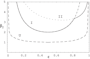
Figure 1. An illustration of the lower bound (curve I) given in Proposition 16, the lower bound (curve II) given in Proposition 8 and the $U$-shaped region for the two-star model.

4.1. Along $\epsilon=1/2$ Line

In general, we proved that there exists some critical number $\beta_{2}^{c}>0$ such that the optimizing graphon is uniform for any $0<\beta_{2}<\beta_{2}^{c}$ and non-uniform for any $\beta_{2}>\beta_{2}^{c}$. But we are far from determining the exact value of $\beta_{2}^{c}$. For very special case, the two-star model along the line $\epsilon=1/2$, we can show that $\beta_{2}^{c}=2$.

Proposition 18.

For the two-star model, along the line $\epsilon=1/2$, the optimizing graphon in (1.11) is uniform if $\beta_{2}\leq 2$ and it is not if $\beta_{2}>2$.

Proof.

First, by Proposition 16, for any $\beta_{2}>\frac{1}{2\epsilon(1-\epsilon)}=\frac{1}{2\frac{1}{2}(1-\frac{1}{2})}=2$, the optimizer is not uniform. Next, let us prove that it is uniform if $\beta_{2}\leq 2$. Let us recall from the proof of Proposition 15 that for optimal $h$, the values of $g(x)=\int_{0}^{1}h(x,y)dy$ are the roots of

$$F(z)=z-\int_{0}^{1}\frac{dy}{1+e^{2\beta_{1}-2\beta_{2}z-2\beta_{2}g(y)}}.$$ (4.9)

Differentiating with respect to $z$, we get

$$F^{\prime}(z)=1-\int_{0}^{1}\frac{2\beta_{2}e^{2\beta_{1}-2\beta_{2}z-2\beta_{2}g(y)}dy}{(1+e^{2\beta_{1}-2\beta_{2}z-2\beta_{2}g(y)})^{2}}.$$ (4.10)

It is clear $F^{\prime}(z)\geq 1>0$ if $\beta_{2}\leq 0$. Now, if $\beta_{2}>0$, since $\frac{4x}{(1+x)^{2}}\leq 1$ for any $x>0$, we have

$$F^{\prime}(z)\geq 1-\frac{\beta_{2}}{2}\geq 0,$$ (4.11)

if $\beta_{2}\leq 2$. Suppose $F^{\prime}(z)=0$, then the equality holds and we must have $2\beta_{1}-2\beta_{2}z-2\beta_{2}g(y)=0$ for a.e. $y$. Since $\beta_{2}>0$, $g(y)$ is a constant a.e. and so is $h(x,y)$. Otherwise, we have $F^{\prime}(z)>0$. When $F$ is strictly increasing, $g(x)=\int_{0}^{1}h(x,y)dy$ takes only one value, which is $1/2$ and so is $h(x,y)$ for any $x,y$. Thus when $\beta_{2}\leq 2$, the optimizer is uniform. ∎

Remark 19.

For general $p$-star model, $p\geq 2$, we can compute that for $\beta_{2}>0$,

$$F^{\prime}(z)=1-p(p-1)\beta_{2}z^{p-2}\int_{0}^{1}\frac{e^{2\beta_{1}-p\beta_{2}z^{p-1}-p\beta_{2}g^{p-1}(y)}dy}{(1+e^{2\beta_{1}-p\beta_{2}z^{p-1}-p\beta_{2}g^{p-1}(y)})^{2}}\leq 1-\frac{p(p-1)}{4}\beta_{2}.$$ (4.12)

Thus $F^{\prime}(z)\geq 0$ if $\beta_{2}\leq\frac{4}{p(p-1)}$. Similarly to the arguments in Proposition 18, we conclude that the optimizing graphon is uniform if $\beta_{2}\leq\frac{4}{p(p-1)}$. Recall that we already proved that the optimizing graphon is uniform if $(\epsilon,\frac{\beta_{2}}{2})$ is outside of the $U$-shaped region and in particular when $\epsilon=\frac{p-1}{p}$, the optimizing graphon is uniform if $\beta_{2}\leq\frac{1}{2}\frac{p^{p-1}}{(p-1)^{p}}$. It is easy to check that $\frac{4}{p(p-1)}>\frac{1}{2}\frac{p^{p-1}}{(p-1)^{p}}$ and thus provides a better bound for $p\leq 3$.

Proposition 20.

For the two-star model, along the line $\epsilon=1/2$, if $h$ is an optimizer in (1.11) then so is $1-h$.

Proof.

It is easy to check that $I(x)=I(1-x)$, $0\leq x\leq 1$ and moreover

$$\int_{0}^{1}\left(\int_{0}^{1}(1-h(x,y))dy\right)^{2}dx$$ (4.13)

$$=\int_{0}^{1}\left(\int_{0}^{1}h(x,y)dy\right)^{2}dx+1-2\int_{0}^{1}\int_{0}^{1}h(x,y)dxdy$$

$$=\int_{0}^{1}\left(\int_{0}^{1}h(x,y)dy\right)^{2}dx$$

if $\iint_{[0,1]^{2}}h(x,y)dxdy=\frac{1}{2}$. Therefore, if $h$ is an optimizer for the two-star model, so is $1-h$. ∎

Proposition 21.

For the two-star model, along the line $\epsilon=1/2$, $\beta_{2}>2$, the graphon

$$h(x,y)=\begin{cases}\frac{1}{2}+\delta(\beta_{2})&\text{if $0<x,y<\frac{1}{2}$}\\ \frac{1}{2}-\delta(\beta_{2})&\text{if $\frac{1}{2}<x,y<1$}\\ \frac{1}{2}&\text{otherwise}\end{cases}$$ (4.14)

is a stationary point in (1.11), where $\delta(\beta_{2})$ is the unique solution to the equation $\log\left(\frac{\frac{1}{2}+\delta}{\frac{1}{2}-\delta}\right)-2\beta_{2}\delta=0$ on the interval $(0,\frac{1}{2})$.

Proof.

Let us consider the graphon

$$h(x,y)=\begin{cases}\frac{1}{2}+\delta&\text{if $0<x,y<\frac{1}{2}$}\\ \frac{1}{2}-\delta&\text{if $\frac{1}{2}<x,y<1$}\\ \frac{1}{2}&\text{otherwise}\end{cases},$$ (4.15)

where $0\leq\delta<\frac{1}{2}$ is a parameter to be determined later. It is easy to check that $\iint_{[0,1]^{2}}h(x,y)dxdy=\frac{1}{2}$ and

$$g(x):=\int_{0}^{1}h(x,y)dy=\begin{cases}\frac{1}{2}+\frac{\delta}{2}&\text{if $0<x<\frac{1}{2}$}\\ \frac{1}{2}-\frac{\delta}{2}&\text{if $\frac{1}{2}<x<1$}\end{cases}.$$ (4.16)

Therefore, we have

$$2\beta_{2}-2\beta_{2}g(x)-2\beta_{2}g(y)=\log\left(\frac{1-h(x,y)}{h(x,y)}\right),\qquad 0<x,y<1,$$ (4.17)

if we let $2\beta_{2}\delta=\log\left(\frac{\frac{1}{2}+\delta}{\frac{1}{2}-\delta}\right)$. Hence, the graphon satisfies the Euler-Lagrange equation and is therefore a stationary point. For any $\beta_{2}>2$, let us define

$$G(\delta):=\log\left(\frac{\frac{1}{2}+\delta}{\frac{1}{2}-\delta}\right)-2\beta_{2}\delta.$$ (4.18)

Then, $G(0)=0$, $\lim_{\delta\uparrow\frac{1}{2}}G(\delta)=+\infty$ and

$$G^{\prime}(\delta)=\frac{1}{\frac{1}{2}-\delta}+\frac{1}{\frac{1}{2}+\delta}-2\beta_{2},\qquad G^{\prime\prime}(\delta)=\frac{1}{(\frac{1}{2}-\delta)^{2}}-\frac{1}{(\frac{1}{2}+\delta)^{2}}.$$ (4.19)

Thus, $G^{\prime\prime}(\delta)>0$ for any $0<\delta<\frac{1}{2}$ and $G^{\prime}(0)<0$ since $\beta_{2}>2$. Therefore, $G(\delta)=0$ has a unique solution on $(0,\frac{1}{2})$. ∎

Remark 22.

It would be interesting to know if the $h$ defined in (4.14) is indeed the optimizer. That does not seem to be the case. Indeed, one can show that the $h$ defined in (4.14) in Proposition 21 is a saddle point at least for $\beta_{2}>4$. Up to second variation, $\iint_{[0,1]^{2}}\delta h(x,y)dxdy=0$ and $\delta h(x,y)=\delta h(y,x)$,

$$\delta\psi =\beta_{2}\int_{0}^{1}\left(\int_{0}^{1}h(x,y)+\delta h(x,y)dy\right)^{2}dx-\beta_{2}\int_{0}^{1}\left(\int_{0}^{1}h(x,y)dy\right)^{2}dx$$ (4.20)

$$\qquad\qquad\qquad\qquad-\frac{1}{2}\iint_{[0,1]^{2}}[I(h+\delta h)-I(h)]dxdy$$

$$=2\beta_{2}\int_{0}^{1}\left(\int_{0}^{1}h(x,y)dy\right)\left(\int_{0}^{1}\delta h(x,y)dy\right)dx+\beta_{2}\int_{0}^{1}\left(\int_{0}^{1}\delta h(x,y)dy\right)^{2}dx$$

$$\qquad\qquad-\frac{1}{2}\iint_{[0,1]^{2}}I^{\prime}(h)\delta hdxdy-\frac{1}{4}\iint_{[0,1]^{2}}I^{\prime\prime}(h)(\delta h)^{2}dxdy$$

$$=\beta_{2}\int_{0}^{1}\left(\int_{0}^{1}\delta h(x,y)dy\right)^{2}dx-\frac{1}{4}\iint_{[0,1]^{2}}I^{\prime\prime}(h)(\delta h)^{2}dxdy$$

Moreover, observe that

$$I^{\prime\prime}(h)=\begin{cases}\frac{1}{\frac{1}{2}-\delta}+\frac{1}{\frac{1}{2}+\delta}&\text{if $0<x,y<\frac{1}{2}$ or $\frac{1}{2}<x,y<1$}\\ 4&\text{otherwise}\end{cases}.$$ (4.21)

Therefore, by (4.20) and (4.21), we have

$$\delta\psi =\beta_{2}\int_{0}^{1}\left(\int_{0}^{1}\delta h(x,y)dy\right)^{2}dx$$ (4.22)

$$\qquad\qquad-\frac{1}{1-4\delta^{2}}\iint_{R_{1}}(\delta h(x,y))^{2}dxdy-\iint_{R_{2}}(\delta h(x,y))^{2}dxdy$$

where

$$R_{1}:=\left\{(x,y):0<x,y<\frac{1}{2}\right\}\bigcup\left\{(x,y):\frac{1}{2}<x,y<1\right\},\quad R_{2}:=[0,1]^{2}\backslash R_{1}.$$ (4.23)

Consider $\delta h(x,y)$ defined as $\delta h(x,y)=\epsilon$ if $(x,y)\in R_{1}$ and $\delta h(x,y)=-\epsilon$ if $(x,y)\in R_{2}$. Then, $\iint_{[0,1]^{2}}\delta h(x,y)dxdy=0$ and we can compute that

$$\delta\psi=-\frac{1}{2}\left(\frac{1}{1-4\delta^{2}}+1\right)\epsilon^{2}.$$ (4.24)

On the other hand, consider $\delta h(x,y)$ defined as

$$\delta h(x,y)=\begin{cases}\epsilon&\text{if $0<x<\frac{1}{2}$,$\frac{3}{4}<y<1$ or $\frac{3}{4}<x<1$, $0<y<\frac{1}{2}$}\\ -\epsilon&\text{if $0<x<\frac{1}{2}$,$\frac{1}{2}<y<\frac{3}{4}$ or $\frac{1}{2}<x<\frac{3}{4}$, $0<y<\frac{1}{2}$}\\ 0&\text{otherwise}\end{cases}.$$ (4.25)

Then, $\iint_{[0,1]^{2}}\delta h(x,y)dxdy=0$ and we can compute that

$$\delta\psi=\frac{\beta_{2}}{2}\frac{\epsilon^{2}}{4}-\frac{\epsilon^{2}}{2}.$$ (4.26)

Hence, for $\beta_{2}>4$, $h$ defined in (4.14) is a saddle point.

4.2. Phase Transition

In Proposition 8, we showed that for a general simple subgraph $H$ satisfying the condition $e(H)>v(H)/2$, when

$$\beta_{2}>\frac{-\frac{1}{2}[\epsilon\log\epsilon+(1-\epsilon)\log(1-\epsilon)]}{\epsilon^{v(H)/2}-\epsilon^{e(H)}},$$ (4.27)

the optimizing graphon is not uniform. On the other hand, by Proposition 5, for $\beta_{2}\geq 0$, there exists a $U$-shaped region outside of which the optimizing graph is uniform. Therefore, fix the edge density $\epsilon$, if we view $\psi(\epsilon,\beta_{2})$ as a function of $\beta_{2}$, it is constant in $\beta_{2}$ on a non-trivial interval. By complex analysis, if $\psi(\epsilon,\beta_{2})$ were analytic in $\beta_{2}$, then it would be constant everywhere. Hence, for any fixed edge density $\epsilon$, there exists a positive $\beta_{2}$ at which we have non-analyticity. It is also worth mentioning that the non-analyticity in positive $\beta_{2}$ may be alternatively derived using Theorem 1.1. in [18]. This is also briefly mentioned in [10], where the non-analyticity in negative $\beta_{2}$ is proved.

5. Summary and Open Questions

We have studied the constrained exponential random graph models introduced by Kenyon and Yin [10]. We showed uniform and non-uniform structure for very general underlying graph $H$. For $\beta_{2}$ close to zero, either in the attractive regime or repulsive regime, the optimal graphon will be uniform and for $\beta_{2}$ sufficiently large, the optimal graphon will be non-uniform. It remains open to find the exact optimizing graphon structure for finite large $\beta_{2}$. It is worth mentioning that similar phenomena have been observed for the micro-canonical ensembles in Radin and Sadun [18]. They showed how the entropy changes when it is close to the so-called Erdős-Renyí density. That can give an alternative approach to giving some estimates on when the asymptotic structure for the canonical ensembles is uniform that was considered in this paper.

More results are obtained when $H$ is a $p$-star. In the case when $H$ is a two-star, we can show that along the line $\epsilon=1/2$, the asymptotic structure is uniform if $\beta_{2}\leq 2$ and is non-uniform if $\beta_{2}>2$. For general $H$, we do not have a sharp result. This remains the major challenging open problem for future investigations. Even if we cannot get a sharp result for general $H$, is it possible to show a sharp transition for a concrete model, e.g. edge-triangle model along the line $\epsilon=1/2$?

We also found and proved a stationary point for the two-star model and it remains an open question if it is indeed a local/global optimizer. Similar results should hold for the corresponding micro-canonical model. When $H$ is a $p$-star, we showed that the optimizing graphon must be multipodal. The numerical results for the corresponding micro-canonical model suggest that the optimizing graphons should indeed be bipodal, see Kenyon et al [9]. The same conjecture can be said in our case.

References

• [1] Ahlswede, R. and G. O. H. Katona. (1978). Graphs with maximal number of adjacent pairs of edges. Acta Math. Acad. Sci. Hungar. 32, 97-120.
• [2] Aristoff, D. and L. Zhu. (2014). On the phase transition curve in a directed exponential random graph model. arXiv:1404.6514.
• [3] Aristoff, D. and L. Zhu. (2015). Asymptotic structure and singularities in constrained directed graphs. Stochastic Processes and their Applications. 125, 4154-4177.
• [4] Besag, J. (1975). Statistical analysis of non-lattice data. J. R. Stat. Soc., Ser. D. Stat. 24, 179-195.
• [5] Chatterjee, S. and P. Diaconis. (2013). Estimating and understanding exponential random graph models. Annals of Statistics. 41, 2428-2461.
• [6] Chatterjee, S. and S. R. S. Varadhan. (2011). The large deviation principle for the ErdΕ‘s-RΓ©nyi random graph. European. J. Combin. 32, 1000-1017.
• [7] Fienberg, S. E. (2010). Introduction to papers on the modeling and analysis of network data. Ann. Appl. Statist. 4, 1-4.
• [8] Fienberg, S. E. (2010). Introduction to papers on the modeling and analysis of network data–II. Ann. Appl. Statist. 4, 533-534.
• [9] Kenyon, R., Radin, C., Ren K. and L. Sadun. (2014). Multipodal structure and phase transitions in large constrained graphs. arXiv:1405.0599.
• [10] Kenyon, R. and M. Yin. (2014). On the asymptotics of constrained exponential random graphs. arXiv:1406.3662.
• [11] LovΓ‘sz, L. Large Networks and Graph Limits. American Mathematical Society, Providence, 2012.
• [12] LovΓ‘sz, L. (2009). Very large graphs. Current Develop. Math. 2008, 67-128.
• [13] Newman, M. E. J. (2010). Networks: An Introduction. Oxford University Press, Oxford.
• [14] Pikhurko, O. and A. Razborov. (2017). Asymptotic structure of graphs with the minimum number of triangles. Combinatorics, Probability and Computing. 26, 138-160.
• [15] Radin, C. and M. Yin. (2013). Phase transitions in exponential random graphs. Annals of Applied Probability. 23, 2458-2471.
• [16] Radin, C. and L. Sadun. (2013). Phase transitions in a complex network. J. Phys. A: Math. Theor. 46, 305002.
• [17] Radin, C., Ren, K. and L. Sadun. (2014). The asymptotics of large constrained graphs. J. Phys. A: Math. Theor. 47, 175001.
• [18] Radin, C. and L. Sadun. (2015). Singularities in the entropy of asymptotically large simple graphs. J. Stat. Phys. 158, 853-865.
• [19] Rinaldo, A., Fienberg, S. and Y. Zhou. (2009). On the geometry of discrete exponential families with application to exponential random graph models. Electron. J. Stat. 3, 446-484.
• [20] Snijders, T. A. B., Pattison, P., Robins, G. L. and M. Handcock. (2006). New specifications for exponential random graph models. Sociological Methodology. 36, 99-153.
• [21] Wasserman, S. and K. Faust. (2010). Social Network Analysis: Methods and Applications. Structural Analysis in the Social Sciences, 2nd ed. Cambridge Univ. Press, Cambridge.
• [22] Yin, M. (2013). Critical phenomena in exponential random graphs. Journal of Statistical Physics. 153, 1008-1021.
• [23] Yin, M., Rinaldo, A. and S. Fadnavis. (2016). Asymptotic quantization of exponential random graphs. Annals of Applied Probability. 26, 3251-3285.