Multicomponent Dark Matter in Radiative Seesaw Model
and Monochromatic Neutrino Flux

Abstract

We consider a two loop radiative seesaw model with an exact $Z_{2}\times Z^{\prime}_{2}$ symmetry, which can stabilize two or three dark matter particles. The model is a simple extension of the inert scalar model of Ma, where the lepton-number violating mass term of the inert scalar, which is required to be small for small neutrino masses, is generated at the one-loop level. The semi-annihilation processes of different dark matter particles, which are present when there exist more than three different dark matter particles, not only play an important role for their relic densities but also are responsible for the monochromatic neutrino lines resulting from the dark matter annihilation processes. The monochromatic neutrinos do not suffer from a chiral suppression, and we investigate the observational possibility of the monochromatic neutrino flux from the Sun.

I Introduction

Tiny neutrino masses and the absence of dark matter (DM) candidates are problems of the standard model (SM), which can be overcome only by its extension. The tiny neutrino masses can be explained by the seesaw mechanism Minkowski:1977sc , which usually requires an introduction of right-handed neutrinos with lepton-number violating Majorana masses. However, for the tree-level seesaw mechanism to work, an undesirable hierarchy in the mass scale or in the size of the Yukawa couplings has to be introduced: To obtain neutrino masses of $\mathcal{O}(0.1)$ eV in the type I seesaw for instance, we need either large Majorana masses of Grand Unified Theory scale or very small Yukawa couplings of $\mathcal{O}(10^{-6})$ of the right-handed neutrinos with the left-handed ones if the Majorana masses are $\mathcal{O}(1)$ TeV. This unwelcome feature can be avoided if the neutrino masses are generated radiatively (Krauss:2002px -Ma:2006km for instance). With an increasing number of loops, the hierarchy between the SM scale and the Majorana masses becomes milder, and in fact the Majorana masses can become $\mathcal{O}(1)$ TeV without making the Yukawa couplings very small. The common feature of the radiative seesaw models is the existence of an unbroken discrete symmetry, which forbids the appearance of Dirac neutrino masses. An important consequence of this unbroken symmetry, usually $Z_{2}$, is that the lightest $Z_{2}$ odd particle is stable and hence can be a DM candidate with a mass of $\mathcal{O}(1)$ TeV.

In the one-loop radiative seesaw model of Ma Ma:2006km , the lepton-number violating mass term of the inert doublet scalar $\eta$ is required to be very small to obtain small neutrino masses. The mass term originates from a lepton-number violating quartic scalar coupling, the ”$\lambda_{5}$ coupling”, which is $\mathcal{O}(10^{-5})$ to obtain small neutrino masses with the Yukawa couplings of $\mathcal{O}(0.01)$. In this paper, we consider an extension of the model such that this lepton-number violating mass, too, is generated radiatively. Consequently, the seesaw mechanism occurs at the two-loop level in the extended model Aoki:2013gzs (A similar idea has been proposed in an $E_{6}$ inspired model Ma:2007yx .) . For this mechanism to work, we have to introduce a larger unbroken discrete symmetry, $Z_{2}\times Z_{2}$, which implies that the model yields a multicomponent DM system Ma:2007yx -Aoki:2012ub . We emphasize that the multicomponent DM system is a consequence of the unbroken $Z_{2}\times Z_{2}$, which forbids the Dirac neutrino masses and also the one-loop neutrino mass diagram.

In Aoki:2013gzs we have investigated in the extended model the two-component DM system consisting of a neutral component of $\eta$ and another real scalar $\chi$. We have found that the $\chi$ DM can cover the shortage of the relic density of the $\eta$ DM for the mass range 100 GeV $\lesssim m_{\eta}\lesssim$ 600 GeV Barbieri:2006dq ; LopezHonorez:2006gr . We were motivated by the desire to explain at the same time a slight excess of the Higgs decay into two $\gamma$’s :2012gk and the $135$ GeV $\gamma$-ray line possibly observed at the Fermi LAT Ackermann:2012qk by the annihilation of the $\chi$ DM. Though it is not impossible to explain both $\gamma$ excesses, we have to use a corner of the parameter space, which faces the border of perturbation theory. Moreover, the subsequent experimental searches could not confirm these interesting $\gamma$ excesses ATLAS:2013mma ; Gustafsson:2013fca .

In this paper we consider the same model in the parameter space leading to a three-component DM system: Our DM candidates are the lightest right-handed neutrino $N$, and two real scalars $\phi_{R}$ and $\chi$. The semi-annihilation processes of these DM particles have a considerable influence on their relic densities Aoki:2012ub ; D'Eramo:2010ep , and the monochromatic neutrino lines can be produced from the semi-annihilation process such as $\phi_{R}\chi\to N\nu$. These monochromatic neutrinos are not chirally suppressed, and we analyze the observational prospect of the monochromatic neutrino flux from the Sun. Semi-annihilations of DM particles can produce line spectra of neutral SM particles, e.g. neutrinos Aoki:2012ub and photons D'Eramo:2012rr , and observations of such line spectra are indications of a multicomponent DM Universe .

II Model

Table 1: The matter contents of the model and the corresponding quantum numbers. $Z_{2}\times Z^{\prime}_{2}$ is the unbroken discrete symmetry, while the lepton number $L$ is softly broken by the $\phi$ mass.

field	statistics	$SU(2)_{L}$	$U(1)_{Y}$	$Z_{2}$	$Z^{\prime}_{2}$	$L$
$(\nu_{L},l_{L})$	F	$2$	$-1/2$	$+$	$+$	$1$
$l^{c}_{R}$	F	$1$	$1$	$+$	$+$	$-1$
$N^{c}_{R}$	F	$1$	$0$	$-$	$+$	$0$
$H=(H^{+},H^{0})$	B	$2$	$1/2$	$+$	$+$	$0$
$\eta=(\eta^{+},\eta^{0})$	B	$2$	$1/2$	$-$	$+$	$-1$
$\chi$	B	$1$	$0$	$+$	$-$	$0$
$\phi$	B	$1$	$0$	$-$	$-$	$1$

Here we will briefly outline the model Aoki:2013gzs , where we show the matter content of the model in Table I. In addition to the matter content of the SM model, we introduce the right-handed neutrino $N_{R}^{c}$, an $SU(2)_{L}$ doublet scalar $\eta$, and two SM singlet scalars $\chi$ and $\phi$. Note that the lepton number $L$ of $N_{R}^{c}$ is zero. The $Z_{2}\times Z^{\prime}_{2}\times L$ -invariant Yukawa sector and Majorana mass term for $N_{R}^{c}$ can be described by

$$\mathcal{L}_{Y}=Y^{e}_{ij}H^{\dagger}L_{i}l_{Rj}^{c}+Y^{\nu}_{ik}L_{i}\epsilon\eta N_{Rk}^{c}-\frac{1}{2}M_{k}N_{Rk}^{c}N_{Rk}^{c}+h.c.~{},$$ (1)

where $i,j,k~{}(=1,2,3)$ stand for the flavor indices. The scalar potential $V$ is written as $V=V_{\lambda}+V_{m}$, where

$$V_{\lambda} = \lambda_{1}(H^{\dagger}H)^{2}+\lambda_{2}(\eta^{\dagger}\eta)^{2}+\lambda_{3}(H^{\dagger}H)(\eta^{\dagger}\eta)+\lambda_{4}(H^{\dagger}\eta)(\eta^{\dagger}H)$$ (2)

$$+\gamma_{1}\chi^{4}+\gamma_{2}(H^{\dagger}H)\chi^{2}+\gamma_{3}(\eta^{\dagger}\eta)\chi^{2}+\gamma_{4}|\phi|^{4}+\gamma_{5}(H^{\dagger}H)|\phi|^{2}$$

$$+\gamma_{6}(\eta^{\dagger}\eta)|\phi|^{2}+\gamma_{7}\chi^{2}|\phi|^{2}+\frac{\kappa}{2}[\,(H^{\dagger}\eta)\chi\phi+h.c.\,]~{},$$

$$V_{m} = m_{1}^{2}H^{\dagger}H+m_{2}^{2}\eta^{\dagger}\eta+\frac{1}{2}m_{3}^{2}\chi^{2}+m_{4}^{2}|\phi|^{2}+\frac{1}{2}m_{5}^{2}[\,\phi^{2}+(\phi^{*})^{2}\,]~{}.$$ (3)

The potential $V$, except the last term in $V_{m}$, is $Z_{2}\times Z^{\prime}_{2}\times L$ -invariant. This last term breaks the lepton number softly. In the absence of this term, there will be no neutrino mass. Note that the “$\lambda_{5}$ term”, $(1/2)\lambda_{5}(H^{\dagger}\eta)^{2}$, is also forbidden by $L$. A small $\lambda_{5}$ of the original model of Ma Ma:2006km is “natural” according to ’t Hooft 'tHooft:1979bh , because the absence of $\lambda_{5}$ implies an enhancement of symmetry. In fact, if $\lambda_{5}$ is small at some scale, it remains small for other scales as one can explicitly verify Bouchand:2012dx . Here we attempt to derive the smallness of $\lambda_{5}$ dynamically, such that the $\lambda_{5}$ term becomes calculable.

The charged, CP even and odd scalars are defined as

$$H = \left(\begin{array}[]{c}H^{+}\\ (v_{h}+h+iG)/\sqrt{2}\\ \end{array}\right)~{},~{}\eta=\left(\begin{array}[]{c}\eta^{+}\\ (\eta_{R}^{0}+i\eta_{I}^{0})/\sqrt{2}\\ \end{array}\right)~{},~{}\phi=(\phi_{R}+i\phi_{I})/\sqrt{2}~{},$$ (8)

where $v_{h}$ is the vacuum expectation value. The tree-level masses of the scalars are given by

$$m_{h}^{2} =2\lambda_{1}v_{h}^{2}~{},$$ (9)

$$m^{2}_{\eta^{\pm}} =m_{2}^{2}+\frac{1}{2}\lambda_{3}v_{h}^{2}~{},~{}m^{2}_{\eta_{R}^{0}}=m^{2}_{\eta_{I}^{0}}=m_{2}^{2}+\frac{1}{2}(\lambda_{3}+\lambda_{4})v_{h}^{2}~{},$$ (10)

$$m^{2}_{\phi_{R}} =m_{4}^{2}+m_{5}^{2}+\gamma_{5}v_{h}^{2}~{},~{}m^{2}_{\phi_{I}}=m_{4}^{2}-m_{5}^{2}+\gamma_{5}v_{h}^{2}~{},$$ (11)

$$m^{2}_{\chi} =m_{3}^{2}+\gamma_{2}v_{h}^{2}~{}.$$ (12)

As we see from (10), the tree-level mass of $\eta^{0}_{R}$ is the same as that of $\eta^{0}_{I}$. At the one-loop level, this degeneracy is lifted because the $\lambda_{5}$ term is generated at this order:

$$\lambda_{5}^{\rm eff} = -\frac{\kappa^{2}}{64\pi^{2}}\left[\frac{m^{2}_{\phi_{I}}}{m^{2}_{\phi_{I}}-m_{\chi}^{2}}\ln\frac{m^{2}_{\phi_{I}}}{m_{\chi}^{2}}-\frac{m^{2}_{\phi_{R}}}{m^{2}_{\phi_{R}}-m_{\chi}^{2}}\ln\frac{m^{2}_{\phi_{R}}}{m_{\chi}^{2}}\right]$$ (13)

$$\sim -\frac{\kappa^{2}}{64\pi^{2}}\frac{m_{5}^{2}}{m_{\phi_{R}}^{2}-m_{\chi}^{2}}\left[1-\frac{m^{2}_{\chi}}{m^{2}_{\phi_{R}}-m_{\chi}^{2}}\ln\frac{m^{2}_{\phi_{R}}}{m_{\chi}^{2}}\right]~{}\mbox{for}~{}m_{5}\ll m_{\phi_{R}}~{}.$$

In other words the origin of this correction is the one-loop self-energy diagram that can be embedded into the two-loop diagram to generate the neutrino mass (see Fig. 1):

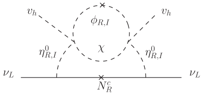
Figure 1: The two-loop diagram that is responsible for the radiative generation of the neutrino mass. The one-loop self-energy diagram inside of this two-loop diagram is the origin of the mass difference between $m_{\eta_{R}^{0}}$ and $m_{\eta_{I}^{0}}$ as well as the effective coupling $\lambda^{\rm eff}_{5}$ in Eq. (13).

$$({\cal M}_{\nu})_{ij} = \frac{Y^{\nu}_{ik}Y^{\nu}_{jk}}{16(4\pi)^{4}}\kappa^{2}v_{h}^{2}M_{k}(m_{\phi_{I}}^{2}-m_{\phi_{R}}^{2})\int_{0}^{1}dx_{1}\int_{0}^{1-x_{1}}dx_{2}\int_{0}^{1}dy\left(\frac{y}{\beta-(x_{1}-x_{1}^{2})M_{k}^{2}}\right)$$ (14)

$$\times\left[\frac{x_{1}-x_{1}^{2}}{(1-y)\beta+y(x_{1}-x_{1}^{2})m_{\eta^{0}}^{2}}-\frac{1}{(1-y)M_{k}^{2}+ym_{\eta^{0}}^{2}}\right]~{},$$

where $\beta\equiv m_{\phi_{I}}^{2}+x_{1}(m_{\chi}^{2}-m_{\phi_{R}}^{2})+x_{2}(m_{\phi_{I}}^{2}-m_{\phi_{R}}^{2})$, and we have assumed that $m_{\eta^{0}}=m_{\eta_{R}^{0}}\simeq m_{\eta_{I}^{0}}$. Using $\lambda_{5}^{\rm eff}$ given in (13), the neutrino mass matrix can be approximated as

$$({\cal M}_{\nu})_{ij} = -\frac{\lambda_{5}^{\rm eff}v_{h}^{2}}{8\pi^{2}}\sum_{k}\frac{Y^{\nu}_{ik}Y^{\nu}_{jk}M_{k}}{m_{\eta^{0}}^{2}-M_{k}^{2}}\left[1-\frac{M_{k}^{2}}{m_{\eta^{0}}^{2}-M_{k}^{2}}\ln\frac{m_{\eta^{0}}^{2}}{M_{k}^{2}}\right].$$ (15)

We see from (14) that the neutrino mass matrix ${\cal M}_{\nu}$ is proportional to $|Y^{\nu}\kappa|^{2}m_{5}^{2}$ (because $(m_{\phi_{R}}^{2}-m_{\phi_{I}}^{2})=2m^{2}_{5}$). Therefore, only this combination for a given set of $m_{\chi}~{},~{}m_{\phi_{R}}~{},~{}m_{\eta_{0}}$ and $M_{k}$ can be fixed by the neutrino mass: $m_{\chi}$, $m_{\phi_{R}}$, $m_{\eta^{0}}$, $M_{k}\sim\mathcal{O}(10^{2})~{}\mathrm{GeV}$, for instance, implies that $|Y^{\nu}\kappa|m_{5}\sim\mathcal{O}(10^{-2})~{}\mathrm{GeV}$ to obtain the neutrino mass scale of $\mathcal{O}(0.1)~{}\mathrm{eV}$. With the same set of the parameter values we find that $\lambda^{\rm eff}_{5}\sim 10^{-4}$, where the smallness $\lambda^{\rm eff}_{5}$ is a consequence of the radiative generation of this coupling. As we will see, the product $|Y^{\nu}\kappa|$ enters into the semi-annihilation of DM particles that produces monochromatic neutrinos, while the upper bound of $|Y^{\nu}|$ follows from the $\mu\to e\gamma$ constraint.

II.1 The stability of the scalar potential and the perturbativity constraint

If the parameters of the scalar potential $V=V_{\lambda}+V_{m}$ satisfy the following conditions, the potential is bounded from below and the DM stabilizing symmetry $Z_{2}\times Z^{\prime}_{2}$ remains unbroken at the tree-level:

$$m_{1}^{2}<0~{},~{}~{}m_{2}^{2}>0~{},~{}~{}m_{3}^{2}>0~{},~{}~{}m_{4}^{2}>0~{},~{}~{}|m_{5}^{2}|<m_{4}^{2}~{},~{}$$

$$\lambda_{1}>0~{},~{}~{}\lambda_{2}>0~{},~{}~{}\gamma_{1}>0~{},~{}~{}\gamma_{4}>0~{},~{}$$

$$\lambda_{3}>-\frac{2}{3}\sqrt{\lambda_{1}\lambda_{2}}~{},~{}~{}\lambda_{3}+\lambda_{4}>-\frac{2}{3}\sqrt{\lambda_{1}\lambda_{2}}~{},~{}$$

$$\gamma_{2}>-\frac{2}{3}\sqrt{\lambda_{1}\gamma_{1}}~{},~{}~{}\gamma_{3}>-\frac{2}{3}\sqrt{\lambda_{2}\gamma_{1}}~{},~{}~{}\gamma_{5}>-\frac{2}{3}\sqrt{\lambda_{1}\gamma_{4}}~{},~{}$$

$$\gamma_{6}>-\frac{2}{3}\sqrt{\lambda_{2}\gamma_{4}}~{},~{}~{}\gamma_{7}>-\frac{2}{3}\sqrt{\gamma_{1}\gamma_{4}}~{},~{}$$ (16)

$$|\kappa|<\lambda_{1}+\lambda_{2}+\gamma_{1}+\gamma_{4}-\frac{2}{3}\left(\sqrt{\lambda_{1}\lambda_{2}}+\sqrt{\lambda_{1}\gamma_{1}}+\sqrt{\lambda_{1}\gamma_{4}}+\sqrt{\lambda_{2}\gamma_{1}}+\sqrt{\lambda_{2}\gamma_{4}}+\sqrt{\gamma_{1}\gamma_{4}}\right)~{}.$$

We further assume that $|\lambda_{i}|$, $|\gamma_{i}|$, $|\kappa|$ $<1$ ensures the perturbativeness of the model. Under these assumptions, it is noted that the above stability conditions give $|\kappa|\lesssim 0.4$.

II.2 $\mu\rightarrow e\gamma$ constraint

The strongest constraint on $Y^{\nu}$ comes from $\mu\to e\gamma$ , which is given by Ma:2001mr ; Adam:2013mnn

$$B(\mu\rightarrow e\gamma)={3\alpha\over 64\pi(G_{F}m_{\eta^{\pm}}^{2})^{2}}\left|~{}\sum_{k}Y^{\nu}_{\mu k}Y^{\nu}_{ek}F_{2}\left({M_{k}^{2}\over m_{\eta^{\pm}}^{2}}\right)\right|^{2}\mathrel{\mathchoice{\vbox{\offinterlineskip\halign{$\m@th\displaystyle\hfil#\hfil$\cr<\crcr\sim\crcr} }}{\vbox{\offinterlineskip\halign{$\m@th\textstyle\hfil#\hfil$\cr<\crcr\sim\crcr} }}{\vbox{\offinterlineskip\halign{$\m@th\scriptstyle\hfil#\hfil$\cr<\crcr\sim\crcr} }}{\vbox{\offinterlineskip\halign{$\m@th\scriptscriptstyle\hfil#\hfil$\cr<\crcr\sim\crcr} }}}5.7\times 10^{-13}~{},$$ (25)

$$F_{2}(x)={1\over 6(1-x)^{4}}(1-6x+3x^{2}+2x^{3}-6x^{2}\ln x)~{}.$$

A similar, but slightly weaker bound for $\tau\to\mu(e)\gamma$ given in Hayasaka:2010et has to be satisfied, too. Since $F_{2}(x)\sim 1/3x$ for $x\gg 1$, while $1/12<F_{2}(x)<1/6$ for $0<x<1$, the constraint can be readily satisfied if $M_{k}\gg m_{\eta^{\pm}}$ or $M_{k}<m_{\eta^{\pm}}$. If we assume that $M_{k}\sim m_{\eta^{\pm}}\sim\mathcal{O}(10^{2})~{}\mbox{GeV}$ in (25), the constraint (25) becomes $B(\mu\rightarrow e\gamma)\simeq 10^{-4}\times|\sum_{k}Y^{\nu}_{\mu k}Y^{\nu}_{ek}|^{2}\mathrel{\mathchoice{\vbox{\offinterlineskip\halign{$\m@th\displaystyle\hfil#\hfil$\cr<\crcr\sim\crcr} }}{\vbox{\offinterlineskip\halign{$\m@th\textstyle\hfil#\hfil$\cr<\crcr\sim\crcr} }}{\vbox{\offinterlineskip\halign{$\m@th\scriptstyle\hfil#\hfil$\cr<\crcr\sim\crcr} }}{\vbox{\offinterlineskip\halign{$\m@th\scriptscriptstyle\hfil#\hfil$\cr<\crcr\sim\crcr} }}}5.7\times 10^{-13}$. Therefore, $|Y^{\nu}_{ek}Y^{\nu}_{\mu k}|^{2}\mathrel{\mathchoice{\vbox{\offinterlineskip\halign{$\m@th\displaystyle\hfil#\hfil$\cr<\crcr\sim\crcr} }}{\vbox{\offinterlineskip\halign{$\m@th\textstyle\hfil#\hfil$\cr<\crcr\sim\crcr} }}{\vbox{\offinterlineskip\halign{$\m@th\scriptstyle\hfil#\hfil$\cr<\crcr\sim\crcr} }}{\vbox{\offinterlineskip\halign{$\m@th\scriptscriptstyle\hfil#\hfil$\cr<\crcr\sim\crcr} }}}\mathcal{O}(10^{-8})$ can satisfy the constraint.

II.3 The $T$ parameter constraint

Of the $S,T$ and $U$ parameters from the electroweak precision measurements the $T$ parameter constraint is the severest for the present model Barbieri:2006dq ; Beringer:1900zz ; Ciuchini:2013pca ,

$$\Delta T \simeq 1.08\left(\frac{m_{\eta^{\pm}}-m_{\eta^{0}_{R}}}{v_{h}}\right)\left(\frac{m_{\eta^{\pm}}-m_{\eta^{0}_{I}}}{v_{h}}\right)=0.10\pm 0.08$$ (26)

for $m_{h}=125.6\pm 0.3$ GeV. Therefore, $|m_{\eta^{\pm}}-m_{\eta^{0}_{R}}|~{},~{}|m_{\eta^{\pm}}-m_{\eta^{0}_{I}}|\mathrel{\mathchoice{\vbox{\offinterlineskip\halign{$\m@th\displaystyle\hfil#\hfil$\cr<\crcr\sim\crcr} }}{\vbox{\offinterlineskip\halign{$\m@th\textstyle\hfil#\hfil$\cr<\crcr\sim\crcr} }}{\vbox{\offinterlineskip\halign{$\m@th\scriptstyle\hfil#\hfil$\cr<\crcr\sim\crcr} }}{\vbox{\offinterlineskip\halign{$\m@th\scriptscriptstyle\hfil#\hfil$\cr<\crcr\sim\crcr} }}}90~{}\mbox{GeV}$ is sufficient to meet the requirement.

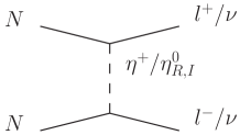
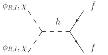
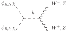
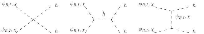
Figure 2: The diagrams for the standard annihilation processes.

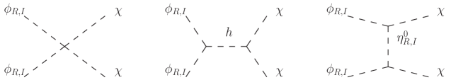
Figure 3: The diagrams for the DM conversion processes.

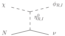
Figure 4: The diagrams for the semi-annihilation process.

III Multicomponent dark matter system

In this model there are three types of dark matter candidates $N=N^{c}_{R1}$ (the lightest among $N^{c}_{Rk}$’s) or $\eta^{0}_{R}$ (or $\eta^{0}_{I}$) with $(Z_{2},Z^{\prime}_{2})=(-,+)$, $\chi$ with $(Z_{2},Z^{\prime}_{2})=(+,-)$ and $\phi_{R}$ (or $\phi_{I}$) with $(Z_{2},Z^{\prime}_{2})=(-,-)$. For $(Z_{2},Z^{\prime}_{2})=(-,+)$ there are two candidates, and in the following discussions we assume that $N$ is a DM candidate . Therefore, our system consists of three DM particles, $N,~{}\phi_{R},~{}\chi$. Consequently, there are three types of DM annihilation process Aoki:2012ub (Figures 2-4);

$$\mathrm{Standard~{}annihilation:} ~{}NN\rightarrow XX^{\prime},~{}~{}\phi_{R}\phi_{R}\rightarrow XX^{\prime},~{}~{}\chi\chi\rightarrow XX^{\prime},~{}~{}(X,X^{\prime}\mathrm{:SM~{}particles}),~{}$$ (27)

$$\mathrm{DM~{}conversion:} ~{}\phi_{R}\phi_{R}\rightarrow\chi\chi,~{}$$ (28)

$$\mathrm{Semi}\rm{\mathchar 45\relax annihilation:} ~{}N\phi_{R}\rightarrow\chi\nu,~{}~{}\chi N\rightarrow\phi_{R}\nu,~{}~{}\phi_{R}\chi\rightarrow N\nu,~{}$$ (29)

where we assume $m_{\phi_{R}}>m_{\chi}$. Moreover, since the mass difference between $\phi_{R}$ and $\phi_{I}$ is controlled by the lepton-number breaking mass $m_{5}$, which is assumed to be much smaller than $m_{\phi_{R}}$ so that $m_{\phi_{R}}$ and $m_{\phi_{I}}$ are practically degenerate, the contribution of $\phi_{I}$ to the annihilation processes during the decoupling of DMs is non-negligible. The annihilation processes of $\phi_{I}$ are $\phi_{I}\phi_{I}\rightarrow XX^{\prime}$ (standard annihilation),  $\phi_{I}\phi_{I}\rightarrow\phi_{R}\phi_{R}$ and $\phi_{I}\phi_{I}\rightarrow\chi\chi$ (DM conversion), $N\phi_{I}\rightarrow\chi\nu,~{}\chi N\rightarrow\phi_{I}\nu$ and $\phi_{I}\chi\rightarrow N\nu~{}$ (semi-annihilation), where we have assumed that the decay of $\phi_{I}\rightarrow N\chi$ is kinematically forbidden. There is a conversion between $\phi_{R}$ and $\phi_{I}$, and its main process is shown in Fig. 5. This process is loop suppressed, and the cross section

$$\sigma_{\phi_{I}X\rightarrow\phi_{R}X^{\prime}}|v|\sim 10^{-14}\times\left(\frac{v_{h}}{246~{}\mathrm{GeV}}\right)^{4}\left(\frac{m_{\phi}}{100~{}\mathrm{GeV}}\right)^{2}\left(\frac{(100~{}\mathrm{GeV})^{6}}{m_{\eta^{0}_{R}}^{2}m_{\eta^{0}_{I}}^{2}m_{\chi}^{2}}\right)~{}\mathrm{GeV}^{-2}~{}$$ (30)

would be roughly 2 orders of magnitude smaller than that of tree-level processes. The reaction rate of this process is $\langle\sigma_{\phi_{I}X\rightarrow\phi_{R}X^{\prime}}|v|\rangle n_{\phi_{I}}n_{X}$ which is roughly $n_{\phi_{I}}^{-1}\sim\exp(m_{\phi_{I}}/T)$ times larger than the standard annihilation. Thus, during the decoupling of DMs, the reaction between $\phi_{I}$ and $\phi_{R}$ can reach chemical equilibrium, implying that

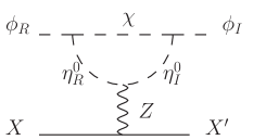
Figure 5: Conversion process between $\phi_{I}$ and $\phi_{R}$. Here $X$ and $X^{\prime}$ are SM particles.

we can use a similar method as Griest:1990kh and sum up the number densities of particles having the same $Z_{2}\times Z^{\prime}_{2}$ parities. The Boltzmann equations of their number densities $n_{N},~{}n_{\phi}\equiv n_{\phi_{I}}+n_{\phi_{R}},~{}n_{\chi}$ are given by

$$\dot{n}_{N}+3Hn_{N}= -\Bigl{\{}\langle\sigma_{NN\rightarrow XX^{\prime}}|v|\rangle(n_{N}^{2}-\bar{n}_{N}^{2})$$

$$+\langle\sigma_{N\phi\rightarrow\chi\nu}|v|\rangle(n_{N}n_{\phi}-\bar{n}_{N}\bar{n}_{\phi}\frac{n_{\chi}}{\bar{n}_{\chi}})+\langle\sigma_{N\chi\rightarrow\phi\nu}|v|\rangle(n_{N}n_{\chi}-\bar{n}_{N}\bar{n}_{\chi}\frac{n_{\phi}}{\bar{n}_{\phi}})$$

$$-\langle\sigma_{\phi\chi\rightarrow N\nu}|v|\rangle(n_{\phi}n_{\chi}-\bar{n}_{\phi}\bar{n}_{\chi}\frac{n_{N}}{\bar{n}_{N}})\Bigr{\}}~{},$$ (31)

$$\dot{n}_{\phi}+3Hn_{\phi}= -\Bigl{\{}\langle\sigma_{\phi\phi\rightarrow XX^{\prime}}|v|\rangle(n_{\phi}^{2}-\bar{n}_{\phi}^{2})+\langle\sigma_{\phi\phi\rightarrow\chi\chi}|v|\rangle(n_{\phi}^{2}-\bar{n}_{\phi}^{2}\frac{n_{\chi}^{2}}{\bar{n}_{\chi}^{2}})$$

$$+\langle\sigma_{N\phi\rightarrow\chi\nu}|v|\rangle(n_{N}n_{\phi}-\bar{n}_{N}\bar{n}_{\phi}\frac{n_{\chi}}{\bar{n}_{\chi}})-\langle\sigma_{N\chi\rightarrow\phi\nu}|v|\rangle(n_{N}n_{\chi}-\bar{n}_{N}\bar{n}_{\chi}\frac{n_{\phi}}{\bar{n}_{\phi}})$$

$$+\langle\sigma_{\phi\chi\rightarrow N\nu}|v|\rangle(n_{\phi}n_{\chi}-\bar{n}_{\phi}\bar{n}_{\chi}\frac{n_{N}}{\bar{n}_{N}})\Bigr{\}}~{},$$ (32)

$$\dot{n}_{\chi}+3Hn_{\chi}= -\Bigl{\{}\langle\sigma_{\chi\chi\rightarrow XX^{\prime}}|v|\rangle(n_{\chi}^{2}-\bar{n}_{\chi}^{2})-\langle\sigma_{\phi\phi\rightarrow\chi\chi}|v|\rangle(n_{\phi}^{2}-\bar{n}_{\phi}^{2}\frac{n_{\chi}^{2}}{\bar{n}_{\chi}^{2}})$$

$$-\langle\sigma_{N\phi\rightarrow\chi\nu}|v|\rangle(n_{N}n_{\phi}-\bar{n}_{N}\bar{n}_{\phi}\frac{n_{\chi}}{\bar{n}_{\chi}})+\langle\sigma_{N\chi\rightarrow\phi\nu}|v|\rangle(n_{N}n_{\chi}-\bar{n}_{N}\bar{n}_{\chi}\frac{n_{\phi}}{\bar{n}_{\phi}})$$

$$+\langle\sigma_{\phi\chi\rightarrow N\nu}|v|\rangle(n_{\phi}n_{\chi}-\bar{n}_{\phi}\bar{n}_{\chi}\frac{n_{N}}{\bar{n}_{N}})\Bigr{\}}~{},$$ (33)

where $H$ is the Hubble parameter. We have made approximations given by

$$\langle\sigma_{\phi\phi\rightarrow XX^{\prime}}|v|\rangle =\langle\sigma_{\phi_{I}\phi_{I}\rightarrow XX^{\prime}}|v|\rangle\frac{\bar{n}_{\phi_{I}}^{2}}{\bar{n}_{\phi}^{2}}+\langle\sigma_{\phi_{R}\phi_{R}\rightarrow XX^{\prime}}|v|\rangle\frac{\bar{n}_{\phi_{R}}^{2}}{\bar{n}_{\phi}^{2}}~{},$$ (34)

$$\langle\sigma_{\phi\phi\rightarrow\chi\chi}|v|\rangle =\langle\sigma_{\phi_{I}\phi_{I}\rightarrow\chi\chi}|v|\rangle\frac{\bar{n}_{\phi_{I}}^{2}}{\bar{n}_{\phi}^{2}}+\langle\sigma_{\phi_{R}\phi_{R}\rightarrow\chi\chi}|v|\rangle\frac{\bar{n}_{\phi_{R}}^{2}}{\bar{n}_{\phi}^{2}}~{},$$ (35)

$$\langle\sigma_{N\phi\rightarrow\chi\nu}|v|\rangle =\langle\sigma_{N\phi_{I}\rightarrow\chi\nu}|v|\rangle\frac{\bar{n}_{\phi_{I}}}{\bar{n}_{\phi}}+\langle\sigma_{N\phi_{R}\rightarrow\chi\nu}|v|\rangle\frac{\bar{n}_{\phi_{R}}}{\bar{n}_{\phi}}~{},$$ (36)

$$\langle\sigma_{N\chi\rightarrow\phi\nu}|v|\rangle =\langle\sigma_{N\chi\rightarrow\phi_{I}\nu}|v|\rangle+\langle\sigma_{N\chi\rightarrow\phi_{R}\nu}|v|\rangle~{},$$ (37)

$$\langle\sigma_{\phi\chi\rightarrow N\nu}|v|\rangle =\langle\sigma_{\phi_{R}\chi\rightarrow N\nu}|v|\rangle\frac{\bar{n}_{\phi_{R}}}{\bar{n}_{\phi}}+\langle\sigma_{\phi_{I}\chi\rightarrow N\nu}|v|\rangle\frac{\bar{n}_{\phi_{I}}}{\bar{n}_{\phi}}~{}.$$ (38)

As usual we rewrite (31), (32) and (33) for $Y_{i}\equiv n_{i}/s$, where $s$ is the entropy density. To this end, we introduce the reaction rates

$$\Gamma_{ii\rightarrow XX^{\prime}} =\langle\sigma_{ii\rightarrow XX^{\prime}}|v|\rangle\bar{n}_{i}~{},$$ (39)

$$\Gamma^{(i)}_{jj\rightarrow kk} =\langle\sigma_{jj\rightarrow kk}|v|\rangle\frac{\bar{n}_{j}^{2}}{\bar{n}_{i}}~{}~{}(\mathrm{for}~{}i=j~{}\mathrm{or}~{}k,m_{j}>m_{k})~{},$$ (40)

$$\Gamma^{(i)}_{jk\rightarrow lX} =\langle\sigma_{jk\rightarrow lX}|v|\rangle\frac{\bar{n}_{j}\bar{n}_{k}}{\bar{n}_{i}}~{}~{}(\mathrm{for}~{}i=j,~{}k~{}\mathrm{or}~{}l)~{}.$$ (41)

For $i=j=\phi$, $k=\chi$, for instance, the DM conversion rate is $\Gamma^{(\phi)}_{\phi\phi\rightarrow\chi\chi}$, while is $\Gamma^{(\chi)}_{\phi\phi\rightarrow\chi\chi}$ for $i=k=\chi$, $j=\phi$. The ratio between $\Gamma^{(\chi)}_{\phi\phi\rightarrow\chi\chi}$ and $\Gamma^{(\phi)}_{\phi\phi\rightarrow\chi\chi}$ is given by the factor $\bar{n}_{\phi}/\bar{n}_{\chi}$, which is small because $m_{\phi}>m_{\chi}$. Similarly, the ratio of the semi-annihilation process and the standard annihilation for the DM $i$ is proportional to ${\bar{n}_{j}\bar{n}_{k}}/{\bar{n}_{i}^{2}}\sim\exp(-(m_{j}+m_{k}-2m_{i})/T)=\exp(\pm(m_{j}-m_{k})/T)$ for $i=j$ or $k$. If the $\langle\sigma|v|\rangle$’s are the same order of magnitude, this factor implies a larger rate in the Boltzmann equations for the heavier DM and a smaller rate for lighter DM. In the case $i=l$, the factor is ${\bar{n}_{j}\bar{n}_{k}}/{\bar{n}_{i}^{2}}\sim\exp(-(m_{j}+m_{k}-2m_{l})/T)$ and it can be enhanced when $(m_{j}+m_{k})/2<m_{l}$. Using these reaction rates we find

$$\frac{x}{\bar{Y}_{N}}\frac{dY_{N}}{dx}= -\frac{\Gamma_{NN\rightarrow XX^{\prime}}}{H(x)}\left(\frac{Y_{N}^{2}}{\bar{Y}_{N}^{2}}-1\right)-\frac{\Gamma^{(N)}_{N\phi\rightarrow\chi\nu}}{H(x)}\left(\frac{Y_{N}Y_{\phi}}{\bar{Y}_{N}\bar{Y}_{\phi}}-\frac{Y_{\chi}}{\bar{Y}_{\chi}}\right)$$

$$-\frac{\Gamma^{(N)}_{N\chi\rightarrow\phi\nu}}{H(x)}\left(\frac{Y_{N}Y_{\chi}}{\bar{Y}_{N}\bar{Y}_{\chi}}-\frac{Y_{\phi}}{\bar{Y}_{\phi}}\right)+\frac{\Gamma^{(N)}_{\phi\chi\rightarrow N\nu}}{H(x)}\left(\frac{Y_{\phi}Y_{\chi}}{\bar{Y}_{\phi}\bar{Y}_{\chi}}-\frac{Y_{N}}{\bar{Y}_{N}}\right)~{},$$ (42)

$$\frac{x}{\bar{Y}_{\phi}}\frac{dY_{\phi}}{dx}= -\frac{\Gamma_{\phi\phi\rightarrow XX^{\prime}}}{H(x)}\left(\frac{Y_{\phi}^{2}}{\bar{Y}_{\phi}^{2}}-1\right)-\frac{\Gamma^{(\phi)}_{\phi\phi\rightarrow\chi\chi}}{H(x)}\left(\frac{Y_{\phi}^{2}}{\bar{Y}_{\phi}^{2}}-\frac{Y_{\chi}^{2}}{\bar{Y}_{\chi}^{2}}\right)-\frac{\Gamma^{(\phi)}_{N\phi\rightarrow\chi\nu}}{H(x)}\left(\frac{Y_{N}Y_{\phi}}{\bar{Y}_{N}\bar{Y}_{\phi}}-\frac{Y_{\chi}}{\bar{Y}_{\chi}}\right)$$

$$+\frac{\Gamma^{(\phi)}_{N\chi\rightarrow\phi\nu}}{H(x)}\left(\frac{Y_{N}Y_{\chi}}{\bar{Y}_{N}\bar{Y}_{\chi}}-\frac{Y_{\phi}}{\bar{Y}_{\phi}}\right)-\frac{\Gamma^{(\phi)}_{\phi\chi\rightarrow N\nu}}{H(x)}\left(\frac{Y_{\phi}Y_{\chi}}{\bar{Y}_{\phi}\bar{Y}_{\chi}}-\frac{Y_{N}}{\bar{Y}_{N}}\right)~{},$$ (43)

$$\frac{x}{\bar{Y}_{\chi}}\frac{dY_{\chi}}{dx}= -\frac{\Gamma_{\chi\chi\rightarrow XX^{\prime}}}{H(x)}\left(\frac{Y_{\chi}^{2}}{\bar{Y}_{\chi}^{2}}-1\right)+\frac{\Gamma^{(\chi)}_{\phi\phi\rightarrow\chi\chi}}{H(x)}\left(\frac{Y_{\phi}^{2}}{\bar{Y}_{\phi}^{2}}-\frac{Y_{\chi}^{2}}{\bar{Y}_{\chi}^{2}}\right)+\frac{\Gamma^{(\chi)}_{N\phi\rightarrow\chi\nu}}{H(x)}\left(\frac{Y_{N}Y_{\phi}}{\bar{Y}_{N}\bar{Y}_{\phi}}-\frac{Y_{\chi}}{\bar{Y}_{\chi}}\right)$$

$$-\frac{\Gamma^{(\chi)}_{N\chi\rightarrow\phi\nu}}{H(x)}\left(\frac{Y_{N}Y_{\chi}}{\bar{Y}_{N}\bar{Y}_{\chi}}-\frac{Y_{\phi}}{\bar{Y}_{\phi}}\right)-\frac{\Gamma^{(\chi)}_{\phi\chi\rightarrow N\nu}}{H(x)}\left(\frac{Y_{\phi}Y_{\chi}}{\bar{Y}_{\phi}\bar{Y}_{\chi}}-\frac{Y_{N}}{\bar{Y}_{N}}\right)~{},$$ (44)

where $x=\mu/T$, $\mu=(M_{1}+m_{\phi_{R}}+m_{\chi})/3,$ $H(x)=1.67g_{*}^{1/2}\mu^{2}/m_{pl}/x^{2}$ and $g_{*}$ is the effective degrees of freedom of the massless particle in the Universe.

In the original Ma model Ma:2006km , the relic density of $N$ tends to be larger than the observational value Kubo:2006yx . The additional contributions coming from the semi-annihilation can enhance the annihilation rate for $N$ so that the $N$ DM contribution to $\Omega h^{2}$ can be suppressed. In this way the tension between the constraint from lepton flavor violation and the cosmological observation of $\Omega h^{2}$ may become mild in the present model.

There are many mass parameters in the model, on which the relic abundance of DM depends. As a benchmark run, we vary $m_{\chi}$ from 135 GeV to 300 GeV with the fixed right-handed neutrino masses $M_{1}=300$ GeV and $M_{2}=M_{3}=1$ TeV, while the other masses are varied with a fixed mass deference relative to $m_{\chi}$ i.e. $m_{\eta^{0}_{R}}=m_{\chi}+m_{\phi_{R}}-10~{}\mathrm{GeV},~{}m_{\phi_{I}}=m_{\phi_{R}}+10~{}\mathrm{GeV}$, and $m_{\phi_{R}}=m_{\chi}+50~{}\mathrm{GeV}$. Moreover, for simplicity, we use the common size of the scalar couplings, i.e. $\gamma\equiv\gamma_{2}=\gamma_{5}=\gamma_{7}$ . The mass differences are chosen so that no resonance appears in the s-channel of the semi-annihilation, i.e. $m_{\eta^{0}_{R,I}}<m_{\phi_{R,I}}+m_{\chi}$. Fig. 6 shows the $m_{\chi}$ dependence of the individual relic densities for $\gamma=0.1$, where the input parameters are summarized in Table 2. When the scalar particles involved in the semi-annihilation are lighter than $N$, the semi-annihilation tends to decrease the relic density of the $N$ DM (blue, dashed line). The total relic density of DM can be made consistent with the observed value $\Omega h^{2}\sim 0.12$ Hinshaw:2012aka ; Ade:2013zuv by varying the size of the scalar couplings. Fig. 7 is a contour plot for the $m_{\chi}$-$\gamma$ plane. The scalar coupling $\gamma$ that is consistent with $\Omega h^{2}\sim 0.12$ increases drastically at $m_{\chi}\sim 220$ GeV because the relic density of the $N$ DM $\Omega_{N}h^{2}$ becomes close to 0.12 at $m_{\chi}\sim 220$ GeV (as one can see from Fig. 6), so that $\Omega_{\phi}h^{2}$ and $\Omega_{\chi}h^{2}$ should be drastically suppressed.

Table 2: Parameter set for the calculation of Fig.6.

$M_{1}$	$M_{2},M_{3}$	$m_{\eta^{+}}$	$m_{\eta^{0}_{R}}$	$m_{\phi_{I}}$	$m_{\phi_{R}}$	$\gamma$	$\kappa$	$Y^{\nu}$
300 GeV	1 TeV	$m_{\eta^{0}_{R}}-10~{}\mathrm{GeV}$	$m_{\chi}+m_{\phi_{R}}-10~{}\mathrm{GeV}$	$m_{\chi}+60~{}\mathrm{GeV}$	$m_{\chi}+50~{}\mathrm{GeV}$	$0.1$	$0.4$	$0.01$

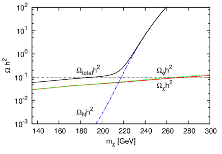
Figure 6: The $m_{\chi}$ dependence of the relic density $\Omega_{\chi}h^{2}$ (red solid line), $\Omega_{\phi}h^{2}$ (green dashed line), $\Omega_{N}h^{2}$ (blue dot-dashed line) and $\Omega_{\rm total}h^{2}$ (black solid line). The fixed parameters are shown in Table 2.

Figure 7: Contour plot for the total relic density $\Omega_{\rm total}h^{2}\sim 0.12$. The gray region is excluded by the constraint of vacuum stability. The threshold value of $m_{\chi}$ depends in particular on $M_{1}$. For the parameters given in Table 2, except for $M_{1}=500$ GeV, we find $m_{\chi}\sim 380$ GeV, for instance.

III.1 Direct detection

The current upper bound for the DM-nucleon cross section is estimated assuming the one-component DM scenario and current upper bound and future sensitivity are given in Refs. Aprile:2012nq ; Aprile:2012zx ; Akerib:2013tjd . Because the collision rate is roughly proportional to $\sigma n_{{}_{\mathrm{DM}}}$, the upper bound for the event rate can be translated to the constraint on the detection rate in the multicomponent DM scenario. The effective cross section of the nucleon corresponding to the cross section of the nucleon in the one-component DM scenario is given by

$$\sigma^{\mathrm{eff}}_{i}=\sigma_{i}\left(\frac{\Omega_{i}h^{2}}{\Omega_{\mathrm{total}}h^{2}}\right)~{}.$$ (45)

In our model, only $\phi_{R}$ and $\chi$ DM scatter with the nucleus, and the right-handed neutrino DM $N$ does not interact with nucleus at tree level. So we can neglect the $N$ contribution at the lowest order in perturbation theory. The cross sections of $\phi_{R}$ and $\chi$ are given by Barbieri:2006dq

$$\sigma_{\phi_{R}} = \frac{1}{\pi}\left(\frac{(\gamma_{5}/2)\hat{f}m_{N}}{m_{\phi_{R}}m_{h}}\right)^{2}\left(\frac{m_{N}m_{\phi_{R}}}{m_{N}+m_{\phi_{R}}}\right)^{2}~{},$$ (46)

$$\sigma_{\chi} = \frac{1}{\pi}\left(\frac{\gamma_{2}\hat{f}m_{N}}{m_{\chi}m_{h}}\right)^{2}\left(\frac{m_{N}m_{\chi}}{m_{N}+m_{\chi}}\right)^{2}~{},$$ (47)

where $\hat{f}\sim 0.3$ is the usual nucleonic matrix element Ellis:2000ds , and $m_{N}$ is the nucleon mass. Fig. 8 shows the relation between $m_{\chi}$ and the sum of the effective cross sections given in (45). The black line corresponds to the parameter space (the black line in Fig. 7) consistent with the cosmological observation of the DM relic abundance. Although as we see from Fig. 7, the scalar coupling $\gamma$ has to become large at $m_{\chi}\sim 220~{}\mathrm{GeV}$, such that the cross sections off the nucleon, $\sigma_{\chi}$ and $\sigma_{\phi_{R}}$, become large, $\sigma_{\phi_{R}}^{\rm eff}+\sigma_{\chi}^{\rm eff}$ does not change very much at $m_{\chi}\sim 220~{}\mathrm{GeV}$, because $\Omega_{\phi_{R}}$ and $\Omega_{\chi}$ both become small. We also show the result for $M_{1}=500$ GeV (the red line) in Fig. 8, where the other parameters are taken as the same as in the case with $M_{1}=300$ GeV.

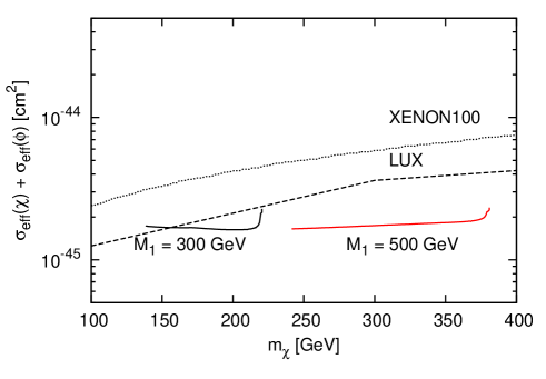
Figure 8: The relation between the $\chi$ DM mass $m_{\chi}$ and the sum of the effective cross sections given in (45). The black (red) line shows the result for $M_{1}=300$ (500) GeV. The black dotted and dashed lines show the upper limit of the spin independent cross section off the nucleon given by XENON100 Aprile:2012nq and LUX Akerib:2013tjd , respectively.

III.2 Indirect detection

For indirect detections of DM the SM particles produced by the annihilation of DM are searched. Because the semi-annihilation produces a SM particle, this process can serve for an indirect detection. In our model, especially, the SM particle from the semi-annihilation process as shown in Fig. 4 is neutrino which has a monochromatic energy spectrum Aoki:2012ub . Therefore, we consider below the neutrino flux from the Sun Silk:1985ax ; Krauss:1985aaa ; Freese:1985qw ; Gaisser:1986ha ; Griest:1986yu ; Ritz:1987mh ; Kamionkowski:1991nj ; Kamionkowski:1994dp as a possibility to detect the semi-annihilation process of DMs.

The DM particles are captured in the Sun losing their kinematic energy through scattering with the nucleus. Then captured DM particles annihilate each other. The time dependence of the number of DM $n_{i}$ in the Sun is given by

$$\dot{n}_{i} = C_{i}-C_{A}(ii\rightarrow\mathrm{SM})n_{i}^{2}-\sum_{m_{i}>m_{j}}C_{A}(ii\rightarrow jj)n_{i}^{2}-C_{A}(ij\rightarrow k\nu)n_{i}n_{j}~{},$$ (48)

where $C_{i}$ is the capture rate in the Sun, and $C_{A}$’s are the annihilation rates in the SunKamionkowski:1991nj ; Kamionkowski:1994dp ; Griest:1986yu :

$$C_{\chi} \sim 1.4\times 10^{20}f(m_{\chi})\left(\frac{\hat{f}}{0.3}\right)^{2}\left(\frac{\gamma_{2}}{0.1}\right)^{2}\left(\frac{200~{}\mathrm{GeV}}{m_{\chi}}\right)^{2}\left(\frac{\Omega_{\chi}h^{2}}{\Omega_{\mathrm{total}}}\right)^{2}~{},$$ (49)

$$C_{\phi_{R}} \sim 1.4\times 10^{20}f(m_{\phi_{R}})\left(\frac{\hat{f}}{0.3}\right)^{2}\left(\frac{\gamma_{5}}{0.2}\right)^{2}\left(\frac{200~{}\mathrm{GeV}}{m_{\phi_{R}}}\right)^{2}\left(\frac{\Omega_{\phi_{R}}h^{2}}{\Omega_{\mathrm{total}}}\right)^{2}~{},$$ (50)

$$C_{N} = 0~{},$$ (51)

$$C_{A}(ij\rightarrow\bullet) = \frac{\langle\sigma(ij\rightarrow\bullet)|v|\rangle}{V_{ij}}~{},~{}~{}~{}V_{ij}=5.7\times 10^{27}\left(\frac{100~{}\mathrm{GeV}}{\mu_{ij}}\right)^{3/2}\mathrm{cm}^{3}~{}.$$ (52)

Here $f(m_{i})$ depends on the form factor of the nucleus, elemental abundance, kinematic suppression of the capture rate, etc., varying ${\mathcal{O}}(0.01-1)$ depending on the DM mass Kamionkowski:1991nj ; Kamionkowski:1994dp . $V_{ij}$ is an effective volume of the Sun with $\mu_{ij}=2m_{i}m_{j}/(m_{i}+m_{j})$ in the nonrelativistic limit. We neglect the DM production processes in Eq.(48) like $jj\rightarrow ii$ and $jk\rightarrow iX$ because the kinetic energy of the produced particle $i$ is much larger than that corresponding to the escape velocity from the Sun, i.e. $\sim 10^{3}$ km/s Griest:1986yu ; Agrawal:2008xz . Consequently, the number of the right-hand neutrino DM cannot increase, and hence $\phi\chi\rightarrow N\nu$ is the only neutrino production process, where its reaction rate is given by $\Gamma(\nu)=C_{A}(\phi\chi\rightarrow N\nu)n_{\phi}n_{\chi}$ .

The monochromatic neutrino flux on the Earth is roughly given by $\Gamma_{\mathrm{i}nc}=\Gamma/4\pi R_{\odot}^{2}$, where $R_{\odot}$ stands for the distance to the Sun. Fig. 9 shows the $m_{\chi}$ dependence of the neutrino flux for the same parameter space (black line) as in Fig. 6. As we can see from Fig. 4 a resonance effect for the s-channel annihilation process can be achieved if $m_{\eta^{0}_{R}}\simeq m_{\phi_{R}}+m_{\chi}$. Obviously, the smaller the mass difference $m_{\eta^{0}_{R}}-(m_{\phi_{R}}+m_{\chi})$ is, the larger is the semi-annihilation cross section and hence the neutrino flux. In Fig. 9 four different values are used: $\left(m_{\eta^{0}_{R}}-(m_{\phi_{R}}+m_{\chi})~{},~{}M_{1}\right)=$ (10 GeV, 300 GeV) (black curve), (1 GeV, 300 GeV) (magenta curve), (10 GeV, 500 GeV) (red curve), and (1 GeV, 500 GeV) (blue curve), respectively. In the case that $\Omega_{N}$ dominates (so that $\Omega_{\phi}$ and $\Omega_{\chi}$ are small) the capture rates of the $\phi$ and $\chi$ DMs become small (see (48)). This is why the neutrino flux decreases after a certain value of $m_{\chi}$.

The upper limits on the defused neutrino flux from the Sun are given by the IceCube experiment Aartsen:2012kia . The upper limit on the neutrino flux produced by the annihilation of the DMs of $250$ GeV into $W^{+}W^{-}$, for instance, is $9.72\times 10^{10}$ $\mathrm{km}^{-2}\mathrm{y}^{-1}$ Aartsen:2012kia . We can see from Fig. 9 that, unfortunately, this limit is at least $10^{3}$ times larger than the monochromatic neutrino flux produced by the semi-annihilation of the $\phi$ and $\chi$ DMs. Note however, that the energy spectrum of the neutrino flux produced by the $W$ decay is different from the monochromatic neutrino. With an increasing resolution of energy and angle the chance for the observation of the semi-annihilation and hence of a multicomponent nature of DM can increase.

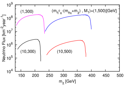
Figure 9: The neutrino flux from the Sun on the Earth against the $\chi$ DM mass. The flux is calculated from the reaction rate $\Gamma(\nu)=C_{A}(\phi\chi\rightarrow N\nu)n_{\phi}n_{\chi}$, where the numbers $n_{\phi}$ and $n_{\chi}$ are obtained by solving the evolution equation (48) numerically. We have used four different values of $m_{\eta^{0}_{R}}-(m_{\phi_{R}}+m_{\chi})$ and $M_{1}$ : $\left(m_{\eta^{0}_{R}}-(m_{\phi_{R}}+m_{\chi}),~{}M_{1}\right)$= (10 GeV, 300 GeV) (black curve), (1 GeV, 300 GeV) (magenta curve), (10 GeV, 500 GeV) (red curve), and (1 GeV, 500 GeV) (blue curve), respectively.

IV conclusion

In this paper our interest has been directed at an indirect observation of multicomponent DM systems through semi-annihilation processes of DMs, because these processes are characteristic of multicomponent DM systems. In one-component DM systems of a real scalar boson or of a Majorana fermion the monochromatic neutrino production by DM annihilation is due to the chirality of the left-handed neutrino strongly suppressed. The suppression due to the chirality is absent when DM is a complex scalar boson or a Dirac fermion. In a multicomponent DM system, too, the neutrino production is unsuppressed if it is an allowed process.

In this paper, instead of performing a model independent investigation on multicomponent DM systems we have first motivated the existence of a multicomponent DM system by extending the one-loop radiative seesaw model of Ma Ma:2006km to remove its shortcomings. In the model of Ma Ma:2006km , the lepton-number violating mass term of the inert scalar doublet has to be very small to obtain small neutrino masses. This mass term originates from a lepton-number violating quartic scalar coupling, the ”$\lambda_{5}$ coupling”, which is $\mathcal{O}(10^{-5})$ to obtain small neutrino masses for $Y^{\nu}\sim 0.01$. We therefore have considered an extension of the model such that this lepton-number violating mass, too, is radiatively generated. Consequently, the seesaw mechanism occurs at the two-loop level in the extended model Aoki:2013gzs . For this mechanism to work, we have introduced a larger unbroken discrete symmetry, $Z_{2}\times Z_{2}$, which implies that the model yields a multicomponent DM system. We emphasize that the multicomponent DM system is a consequence of the unbroken $Z_{2}\times Z_{2}$, which forbids the Dirac neutrino mass.

The DM annihilation processes can be classified to three types; standard annihilation, DM conversion and semi-annihilation. We have assumed that the right-handed neutrino $N$ and two real bosons, $\chi$ and $\phi$, are DM particles, and solved numerically the set of coupled Boltzmann equations. It has turned out that the semi-annihilation effect for the heaviest dark matter is considerably enhanced by the Boltzmann factor.

We have computed the spin-independent cross section of the dark matter particles $\phi$ and $\chi$ off the nucleon. (At the tree level there is no interaction of $N$ with the quarks.) The quantity, which should be compared with the experimental limits, is $\sigma_{\mathrm{eff}}=(\sigma_{\chi}\Omega_{\chi}+\sigma_{\phi}\Omega_{\phi})/\Omega_{\rm total}$. The predicted values of $\sigma_{\mathrm{eff}}$ have turned out to be slightly below the present limit given by LUX Akerib:2013tjd for $m_{\chi}\mathrel{\mathchoice{\vbox{\offinterlineskip\halign{$\m@th\displaystyle\hfil#\hfil$\cr>\crcr\sim\crcr} }}{\vbox{\offinterlineskip\halign{$\m@th\textstyle\hfil#\hfil$\cr>\crcr\sim\crcr} }}{\vbox{\offinterlineskip\halign{$\m@th\scriptstyle\hfil#\hfil$\cr>\crcr\sim\crcr} }}{\vbox{\offinterlineskip\halign{$\m@th\scriptscriptstyle\hfil#\hfil$\cr>\crcr\sim\crcr} }}}150$ GeV. Since the sensitivity of XENON1T Aprile:2012zx will be 2 orders of magnitude higher than that of XENON100, the predicted area will be covered by XENON1T. It should, however, be emphasized that the XENON1T experiment alone cannot decide how many dark matter particles are present. A clever choice of kinematical cuts at collider experiments could be used to explore a multi-component nature of DM Dienes:2014bka .

As mentioned above, the monochromatic neutrino production by the semi-annihilation processes $\chi~{}N\to\nu_{L}~{}\phi$, etc., is not suppressed. The time evolution of the number of the dark matter particles $n_{i}~{}(i=N,\phi,\chi$) in the Sun has been studied numerically to estimate their values at the present time, where we have set the capture rate for $N$ equal to zero. Then we have calculated the reaction rate $\Gamma(\nu)$ in the Sun, from which we have estimated the monochromatic neutrino flux coming from the Sun on the Earth and hence the monochromatic neutrino flux at the IceCube detector. It turns out that the flux is very small compared with the current IceCube sensitivity. However, the s-channel process of the semi-annihilation can be enhanced by a resonant effect: The enhanced signal is still 3 orders of magnetite smaller than the current IceCube sensitivity. Nevertheless, the higher the resolution of energy and angle is, the larger is the chance for the observation of the monochromatic neutrino and hence of a multicomponent nature of DM.

The work of M. A. is supported in part by the Grant-in-Aid for Scientific Research (Grant No. 25400250 and No. 26105509), J. K. is partially supported by the Grant-in-Aid for Scientific Research (C) from the Japan Society for Promotion of Science (Grant No. 22540271), and H. T is supported by Japan Society for the Promotion of Science (JSPS)　(Grant No. 13J05336).

References

(1)
P. Minkowski,
Phys. Lett. B 67 (1977) 421;
M. Gell-Mann, P. Ramond, and R. Slansky, in
Supergravity, eds. P. van Nieuwenhuizen and D. Z. Freedman
(North-Holland, 1979), p. 315; T. Yanagida,
in Proc. of the Workshop on
the Unified Theory and the Baryon Number in the Universe,
eds. O. Sawada and
A. Sugamoto, KEK Report No. 79-18 (Tsukuba, Japan, 1979),
p. 95;
R. N. Mohapatra and G. Senjanovic,
Phys. Rev. Lett. 44 (1980) 912.
(2)
L. M. Krauss, S. Nasri and M. Trodden,
Phys. Rev. D 67 (2003) 085002
[hep-ph/0210389];
M. Aoki, S. Kanemura and O. Seto,
Phys. Rev. Lett. 102 (2009) 051805
[arXiv:0807.0361 [hep-ph]].
(3)
E. Ma,
Phys. Rev. D 73 (2006) 077301
[hep-ph/0601225].
(4)
M. Aoki, J. Kubo and H. Takano,
Phys. Rev. D 87 (2013) 116001
[arXiv:1302.3936 [hep-ph]].
(5)
E. Ma and U. Sarkar,
Phys. Lett. B 653 (2007) 288
[arXiv:0705.0074 [hep-ph]].
(6)
Z. G. Berezhiani and M. Y. .Khlopov,
Sov. J. Nucl. Phys. 52 (1990) 60
[Yad. Fiz. 52 (1990) 96];
Z. G. Berezhiani and M. Y. .Khlopov,
Z. Phys. C 49 (1991) 73;
T. Hur, H. S. Lee and S. Nasri,
Phys. Rev. D 77, 015008 (2008)
[arXiv:0710.2653 [hep-ph]];
K. M. Zurek,
Phys. Rev. D79 (2009) 115002
[arXiv:0811.4429 [hep-ph]];
B. Batell,
Phys. Rev. D 83 (2011) 035006
[arXiv:1007.0045 [hep-ph]];
K. R. Dienes and B. Thomas,
Phys. Rev. D 85 (2012) 083523
[arXiv:1106.4546 [hep-ph]];
K. R. Dienes and B. Thomas,
Phys. Rev. D 85 (2012) 083524
[arXiv:1107.0721 [hep-ph]];
K. R. Dienes, S. Su and B. Thomas,
Phys. Rev. D 86 (2012) 054008
[arXiv:1204.4183 [hep-ph]];
D. Chialva, P. S. B. Dev and A. Mazumdar,
Phys. Rev. D 87 (2013) 6, 063522
[arXiv:1211.0250 [hep-ph]];
P. -H. Gu,
Phys. Dark Univ. 2 (2013) 35
[arXiv:1301.4368 [hep-ph]];
Y. Kajiyama, H. Okada and T. Toma,
Phys. Rev. D 88 (2013) 1, 015029
[arXiv:1303.7356];
S. Bhattacharya, A. Drozd, B. Grzadkowski and J. Wudka,
JHEP 1310 (2013) 158
[arXiv:1309.2986 [hep-ph]];
Y. Kajiyama, H. Okada and T. Toma,
Eur. Phys. J. C 74 (2014) 2722
[arXiv:1304.2680 [hep-ph]];
C. -Q. Geng, D. Huang and L. -H. Tsai,
Phys. Rev. D 89 (2014) 055021
[arXiv:1312.0366 [hep-ph]];
C. -Q. Geng, D. Huang and L. -H. Tsai,
arXiv:1405.7759 [hep-ph].
(7)
F. D’Eramo and J. Thaler,
JHEP 1006 (2010) 109
[arXiv:1003.5912 [hep-ph]];
G. Belanger, K. Kannike, A. Pukhov and M. Raidal,
JCAP 1204 (2012) 010
[arXiv:1202.2962 [hep-ph]];
I. P. Ivanov and V. Keus,
Phys. Rev. D 86, 016004 (2012)
[arXiv:1203.3426 [hep-ph]];
(8)
F. D’Eramo, M. McCullough and J. Thaler,
JCAP 1304 (2013) 030
[arXiv:1210.7817 [hep-ph]].
(9)
E. Ma,
Annales Fond. Broglie 31 (2006) 285
[arXiv:hep-ph/0607142];
E. Ma,
Mod. Phys. Lett. A23 (2008) 721
[arXiv:0801.2545 [hep-ph]];
H. Fukuoka, J. Kubo and D. Suematsu,
Phys. Lett. B 678 (2009) 401
[arXiv:0905.2847 [hep-ph]];
H. Fukuoka, D. Suematsu and T. Toma,
JCAP 1107 (2011) 001
[arXiv:1012.4007 [hep-ph]];
D. Suematsu and T. Toma,
Nucl. Phys. B 847 (2011) 567
[arXiv:1011.2839 [hep-ph]];
M. Aoki, J. Kubo, T. Okawa and H. Takano,
Phys. Lett. B 707 (2012) 107
[arXiv:1110.5403 [hep-ph]].
(10)
M. Aoki, M. Duerr, J. Kubo and H. Takano,
Phys. Rev. D 86 (2012) 076015
[arXiv:1207.3318 [hep-ph]].
(11)
R. Barbieri, L. J. Hall and V. S. Rychkov,
Phys. Rev. D 74 (2006) 015007
[arXiv:hep-ph/0603188].
(12)
L. Lopez Honorez, E. Nezri, J. F. Oliver and M. H. G. Tytgat,
JCAP 0702 (2007) 028
[arXiv:hep-ph/0612275];
E. M. Dolle and S. Su,
Phys. Rev. D 80 (2009) 055012
[arXiv:0906.1609 [hep-ph]];
M. Gustafsson, S. Rydbeck, L. Lopez-Honorez and E. Lundstrom,
Phys. Rev. D 86, 075019 (2012)
[arXiv:1206.6316 [hep-ph]].
(13)
G. Aad et al. [ATLAS Collaboration],
Phys. Lett. B 716 (2012) 1
[arXiv:1207.7214 [hep-ex]];
S. Chatrchyan et al. [CMS Collaboration],
Phys. Lett. B 716 (2012) 30
[arXiv:1207.7235 [hep-ex]].
(14)
M. Ackermann et al. [LAT Collaboration],
Phys. Rev. D 86 (2012) 022002
[arXiv:1205.2739 [astro-ph.HE]].
(16)
M. Gustafsson [ for the Fermi-LAT Collaboration],
arXiv:1310.2953 [astro-ph.HE];
F. D’Eramo and J. Thaler,
JHEP 1006, 109 (2010)
[arXiv:1003.5912 [hep-ph]];
G. Belanger, K. Kannike, A. Pukhov and M. Raidal,
JCAP 1204 (2012) 010
[arXiv:1202.2962 [hep-ph]];
F. D’Eramo, M. McCullough and J. Thaler,
JCAP 1304 (2013) 030
[arXiv:1210.7817 [hep-ph]];
G. Belanger, K. Kannike, A. Pukhov and M. Raidal,
JCAP 1301 (2013) 022
[arXiv:1211.1014 [hep-ph]];
P. Ko and Y. Tang,
JCAP 1405 (2014) 047
[arXiv:1402.6449 [hep-ph]];
G. Bélanger, K. Kannike, A. Pukhov and M. Raidal,
JCAP 1406 (2014) 021
[arXiv:1403.4960 [hep-ph]];
M. Aoki and T. Toma,
arXiv:1405.5870 [hep-ph].
(17)
T. Hambye,
JHEP 0901 (2009) 028
[arXiv:0811.0172 [hep-ph]];
C. Arina, T. Hambye, A. Ibarra and C. Weniger,
JCAP 1003 (2010) 024
[arXiv:0912.4496 [hep-ph]];
V. V. Khoze, C. McCabe and G. Ro,
arXiv:1403.4953 [hep-ph];
C. Boehm, M. J. Dolan and C. McCabe,
Phys. Rev. D 90 (2014) 023531
[arXiv:1404.4977 [hep-ph]].
(18)
G. ’t Hooft,
NATO Adv. Study Inst. Ser. B Phys. 59 (1980) 135.
(19)
R. Bouchand and A. Merle,
JHEP 1207 (2012) 084
[arXiv:1205.0008 [hep-ph]].
(20)
T. Toma and A. Vicente,
JHEP 1401, 160 (2014)
[arXiv:1312.2840, arXiv:1312.2840 [hep-ph]].
(21)
E. Ma and M. Raidal,
Phys. Rev. Lett. 87 (2001) 011802
[Erratum-ibid. 87 (2001) 159901]
[arXiv:hep-ph/0102255].
(22)
J. Adam et al. [MEG Collaboration],
Phys. Rev. Lett. 110 (2013) 201801
[arXiv:1303.0754 [hep-ex]].
(23)
K. Hayasaka,
arXiv:1010.3746 [hep-ex].
(24)
J. Beringer et al. [Particle Data Group Collaboration],
Phys. Rev. D 86 (2012) 010001.
(25)
M. Ciuchini, E. Franco, S. Mishima and L. Silvestrini,
JHEP 1308 (2013) 106
[arXiv:1306.4644 [hep-ph]].
(26)
K. Griest, D. Seckel,
Phys. Rev. D43 (1991) 3191-3203.
(27)
J. Kubo, E. Ma and D. Suematsu,
Phys. Lett. B 642 (2006) 18
[hep-ph/0604114].
(28)
G. Hinshaw et al. [WMAP Collaboration],
Astrophys. J. Suppl. 208, 19 (2013)
[arXiv:1212.5226 [astro-ph.CO]].
(29)
P. A. R. Ade et al. [Planck Collaboration],
Astron. Astrophys. (2014)
[arXiv:1303.5076 [astro-ph.CO]].
(30)
E. Aprile et al. [XENON100 Collaboration],
Phys. Rev. Lett. 109 (2012) 181301
[arXiv:1207.5988 [astro-ph.CO]].
(31)
E. Aprile [XENON1T Collaboration],
arXiv:1206.6288 [astro-ph.IM].
(32)
D. S. Akerib et al. [LUX Collaboration],
Phys. Rev. Lett. 112, 091303 (2014)
[arXiv:1310.8214 [astro-ph.CO]].
(33)
J. R. Ellis, A. Ferstl and K. A. Olive,
Phys. Lett. B 481 (2000) 304
[arXiv:hep-ph/0001005].
(34)
J. Silk, K. A. Olive and M. Srednicki,
Phys. Rev. Lett. 55 (1985) 257.
(35)
L. M. Krauss, M. Srednicki and F. Wilczek,
Phys. Rev. D 33 (1986) 2079.
(36)
K. Freese,
Phys. Lett. B 167 (1986) 295.
(37)
T. K. Gaisser, G. Steigman and S. Tilav,
Phys. Rev. D 34 (1986) 2206.
(38)
K. Griest and D. Seckel,
Nucl. Phys. B 283 (1987) 681
[Erratum-ibid. B 296 (1988) 1034].
(39)
S. Ritz and D. Seckel,
Nucl. Phys. B 304 (1988) 877.
(40)
M. Kamionkowski,
Phys. Rev. D 44 (1991) 3021.
(41)
M. Kamionkowski, K. Griest, G. Jungman and B. Sadoulet,
Phys. Rev. Lett. 74 (1995) 5174
[arXiv:hep-ph/9412213].
(42)
P. Agrawal, E. M. Dolle and C. A. Krenke,
Phys. Rev. D 79 (2009) 015015
[arXiv:0811.1798 [hep-ph]];
S. Andreas, M. H. G. Tytgat and Q. Swillens,
JCAP 0904 (2009) 004
[arXiv:0901.1750 [hep-ph]].
(43)
R. Abbasi et al. [IceCube Collaboration],
Phys. Rev. D 85 (2012) 042002
[arXiv:1112.1840 [astro-ph.HE]];
T. Tanaka et al. [Super-Kamiokande Collaboration],
Astrophys. J. 742 (2011) 78
[arXiv:1108.3384 [astro-ph.HE]].
(44)
M. G. Aartsen et al. [IceCube Collaboration],
Phys. Rev. Lett. 110 (2013) 131302
[arXiv:1212.4097 [astro-ph.HE]].
(45)
K. R. Dienes, S. Su and B. Thomas,
arXiv:1407.2606 [hep-ph].