Scaling in the Timing of Extreme Events

Abstract

Extreme events can come either from point processes, when the size or energy of the events is above a certain threshold, or from time series, when the intensity of a signal surpasses a threshold value. We are particularly concerned by the time between these extreme events, called respectively waiting time and quiet time. If the thresholds are high enough it is possible to justify the existence of scaling laws for the probability distribution of the times as a function of the threshold value, although the scaling functions are different in each case. For point processes, in addition to the trivial Poisson process, one can obtain double-power-law distributions with no finite mean value. This is justified in the context of renormalization-group transformations, where such distributions arise as limiting distributions after iterations of the transformation. Clear connections with the generalized central limit theorem are established from here. The non-existence of finite moments leads to a semi-parametric scaling law in terms of the sample mean waiting time, in which the (usually unkown) scale parameter is eliminated but not the exponents. In the case of time series, scaling can arise by considering random-walk-like signals with absorbing boundaries, resulting in distributions with a power-law “bulk” and a faster decay for long times. For large thresholds the moments of the quiet-time distribution show a power-law dependence with the scale parameter, and isolation of the latter and of the exponents leads to a non-parametric scaling law in terms only of the moments of the distribution. Conclusions about the projections of changes in the occurrence of natural hazards lead to the necessity of distinguishing the behavior of the mean of the distribution with the behavior of the extreme events.

I Introduction

The theory of self-organized criticality (SOC), introduced by Bak and collaborators, provides an appealing explanation for the distribution of sizes (and presumably durations) of many naturally occurring catastrophic events Bak_book ; Pruessner_book . Earthquakes, landslides, volcanic eruptions, rainfall, hurricanes, etc. Bak_book ; Malamud_hazards ; Peters_Deluca ; Corral_hurricanes , have been found to display power-law distributions of event sizes, which implies the absence of characteristic scales for those sizes. This means that if you ask, for instance: “how big are earthquakes in Japan?”, this innocent question has no possible answer Christensen_Moloney ; Corral_Lacidogna . In mathematical terms, this implies that after performing a scale transformation of a function describing the size of the events, the function has to remain unchanged, and the only univariate function with this property (for any dilatation or contraction) is the power law.

SOC explains this power-law behavior as coming from a self-organization process that leads the system to the critical point of a phase transition, where scale invariance is ensured. Other approaches, purely probabilistic, support the power-law tail in some cases, as described by the generalized Pareto distribution Coles . Nevertheless, the exponent of the power law in self-organized-critical systems takes such values that it is associated to an infinite expected value for the size of the events, which is unphysical; therefore, in practice, one cannot ignore finite-size effects.

When one is worried not about the size but about the time between events, the situation is a bit more involving. In fact, the waiting time is defined as the time between consecutive events when these events are above a certain threshold in size. In the usual case this approach takes place in a slow time scale, in which events happen instantaneously (in comparison with the waiting times, earthquakes are a good example). When the threshold is high enough, the events can be considered as extreme events, but there is no formal difference between these and ordinary events. Models of self-organized criticality are not very useful at this point, because, although the most common SOC models lead to a Poissonian occurrence of events and therefore to an exponential distribution of waiting times (in contrast to some observational data Boffetta ), other SOC models yield correlated avalanches Sanchez_prl ; Davidsen_pre02 One concludes from here that SOC is not about the temporal occurrence of events (in the slow time scale) but about their size (or duration).

But it is interesting anyhow to stretch the notion of scale invariance to the waiting-time problem. One deals now with two variables (size and waiting time), and in this case the scale transformation $\mathcal{T}$ is written as

$$\mathcal{T}[f(x,y)]=cf(x/a,y/b),$$ (1)

with $f(x,y)$ a bivariate function, and $a,b,c>0$, the scale factors of the transformation. When $a,b,c$ are greater than one the transformation dilates the function in its three directions; for instance, taking $a=b=c=100$ takes a function in the scale of, let us say, meters to the scale of centimeters.

The condition of scale invariance comes in this case from imposing

$$\mathcal{T}[f(x,y)]=cf(x/a,y/b)=f(x,y),$$ (2)

for all $a$. So, we are looking for a fixed point for $\mathcal{T}$ and the only solution Christensen_Moloney can be written in the form

$$f^{*}(x,y)=\frac{1}{x^{\alpha}}H\left(\frac{x}{y^{\beta}}\right)$$ (3)

with $H$ an arbitrary univariate function called scaling function and $b$ and $c$ not free but given by $c=1/{a^{\alpha}}$ and $b=a^{1/\beta}$. We will refer to this functional form of $f(x,y)$ as a scaling law. Note that for the univariate problem, described just by $x$, the scaling function has to be a constant, and then a power law is left. In fact, a power law is a particular case of a scaling law, but not the opposite, and so it is useful to keep the distinction between both concepts if one is involved with multivariate functions. The scaling law can be expressed in other, alternative, equivalent forms, as for instance,

$$f^{*}(x,y)=\frac{1}{x^{\alpha}}H_{2}\left(\frac{y}{x^{1/\beta}}\right)=\frac{1}{y^{\alpha\beta}}H_{3}\left(\frac{y}{x^{1/\beta}}\right),$$ (4)

etc., just remember that the scaling function $H$ is arbitrary.

However, one can immediately realize that, when events above a low threshold in size are compared to events with higher size, the analysis of the waiting-time does not only involve a scale transformation. Indeed, an additional coarse-graining transformation is opperating. This comes from the fact that events below the threshold need to be eliminated, in order to measure the time between consecutive events above the threshold. So, the transformation of the data comprises a coarse-graining followed by a scale transformation Corral_prl.2005 ; Corral_jstat . This is the essence of a renormalization-group transformation Christensen_Moloney .

On the other hand, one can analyze SOC models and SOC-like systems in a complementary way, not in the slow time scale in which almost instantaneous events happen but in the fast time scale inside of the events. Then, one takes a threshold not in size but in intensity (size per unit time) and measures the analogous of the waiting time, the time the signal is below threshold, which in this context is called quiet time. This approach was pursued in Ref. Paczuski_btw , where a totally different behavior was found, with a power-law distribution of quiet times (in agreement then with some observational results Boffetta ). Naturally, this framework is valid not only for SOC-like systems but for any time series from which events are defined by a process of thresholding.

This paper has as a goal to approach both kind of problems, waiting times defined in a slow time scale and quiet times defined in a fast time scale, from the point of view of scaling theory. In the next section the renormalization-group approach to the waiting-time sequence will be revisited and the precise form of the resulting scaling law will be presented for two broad class of processes, in analogy with the central limit theorem. A different scaling form for the quiet-time distribution will be used in the third section, generalizing the result for the diffusion of a Brownian particle. This yields however important consequences for the projection of extreme-event recurrence. The result is extended to the interesting case in which the right tail of the distribution is a power law, with such an exponent that the expected value of the variable is infinite. The paper illustrates in which way one has to extrapolate the statistics of ordinary events in order to infer the recurrence of extreme events in a system that shows scaling.

II Scaling in marked point processes

A point process, for our purposes, is a set of point events, i.e., instantaneous events, that occur in time Cox_Isham ; Daley_Vere_Jones ; Lowen . The simplest point process is the Poisson process, in which the events take place at a constant rate, independently of any other event. A marked point process is a point process in which the points, i.e., the events, carry some “mark”, which in our case corresponds to their size or dissipated energy.

As mentioned in the introduction, when one considers events of a large enough size, the original point process transforms or renormalizes to a new point process. Events below the threshold in size are eliminated whereas events above the threshold survive. This coarse graining or decimation is called thinning Cox_Isham or rarefaction Gnedenko in the theory of point processes. As a special class of marked point processes we will consider in this section what is called marked renewal processes Daley_Vere_Jones , in which the size of events will be independent on other sizes and on the time of occurrence of the events, and additionally, the waiting times will be independent on previous waiting times (and constitute then what is called a renewal processes Cox_Isham ; Daley_Vere_Jones , in which only the time of occurrence of the last event determines the time of the next one).

By construction, sizes are independent random variables, thus, the elimination of events below the threshold in size is equivalent to a random thinning. In this case, the waiting-time density transforms after thinning to

$$\tilde{f}_{s}(\omega)=\frac{p\tilde{f}(\omega)}{1-(1-p)\tilde{f}(\omega)}$$ (5)

where $p$ is the probability of surviving to the thinning, i.e., the probability of being above the threshold $s$, $\tilde{f}(\omega)$ is the Laplace transform of the original waiting-time probability density $f(t)$, and $\tilde{f}_{s}(\omega)$ is the Laplace transform of the waiting-time density for events of size larger than $s$, see Refs. Cox_Isham ; Gnedenko ; Corral_prl.2005 ; Corral_jstat . The Laplace transform arises because the waiting-time density for events above the threshold is the convolution of a random number of densities for all events. Then, going to Laplace space simplifies considerably the equations, as convolutions transform into simple products there.

The subsequent step of the renormalization transformation is a scale transformation. This can be done in two different ways, a trivial one and a non-trivial one, as we will show in the next two subsections.

II.1 Linear rescaling and trivial Poissonian fixed point

Let us considering the following scale transformation for the waiting-time density for events above size $s$, $f_{s}(t)\rightarrow p^{-1}f_{s}(t/p)$, or, in Laplace space,

$$\tilde{f}_{s}(\omega)\rightarrow\tilde{f}_{s}(p\omega).$$ (6)

This is because we expect that thinning increases the time scale in a $1/p$ factor, and so, in order to compensate for this fact, we perform a contraction of the function in the $x-$axis with a scale factor $a=p<1$, whereas we perform a dilatation of the function in the $y-$axis with a scale factor $c=1/p>1$, in order to keep normalization. We will see in the next subsection that this makes sense only if the mean waiting time $\langle t\rangle$ is finite. The combined effect of the thinning (5) and scale transformation yields the complete renormalization transformation $\mathcal{R}$, which is then

$$\mathcal{R}[\tilde{f}(\omega)]=\frac{p\tilde{f}(p\omega)}{1-q\tilde{f}(p\omega)}$$ (7)

with $q=1-p$. The solution of the fixed-point condition $\mathcal{R}[\tilde{f}^{*}(\omega)]=\tilde{f}^{*}(\omega)$, for all $p$, leads to the fixed-point solution or renormalization-invariant Laplace transform of the density $\tilde{f}^{*}(\omega)$. Defining a new variable $u=p\omega$ and separating the variables $\omega$ and $u$ leads to the Laplace transform of an exponential distribution, i.e.,

$$\tilde{f}^{*}(\omega)=\frac{1}{1+\ell\omega}\Rightarrow f^{*}(t)=\frac{1}{\ell}e^{-t/\ell},$$ (8)

with $\ell$ an arbitrary constant, see Refs. Cox_Isham ; Corral_prl.2005 ; Corral_jstat . This exponential distribution corresponds, due to the independence of the events in the process, to the Poisson process. In words, the Poisson process is invariant under the renormalization transformation given by Eq. (7). This is obvious if one intuitively knows the properties of the Poisson process. But it is not only that the Poisson process is invariant under the transformation (7), the results also tells us that the Poisson process is the only marked renewal process invariant under such transformation Cox_Isham ; Corral_jstat . And, even more, it is easy to show that it is also an attractor for any marked renewal process with waiting-time density with a finite mean (and whose Laplace transform exists), see Ref. Corral_jstat .

This leads us to the first scaling form or data collapse considered in this paper. Remember that in order to compare the thinned or coarse-grained distribution with the original one we perform a scale transformation of the form $f_{s}(t)\rightarrow p^{-1}f_{s}(t/p)$. This means that the fixed-point solution, i.e., the resulting probability density for very high thresholds in size fulfills the following scaling law

$$f_{s}(t)=pF(pt),$$ (9)

where the scaling function $F$ is a decreasing exponential, but we will see that $F$ can take more general forms in other cases. Therefore, if plotting $f_{s}(t)/p$ versus $pt$ yields a data collapse, i.e., a single curve, independently on the value of $p$, this implies that the scaling law is fulfilled.

Other equivalent forms of the scaling law can be obtained from the fact that the parameter $p$ gives the probability that an event has energy $E$ larger than the threshold $s$ (given that has energy larger than a reference level 0), i.e.,

$$p={\mbox{Prob}[E>s|E>0]}\simeq\frac{N_{s}}{N_{0}}$$ (10)

where $N_{s}$ is the number of events with energy above $s$. Thus, the scaling $t\rightarrow pt$ is equivalent to $N_{0}t\rightarrow N_{s}t$ but this is only valid if the window width $T$ is fixed. If time windows of different width are compared one needs to correct for this fact; so, the rescaling is equivalent to

$$R_{0}t=\frac{N_{0}}{T_{0}}t\rightarrow R_{s}t=\frac{N_{s}}{T_{s}}t$$ (11)

where $R_{s}$ is the rate of events above $s$, i.e., the number of events above $s$ per unit time. The situation of comparing different time windows is common when dealing with real data of natural catastrophes, as different sizes have different windows of completeness (see caption of Fig. 23 in Ref. Kanamori_rpp ). Then, the scaling law (9) can be alternatively written as

$$f_{s}(t)=R_{s}F(R_{s}t)=\frac{1}{\langle t\rangle}F\left(\frac{t}{\langle t\rangle}\right),$$ (12)

where we have introduced the mean waiting time $\langle t\rangle=1/R_{s}$ (which of course depends on the threshold $s$ although this is not reflected in the notation). Note that the scaling function $F$ appearing here is not exactly the same as the one in Eq. (9), as two multiplicative constants are reabsorbed in $F$. In this case the scaling law can be fulfilled by plotting the dimensionless waiting-time density $f_{s}(t)/R_{s}=\langle t\rangle f_{s}(t)$ versus the dimensionless time $R_{s}t=t/\langle t\rangle$ (in other words, plotting the waiting-time density in units of $R_{s}$ versus the waiting time in units of $\langle t\rangle$).

In order to end with the different scaling forms, if there is scale invariance in the sizes (as it happens in SOC systems, in earthquakes, etc.), then $p\propto 1/s^{\phi}$, so, an additional form for the scaling law is

$$f_{s}(t)=\frac{1}{s^{\phi}}F\left(\frac{t}{s^{\phi}}\right),$$ (13)

where again, some multiplicative constant has been dropped deliberately. This form of the scaling law is the “most natural one” in the sense that it is written in terms of the two variables of the problem, $t$ and $s$. The equivalence with the scale-invariant form of Eq. (3) is achieved by realizing that $\alpha=1/\beta=\phi$.

These scaling laws, Eqs. (9), (12), and (13), are very useful in practice, as they have been shown to show up in several natural hazards, as for instance, earthquakes Corral_prl.2004 . However, the scaling function $F$ is not provided by an exponential function alone; rather, it contains a decreasing power-law for small to intermediate times, with exponent $\nu<1$. Other authors, using a simplified model of seismicity, have argued for a different behavior, with no scaling law Saichev_Sornette_times . In any case, the simple approach in this section, based in a process with independent times and sizes, is clearly not valid for earthquakes and other natural hazards, in which important dependences exist Corral_tectono .

Other examples of a general scaling law under thinning with non-exponential scaling function include fractures Davidsen_fracture ; Baro_Corral , forest fires Corral_fires , and, curiously, printing requests Harder_Paczuski . In the case of fires only Eqs. (9) and (12) are valid, and not Eq. (13), as the fire size is not power-law distributed, for the particular data analyzed in Ref. Corral_fires . The scaling is also found in a different approach for earthquakes Bak.2002 ; Corral_pre.2003 ; Corral_physA.2004 , but there not only simple thinning is performed and the scaling under thinning should arise from the underlying scaling explained in Ref. Corral_prl.2004 . Other references provide only very indirect evidence of the scaling, as in nanofractures Astrom and in tsunamis Geist_Parsons , the problem being that no different thresholds in size are considered, although the resulting scaling functions seem to be the same as for earthquakes. The recurrence of words in texts, despite yielding a function very similar to the earthquake case, has nothing to do with thinning or renormalization Corral_words . Finally, approaches in which the threshold is imposed not in size but in intensity will be considered in the next section Bunde ; Baiesi_flares ; Laurson_upon , whereas the approach of Ref. Yamasaki is for a transformation of the original signal.

II.2 Nonlinear rescaling and non-trivial Poissonian fixed point

We explain in this subsection how the linear scaling with $p$ in Eq. (6) is not the only reasonable possibility. Let us consider instead a constant $r>1$ and perform the rescaling as $f_{s}(t)\rightarrow p^{-r}f_{s}(t/p^{r})$; this yields the (completed) renormalization transformation $\mathcal{R}$, using Eq. (5),

$$\mathcal{R}[\tilde{f}(\omega)]=\frac{p\tilde{f}(p^{r}\omega)}{1-q\tilde{f}(p^{r}\omega)}.$$ (14)

The fixed point condition leads in this case, in the same way as in the previous subsection, to

$$\tilde{f}^{*}(\omega)=\frac{1}{1+\ell\omega^{1/r}}.$$ (15)

It is easy to show Corral_jstat that, for $r>1$, this corresponds to a waiting time density with a double power-law behavior, i.e.,

$$f^{*}(t)\propto\left\{\begin{array}[]{lll}1/t^{1-1/r}&\mbox{for}&t\ll\ell^{1/r}\\ 1/t^{1+1/r}&\mbox{for}&t\gg\ell^{1/r},\\ \end{array}\right.$$ (16)

which leads to an infinite mean, as the tail is a power law with an exponent $1+1/r<2$. In the same way as for the trivial $r=1$ case, this distribution is not only the only fixed point, for a fixed $r$, but it is also an attractor for distributions with power-law tail, of the form $f(t)\sim B/t^{1+1/r}$. The case $r<1$ does not lead to well-defined probability distributions.

The non-linear rescaling with $p^{r}$ is explained by the generalized central limit theorem. Indeed, as the times $t_{i}$ have a distribution with a power-law tail, with exponent smaller than 2, the classic central limit theorem does not hold and one has instead that the total time $T$ scales as

$$T=\sum_{i=1}^{N}t_{i}\propto N^{r},$$ (17)

see Ref. Bouchaud_Georges or the Appendix I here. Thus, after thinning by a factor $p$, the time window which restores the number of events $N$ is the one that contains $N/p$ events, and this is the time window of duration $T/p^{r}$. In other words, we need to rescale time as $t\rightarrow t/p^{r}$. This is the origin of the non-linear rescaling.

In the same way as in the previous subsection, invariance under the renormalization transformation means that the invariant density is of the form

$$f_{s}(t)=p^{r}G(p^{r}t),$$ (18)

with $G$ a scaling function given by the inverse Laplace transform of Eq. (15), which we have explained has a double power-law form.

Expressions alternative to the previous rescaling can be obtained as before, by using that

$$p^{r}\simeq\frac{N_{s}^{r}/T_{s}}{N_{0}^{r}/T_{0}}\propto\frac{1}{s^{\phi r}}$$ (19)

where $N_{s}$ is the number of events with size (energy) above $s$ and we have taken into account that, in practice, the time window can be different for events above size $s$ than for events above the reference size $0$.

Therefore, the scaling law (18) can be written as

$$f_{s}(t)=\frac{1}{\sum t_{i}/N_{s}^{r}}G\left(\frac{t}{\sum t_{i}/N_{s}^{r}}\right)=\frac{N_{s}^{r-1}}{\bar{t}_{s}}G\left(\frac{N_{s}^{r-1}t}{\bar{t}_{s}}\right),$$ (20)

where $\sum t_{i}$ refers to events above threshold $s$ and $\bar{t}_{s}$ the sample mean of the waiting time above $s$ (different from the mean of the distribution, which is infinite). Note that the generalized central limit theorem implies that $\bar{t}_{s}$ diverges with the number of data, but $\sum t_{i}/N_{s}^{r}$ does not. In the case $r=1$, then $\bar{t}_{s}\simeq\langle t\rangle$ and we recover the scaling of the previous subsection. If we put the size-dependence explicitly,

$$f_{s}(t)=\frac{1}{s^{\phi r}}G\left(\frac{t}{s^{\phi r}}\right).$$ (21)

In this one and in Eq. (20) we have deliberately ignored some multiplicative constants. Comparison with the scale-invariant solution of the scale transformation, Eq. (3), shows that $\alpha=1/\beta=\phi r$.

A marked renewal process of the sort of the one in this subsection is neither implausible nor artificial. Indeed, consider that a hidden signal triggers instantaneous events (as earthquakes) when it reaches a fixed threshold and that at that point the signal is immediately reset just below the threshold. If the sizes of the events are independent and the signal cannot reach an absorbing boundary below it (this can be achieved in practice by putting the boundary of a random walk at $-\infty$, or by taking the exponentiation of the random walk, which never reaches the absorbing boundary at zero), then this leads to a marked renewal process with waiting-time density given by the so-called Lévy-Smirnov distribution, see Eq. (27), which has a right power-law tail with exponent 3/2 Redner . Iterative application of the thinning transformation leads to a different distribution, which keeps the power-law tail with exponent $3/2$ for large times but develops a new power law in the regime of small $t$, with exponent 1/2.

II.3 Paralellism with the generalized central limit theorem

Several references have pointed out the relationship between the central limit theorem and renormalization Jona_Lasinio ; Sornette_critical_book ; Sethna_book , including the generalized case Calvo . From our perspective, we can provide a clear connection between the renormalization under random thinning explained in the previous subsections and the generalized central limit theorem. The key is to consider a point process in which events are not removed randomly but deterministically, surviving a proportion $p$, in such a way that out of $1/p$ events, the $1/p-$th survives and the rest are removed (with $1/p$ integer, for instance, if $p=1/2$ the events are removed alternatively). Then, for a process in which the waiting times are independent (i.e., a renewal process), this deterministic thinning transformation can be written as

$$f_{s}(t)=[f(t)]^{\star 1/p},$$ (22)

where $f(t)$ is the probability density of the original point process, $f_{s}(t)$ the corresponding one after thinning (associated to events above size $s$), and ${\star 1/p}$ denotes convolution $1/p$ times. In Laplace space, the combined thinning plus rescaling transformation becomes

$$\mathcal{R}[\tilde{f}(\omega)]=[\tilde{f}(p^{r}\omega)]^{1/p},$$ (23)

which is the equivalent of Eq. (14), and then, the fixed point condition for $\mathcal{R}$, taking logarithms, fulfills

$$\ln\tilde{f}^{*}(\omega)=\frac{1}{p}\ln\tilde{f}^{*}(p^{r}\omega)$$ (24)

This means that $\ln\tilde{f}^{*}(\omega)$, which is a cumulant generating function, has to fulfill the scale-invariance condition. If we impose the fixed point condition for all $p$ the solution is then a power law,

$$\ln\tilde{f}^{*}(\omega)=-A\omega^{1/r},$$ (25)

and for the Laplace transform of the density we find,

$$\tilde{f}^{*}(\omega)=e^{-A\omega^{1/r}}.$$ (26)

For the case $r=1$ we recognize the Laplace transform of a Dirac’s delta function, $f^{*}(t)=\delta(t-A)$, whereas for $r=2$ we get

$$f^{*}(t)=e^{-A^{2}/(4t)}\frac{A}{2\sqrt{\pi}\,t^{3/2}},$$ (27)

which is sometimes called Lévy-Smirnov distribution. For any $r>1$ the fixed-point distribution has a power-law tail, for large times, with exponent $1+1/r<2$ (with infinite mean therefore). As one can see in Appendix I, these distributions are also attractors, with different domains of attraction. The case $r=1$ yields the classic law of large numbers Feller , in the form of the attractiveness of the Dirac’s delta function, whereas $r>1$ leads to a certain case of the generalized central limit theorem Bouchaud_Georges .

III Scaling in the quiet times of time series

The previous section was devoted to point processes in which the size of the events was larger than some threshold. From the point of view of SOC, we were looking at the system in the slow time scale. Here we analyze the equivalent problem in the fast time scale (if there are two time scales), in order to see similarities and differences. Our approach will be also valid for non-SOC systems, with only one time scale, as usual time series. The procedure consists simply in introducing a threshold in the value of the signal (intensity or activity in the SOC language) and define the quiet time as the time the signal is below threshold. Several papers have used this approach before Bunde ; Baiesi_flares ; Laurson_upon . Nevertheless, the results will be of broader applicability.

III.1 Non-parametric scaling form

In Appendix II we consider an intensity signal modeled by a Brownian noise between two absorbing boundaries (the zero-intensity state and the threshold) and show how the quiet-time distribution fulfills a scaling law. Let us generalize here that scaling law, replacing the Brownian exponent 3/2 by a generic and undefined exponent $\nu$, and considering a generic scaling function $G$, then we write

$$f_{\tau}(t)=\frac{1}{\tau^{\nu}}G\left(\frac{t}{\tau}\right),$$ (28)

where the scale parameter is now called $\tau$, and enters as a subindex of the probability density $f_{\tau}(t)$ to indicate the dependence on the threshold (as $\tau$ depends on it). The density is defined for $t>m$ and is zero otherwise. The scaling function $G$ has to decrease, for large arguments, fast enough, which in our case means faster than $1/t^{6}$, as we are interested, at most, in the calculation of the third moment (i.e., we ask not only for the finiteness of the expected value of $t^{3}$, which is $\langle t^{3}\rangle$, but also for the finiteness of the second moment of $t^{3}$, which is $\langle t^{6}\rangle$). This is the “worst” scenario and in some case $G$ can decay slower than $1/t^{6}$, the main requirement being that the moments involved in the equations are finite, as well as their variances.

As shown in Appendix II, the scaling function $G$ can be a bit complicated and it is more convenient to write the scaling law in a slightly modified form, separating a power-law behavior for intermediate values from the rest of the scaling function,

$$f_{\tau}(t)=\frac{K}{\tau}\left(\frac{\tau}{t}\right)^{\nu}F\left(\frac{t}{\tau}\right)$$ (29)

for $t>m$, where we assume that the function $F$ tends to a positive constant at zero, and $K$ is a normalization constant. This scaling form also comprises the scaling laws of the previous section, taking $0<\nu<1$ for the case of earthquakes Corral_prl.2004 , and $\nu=0$ for the trivial Poisson fixed point of uncorrelated point processes. As, for small arguments, the scaling function $F$ tends to a constant and decreases “fast enough” for large arguments, the scale parameter $\tau$ separates at least two regimes, being the one for $t\gg\tau$ the corresponding for extreme events; in other words, $\tau$ sets the scale of extreme events. It is worth mentioning that here we use a broader definition of scaling function than the one of Ref. Christensen_EPJB , as there it is enforced that the scale parameter $\tau$ only appears in the argument of the scaling function, and not outside. The use of that prescription or the use of our scaling form is a matter of choice and has no fundamental implications.

Thus, in the case $\nu<1$ we can take $m=0$ and verify that $K$ is a constant indeed and then it is reabsorbed into the scaling function (i.e., $K=1$). However, for $\nu>1$ one finds that $K$ is not a true constant but proportional to $(m/\tau)^{\nu-1}$, and then $m$ cannot be zero. The scaling law for $\nu>1$ turns out to be

$$f_{\tau}(t)=\frac{1}{m}\left(\frac{m}{t}\right)^{\nu}F\left(\frac{t}{\tau}\right)\mbox{ for }t>m>0.$$ (30)

Both cases, $\nu<1$ and $\nu>1$, can be summarized into a unique scaling law,

$$f_{\tau}(t)=\frac{1}{\theta}\left(\frac{\theta}{t}\right)^{\nu}F\left(\frac{t}{\tau}\right)\mbox{ for }t>m,$$ (31)

with $\theta=\tau$ and $m=0$ for $\nu<1$ and with $\theta=m$ and $m>0$ for $\nu>1$. Note that for $\nu>1$ we can write

$$f_{\tau}(t)=\frac{1}{m}\left(\frac{m}{\tau}\right)^{\nu}G\left(\frac{t}{\tau}\right),$$ (32)

although for $\nu<1$ we still have $f_{\tau}(t)=G(t/\tau)/\tau$.

The scaling law becomes more apparent substituting the scale parameter $\tau$ by its scaling with the threshold $L$ (assuming it happens, as for a Brownian particle), i.e., $\tau\propto L^{\phi}$. In this way

$$f_{\tau}(t)=\frac{1}{L^{\phi}}G\left(\frac{t}{L^{\phi}}\right),$$ (33)

for $\nu<1$, and

$$f_{\tau}(t)=\frac{1}{m}\left(\frac{m}{L^{\phi}}\right)^{\nu}G\left(\frac{t}{L^{\phi}}\right),$$ (34)

for $\nu>1$.

If one is interested in describing the distribution, instead of by its probability density, by its cumulative or survivor function, defined by $S_{\tau}(t)=\int_{t}^{\infty}f_{\tau}(t^{\prime})dt^{\prime}$, one has that

$$S_{\tau}(t)\propto\left\{\begin{array}[]{ll}I(t/\tau)&\mbox{ for }\nu<1,\\ (m/\tau)^{\nu-1}I(t/\tau)&\mbox{ for }\nu>1,\\ \end{array}\right.$$ (35)

with $I$ a new scaling function. Anyhow, for us the most useful quantity will be the density, $f_{\tau}(t)$.

At this point it becomes interesting to see the consequences of the scaling law on the moments of the distribution (moments about the origin, $t=0$). One can easily calculate the mean for $\tau\gg m$ Christensen_Moloney ,

$$\langle t\rangle=\int_{m}^{\infty}tf_{\tau}(t)dt\propto\left\{\begin{array}[]{ll}\tau&\mbox{ for }\nu<1,\\ m(\tau/m)^{2-\nu}&\mbox{ for }1<\nu<2,\\ m&\mbox{ for }2<\nu,\\ \end{array}\right.$$ (36)

and in the same way the second moment,

$$\langle t^{2}\rangle=\int_{m}^{\infty}t^{2}f_{\tau}(t)dt\propto\left\{\begin{array}[]{ll}\tau^{2}&\mbox{ for }\nu<1,\\ m^{2}(\tau/m)^{3-\nu}&\mbox{ for }1<\nu<3,\\ m^{2}&\mbox{ for }3<\nu,\\ \end{array}\right.$$ (37)

The idea is that the scaling forms we have seen up to now are parametric, in the sense that depend on unknown parameters $\nu$ and $\tau$. The exponent $\nu$ may be calculated with careful methods Corral_Deluca , but the scale parameter needs a particular parameterization of the scaling function $G$, which may me arbitrary. An alternative, free of these restrictions, is to use a non-parametric scaling form.

For the case $\nu<1$ we know that $\tau\propto\langle t\rangle$ (see Eq. (36)) and then we recover the scaling form proposed in the previous section Corral_prl.2004 ,

$$f_{\tau}(t)=\frac{1}{\langle t\rangle}G\left(\frac{t}{\langle t\rangle}\right),$$ (38)

where the constant of proportionality between $\tau$ and $\langle t\rangle$ is reabsorbed in $G$. We could also have used that $\tau\propto\sqrt{\langle t^{2}\rangle}$, but the scaling with $\langle t\rangle$ is preferred as the computation of the first moment has a smaller error than that of the second moment.

For the new case $1<\nu<2$ we cannot apply the previous scaling, and instead, we have, on the one hand, dividing Eqs. (37) and (36),

$$\tau\propto\frac{\langle t^{2}\rangle}{\langle t\rangle},$$ (39)

and, on the other hand, isolating from Eq. (36) and substituting in the previous one,

$$\left(\frac{m}{\tau}\right)^{\nu}\propto\frac{\langle t\rangle}{m}\left(\frac{m}{\tau}\right)^{2}\propto m\frac{\langle t\rangle^{3}}{\langle t^{2}\rangle^{2}}.$$ (40)

Substituting this into the scaling law (32) we get

$$f_{\tau}(t)=\frac{\langle t\rangle^{3}}{\langle t^{2}\rangle^{2}}\,G\left(\frac{\langle t\rangle}{\langle t^{2}\rangle}\,t\right),$$ (41)

see Refs. Rosso ; Peters_Deluca . Figure 1 shows an example of this rescaling.

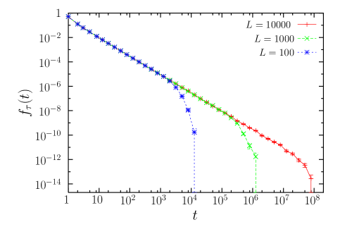
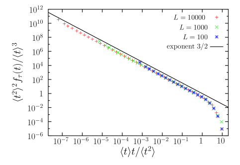
Figure 1: (a) Probability densities for the first-passage time of a random walk between two absorbing boundaries. Every time step the walker has probability 1/2 of increasing its position by 1 and the same probability to decrease it by 1. The initial position is one unit below the threshold. The time steps take place every 0.5 time units (in order that the first-passage times take values 1, 2, 3, etc.) Different values of the threshold $L$ are considered. (b) Same distributions under the non-parametric rescaling given by Eq. (41). The data collapse is an indication of the fulfillment of the scaling law.

An intermediate, semi-parametric scaling form is also possible, if one knows the exponent $\nu$ but not the scale parameter $\tau$, in this case one may write, from Eq. (36), $\tau\propto m(\langle t\rangle/m)^{1/(2-\nu)}$ and from here,

$$f_{\tau}(t)=\frac{1}{m}\left(\frac{m}{\langle t\rangle}\right)^{\nu/(2-\nu)}G\left(\left(\frac{m}{\langle t\rangle}\right)^{1/(2-\nu)}\frac{t}{m}\right),$$ (42)

see Refs. Corral_hurricanes ; Pruessner_comment .

For completeness, it is interesting to analyze the scaling behavior for $2<\nu<3$. In this case the mean does not depend on the scale parameter, and we have to replace the mean with the third moment, which scales as $\langle t^{3}\rangle\propto m^{3}(\tau/m)^{4-\nu}$, valid for $1<\nu<4$. Using also the scaling for $\langle t^{2}\rangle$ and dividing both,

$$\frac{\langle t^{3}\rangle}{\langle t^{2}\rangle}\propto\tau,$$ (43)

and isolating from the scaling of $\langle t^{2}\rangle$,

$$\left(\frac{m}{\tau}\right)^{\nu}\propto\frac{\langle t^{2}\rangle}{m^{2}}\left(\frac{m}{\tau}\right)^{3},$$ (44)

and substituting the scaling of $\tau$,

$$\left(\frac{m}{\tau}\right)^{\nu}\propto m\frac{\langle t^{2}\rangle^{4}}{\langle t^{3}\rangle^{3}},$$ (45)

and substituting in the scaling law (32),

$$f_{\tau}(t)=\frac{\langle t^{2}\rangle^{4}}{\langle t^{3}\rangle^{3}}G\left(\frac{\langle t^{2}\rangle t}{\langle t^{3}\rangle}\right).$$ (46)

valid in principle for $1<\nu<3$ but useful in practice for $2<\nu<3$. A semi-parametric scaling form, if one knows $\nu$ but not $\tau$, can be found from the fact that $m/\tau\propto(m^{2}/\langle t^{2}\rangle)^{1/(3-\nu)}$ and then,

$$f_{\tau}(t)=\frac{1}{m}\left(\frac{m^{2}}{\langle t^{2}\rangle}\right)^{\nu/(3-\nu)}G\left(\left(\frac{m^{2}}{\langle t^{2}\rangle}\right)^{1/(3-\nu)}\frac{t}{m}\right).$$ (47)

The different non-parametric scaling functions, for the different ranges of $\nu$, are summarized in Table 1.

Scaling has important consequences for the projection of extreme events. We have presented our scaling analysis for the waiting time or quiet time $t$ of events, but of course the results are more general, being suitable for other variables different than $t$. Considering the scaling form (29), valid for $\nu<1$, we have seen that $\langle t\rangle\propto\tau$; in consequence, an increase in the mean has associated a proportional increase in the scale of extreme events, quantified by $\tau$. But for the scaling form (30), linked to $\nu>1$, the mean does not scale linearly with the scale $\tau$ of extreme events. In the case $1<\nu<2$ we have $\langle t\rangle\propto\tau^{2-\nu}$ (see Eq. (36)); this means, for instance, that a two-fold increase in the mean of the distribution implies an increase of a factor $2^{1/(2-\nu)}$ in the scale of the largest, extreme events (a quadruplication if $\nu=3/2$ and much higher if $\nu$ approaches 2). This is the case of the energy released by hurricanes Corral_hurricanes , for which the mean of the distribution increases with sea-surface temperature, but the increase of the largest energies is higher. On the other hand, if $\nu>2$, the mean and the scale of extreme events become unrelated, as $\langle t\rangle\propto m$ (i.e., a constant). As a recent publication states, “much of today’s research represents climate change in terms of changes to the annual or seasonal averages”, whereas the subject of major concern is the change corresponding to the most devastating, extreme events Perez_ngeo .

Table 1: Non-parametric rescaling of the axes coming from the scaling law $f_{\tau}(t)=\theta^{-1}(\theta/t)^{\nu}F(t/\tau)$ with $\theta=\tau$ for $\nu<1$ and with $\theta=m$ for $\nu>1$. The scaling function $F$ decays fast enough in order that the moments up to $\langle t^{3}\rangle$ and their variances are not infinite. The equivalent rescaling for the survivor function $S_{\tau}(t)=(\theta/\tau)^{\nu-1}I(t/\tau)$ is also included.

	abscissa	ordinate for $f_{\tau}(t)$	ordinate for $S_{\tau}(t)$
$\nu<1$	$t/\langle t\rangle$	$\langle t\rangle f_{\tau}(t)$	$S_{\tau}(t)$
$1<\nu<2$	$\langle t\rangle t/\langle t^{2}\rangle$	$\langle t^{2}\rangle^{2}f_{\tau}(t)/\langle t\rangle^{3}$	$\langle t^{2}\rangle S_{\tau}(t)/\langle t\rangle^{2}$
$1<\nu<3$	$\langle t^{2}\rangle t/\langle t^{3}\rangle$	$\langle t^{3}\rangle^{3}f_{\tau}(t)/\langle t^{2}\rangle^{4}$	$\langle t^{3}\rangle^{2}S_{\tau}(t)/\langle t^{2}\rangle^{3}$

III.2 Case with infinite mean generalized

In the previous section (subsec. II.2) we saw how, in some peculiar cases, marked renewal processes do not converge under thinning to the Poisson process but to a process in which the waiting-time density shows a double (decreasing) power-law behavior, with an exponent between 0 and 1 for short times, and another exponent between 1 and 2 for long times (and with the sum of both exponents equal to 2). This behavior in the right tail is associated to an infinite mean-waiting time $\langle t\rangle$.

In this subsection we study the proper scaling of such distributions in a more general framework, considering distributions (no matter if for the waiting time, the quiet time, or any other variable showing scaling) as those given by Eqs. (31) and (32),

$$f_{\tau}(t)=\frac{1}{\theta}\left(\frac{\theta}{t}\right)^{\nu}F\left(\frac{t}{\tau}\right)=\frac{1}{\theta}\left(\frac{\theta}{\tau}\right)^{\nu}G\left(\frac{t}{\tau}\right),$$ (48)

defined for $t>m,$ with $m=0$ and $\theta=\tau$ if $\nu<1$ and with $m>0$ and $\theta=m$ if $\nu>1$. Note that $t$ is the variable and $\tau$ is the scale parameter. The difference with the previous subsection is that $f_{\tau}(t)$ has now a (right) power-law tail, with exponent between 1 and 2, i.e., for large arguments $G$ decays as a power law with exponent $1+\rho$, with $0<\rho<1$, and then $\langle t\rangle$ is infinite, as in subsec. II.2. But in contrast to that subsection, and in the same way as in the previous one, $F$ goes to a constant for small arguments, so $G$ goes as another (decreasing) power law there, with exponent $\nu$, with no particular relation between both exponents ($1+\rho$ and $\nu$).

In the same way as before, we are interested in relating the mean value of the variable with its scale parameter $\tau$, with the difference that now the expected value $\langle t\rangle$ is infinite and we have to emphasize the role of the sample mean, $\bar{t}=\sum_{i}t_{i}/N$ (which is always finite if $N$ is finite). The power-law tail of the distribution means that $f_{\tau}(t)$ goes, for large enough $t$ as $B/t^{1+\rho}$. We can realize that a scale parameter is given by $\tau=B^{1/\rho}$. Applying the results of the generalized central-limit theorem explained in Appendix I, we get that

$$\sum_{i=1}^{N}t_{i}\sim[-\Gamma(\rho)BN]^{1/\rho},$$ (49)

where the symbol “$\sim$” means that, for large $N$, $\sum_{i}t_{i}$ is distributed following a certain (Lévy-stable) distribution whose scale parameter is $[-\Gamma(\rho)BN]^{1/\rho}$. From here we get that the scale parameter $\tau$ of $f_{\tau}(t)$ can be related to $\sum_{i}t_{i}$ and therefore with the sample mean as

$$\tau=B^{1/\rho}\sim\frac{\sum_{i=1}^{N}t_{i}}{[-\Gamma(\rho)N]^{1/\rho}}\propto\frac{\bar{t}}{N^{1/\rho-1}}.$$ (50)

The case $\nu<1$, for which $\theta=\tau$, can be obtained straightforwardly from Eq. (48), which leads to

$$f_{\tau}(t)=\frac{N^{1/\rho-1}}{\bar{t}}G\left(\frac{N^{1/\rho-1}t}{\bar{t}}\right)$$ (51)

and is of the same form as Eq. (20). For the new case $\nu>1$ we need to consider $\theta=m$, and from Eq. (48), substituting $\tau$, we get

$$f_{\tau}(t)=\frac{1}{m}\left(\frac{mN^{1/\rho-1}}{\bar{t}}\right)^{\nu}G\left(\frac{N^{1/\rho-1}t}{\bar{t}}\right).$$ (52)

Table 2 summarizes the results for $\nu<1$ and $\nu>1$.

Table 2: Semi-parametric rescaling of the axes coming from the scaling law $f_{\tau}(t)=\theta^{-1}(\theta/t)^{\nu}F(t/\tau)$ with $\theta=\tau$ for $\nu<1$ and with $\theta=m$ for $\nu>1$. The right tail of $F$ decays slow enough in order that $\langle t\rangle$ is infinite. In contrast, the sample mean $\bar{t}$ is finite if $N$ is finite.

	abscissa	ordinate
$\nu<1$	$N^{1/\rho-1}t/\bar{t}$	$\bar{t}f_{\tau}(t)/N^{1/\rho-1}$
$\nu>1$	$N^{1/\rho-1}t/\bar{t}$	$(\bar{t})^{\nu}f_{\tau}(t)/N^{\nu(1/\rho-1)}$

Notice that, in contrast to the case of previous subsection, where the tail of the distribution was decaying fast enough, we do not arrive at non-parametric forms of the scaling laws. We can get ride of the scale parameter $\tau$ but the results still depend on the parameter $\rho$ and, if $\nu>1$, also on $\nu$. The reason is that, for fixed number of data, the (sample) moments do not depend on the exponents, and therefore the exponents cannot be isolated from the moments. Indeed, in order to calculate the second sample moment $\bar{t^{2}}$ we can use that $t^{2}$ is also power-law distributed with exponent $1+\rho/2$ (and a multiplying constant $B/2$) and we can apply in the same way the generalized central-limit theorem to get

$$\sum_{i=1}^{N}t_{i}^{2}\sim\left[-\Gamma(\rho/2)\frac{B}{2}N\right]^{2/\rho},$$ (53)

and from here

$$\tau^{2}=B^{2/\rho}\sim\frac{\bar{t^{2}}}{N^{2/\rho-1}}.$$ (54)

For higher order moments the results are analogous, and so we cannot isolate neither the exponent $\nu$ nor $\rho$ from here (for a fixed $N$).

Both forms of the scaling law, for $\nu<1$ and for $\nu>1$, can be tested from simulations. We generate double-power-law distributed values of $t$ by the rejection method, first generating a (simple) power law with exponent $1+\rho$ for $t>1$ and then rejecting the value of $t$ if it yields a $t^{\epsilon}/(k+t^{\epsilon})$ smaller than a uniform random number $u$. This leads to a double-power-law distribution, with scale parameter $\tau=k^{1/\epsilon}$ and with exponents $\nu=1+\rho-\epsilon$ and $1+\rho$ for small and large $t$, respectively (if $\epsilon>0$, if not, the situation is reversed). Figure LABEL:figdos shows an example for $\nu>1$.

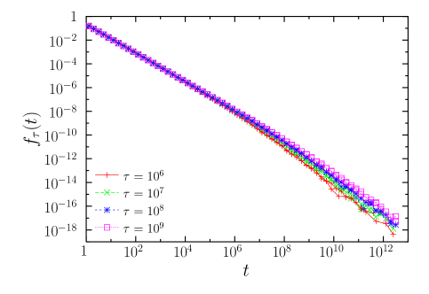
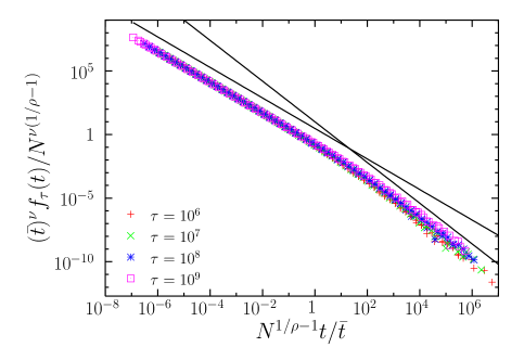
Figure 2: (a) Probability densities for simulated double-power-law distributions, with parameters $\nu=1.2$, $1+\rho=1.6$, and $m=1$, for different values of the scale parameter $\tau$. Two different values of $N$ are used for each $\tau$, these are $N=10^{5}$ and $N=10^{6}$. (b) Same distributions after a semi-parametric rescaling of the axes, following Eq. (52). The collapse of data indicates the fulfillment of the scaling law. The straight lines are power laws with exponents 1.2 and 1.6.

IV Summary

We have seen how scaling laws can arise in the waiting time or quiet time between extreme events. We consider two scenarios. The first one deals with point processes, for which events happen instantaneously in comparison with the waiting time between events. This corresponds to the slow time scale of driving in SOC systems. It is shown that scaling might arise as an attractive fixed point of a renormalization transformation, consisting of thinning of events below a threshold in size plus a rescaling of the time axis (so, it is considered that high enough thresholds lead to the fixed-point solution). For processes without correlations, the resulting scaling law contains an exponential scaling function (characteristic of a Poisson process) if the mean waiting time between the original events has a finite mean. In contrast, if the mean waiting time is infinite, a non-trivial scaling function arises, with a double-power-law behavior. Different forms of the scaling law are shown in terms of the probability $p$ of surviving the thinning process, the mean waiting time for the renormalized events, or the distribution of events above size $s$. The results are critically dependent on whether $\langle t\rangle$ is finite or infinite. As a corollary, a slight change in the renormalization procedure (removing events deterministically instead of randomly) leads to a direct derivation of the law of large numbers and the generalized central-limit theorem (for the case of maximum asymmetry) Gnedenko .

The second scenario contemplates time series, and the variable of interest is the quiet time (the time the signal is below a threshold), representing again but in a different way the time between extreme events. In the SOC framework this would correspond to look at the system in the fast time scale inside the avalanches. In this case scaling laws might show up from the first-passage time of diffusion processes that model the signal, in the limit of high enough thresholds. The scaling law yields scaling functions different than the ones from point processes, with a decaying power law for short times (except for the shortest times) and a much faster decay for long times. Using the dependence of the moments of the distribution on the scale parameter and on the power-law exponent we can replace the latter ones in terms of the former ones and obtain a non-parametric scaling law, depending only on the moments. The particular equation for the scaling law depends on the value of the power-law exponent; in particular we have distinguished $\nu<1$ (trivial scaling), $1<\nu<2$, and $1<\nu<3$. Finally, this result is generalized for the case in which the waiting-time distribution does not decay fast enough for long times but slow enough in such a way that the mean waiting time becomes infinite. No non-parametric scaling is possible then and one obtains a semi-parametric scaling in which the dependence on the scale parameter can be substituted by the dependence on the sample moments, but the exponents cannot be replaced. Additionally, important lessons for the projection of extreme events are derived from the different scaling of the mean of the distribution and the scale of extreme events.

V Acknowledgements

This paper is a re-elaboration of a talk of the author at the EXEV14 workshop; invitation by A. Deluca, H. Kantz and N. W. Watkins is gratefully acknowledged. The author is indebted to N. R. Moloney for pointing to the references relating renormalization and the central limit theorem and to G. Pruessner for his influential lectures at the Joint CRM-Imperial College School in Complex Systems. Research expenses were founded by projects FIS2009-09508, from the disappeared Spanish MICINN, FIS2012-31324 from Spanish MINECO, and 2009SGR-164, from AGAUR. This work is also associated to 2014SGR-1307.

VI Appendix I: Generalized central limit theorem from renormalization

Remember that in the (generalized-) central-limit-theorem scenario one sums independent identically distributed random variables and then the sum is rescaled in order that the resulting distribution is comparable to the original distribution of the individual variables. We showed in subsec. II.3 that this is exactly the same problem one finds for the waiting time of extreme events when these happen in a deterministic way, being the $1/p-$th out of $1/p$ events an extreme event, and the rest, $1/p-1$ events, being ordinary events, which are removed. In this way, the connection with a renormalization transformation is direct. Introducing $n=1/p$, and assuming $n$ is a natural number, we know from subsec. II.3 that the cumulant generating function of the sum and rescaling of these $n$ random variables (in our case waiting times, but we put ourselves here in a more general context) transforms as

$$\mathcal{R}[\ln\tilde{f}(\omega)]=n\ln\tilde{f}\left(\frac{\omega}{n^{r}}\right),$$ (55)

i.e., suffers a simple scale transformation under this operation, where $\ln\tilde{f}(\omega)$ is the cumulant generating function of the original random variables (which is the logarithm of the Laplace transform $\tilde{f}(\omega)$ of the probability density $f(t)$). In subsec. II.3 we saw the fixed points of this transformation (i.e., the distributions which are stable under renormalization) and now we explore the attractiveness of these fixed points, which is what provides the content for the central limit theorem.

VI.1 Existence of all moments

The simplest case corresponds to the common situation of an initial probability density whose moments exist and are finite (non-infinite). If the cumulant generating function exists, it is well know that its expansion will be

$$\ln\tilde{f}(\omega)=-\langle t\rangle\omega+\mathcal{O}(\omega),$$ (56)

where $\mathcal{O}(\omega)$ refers to terms that are of higher order than linear in $\omega$ (just expand by Taylor the exponential factor $e^{-\omega t}$ in the Laplace transform, take the logarithm of the resulting series and expand again the logarithm). Applying the renormalization transformation to the expansion of $\ln\tilde{f}(\omega)$ one gets

$$\mathcal{R}[\ln\tilde{f}(\omega)]=n\left(-\langle t\rangle\frac{\omega}{n^{r}}+\mathcal{O}(\omega/n^{r})\right),$$ (57)

and imposing linear rescaling, $r=1$, leads, after successive iterations of the transformation (or, equivalently, after taking the limit $n\rightarrow\infty$) to

$$\mathcal{R}[\cdots\mathcal{R}[\ln\tilde{f}(\omega)]\cdots]\rightarrow-\langle t\rangle\omega,$$ (58)

where note that all non-linear terms vanish (we are assuming that $\langle t\rangle>0$). We already saw that this is the logarithm of the Laplace transform of a Dirac’s delta function, and therefore

$$\mathcal{R}[\cdots\mathcal{R}[f(t)]\cdots]\rightarrow\delta(t-\langle t\rangle)$$ (59)

(we use the same notation for the renormalization transformation operating over $f(t)$, over its Laplace transform, or over the cumulant generating function). Although we are in the context of the central limit theorem, this trivially-looking result is nothing else than a weak version of the law of large numbers Feller , perhaps the most fundamental result in probability theory and statistics, ensuring that the arithmetic mean of a sample converges to the expected value of the distribution (if this expected value exists and is not infinite, and the same for the rest of the moments).

It is noteworthy that the equivalent of the law of large numbers when the number of variables that are added is not fixed but random, following a geometrical distribution, is the exponential distribution (as we saw in subsec. II.1). On the other hand, if a fixed number of variables are summed but the mean is zero one obtains the classic central-limit result in the form of a Gaussian distribution, which is of no interest here, but see Ref. Bouchaud_Georges .

VI.2 Power laws and power-law tails

The “non-trivial” case corresponds to a distribution $f(t)$ which is a power law, or at least that has a power-law upper tail. In the first case $f(t)=B/t^{1+\rho}$, for $t>m>0$, with $\rho>0$ and $B=\rho m^{\rho}$ (normalization condition). The Laplace transform of the density can be expressed in terms of the incomplete gamma function,

$$\tilde{f}(\omega)=B\int_{m}^{\infty}e^{-\omega t}t^{-\rho-1}dt=B\omega^{\rho}\Gamma(-\rho,m\omega).$$ (60)

Using the expansion of this function (see 6.5.29 of Ref. Abramowitz ),

$$\Gamma(\gamma,z)=\Gamma(\gamma)-z^{\gamma}\sum_{n=0}^{\infty}\frac{(-z)^{n}}{(\gamma+n)n!},$$ (61)

valid for $\gamma\neq 0,-1,-2,-3\dots$, we can write

$$z^{\rho}\Gamma(-\rho,z)=z^{\rho}\Gamma(-\rho)-\sum_{n=0}^{\infty}\frac{(-z)^{n}}{(n-\rho)n!}$$ (62)

$$=\frac{1}{\rho}\left[\rho\Gamma(-\rho)z^{\rho}+\left(1+\frac{\rho z}{1-\rho}+\mathcal{O}(z)\right)\right],$$ (63)

for $\rho\neq 0,1,2,\dots$ From here, taking the logarithm, and using its expansion around $z=1$,

$$\ln\left[z^{\rho}\Gamma(-\rho,z)\right]=-\ln\rho+\rho\Gamma(-\rho)z^{\rho}+\frac{\rho z}{1-\rho}+\mathcal{O}(z),$$ (64)

which we can substitute in the expression of $\ln\tilde{f}(\omega)$, from Eq. (60), so

$$\ln\tilde{f}(\omega)=\ln\frac{B}{m^{\rho}}+\ln\left[m^{\rho}\omega^{\rho}\Gamma(-\rho,m\omega)\right]$$ (65)

$$=\rho\Gamma(-\rho)m^{\rho}\omega^{\rho}+\frac{\rho m\omega}{1-\rho}+\mathcal{O}(\omega),$$ (66)

where we have used that $B=\rho m^{\rho}$. Applying the renormalization transformation we arrive at

$$\mathcal{R}[\ln\tilde{f}(\omega)]=n\ln\tilde{f}\left(\frac{\omega}{n^{r}}\right)$$ (67)

$$=n\left(\rho\Gamma(-\rho)m^{\rho}\left(\frac{\omega}{n^{r}}\right)^{\rho}+\frac{\rho m\omega/n^{r}}{1-\rho}+\mathcal{O}(\omega/n^{r})\right).$$ (68)

We can distinguish two situations here. On the one hand, if $\rho>1$ in order to have a well-defined limiting distribution we need to take $r=1$, which yields, in the same way as in the trivial case, the delta function corresponding to the law of large numbers,

$$\mathcal{R}[\dots\mathcal{R}[\ln\tilde{f}(\omega)]\dots]\rightarrow-\frac{\rho m\omega}{\rho-1},$$ (69)

so,

$$\mathcal{R}[\dots\mathcal{R}[f(t)]\dots]\rightarrow\delta\left(t-\frac{\rho m}{\rho-1}\right).$$ (70)

Notice that for the power-law distribution with $\rho>1$ the expected value is $\langle t\rangle=\frac{\rho m}{\rho-1}$, but the other moments can diverge and still the law of large numbers holds in this case.

On the other hand, a different situation corresponds to $\rho<1$, and in order to have a well-defined limit we need to take $r=1/\rho$, and then

$$\mathcal{R}[\dots\mathcal{R}[\ln\tilde{f}(\omega)]\dots]\rightarrow\rho\Gamma(-\rho)m^{\rho}\omega^{\rho},$$ (71)

which corresponds to a Laplace transform given by $\tilde{f}^{*}(\omega)=\exp(B\Gamma(-\rho)\omega^{\rho})$. This yields Lévy-stable distributions with maximal asymmetry Bouchaud_Georges . As far as the author knows, the Laplace transform only can be inverted for $\rho=1/2$, yielding the sometimes called Lévy-Smirnov distribution, Eq. (27), with $A=-B\Gamma(-1/2)=2\sqrt{\pi}B$. For general values of $\rho$ (in the range $(0,1)$) it can be shown that the limiting distribution behaves, for large $t$ as $f^{*}(t)\propto 1/t^{1+\rho}.$ So, when power-law distributed variables, with exponent $1+1/r<2$, are summed, the way to rescale them is not by the number of terms $n$ but by $n^{r}$. With this “strange” average we get convergence to a Lévy stable distribution, but not to a Dirac’s delta distribution, so, no generalized form of the law of large numbers holds. Rather, this result is considered to belong to the generalized central-limit theorem, although one is not dealing with the center of the distribution.

In the second “non-trivial” case we have a distribution which asymptotically (for large $t$) is a power law, $f(t)\sim B/t^{1+\rho}$, with $B$ not necessarily equal to $\rho m^{\rho}$. Still it is possible to use the expansion of the Laplace transform of $f(t)$, which is

$$\tilde{f}(\omega)=B\Gamma(-\rho)\omega^{\rho}+\sum_{n=0}^{\infty}\frac{a_{n}(-\omega)^{n}}{n!},$$ (72)

see 4.6.23 of Ref. Bleistein . As $a_{0}=1$ then, taking the logarithm,

$$\ln\tilde{f}(\omega)=B\Gamma(-\rho)\omega^{\rho}-{a_{1}\omega}+\mathcal{O}(\omega),$$ (73)

and therefore we are in the same situation as for the pure power-law case, Eq. (66). The convergence is towards $f^{*}(t)=\delta(t-a_{1})$ if $\rho>1$ (so, the law of large numbers holds) and towards $\tilde{f}^{*}(\omega)=\exp(-A\omega^{\rho})$ if $\rho<1$, with $A=-B\Gamma(-\rho)$ (notice that $A>0$ and that the scale parameter of $f^{*}(t)$ is $A^{1/\rho}$). This justifies the non-linear rescaling of the sum of $n$ random variables, so the sum “goes” as $(An)^{1/\rho}$ but it is broadly distributed. In other words, $\sum t_{i}/n^{r}$ follows a Lévy-stable distribution (with maximal asymmetry) with scale parameter $[-\Gamma(\rho)B]^{1/\rho}$.

VII Appendix II: Quiet time of a Brownian signal

In order to understand how scaling can show up in the times a time series is below a threshold, let us consider that the signal is given by the position of a Brownian particle diffusing between two absorbing boundaries. The particle starts below but very close to the threshold, which is an absorving boundary (assuming it had just crossed the threshold from above), and yields a quiet time if it reaches the threshold; on the contrary, if it reaches the zero-value intensity, the process (the SOC avalanche) dies out and no quiet time is computed. The quiet times generated in this way define a renewal process, in which the distribution of quiet times completely describes the process. A description of quiet times in the most complete framework would involve the use of copulas Chicheportiche_copulas .

The first step is the solution of the diffusion equation, $\frac{\partial C}{\partial t}=D\frac{\partial^{2}C}{\partial x^{2}}$, with $D$ the diffusion coefficient. For simplicity we take the $x-$axis in such a way that the intensity threshold corresponds to $x=0$, whereas the other absorbing boundary, at zero intensity, corresponds to $x=L$ (in this way, increasing intensity corresponds to decreasing $x$). In any case, $L$ is the separation between the threshold and the zero-intensity absorbing boundary. It is well known Crank_diffusion ; Redner that the solution to this diffusion problem is given by

$$C(x,t)=\sum_{n=1}^{\infty}A_{n}\sin\frac{n\pi x}{L}\,e^{-\left(\frac{n\pi}{L}\right)^{2}Dt}$$ (74)

with $A_{n}=\frac{2}{L}\int_{0}^{L}C(x,0)\sin\frac{n\pi x}{L}dx$ and $n=1,2,\dots$ etc. The absorbing boundary conditions are represented by $C(0,t)=C(L,t)=0$.

In this case the quiet time turns out to be just the first-passage at $x=0$. If the concentration $C(x,t)$ is normalized to 1 in $t=0$, the probability that the first-passage time is larger than a value $t$ is

$$S(t)=\int_{0}^{L}C(x,t)dx,$$ (75)

which corresponds to the fraction of Brownian particles that have not left the system, and therefore, the probability density of the first-passage time is

$$f(t)=-\frac{dS(t)}{dt}=-\int_{0}^{L}\frac{\partial C(x,t)}{\partial t}dx=J(L,t)-J(0,t)$$ (76)

where $J(x,t)=-D\frac{\partial C}{\partial x}$ is the flow of particles. This $f(t)$ is the probability density of the first passage time to any of the two boundaries. The quiet-time distribution will be given by the out-flow of particles at $x=0$ Redner , which is then

$$f_{L}(t)=-J(0,t)=D\left.\frac{\partial C(x,t)}{\partial x}\right|_{x=0}=\frac{\pi D}{L}\sum_{n=1}^{\infty}nA_{n}e^{-t/\tau_{n}}$$ (77)

with the characteristic times $\tau_{n}=\frac{L^{2}}{\pi^{2}Dn^{2}}$. The subindex $L$ in the density indicates the dependence with $L$, not the position of the boundary. Note that this distribution is not normalized, due to the out-flow of particles at the other boundary (the normalization factor is explained in Ref. Redner , but it is not relevant for our purposes).

The behavior of the quiet-time density is obtained immediately in the limit of very large times, by the largest time scale $\tau_{1}$, so

$$f_{L}(t)\simeq\frac{\pi DA_{1}}{L}\,e^{-t/\tau_{1}}$$ (78)

for $t\gg\tau_{1}$, taking into account also the value of the constants $A_{n}$, which we will see do not alter this limiting behavior. For this we need a precise initial condition; in our case this is $C(x,0)=\delta(x-x_{0})$, with $\delta$ de Dirac’s delta function and $x_{0}$ the initial position, very close to the boundary at $x=0$ and fulfilling therefore $x_{0}\ll L$. Substituting in $A_{n}$,

$$A_{n}=\frac{2}{L}\sin\frac{n\pi x_{0}}{L},$$ (79)

from which it is immediate that $nA_{n}e^{-tn^{2}/\tau_{1}}$ for $n=1$ is greater than any other term if $t\gg\tau_{1}$. The fact that, in this limit, the term with $n=1$ is greater than the sum of the rest is made clear below.

Coming back to the quiet-time density for all times, we get, substituting the expression for $A_{n}$ given by the initial condition,

$$f_{L}(t)=\frac{2\pi D}{L^{2}}\sum_{n=1}^{\infty}n\sin\frac{n\pi x_{0}}{L}e^{-n^{2}t/\tau_{1}}\simeq$$ (80)

$$\simeq\frac{2}{\pi\tau_{1}}\int_{1}^{\infty}dnn\sin(n\pi\ell)\,e^{-n^{2}t/\tau_{1}},$$ (81)

where we have approximated the sum by an integral and have introduced the rescaled distance of the initial position to the threshold, $\ell=x_{0}/L$, which verifies $\ell\ll 1$.

As functions of $n$, the scale of the sinus is given by $1/\ell$ and the scale of the Gaussian factor by $\sqrt{\tau_{1}/t}$. Then, at intermediate times, large enough such that $\sqrt{\tau_{1}/t}\ll 1/\ell$ but small enough to keep $t\ll\tau_{1}$ the variation of the Gaussian factor is much faster than that of the sinus and we can approximate the later as $\sin(n\pi\ell)\simeq n\pi\ell$, and the resulting integral can be straightforwardly solved, yielding,

$$f_{L}(t)\simeq\frac{2\ell}{\tau_{1}}\int_{1}^{\infty}dnn^{2}e^{-n^{2}t/\tau_{1}}=$$ (82)

$$=\frac{\ell}{\tau_{1}}\left(\frac{\tau_{1}}{t}\right)^{3/2}\int_{t/\tau_{1}\simeq 0}^{\infty}du\sqrt{u}\,e^{-u}=\frac{\sqrt{\pi}\ell}{2\tau_{1}}\left(\frac{\tau_{1}}{t}\right)^{3/2}$$ (83)

with the change $n=\sqrt{\tau_{1}u/t}$ and recognizing the gamma function of 3/2, which is $\Gamma(3/2)=\sqrt{\pi}/2$. We repeat that this is valid in the range $\ell^{2}\tau_{1}\ll t\ll\tau_{1}$.

In the same way, we can go back to the case $t\gg\tau_{1}$ and compare the first term, $n=1$, with the sum of the rest, to see that

$$\frac{2\ell}{\tau_{1}}e^{-t/\tau_{1}}\gg\frac{\ell}{\tau_{1}}\left(\frac{\tau_{1}}{t}\right)^{3/2}\Gamma(3/2,2^{2}t/\tau_{1})\sim\frac{2\ell}{t}e^{-4t/\tau_{1}},$$ (84)

using the incomplete gamma function, $\Gamma(\gamma,z)=\int_{z}^{\infty}y^{\gamma-1}e^{-y}dy$ and its asymptotic behavior $\Gamma(\gamma,z)\sim z^{\gamma-1}e^{-z}$ when $z\rightarrow\infty$. Finally, at very short times $\sqrt{t/\tau_{1}}\ll\ell$, the variation of the sinus is very fast compared with the Gaussian factor and then the integral vanishes, approximately, so

$$f_{L}(t)\simeq\frac{1}{\tau_{1}}\int_{1}^{\infty}dn\sin(n\pi\ell)\cdot\mbox{ constant}\simeq 0.$$ (85)

Summarizing,

$$f_{L}(t)\simeq\left\{\begin{array}[]{lll}0&\mbox{ for }&t\ll\ell^{2}\tau_{1}=\frac{x_{0}^{2}}{\pi^{2}D}\\ &&\\ \frac{\sqrt{\pi}\ell}{2\tau_{1}}\left(\frac{\tau_{1}}{t}\right)^{3/2}&\mbox{ for }&\frac{x_{0}^{2}}{\pi^{2}D}\ll t\ll\tau_{1}=\frac{L^{2}}{\pi^{2}D}\\ &&\\ \frac{2\ell}{\tau_{1}}e^{-t/\tau_{1}}&\mbox{ for }&t\gg\tau_{1}\\ \end{array}\right.$$ (86)

where we can identify a simple scaling form. Nevertheless, as $\ell=x_{0}/L=x_{0}/\sqrt{\pi^{2}D\tau_{1}}=\sqrt{m/\tau_{1}}$, with $m=x_{0}^{2}/(\pi^{2}D)$ the minimum waiting time (below it, the density is zero), the scaling law turns out to be

$$f_{L}(t)\simeq\sqrt{\frac{m}{\tau_{1}^{3}}}G\left(\frac{t}{\tau_{1}}\right),$$ (87)

for $t\gg m$, with $m$ fixed, or in terms of the threshold value $L$,

$$f_{L}(t)\simeq\frac{\sqrt{D^{3}m}}{L^{3}}G\left(\frac{Dt}{L^{2}}\right).$$ (88)

where the scaling function $G$ absorbs missing multiplicative constants. The scaling function in Eq. (86) can be further approximated to give, in this particular case,

$$f_{L}(t)\simeq\frac{\sqrt{\pi}/4+(t/\tau_{1})^{3/2}}{(t/\tau_{1})^{3/2}}\left({2\sqrt{\frac{m}{\tau_{1}^{3}}}}\right)e^{-t/\tau_{1}},$$ (89)

for $t>m$. This function has the right asymptotic behavior for all temporal ranges, although other “fits” are possible. This simple model justifies the scaling ansatz for the quiet time distributions.

References

- (1) P. Bak. How Nature Works: The Science of Self-Organized Criticality. Copernicus, New York, 1996.
- (2) G. Pruessner. Self-Organised Criticality: Theory, Models and Characterisation. Cambridge University Press, Cambridge, 2012.
- (3) B. D. Malamud. Tails of natural hazards. Phys. World, 17 (8):31–35, 2004.
- (4) O. Peters, A. Deluca, A. Corral, J. D. Neelin, and C. E. Holloway. Universality of rain event size distributions. J. Stat. Mech., P11030, 2010.
- (5) A. Corral, A. Ossó, and J. E. Llebot. Scaling of tropical-cyclone dissipation. Nature Phys., 6:693–696, 2010.
- (6) K. Christensen and N. R. Moloney. Complexity and Criticality. Imperial College Press, London, 2005.
- (7) A. Corral. Scaling and universality in the dynamics of seismic occurrence and beyond. In A. Carpinteri and G. Lacidogna, editors, Acoustic Emission and Critical Phenomena, pages 225–244. Taylor and Francis, London, 2008.
- (8) S. Coles. An Introduction to Statistical Modeling of Extreme Values. Springer, London, 2001.
- (9) G. Boffetta, V. Carbone, P. Giuliani, P. Veltri, and A. Vulpiani. Power laws in solar flares: Self-organized criticality or turbulence? Phys. Rev. Lett., 83:4662–4665, 1999.
- (10) R. Sánchez, D.E. Newman, and B. A. Carreras. Waiting-time statistics of self-organized-criticality systems. Phys. Rev. Lett., 88:068302, 2002.
- (11) J. Davidsen and Paczuski M. noise from correlations between avalanches in self-organized criticality. Phys. Rev. E, 66:050101(R), 2002.
- (12) A. Corral. Renormalization-group transformations and correlations of seismicity. Phys. Rev. Lett., 95:028501, 2005.
- (13) A. Corral. Point-occurrence self-similarity in crackling-noise systems and in other complex systems. J. Stat. Mech., P01022, 2009.
- (14) M. Paczuski, S. Boettcher, and M. Baiesi. Interoccurrence times in the Bak-Tang-Wiesenfeld sandpile model: A comparison with the observed statistics of solar flares. Phys. Rev. Lett., 95:181102, 2005.
- (15) D. R. Cox and V. Isham. Point Processes. Chapman and Hall, London, 1980.
- (16) D. J. Daley and D. Vere-Jones. An Introduction to the Theory of Point Processes. Springer-Verlag, New York, 1988.
- (17) S. B. Lowen and M. C. Teich. Fractal-Based Point Processes. Wiley-Interscience, New Jersey, 2005.
- (18) B. V. Gnedenko and V. Y. Korolev. Random Summation: Limit Theorems and Applications. CRC Press, Boca Raton, 1996.
- (19) H. Kanamori and E. E. Brodsky. The physics of earthquakes. Rep. Prog. Phys., 67:1429–1496, 2004.
- (20) A. Corral. Long-term clustering, scaling, and universality in the temporal occurrence of earthquakes. Phys. Rev. Lett., 92:108501, 2004.
- (21) A. Saichev and D. Sornette. “Universal” distribution of interearthquake times explained. Phys. Rev. Lett., 97:078501, 2006.
- (22) A. Corral. Dependence of earthquake recurrence times and independence of magnitudes on seismicity history. Tectonophys., 424:177–193, 2006.
- (23) J. Davidsen, S. Stanchits, and G. Dresen. Scaling and universality in rock fracture. Phys. Rev. Lett., 98:125502, 2007.
- (24) J. Baró, A. Corral, X. Illa, A. Planes, E. K. H. Salje, W. Schranz, D. E. Soto-Parra, and E. Vives. Statistical similarity between the compression of a porous material and earthquakes. Phys. Rev. Lett., 110:088702, 2013.
- (25) A. Corral, L. Telesca, and R. Lasaponara. Scaling and correlations in the dynamics of forest-fire occurrence. Phys. Rev. E, 77:016101, 2008.
- (26) U. Harder and M. Paczuski. Correlated dynamics in human printing behavior. Physica A, 361:329–336, 2006.
- (27) P. Bak, K. Christensen, L. Danon, and T. Scanlon. Unified scaling law for earthquakes. Phys. Rev. Lett., 88:178501, 2002.
- (28) A. Corral. Local distributions and rate fluctuations in a unified scaling law for earthquakes. Phys. Rev. E, 68:035102, 2003.
- (29) A. Corral. Universal local versus unified global scaling laws in the statistics of seismicity. Physica A, 340:590–597, 2004.
- (30) J. Åström, P. C. F. Di Stefano, F. Pröbst, L. Stodolsky, J. Timonen, C. Bucci, S. Cooper, C. Cozzini, F.v. Feilitzsch, H. Kraus, J. Marchese, O. Meier, U. Nagel, Y. Ramachers, W. Seidel, M. Sisti, S. Uchaikin, and L. Zerle. Fracture processes observed with a cryogenic detector. Phys. Lett. A, 356:262–266, 2006.
- (31) E. L. Geist and T. Parsons. Distribution of tsunami interevent times. Geophys. Res. Lett., 35:L02612, 2008.
- (32) A. Corral, R. Ferrer-i-Cancho, and A. Díaz-Guilera. Universal complex structures in written language. http://arxiv.org, 0901.2924, 2009.
- (33) A. Bunde, J. F. Eichner, J. W. Kantelhardt, and S. Havlin. Long-term memory: a natural mechanism for the clustering of extreme events and anomalous residual times in climate records. Phys. Rev. Lett., 94:048701, 2005.
- (34) M. Baiesi, M. Paczuski, and A. L. Stella. Intensity thresholds and the statistics of the temporal occurrence of solar flares. Phys. Rev. Lett., 96:051103, 2006.
- (35) L. Laurson, X. Illa, and M. J. Alava. The effect of thresholding on temporal avalanche statistics. J. Stat. Mech., P01019, 2009.
- (36) K. Yamasaki, L. Muchnik, S. Havlin, A. Bunde, and H. E. Stanley. Scaling and memory in volatility return intervals in financial markets. Proc. Natl. Acad. Sci. USA, 102:9424–9428, 2005.
- (37) J.-P. Bouchaud and A. Georges. Anomalous diffusion in disordered media: statistical mechanisms, models and physical applications. Phys. Rep., 195:127–293, 1990.
- (38) S. Redner. A Guide to First-Passage Processes. Cambridge University Press, Cambridge, 2007.
- (39) G. Jona-Lasinio. Renormalization group and probability theory. Phys. Rep., 352:439–458, 2001.
- (40) D. Sornette. Critical Phenomena in Natural Sciences. Springer, Berlin, 2nd edition, 2004.
- (41) J. P. Sethna. Statistical Mechanics: Entropy, Order Parameters, and Complexity Available. Oxford University Press, Cambridge, 2006.
- (42) I. Calvo, J. C. Cuchí, J. G. Esteve, and F. Falceto. Generalized central limit theorem and renormalization group. J. Stat. Phys., 141:409–421, 2010.
- (43) W. Feller. An Introduction to Probability Theory and Its Applications, volume 2. Wiley, New York, 2nd edition, 1971.
- (44) K. Christensen, N. Farid, G. Pruessner, and M. Stapleton. On the scaling of probability density functions with apparent power-law exponents less than unity. Eur. Phys. J. B, 62:331–336, 2008.
- (45) A. Deluca and A. Corral. Fitting and goodness-of-fit test of non-truncated and truncated power-law distributions. Acta Geophys., 61:1351–1394, 2013.
- (46) A. Rosso, P. Le Doussal, and K. J. Wiese. Avalanche-size distribution at the depinning transition: A numerical test of the theory. Phys. Rev. B, 80:144204, 2009.
- (47) G. Pruessner. Comment on “Avalanches and non-Gaussian fluctuations of the global velocity of imbibition fronts”. Phys. Rev. Lett., 105:029401, 2010.
- (48) E. C. de Perez, F. Monasso, M. van Aalst, and P. Suarez. Science to prevent disasters. Nature Geosci., 7:78–79, 2014.
- (49) M. Abramowitz and I. A. Stegun, editors. Handbook of Mathematical Functions. Dover, New York, 1965.
- (50) N. Bleistein and R. A. Handelsman. Asymptotic Expansions of Integrals. Dover, New York, 1986.
- (51) R. Chicheportiche and A. Chakraborti. Copulas and time series with long-ranged dependences. Phys. Rev. E, 89:042117, 2014.
- (52) J. Crank. The Mathematics of Diffusion. Clarendon Press, Oxford, second edition, 1975.