SAT-Based Methods for Circuit Synthesis

Abstract

Reactive synthesis supports designers by automatically constructing correct hardware from declarative specifications. Synthesis algorithms usually compute a strategy, and then construct a circuit that implements it. In this work, we study SAT- and QBF-based methods for the second step, i.e., computing circuits from strategies. This includes methods based on QBF-certification, interpolation, and computational learning. We present optimizations, efficient implementations, and experimental results for synthesis from safety specifications, where we outperform BDDs both regarding execution time and circuit size. This is an extended version of [2], with an additional appendix.

I Introduction

Synthesis is an ambitious design approach: Instead of checking whether an already constructed system satisfies its specification, a correct implementation is derived automatically from the specification [3]. Synthesis is also used in rapid prototyping, automatic repair [9], and program sketching [14].

Existing work often focuses on finding strategies to satisfy the specification, or only on deciding realizability. However, computing circuits from strategies is computationally demanding as well. System quality (e.g., circuit size and depth) imposes additional challenges. Synthesized strategies usually allow for much implementation freedom, which needs to be exploited cleverly. Algorithms must also be symbolic (operate on formulas rather than enumerating states) to achieve scalability. These symbolic algorithms are usually implemented with BDDs because they offer existential and universal quantification. Recently, SAT-based synthesis algorithms have been proposed [12, 4] as alternative to BDDs and their scalability issues. However, these works do not address circuit extraction.

We thus present and compare several SAT- and QBF-based circuit synthesis algorithms. The basic algorithms are not new, but we present novel optimizations, combinations, efficient implementations for safety synthesis problems, and extensive experiments. This includes methods based on QBF-certification, computational learning (including the first application of incremental QBF solving in synthesis), and interpolation. We achieve the best results by combining ideas from interpolation [8] with learning [7], thereby outperforming BDDs both regarding computation time and circuit size.

Related work. It is argued [7] that many circuit synthesis methods are still outperformed by the simple BDD-based cofactor approach [3]. The same work [7] also proposes learning-based techniques, which are implemented with BDDs. This yields smaller circuits, but is slower. We show how learning can be efficiently realized with SAT- and QBF-solvers, and that this realization can outperform the cofactor approach both regarding circuit size and computation time. SAT-based learning is also used in [4]. However, this work only addresses strategy computation and not circuit synthesis. Jiang et al. [8] propose interpolation for circuit extraction, and show how quantifier alternations can be avoided by temporarily treating outputs as inputs. We combine this idea with learning to compute interpolants, thereby achieving a speedup of several orders of magnitude. QBF certification [13] can derive circuits from a completeness proof of the strategy formula. We show how this method can be applied efficiently for safety synthesis.

II Preliminaries

We assume familiarity with propositional logic, SAT- and QBF-solving (cf. [1]) but repeat the most important concepts.

Basic Notation. A literal is a Boolean variable or its negation. A clause (cube) is a disjunction (conjunction) of literals, and a Conjunctive Normal Form (CNF) formula is a conjunction of clauses. We denote variables vectors with overlines, corresponding cubes in bold, and propositional formulas with capital letters. E.g., $\mathbf{x}$ is a cube over the variable vector $\overline{x}=(x_{1},\ldots,x_{n})$, and $F(\overline{x})$ is a formula over $\overline{x}$. If the variables are irrelevant, we simply write $F$ instead of $F(\overline{x})$.

Decision Procedures. A SAT-solver checks if a CNF is satisfiable. We write $(\textsf{sat},\mathbf{x}):=\textsc{PSat}(F(\overline{x}))$ for a SAT-solver call, where sat is assigned $\mathbf{true}$ iff the CNF $F$ is satisfiable, and $\mathbf{x}$ is a satisfying assignment given as cube over $\overline{x}$. Let $\mathbf{x}$ be a cube. We write $\mathbf{y}:=\textsc{PCore}(\mathbf{x},F)$ to denote the extraction of an unsatisfiable core: Given that $\mathbf{x}\wedge F$ is unsatisfiable, $\mathbf{y}$ will be a sub-cube of $\mathbf{x}$ such that $\mathbf{y}\wedge F$ is still unsatisfiable. Let $A(\overline{x},\overline{y})$ and $B(\overline{x},\overline{z})$ be two CNFs such that $A\wedge B$ is unsatisfiable, and $\overline{y}$ and $\overline{z}$ are disjoint. An interpolant is a formula $I(\overline{x})$ such that $A\Rightarrow I\Rightarrow\neg B$. Interpolants can be computed from the unsatisfiability proof of $A\wedge B$ [6]. We denote this computation by $I:=\textsc{Int}(A,B)$. A Quantified Boolean Formula (QBF) is a formula $Q_{1}\overline{x}\operatorname{\mathbin{.}}Q_{2}\overline{y}\ldots F(\overline{x},\overline{y},\ldots)$, where $Q_{i}\in\{\forall,\exists\}$ and $F$ is a CNF. The quantifiers have their expected semantics. A QBF-solver checks if a QBF is satisfiable. We write $(\textsf{sat},\mathbf{a}):=\textsc{QSat}(\exists\overline{a}\operatorname{\mathbin{.}}Q_{1}\overline{x}\operatorname{\mathbin{.}}Q_{2}\overline{y}\ldots F(\overline{a},\overline{x},\overline{y},\ldots))$ for QBF-solver calls. The satisfying assignment $\mathbf{a}$ can only be extracted for variables that are quantified existentially on the outermost level. Finally, we write $\mathbf{b}:=\textsc{QCore}(\mathbf{a},\exists\overline{a}\operatorname{\mathbin{.}}Q_{1}\overline{x}\operatorname{\mathbin{.}}Q_{2}\overline{y}\ldots F(\overline{a},\overline{x},\overline{y},\ldots))$ to denote the extraction of an unsatisfiable core.

Circuit Synthesis. A strategy is a formula $S(\overline{x},\overline{i},\overline{o},\overline{x}^{\prime})$ such that $\forall\overline{x},\overline{i}\operatorname{\mathbin{.}}\exists\overline{o},\overline{x}^{\prime}\operatorname{\mathbin{.}}S$, where $\overline{x},\overline{i},\overline{o}$ are state-, input-, and output-bits, respectively, and $\overline{x}^{\prime}$ is the next-state copy of $\overline{x}$. Intuitively, for a given state $\mathbf{x}$ and input $\mathbf{i}$, $S$ defines allowed output-values $\mathbf{o}$ and next states $\mathbf{x}^{\prime}$: $\mathbf{o},\mathbf{x}^{\prime}$ is allowed iff $\mathbf{x}\wedge\mathbf{i}\wedge\mathbf{o}\wedge\mathbf{x}^{\prime}$ satisfies $S$. Let $\overline{u}=\overline{x}\cup\overline{i}$ and $\overline{v}=\overline{o}\cup\overline{x}^{\prime}$. An implementation of $S(\overline{u},\overline{v})$ is a function $f:2^{|\overline{u}|}\rightarrow 2^{|\overline{v}|}$ such that $\forall\overline{u}\operatorname{\mathbin{.}}S(\overline{u},f(\overline{u}))$. This function can be implemented in hardware as shown in Fig. 1.

Figure 1: Implementation of a strategy. (FF = flip-flops).

Strategies for safety specifications are particularly simple: given a winning region $W(\overline{x})$ from which the specification can be enforced, and a complete and deterministic transition relation $T(\overline{x},\overline{i},\overline{o},\overline{x}^{\prime})$ defining the state transitions, the strategy must pick values for $\overline{o}$ such that the next state is in $W$ again, i.e., $S=\bigl{(}\neg W(\overline{x})\bigr{)}\vee\bigl{(}T(\overline{x},\overline{i},\overline{o},\overline{x}^{\prime})\wedge W(\overline{x}^{\prime})\bigr{)}$. We only need to synthesize circuits for $\overline{o}$, and define $\overline{x}^{\prime}$ using $T$.

III Circuit Synthesis Algorithms

III-A QBF-Certification

An implementation can be computed as Skolem functions for the signals $\overline{o}$ and $\overline{x}^{\prime}$ in the QBF $\forall\overline{x},\overline{i}\operatorname{\mathbin{.}}\exists\overline{o},\overline{x}^{\prime}\operatorname{\mathbin{.}}S(\overline{x},\overline{i},\overline{o},\overline{x}^{\prime})$. QBFCert [13] computes such functions using DepQBF [10].

Optimizations for Safety Specifications. We need to find Skolem functions for $\overline{o}$ in $\forall\overline{x},\overline{i}\operatorname{\mathbin{.}}\exists\overline{o},\overline{x}^{\prime}\operatorname{\mathbin{.}}(\neg W)\vee(T\wedge W^{\prime})$. Yet, we achieve better results with QBFCert by computing Herbrand functions in the unsatisfiable QBF $\exists\overline{x},\overline{i}\operatorname{\mathbin{.}}\forall\overline{o}\operatorname{\mathbin{.}}\exists\overline{x}^{\prime}\operatorname{\mathbin{.}}W\wedge T\wedge\neg W^{\prime}$. This works because $T$ is deterministic and complete. In our setting, $W$ is in CNF, so the conjunctions in the latter formulation are simpler to realize in CNF. Also, the clause resolution proofs required for unsatisfiable QBFs are usually less expensive than the cube resolution proofs for satisfiable ones. Still, the intermediate files produced by QBFCert can grow large (hundreds of GB). One reason is that a straightforward CNF encoding of $\neg W^{\prime}$ requires many auxiliary variables and clauses. We could reduce the size of the files by up to a factor of 30 by learning a CNF representation of $\neg W^{\prime}$ without introducing auxiliary variables using the following algorithm:

1:procedure NegLearn($W^{\prime}$),  returns: $\neg W^{\prime}$

2:   $N^{\prime}:=\mathbf{true}$

3:   while $\mathsf{sat}$, with $(\mathsf{sat},\mathbf{x}):=\textsc{PSat}(W^{\prime}\wedge N^{\prime})$ do

4:     $N^{\prime}:=N^{\prime}\wedge\neg\textsc{PCore}(\mathbf{x},\neg W^{\prime})$    

5:   return $N^{\prime}$

As long as $N^{\prime}$ is not yet $\neg W^{\prime}$, i.e., $W^{\prime}\wedge N^{\prime}$ is still satisfiable, we refine $N^{\prime}$ with a clause that excludes the cube $\mathbf{x}$ witnessing this insufficiency. By taking the unsatisfiable core, the clause eliminates also other counterexamples. Since clauses are only added, NegLearn is suitable for incremental SAT solving.

Using incremental SAT solving, we also simplify $W$ by removing literals and clauses as long as $W$ does not change semantically. This is applied to all following methods as well.

III-B QBF-Based Learning

In [7], several learning-based circuit synthesis algorithms are presented and implemented using BDDs. Here, we discuss an efficient implementation of the CNF-learning algorithm using a QBF-solver. Since QBF-solvers operate on CNFs, this algorithm is particularly suitable. It can be defined as follows.

1:procedure SyLearnQBF($S(\overline{x},\overline{i},\overline{o},\overline{x}^{\prime})$)

2:   $\overline{u}:=\overline{x}\cup\overline{i}$,   $\overline{v}_{a}:=\overline{v}:=\overline{o}\cup\overline{x}^{\prime}$

3:   for $v\in\overline{v}$ do

4:     $\overline{v}_{a}:=\overline{v}_{a}\setminus\{v\}$,  $\overline{v}_{e}:=\overline{v}\setminus\overline{v}_{a}$,  $f_{v}:=\mathbf{true}$,  $R:=v\wedge\neg S$

5:     while $\mathsf{sat}$, with $(\mathsf{sat},\mathbf{u})$:=$\textsc{QSat}(\exists\overline{u}\operatorname{\mathbin{.}}\forall\overline{v}_{a}\operatorname{\mathbin{.}}\exists\overline{v}_{e}\operatorname{\mathbin{.}}R)$ do

6:       $\mathbf{u}_{2}:=\textsc{QCore}(\mathbf{u},\exists\overline{u}\operatorname{\mathbin{.}}\forall\overline{o_{a}}\operatorname{\mathbin{.}}\exists\overline{o_{e}},\overline{x}^{\prime}\operatorname{\mathbin{.}}\neg v\wedge\neg S)$

7:       $f_{v}:=f_{v}\wedge\neg\mathbf{u}_{2}$,   $R:=R\wedge\neg\mathbf{u}_{2}$      

8:     $\textsc{dumpCircuit}(v,f_{v})$,   $S:=S\wedge(v\leftrightarrow f_{v})$    

SyLearnQBF builds up circuits in $f_{v}$ for one $v\in\overline{v}$ after the other. Initially, $f_{v}=\mathbf{true}$, i.e., the circuit always outputs $\mathbf{true}$. While there exists an input $\mathbf{u}$ for which $v$ must be $\mathbf{false}$ (the QBF in line 5 is satisfiable), $f_{v}$ is refined with a clause that maps $\mathbf{u}$ to $\mathbf{false}$. By taking the core in line 6, other inputs are also mapped to $\mathbf{false}$ as long as $\mathbf{false}$ is allowed by $S$. The final solution $f_{v}$ is dumped, and $S$ is refined with the implementation of $v$ before the next circuit is computed. The final $f_{v}$ are in CNF, so the circuits have a depth of only two. Even after optimizations and mapping to standard cells, the depth usually remains low [7], which enables fast clock rates.

Once $\neg S$ is available in CNF, the algorithm only adds clauses to existing CNFs (i.e., to $R$ and $f_{v}$). Only for the resubstitution in line 8, a CNF encoding of $\neg f_{v}$ is needed.

Optimizations for Safety Specifications. As in Sect. III-A, $\neg S$ is defined as $W\wedge T\wedge\neg W^{\prime}$. This requires a CNF encoding of $\neg W^{\prime}$. While computing $\neg W^{\prime}$ with NegLearn is beneficial for QBFCert, it does not pay off for SyLearnQBF. Hence, we build a CNF for $\neg W^{\prime}$ with one auxiliary variable per clause of $W^{\prime}$. Recently, the QBF solver DepQBF was equipped with incremental solving capabilities [11]. SyLearnQBF is well suited for incremental solving. We use two solver instances for line 5 and 6 respectively. For each $v\in\overline{v}$, a new incremental session is started. During the inner loop, we only add clauses to the former solver. The QBF of the latter even stays the same. DepQBF supports unsatisfiable cores natively. The resulting cores are small but not necessarily minimal, so we iterate over the remaining literals to obtain even smaller cores because (slightly) smaller cores typically mean (much) less iterations.

III-C Interpolation

Jiang et al. [8] present two interpolation-based approaches to synthesize circuits for one $v\in\overline{v}$ after the other. The first one expands $S$ over $\overline{v}$. We consider this intractable in our setting. The second approach circumvents the quantifier alternation and expansion by temporarily treating output signals as inputs:

1:procedure SyInt($S(\overline{x},\overline{i},\overline{o},\overline{x}^{\prime})$)

2:   $\overline{d}:=\overline{x}\cup\overline{i}\cup\overline{o}\cup\overline{x}^{\prime}$,   $\overline{r}:=\emptyset$

3:   for $v\in\overline{v}$ do

4:     $\overline{d}:=\overline{d}\setminus\{v\}$,  $\overline{r}:=\overline{r}\cup\{v\}$

5:     $\overline{r}_{1},\overline{r}_{2},\overline{r}_{3},\overline{r}_{4}:=\textsf{create4FreshCopies}(\overline{r})$

6:     $M_{1}(\overline{d},\overline{r}_{1},\overline{r}_{2}):=(S\wedge v)[\overline{r}\kern-1.99997pt\leftarrow\kern-1.99997pt\overline{r}_{1}]\wedge(\neg S\wedge\neg v)[\overline{r}\kern-1.99997pt\leftarrow\kern-1.99997pt\overline{r}_{2}]$

7:     $M_{0}(\overline{d},\overline{r}_{3},\overline{r}_{4}):=(S\wedge\neg v)[\overline{r}\kern-1.99997pt\leftarrow\kern-1.99997pt\overline{r}_{3}]\wedge(\neg S\wedge v)[\overline{r}\kern-1.99997pt\leftarrow\kern-1.99997pt\overline{r}_{4}]$

8:     $f_{v}(\overline{d}):=\textsc{Int}(M_{1}(\overline{d},\overline{r}_{1},\overline{r}_{2}),M_{0}(\overline{d},\overline{r}_{3},\overline{r}_{4}))$

9:     $\textsc{dumpCircuit}(v,f_{v})$,   $S:=S\wedge(v\leftrightarrow f_{v})$    

In each iteration, $\overline{d}$ contains all variables on which the implementation of the current $v\in\overline{v}$ can depend, and $\overline{r}$ contains the rest. For $\overline{v}=(v_{1},\ldots,v_{n})$, $v_{1}$ can depend not only on $\overline{u}$ but also on $(v_{2},\ldots,v_{n})$, $v_{2}$ can depend on $\overline{u}$ and $(v_{3},\ldots,v_{n})$, etc. Yet, when the circuits for all $v\in\overline{v}$ are built together, the signals $\overline{v}$ effectively depend on $\overline{u}$ only. The formulas $M_{1}$ and $M_{0}$ characterize the $\overline{d}$-vectors for which $v$ must be set to $\mathbf{true}$ and $\mathbf{false}$ respectively. The syntax $[\overline{r}\kern-1.99997pt\leftarrow\kern-1.99997pt\overline{r}_{i}]$ means that the variables $\overline{r}$ are renamed by fresh copies $\overline{r}_{i}$. Line 8 computes an interpolant between $M_{1}$ and $M_{0}$. The property $M_{1}\Rightarrow f_{v}\Rightarrow\neg M_{0}$ of the interpolant ensures that (a) $f_{v}$ is $\mathbf{true}$ whenever it must be $\mathbf{true}$, and (b) whenever $f_{v}$ is $\mathbf{true}$ then it does not have to be $\mathbf{false}$. The renaming of the variables $\overline{r}$ has the effect that $f_{v}$ can only depend on the shared signals $\overline{d}$.

Optimizations for Safety Specifications. In order to avoid double-negations of $W$ in $S$ by negating $S$, we compute

$$M_{1}:=(T\wedge W^{\prime}\wedge v)[\overline{r}\kern-1.99997pt\leftarrow\kern-1.99997pt\overline{r}_{1}]\wedge(T\wedge\neg v\wedge W\wedge\neg W^{\prime})[\overline{r}\kern-1.99997pt\leftarrow\kern-1.99997pt\overline{r}_{2}]$$

$$M_{0}:=(T\wedge W^{\prime}\wedge\neg v)[\overline{r}\kern-1.99997pt\leftarrow\kern-1.99997pt\overline{r}_{3}]\wedge(T\wedge v\wedge W\wedge\neg W^{\prime})[\overline{r}\kern-1.99997pt\leftarrow\kern-1.99997pt\overline{r}_{4}]$$

Note the difference to a plain substitution of $S=T\wedge(\neg W\vee W^{\prime})$ and $\neg S=T\wedge W\wedge\neg W^{\prime}$ in SyInt: $(\neg W\vee W^{\prime})$ reduces to $W^{\prime}$ due to the conjunction with $W$ from $\neg S$. This is fortunate because disjunctions are expensive in CNF. Since SyInt allows $v_{i}$ to depend on other $v_{j}$ with $j>i$, it is sensitive to the variable order, both regarding execution time and circuit size. We exploit this insight with the following optimization. Once $v_{i}$ has been synthesized, we analyze on which $v_{j}$ it actually depends. If $v_{i}$ does not depend on a particular $v_{j}$, then $v_{j}$ is allowed to depend on $v_{i}$. This gives an increased flexibility without introducing circular dependencies. We simplify all computed interpolants with ABC  [5].

III-D SAT-Based Learning

Here, we use SyInt but with a special interpolation procedure (called in line 8) that applies computational learning:

1:procedure IntLearn($M_{1}(\overline{d},\overline{r}_{1},\overline{r}_{2})$, $M_{0}(\overline{d},\overline{r}_{3},\overline{r}_{4})$)

2:   $f:=\mathbf{true}$

3:   while $\mathsf{sat}$, with $(\mathsf{sat},\mathbf{d}):=\textsc{PSat}(M_{0}\wedge f)$ do

4:     $f:=f\wedge\neg\textsc{PCore}(\mathbf{d},M_{1})$    

5:   return $f$

As long as there exists some $\mathbf{d}$ for which $f$ is $\mathbf{true}$ but must be $\mathbf{false}$, i.e., $M_{0}\wedge f$ is satisfiable, we refine $f$ with an additional clause that excludes the cube $\mathbf{d}$ witnessing this insufficiency. By taking the unsatisfiable core, other inputs are also mapped to $\mathbf{false}$ as long as $\mathbf{false}$ is allowed.

Optimizations. We use two SAT solver instances, one for line 3 and one for line 4. A new incremental session is started upon each call of IntLearn. Using activation variables to set $\overline{v}$-variables to $\mathbf{true}$, $\mathbf{false}$, or equal to their renamed copy, we can even use one incremental session throughout the entire SyInt procedure. However, this did not result in significant improvements in our experiments. All optimizations discussed in Sect. III-C can be applied. We also extended the variable dependency optimization further: The CNF $T$ often contains many auxiliary variables that are defined uniquely by other signals of $\overline{x}$, $\overline{i}$, $\overline{o}$. If some of these auxiliary variables depend only on $\overline{d}$, then we allow $f$ to depend on them as well by including them into $\overline{d}$. This can be beneficial because these auxiliary variables often capture the important connections between the variables $\overline{x}$, $\overline{i}$, $\overline{o}$. When dumping the circuits, we add additional gates that define the referenced auxiliary variables as done by $T$. We also implemented a second minimization pass that tries to remove every clause and literal from every CNF $f$ after SyInt is done. However, this only results in minor circuit size improvements (around 20%).

IV Experimental Results

IV-A Implementation

We implemented the discussed methods and optimizations in the SAT-based synthesis tool Demiurge [4]. Demiurge synthesizes AIGER circuits from safety specifications and complies with the SyntComp competition rules. The archive of version 1.1.0 contains way more experiments than reported here. E.g., for the SAT-based learning approach alone we implemented 24 variants. Here, we only compare interesting versions, summarized in the following table.

Name	Engine	Algorithm
BDD	CuDD 2.4.2	Cofactor-Based [3]
QC	QBFCert 1.0	QBF-Certification (Sect III-A)
QL	DepQBF 3.02	SyLearnQBF (Sect III-B)
SI	MathSAT 5	SyInt (Sect III-C)
SL	Lingeling ats	SyInt+IntLearn (Sect III-D)
SLN	Lingeling ats	SL without dependency opt.

BDD serves as baseline for our comparison. It was created by students and won a competition held in a synthesis lecture. It implements a cofactor-based approach [3], uses dynamic variable reordering, and forced reorderings at certain points. QC, QL, SI, and SL implement the methods from the previous section with all optimizations. SLN is used to highlight the benefits of the dependency optimization. All our methods use ABC  [5] to minimize the final circuits further. SI uses MathSAT, which supports several interpolation schemes. We use McMillan’s scheme (see [6]), but the performance is similar with other schemes. We also implemented our own interpolation engine by processing proofs produced by PicoSat. However, the proof files grew prohibitively large.

The limitations of our implementation are that it can only handle safety specifications in AIGER format, it can produce circuit only in AIGER format, and it runs under Linux only.

IV-B Benchmarks

We use the same benchmarks as [4], but report here only results for the interesting ones. The benchmarks amba$ij$ specify an arbiter for ARM’s AMBA AHB bus [3], where $i$ is the number of masters, and $j\in\{\texttt{c},\texttt{b},\texttt{f}\}$ indicates the method used to transform the original benchmark [3] into our input format [4]. The benchmarks genbuf$ij$, again with $j\in\{\texttt{c},\texttt{b},\texttt{f}\}$, define a generalized buffer [3] connecting $i$ senders to two receivers. The specifications add$i$ and mult$i$ denote $i$-bit combinational adders and multipliers.

IV-C Results and Discussion

Fig. 2 summarizes our results with cactus plots. The y-axis gives the execution time or circuit size, and the x-axis gives the number of benchmarks that can be solved within this time or size limit. Concrete numbers and more plots can be found in the appendix and in the downloadable archive. All experiments were performed on an Intel Xeon E5430 CPU running a 64 bit Linux at $2.66$ GHz. The memory limit was set to $8$ GB, the time-out to $10\,000$ seconds. All circuits have been successfully model checked.

Method SL achieves the best results both regarding execution time and circuit size. The dependency optimization (SL vs. SLN) is very beneficial for add and mult, but slower for amba and genbuf. QC, QL, and SI do not perform so well. Using incremental QBF solving in QL gives an average speedup of factor $3.5$. The speedup factor compared to using the QBF preprocessor Bloqqer is even $21$. Still, QL is not very competitive. BDD is much better, but still outperformed by SL. In particular, SL outperforms SI by many orders of magnitude. Hence, our idea of implementing the interpolation procedure with computational learning is very beneficial. Execution time and circuit size are not in conflict but rather correlate. The time for optimization with ABC is usually insignificant, but only yields moderate size reductions (around $25\,\%$ for SL). Using method SLN, Demiurge won a track of SyntComp 2014. One reason was the small circuit size compared to other tools.

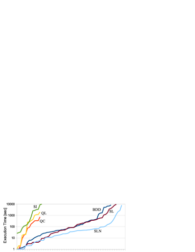
(a) Execution time for amba and genbuf.

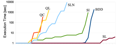
(b) Execution time for add and mult.

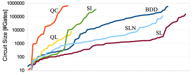
(c) Circuit size for all benchmarks.

Figure 2: Cactus plots summarizing our performance evaluation.

V Conclusion

We compared several SAT- and QBF-based methods to synthesize circuits from strategies, and presented optimizations and efficient implementations for safety specifications. Our SAT-based learning method combines the quantifier elimination approach by Jiang et al. [8] with computational learning as proposed by Ehlers et al. [7], and outperforms BDDs both regarding execution time and circuit size in our experiments.

Future research includes preprocessing for incremental QBF solving, exploiting unreachable states, and parallelization.

Table I contains more performance results. “T” indicates a time-out of $10\,000$ seconds. The suffix $k$ stands for a multiplication with $1000$. The size column $G$ gives the number of AIGER gates defining $T$. The column “files” in QC gives the size of the intermediate files (the QBF trace) produced by QBFCert; we aborted at $20$ GB. “M” indicates that ABC ran out of memory (because QC produces huge circuits). More details can be found in the downloadable archive.

TABLE I: Performance results.

	Size					BDD			QC				QL			SI			SL			SLN
	$|\overline{i}|$	$|\overline{c}|$	$|\overline{x}|$	$G$		time	size		time	size	files		time	size		time	size		time	size		time	size
	[-]	[-]	[-]	[-]		[sec]	[cells]		[sec]	[cells]	[MB]		[sec]	[cells]		[sec]	[cells]		[sec]	[cells]		[sec]	[cells]
add2	4	2	2	17		0.1	2		1	13	0.1		0.1	9		1	9		1	9		0.1	9
add4	8	4	2	45		0.1	4		1	919	0.3		0.1	94		1	28		1	27		0.1	104
add6	12	6	2	73		0.1	6		11	20k	11		3.0	739		1	43		1	45		2	688
add8	16	8	2	101		0.1	8		164	M	738		172	4.0k		2	59		1	63		10	3.6k
add10	20	10	2	129		0.1	10		T	-	$>$17k		T	-		2	79		1	81		76	16k
add12	24	12	2	157		0.1	12		-	-	$>$20k		T	-		3	97		1	99		1.3k	69k
add14	28	14	2	185		0.1	14		-	-	$>$20k		T	-		4	113		1	117		T	-
add16	32	16	2	213		0.1	16		-	-	$>$20k		T	-		4	132		1	135		T	-
add18	36	18	2	241		0.1	18		-	-	$>$20k		T	-		6	151		1	153		T	-
add20	40	20	2	269		0.2	20		-	-	$>$20k		T	-		6	167		1	171		T	-
mult2	4	4	0	24		0.1	4		1	8	0.1		0.1	8		1	8		1	8		0.1	8
mult4	8	8	0	128		0.1	8		1	1.0k	6.1		2	414		3	440		1	95		1	412
mult5	10	10	0	217		0.2	10		12	4.9k	142		27	1.9k		9	2.6k		1	163		7	1.8k
mult6	12	12	0	322		1.1	12		380	23k	2.9k		1.7k	8.2k		57	14k		1	247		40	7.7k
mult7	14	14	0	455		3.2	14		-	-	$>$20k		T	-		962	73k		1	351		411	30k
mult8	16	16	0	604		209	16		-	-	$>$20k		T	-		T	-		1	477		9.2k	122k
mult10	20	20	0	964		T	-		-	-	$>$20k		T	-		T	-		1	777		T	-
mult12	24	24	0	1379		T	-		-	-	$>$20k		T	-		T	-		2	1.2k		T	-
mult16	32	32	0	2450		T	-		-	-	$>$20k		T	-		T	-		4	2.1k		T	-
genbuf1c	5	6	21	134		0.5	1.7k		1	2.9k	2.4		2	95		29	10k		1	101		1	62
genbuf2c	6	7	24	169		1.6	4.8k		9	18k	24.3		20	239		73	25k		3	198		2	119
genbuf3c	7	9	27	202		6.1	11k		86	62k	166		257	709		3.2k	191k		4	301		3	224
genbuf4c	8	10	30	242		12	15k		329	208k	1.3k		2.0k	1.0k		9.9k	222k		14	362		4	326
genbuf5c	9	12	33	284		21	21k		1.4k	M	4.7k		T	-		T	-		43	779		11	455
genbuf6c	10	13	35	323		36	36k		-	-	$>$20k		T	-		T	-		63	781		17	694
genbuf8c	12	15	40	406		282	61k		-	-	$>$20k		T	-		T	-		437	1.0k		44	1.0k
genbuf10c	14	18	45	494		155	100k		-	-	$>$20k		T	-		T	-		206	1.6k		45	1.5k
genbuf12c	16	20	49	561		266	154k		-	-	$>$20k		T	-		T	-		166	1.4k		51	1.1k
genbuf16c	20	24	58	733		465	203k		-	-	$>$20k		T	-		T	-		389	1.5k		47	2.0k
genbuf1b	5	6	23	141		0.8	2.3k		1	3.6k	3.1		1	70		25	11k		1	102		1	62
genbuf2b	6	7	26	174		6.2	6.5k		17	30k	31.7		17	399		111	19k		1	213		1	116
genbuf3b	7	9	30	208		7.8	11k		73	154k	354		252	1.6k		2.5k	202k		3	262		2	217
genbuf4b	8	10	33	245		34	26k		733	666k	2.3k		1.2k	1.2k		3.4k	352k		2	353		2	307
genbuf5b	9	12	37	282		52	29k		T	-	16k		T	-		T	-		5	693		5	863
genbuf6b	10	13	40	322		27	23k		-	-	$>$20k		T	-		T	-		11	1.3k		11	2.2k
genbuf8b	12	15	46	395		61	51k		-	-	$>$20k		T	-		T	-		12	1.1k		6	804
genbuf10b	14	18	53	475		118	80k		-	-	$>$20k		T	-		T	-		25	775		16	1.9k
genbuf12b	16	20	59	547		31	74k		-	-	$>$20k		T	-		T	-		46	1.0k		27	2.0k
genbuf16b	20	24	71	687		44	107k		-	-	$>$20k		T	-		T	-		113	1.3k		113	18k
genbuf1f	5	6	23	138		1.3	2.0k		2	4.8k	2.9		2	67		33	11k		1	74		0.1	54
genbuf2f	6	7	26	168		1.9	6.1k		23	36k	33		20	301		128	27k		1	218		0.1	136
genbuf3f	7	9	30	200		82	12k		169	332k	673		432	1.8k		2.7k	133k		4	372		2	198
genbuf4f	8	10	33	235		15	17k		2.7k	M	6.0k		T	-		T	-		9	762		10	476
genbuf5f	9	12	37	272		47	46k		-	-	$>$20k		T	-		T	-		49	1.6k		18	1.0k
genbuf6f	10	13	40	309		53	42k		-	-	$>$20k		T	-		T	-		185	2.7k		67	1.9k
genbuf7f	11	14	43	344		386	112k		-	-	$>$20k		T	-		T	-		524	3.1k		172	2.5k
amba2c	7	8	28	177		1.3	5.2k		229	516k	985		343	2.3k		294	43k		4	1.2k		6	1.2k
amba3c	9	10	34	237		10	15k		-	-	$>$20k		T	-		8.9k	296k		22	2.3k		12	1.3k
amba4c	11	11	38	279		229	129k		-	-	$>$20k		T	-		T	-		206	18k		93	10k
amba5c	13	13	43	345		1.7k	166k		-	-	$>$20k		T	-		T	-		256	15k		35	3.2k
amba6c	15	14	47	395		5.1k	131k		-	-	$>$20k		T	-		T	-		576	24k		40	3.8k
amba7c	17	15	52	449		6.8k	138k		-	-	$>$20k		T	-		T	-		1.2k	38k		67	4.3k
amba9c	21	18	61	583		T	-		-	-	$>$20k		T	-		T	-		4.1k	86k		151	5.4k
amba10c	23	19	65	630		1.6k	212k		-	-	$>$20k		T	-		T	-		5.6k	110k		218	7.0k
amba2b	7	8	31	189		15	12k		337	584k	1.3k		1.2k	3.7k		739	87k		4	1.3k		6	1.1k
amba3b	9	10	36	231		83	74k		-	-	$>$20k		T	-		T	-		28	3.1k		11	1.4k
amba4b	11	11	42	286		8.3k	314k		-	-	$>$20k		T	-		T	-		602	31k		336	18k
amba5b	13	13	47	344		6.6k	574k		-	-	$>$20k		T	-		T	-		1.1k	41k		45	4.1k
amba6b	15	14	52	391		T	-		-	-	$>$20k		T	-		T	-		3.6k	85k		60	5.7k
amba7b	17	15	57	438		T	-		-	-	$>$20k		T	-		T	-		8.0k	159k		96	6.6k
amba9b	21	18	68	558		T	-		-	-	$>$20k		T	-		T	-		T	-		605	22k
amba10b	23	19	73	606		T	-		-	-	$>$20k		T	-		T	-		T	-		2.7k	72k
amba2f	7	8	31	181		4.1	12k		336	584k	1.4k		1.0k	3.0k		165	30k		3	1.3k		5	1.0k
amba3f	9	10	37	229		101	36k		T	-	$>$16k		T	-		T	-		83	7.0k		52	6.2k
amba4f	11	11	43	282		1.3k	293k		-	-	$>$20k		T	-		T	-		1.7k	44k		1.3k	33k
amba5f	13	13	49	346		T	-		-	-	$>$20k		T	-		T	-		9.5k	104k		2.2k	23k
amba6f	15	14	54	391		T	-		-	-	$>$20k		T	-		T	-		T	-		8.0k	31k

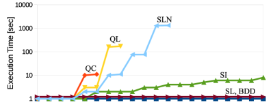
(a) Execution time for add.

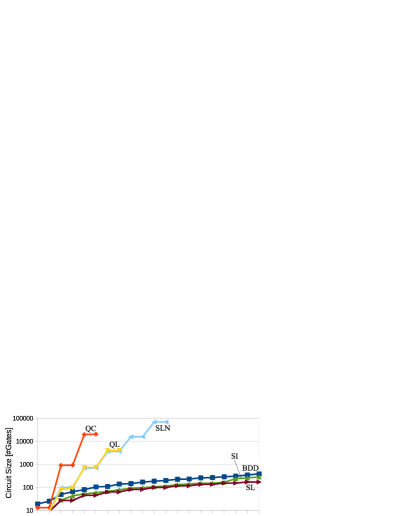
(b) Circuit size for add.

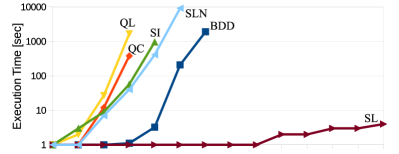
(c) Execution time for mult.

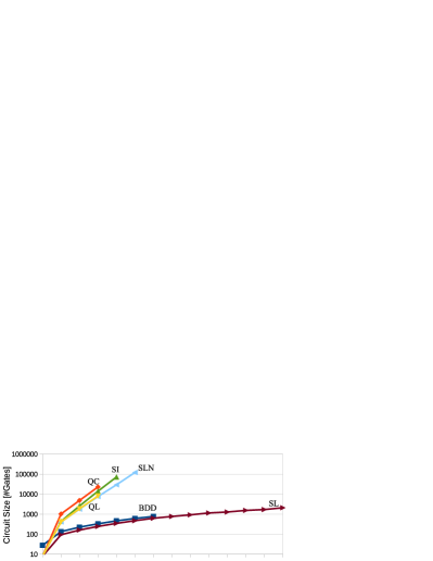
(d) Circuit size for mult.

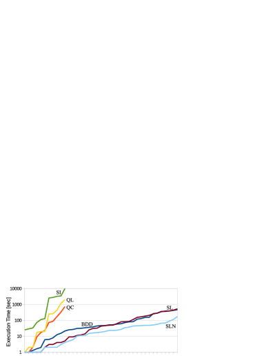
(e) Execution time for genbuf.

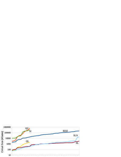
(f) Circuit size for genbuf.

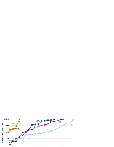
(g) Execution time for amba.

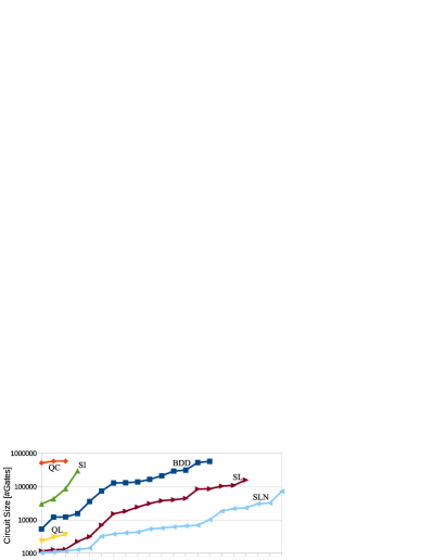
(h) Circuit size for amba.

Figure 3: Cactus plots summarizing execution time and circuit size per benchmark.

Fig. 3 contains cactus plots summarizing the execution time and circuit size per benchmark. For mult, the dependency optimization has an even stronger positive impact than for add, both regarding execution time and circuit size (SL vs. SLN). For genbuf, it results in smaller circuits, but is slower. For amba, it is not beneficial in either metric. The interpolation-based method SI is competitive for add, but has troubles with the other benchmarks. The difference in circuit size can grow very large (more than three orders of magnitude). Our a-posteriori circuit minimization using ABC can only compensate an insignificant fraction of this difference. Investing more effort in post-processing can be expensive, especially for large circuits. We therefore conclude that circuit size is best considered during the synthesis process already. The fact that circuit size and execution time correlate is not surprising. Most of our methods compute circuits for one output signal after the other. The strategy is refined with the circuit for one signal before continuing with the next one. This is necessary in order to prevent uncoordinated choices. If the computed circuits are complicated, then this re-substitution makes the strategy formula for the next output complicated, which results in higher computation times. This may also explain why implementing an interpolation procedure with computational learning is very beneficial (SL vs. SI): computational learning seems to find smaller circuits, and this also pays off in terms of the overall computation time.

References

- [1] A. Biere, M. Heule, H. van Maaren, and T. Walsh, editors. Handbook of Satisfiability. IOS Press, 2009.
- [2] R. Bloem, U. Egly, P. Klampfl, R. Könighofer, and F. Lonsing. SAT-based methods for circuit synthesis. In FMCAD’14, 2014. To appear.
- [3] R. Bloem, S. J. Galler, B. Jobstmann, N. Piterman, A. Pnueli, and M. Weiglhofer. Specify, compile, run: Hardware from PSL. Electr. Notes Theor. Comput. Sci., 190(4):3–16, 2007.
- [4] R. Bloem, R. Könighofer, and M. Seidl. SAT-based synthesis methods for safety specs. In VMCAI’14. Springer, 2014.
- [5] R. K. Brayton and A. Mishchenko. ABC: An academic industrial-strength verification tool. In CAV’10. Springer, 2010.
- [6] V. D’Silva, D. Kroening, M. Purandare, and G. Weissenbacher. Interpolant strength. In VMCAI’10. Springer, 2010.
- [7] R. Ehlers, R. Könighofer, and G. Hofferek. Symbolically synthesizing small circuits. In FMCAD’12. IEEE, 2012.
- [8] J.-H. R. Jiang, H.-P. Lin, and W.-L. Hung. Interpolating functions from large boolean relations. In ICCAD’09. IEEE, 2009.
- [9] B. Jobstmann, S. Staber, A. Griesmayer, and R. Bloem. Finding and fixing faults. J. Comput. Syst. Sci., 78(2):441–460, 2012.
- [10] F. Lonsing and A. Biere. DepQBF: A dependency-aware QBF solver. JSAT, 7(2-3):71–76, 2010.
- [11] F. Lonsing and U. Egly. Incremental QBF solving. In CP’14. Springer, 2014. To appear.
- [12] A. Morgenstern, M. Gesell, and K. Schneider. Solving games using incremental induction. In IFM’13. Springer, 2013.
- [13] A. Niemetz, M. Preiner, F. Lonsing, M. Seidl, and A. Biere. Resolution-based certificate extraction for QBF. In SAT’12. Springer, 2012.
- [14] A. Solar-Lezama. The sketching approach to program synthesis. In APLAS’09. Springer, 2009.