Dilute magnetic topological semiconductors: What’s new beyond the physics of dilute magnetic semiconductors?
Kyoung-Min Kim1 1 1,2
1 2
Abstract
Role of localized magnetic moments in metal-insulator transitions DMFT_RMP c Lee_Nagaosa_Wen_RMP HFQCP_RMP Doped_Si_Review ; Disorder_Review ; Disorder_Interaction_Review DMS_Review TI_Review_I ; TI_Review_II Weyl_Metal_I ; Weyl_Metal_II ; Weyl_Metal_III ; Weyl_Metal_IV Kim_Kim_Sasaki_FMTI ( λ s o , Γ , T ) subscript 𝜆 𝑠 𝑜 Γ 𝑇 (\lambda_{so},\Gamma,T) λ s o subscript 𝜆 𝑠 𝑜 \lambda_{so} T 𝑇 T Γ Γ \Gamma TI_Review_II ; Axion_EM1 ; Axion_EM2 ; Axion_EM3 Disorder_Review ; Disorder_Interaction_Review
An endless effort has been performed to achieve spin polarized electric currents in semiconductors. Dilute magnetic semiconductors had been investigated for more than twenty years DMS_Review RKKY
In this study, we propose the problem of dilute magnetic topological semiconductors, replacing non-topological semiconductors with topological semiconductors. Recently, it has been reported that the evolution of average magnetic correlations from ferromagnetic- to antiferromagnetic- in Fex 2 3 2 3 x ∼ 0.025 similar-to 𝑥 0.025 x\sim 0.025 x ∼ 0.03 similar-to 𝑥 0.03 x\sim 0.03 x ∼ 0.1 similar-to 𝑥 0.1 x\sim 0.1 Kim_Kim_Sasaki_FMTI
Performing the renormalization group analysis for an effective field theory to describe the first occurring “phase transition” within the “ferromagnetic” regime, we find that the variance of the distribution for randomly quenched effective magnetic fields due to ferromagnetic clusters goes toward an infinite fixed point as the concentration of magnetic ions increases. Recalling that time reversal symmetry breaking in this strong spin-orbit coupled system gives rise to the Weyl metallic state Weyl_Metal_I ; Weyl_Metal_II ; Weyl_Metal_III ; Weyl_Metal_IV ( λ s o , Γ , T ) subscript 𝜆 𝑠 𝑜 Γ 𝑇 (\lambda_{so},\Gamma,T) λ s o subscript 𝜆 𝑠 𝑜 \lambda_{so} Γ Γ \Gamma T 𝑇 T ( λ s o c , Γ c ) superscript subscript 𝜆 𝑠 𝑜 𝑐 subscript Γ 𝑐 (\lambda_{so}^{c},\Gamma_{c}) T = 0 𝑇 0 T=0 λ s o c superscript subscript 𝜆 𝑠 𝑜 𝑐 \lambda_{so}^{c} ( λ s o → ∞ , Γ = 0 ) formulae-sequence → subscript 𝜆 𝑠 𝑜 Γ 0 (\lambda_{so}\rightarrow\infty,\Gamma=0) ( λ s o = 0 , Γ = 0 ) formulae-sequence subscript 𝜆 𝑠 𝑜 0 Γ 0 (\lambda_{so}=0,\Gamma=0) TI_BI_QCP Γ c subscript Γ 𝑐 \Gamma_{c} ( λ s o , Γ = 0 ) subscript 𝜆 𝑠 𝑜 Γ
0 (\lambda_{so},\Gamma=0) ( λ s o c , Γ → ∞ ) → superscript subscript 𝜆 𝑠 𝑜 𝑐 Γ
(\lambda_{so}^{c},\Gamma\rightarrow\infty) T = 0 𝑇 0 T=0 Percolation TI_Review_II ; Axion_EM1 ; Axion_EM2 ; Axion_EM3 Disorder_Review DMFT_RMP Disorder_Interaction_Review
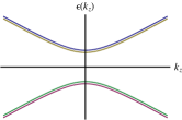
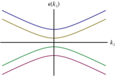
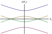
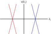
Figure 1: Band structure of the Weyl metallic state. The presence of both time reversal and inversion symmetries gives rise to a degeneracy at each momentum point (First). Applying magnetic fields (𝑯 = H 𝒛 ^ 𝑯 𝐻 bold-^ 𝒛 \bm{H}=H\bm{\hat{z}} m ( | 𝒌 | ) 𝑚 𝒌 m(|\bm{k}|) g H ≪ m ( | 𝒌 | ) much-less-than 𝑔 𝐻 𝑚 𝒌 gH\ll m(|\bm{k}|) g H ≫ m ( | 𝒌 | ) much-greater-than 𝑔 𝐻 𝑚 𝒌 gH\gg m(|\bm{k}|) g 𝑔 g e ´ ´ 𝑒 \acute{e} g − limit-from 𝑔 g- J 𝚽 𝒓 𝐽 subscript 𝚽 𝒓 J\bm{\Phi}_{\bm{r}}
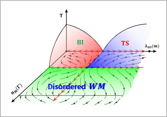
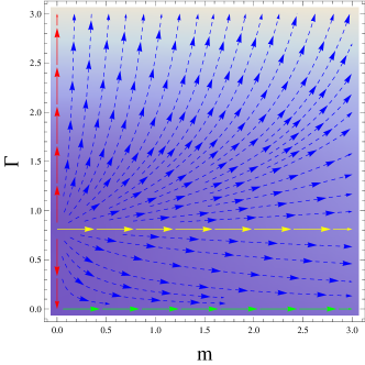
Figure 2: A schematic phase diagram based on the renormalization group analysis for an effective field theory Eq. (3). The 𝒚 − limit-from 𝒚 \bm{y}- λ s o subscript 𝜆 𝑠 𝑜 \lambda_{so} m 𝑚 m 𝒙 − limit-from 𝒙 \bm{x}- Γ Γ \Gamma T 𝑇 T ( λ s o = 0 , Γ = 0 ) formulae-sequence subscript 𝜆 𝑠 𝑜 0 Γ 0 (\lambda_{so}=0,\Gamma=0) ( λ s o → ∞ , Γ = 0 ) formulae-sequence → subscript 𝜆 𝑠 𝑜 Γ 0 (\lambda_{so}\rightarrow\infty,\Gamma=0) ( λ s o c , Γ → ∞ ) → superscript subscript 𝜆 𝑠 𝑜 𝑐 Γ
(\lambda_{so}^{c},\Gamma\rightarrow\infty) ( λ s o c , Γ = 0 ) superscript subscript 𝜆 𝑠 𝑜 𝑐 Γ
0 (\lambda_{so}^{c},\Gamma=0) ( λ s o c , Γ c ) superscript subscript 𝜆 𝑠 𝑜 𝑐 subscript Γ 𝑐 (\lambda_{so}^{c},\Gamma_{c})
The problem of dilute magnetic topological semiconductors differs from that of randomly doped magnetic impurities on the surface state of a topological insulator. One may speculate that half-quantized Hall conductance appears with Anderson localization if doped magnetic ions exhibit ferromagnetic ordering. On the other hand, an anomalous metallic phase can emerge to fall into the universality class of the quantum Hall plateau-plateau transition in the paramagnetic phase although an actual transition occurs between the quantum Hall plateau and the gapless surface state, where Anderson localization may not exist due to the presence of time reversal symmetry in average Fu_Kane_NLsM
We start from an effective-model free energy Axion_EM3
F = − T ∫ − ∞ ∞ d I 𝒓 𝒓 ′ P ( I 𝒓 𝒓 ′ ) ln ∫ D ψ 𝒌 τ D 𝑺 𝒓 τ exp [ − ∫ 0 1 / T d τ ∫ d 3 𝒌 ( 2 π ) 3 ψ σ α † ( 𝒌 , τ ) { ( ∂ τ − μ ) 𝑰 σ σ ′ ⊗ 𝑰 α α ′ \displaystyle F=-T\int_{-\infty}^{\infty}dI_{\bm{r}\bm{r}^{\prime}}P(I_{\bm{r}\bm{r}^{\prime}})\ln\int D\psi_{\bm{k}\tau}D\bm{S}_{\bm{r}\tau}\exp\Bigl{[}-\int_{0}^{1/T}d\tau\int\frac{d^{3}\bm{k}}{(2\pi)^{3}}\psi_{\sigma\alpha}^{\dagger}(\bm{k},\tau)\Bigl{\{}(\partial_{\tau}-\mu)\bm{I}_{\sigma\sigma^{\prime}}\otimes\bm{I}_{\alpha\alpha^{\prime}}
+ v 𝒌 ⋅ 𝝈 σ σ ′ ⊗ 𝝉 α α ′ z + m ( | 𝒌 | ) 𝑰 σ σ ′ ⊗ 𝝉 α α ′ x } ψ σ ′ α ′ ( 𝒌 , τ ) − ∫ 0 1 / T d τ ∫ d 3 𝒓 J ψ σ α † ( 𝒓 , τ ) ( 𝝈 σ σ ′ ⊗ 𝑰 α α ′ ) ψ σ ′ α ′ ( 𝒓 , τ ) ⋅ 𝑺 ( 𝒓 , τ ) \displaystyle+v\bm{k}\cdot\bm{\sigma}_{\sigma\sigma^{\prime}}\otimes\bm{\tau}_{\alpha\alpha^{\prime}}^{z}+m(|\bm{k}|)\bm{I}_{\sigma\sigma^{\prime}}\otimes\bm{\tau}_{\alpha\alpha^{\prime}}^{x}\Bigr{\}}\psi_{\sigma^{\prime}\alpha^{\prime}}(\bm{k},\tau)-\int_{0}^{1/T}d\tau\int d^{3}\bm{r}J\psi_{\sigma\alpha}^{\dagger}(\bm{r},\tau)(\bm{\sigma}_{\sigma\sigma^{\prime}}\otimes\bm{I}_{\alpha\alpha^{\prime}})\psi_{\sigma^{\prime}\alpha^{\prime}}(\bm{r},\tau)\cdot\bm{S}(\bm{r},\tau)
− ∫ 0 1 / T d τ ∫ d 3 𝒓 ∫ d 3 𝒓 ′ I 𝒓 𝒓 ′ 𝑺 ( 𝒓 , τ ) ⋅ 𝑺 ( 𝒓 ′ , τ ) − 𝒮 B ] . \displaystyle-\int_{0}^{1/T}d\tau\int d^{3}\bm{r}\int d^{3}\bm{r}^{\prime}I_{\bm{r}\bm{r}^{\prime}}\bm{S}(\bm{r},\tau)\cdot\bm{S}(\bm{r}^{\prime},\tau)-\mathcal{S}_{B}\Bigr{]}. (1)
Here, ψ σ α ( 𝒌 , τ ) subscript 𝜓 𝜎 𝛼 𝒌 𝜏 \psi_{\sigma\alpha}(\bm{k},\tau) σ 𝜎 \sigma α 𝛼 \alpha 𝝈 σ σ ′ subscript 𝝈 𝜎 superscript 𝜎 ′ \bm{\sigma}_{\sigma\sigma^{\prime}} 𝝉 α α ′ subscript 𝝉 𝛼 superscript 𝛼 ′ \bm{\tau}_{\alpha\alpha^{\prime}} 𝝉 α α ′ z superscript subscript 𝝉 𝛼 superscript 𝛼 ′ 𝑧 \bm{\tau}_{\alpha\alpha^{\prime}}^{z} + + − - m ( | 𝒌 | ) = m − ρ | 𝒌 | 2 𝑚 𝒌 𝑚 𝜌 superscript 𝒌 2 m(|\bm{k}|)=m-\rho|\bm{k}|^{2} sgn ( m ) sgn ( ρ ) > 0 sgn 𝑚 sgn 𝜌 0 \mbox{sgn}(m)\mbox{sgn}(\rho)>0 sgn ( m ) sgn ( ρ ) < 0 sgn 𝑚 sgn 𝜌 0 \mbox{sgn}(m)\mbox{sgn}(\rho)<0 μ 𝜇 \mu 𝑺 ( 𝒓 , τ ) 𝑺 𝒓 𝜏 \bm{S}(\bm{r},\tau) I 𝒓 𝒓 ′ subscript 𝐼 𝒓 superscript 𝒓 ′ I_{\bm{r}\bm{r}^{\prime}} P ( I 𝒓 𝒓 ′ ) 𝑃 subscript 𝐼 𝒓 superscript 𝒓 ′ P(I_{\bm{r}\bm{r}^{\prime}}) J 𝐽 J 𝒮 B subscript 𝒮 𝐵 \mathcal{S}_{B} Spin_Textbook
Hinted from the recent experiment Kim_Kim_Sasaki_FMTI 𝑺 ( 𝒓 , τ ) = 1 2 f σ † ( 𝒓 , τ ) 𝝈 σ σ ′ f σ ′ ( 𝒓 , τ ) 𝑺 𝒓 𝜏 1 2 superscript subscript 𝑓 𝜎 † 𝒓 𝜏 subscript 𝝈 𝜎 superscript 𝜎 ′ subscript 𝑓 superscript 𝜎 ′ 𝒓 𝜏 \bm{S}(\bm{r},\tau)=\frac{1}{2}f_{\sigma}^{\dagger}(\bm{r},\tau)\bm{\sigma}_{\sigma\sigma^{\prime}}f_{\sigma^{\prime}}(\bm{r},\tau) f σ † ( 𝒓 , τ ) f σ ( 𝒓 , τ ) = 1 superscript subscript 𝑓 𝜎 † 𝒓 𝜏 subscript 𝑓 𝜎 𝒓 𝜏 1 f_{\sigma}^{\dagger}(\bm{r},\tau)f_{\sigma}(\bm{r},\tau)=1 Lee_Nagaosa_Wen_RMP
ℱ M F [ 𝚽 𝒓 , χ 𝒓 𝒓 ′ , λ 𝒓 ; μ , T ] = − T ∫ − ∞ ∞ 𝑑 I 𝒓 𝒓 ′ P ( I 𝒓 𝒓 ′ ) ln ∫ D ψ σ α ( 𝒓 , τ ) D f σ ( 𝒓 , τ ) subscript ℱ 𝑀 𝐹 subscript 𝚽 𝒓 subscript 𝜒 𝒓 superscript 𝒓 ′ subscript 𝜆 𝒓 𝜇 𝑇
𝑇 superscript subscript differential-d subscript 𝐼 𝒓 superscript 𝒓 ′ 𝑃 subscript 𝐼 𝒓 superscript 𝒓 ′ 𝐷 subscript 𝜓 𝜎 𝛼 𝒓 𝜏 𝐷 subscript 𝑓 𝜎 𝒓 𝜏 \displaystyle\mathcal{F}_{MF}[\bm{\Phi}_{\bm{r}},\chi_{\bm{r}\bm{r}^{\prime}},\lambda_{\bm{r}};\mu,T]=-T\int_{-\infty}^{\infty}dI_{\bm{r}\bm{r}^{\prime}}P(I_{\bm{r}\bm{r}^{\prime}})\ln\int D\psi_{\sigma\alpha}(\bm{r},\tau)Df_{\sigma}(\bm{r},\tau)
exp [ − ∫ 0 1 / T d τ ∫ d 3 𝒌 ( 2 π ) 3 ψ σ α † ( 𝒌 , τ ) { ( ∂ τ − μ ) 𝑰 σ σ ′ ⊗ 𝑰 α α ′ + v 𝒌 ⋅ 𝝈 σ σ ′ ⊗ 𝝉 α α ′ z + m ( | 𝒌 | ) 𝑰 σ σ ′ ⊗ 𝝉 α α ′ x } ψ σ ′ α ′ ( 𝒌 , τ ) \displaystyle\exp\Bigl{[}-\int_{0}^{1/T}d\tau\int\frac{d^{3}\bm{k}}{(2\pi)^{3}}\psi_{\sigma\alpha}^{\dagger}(\bm{k},\tau)\Bigl{\{}(\partial_{\tau}-\mu)\bm{I}_{\sigma\sigma^{\prime}}\otimes\bm{I}_{\alpha\alpha^{\prime}}+v\bm{k}\cdot\bm{\sigma}_{\sigma\sigma^{\prime}}\otimes\bm{\tau}_{\alpha\alpha^{\prime}}^{z}+m(|\bm{k}|)\bm{I}_{\sigma\sigma^{\prime}}\otimes\bm{\tau}_{\alpha\alpha^{\prime}}^{x}\Bigr{\}}\psi_{\sigma^{\prime}\alpha^{\prime}}(\bm{k},\tau)
− ∫ 0 1 / T d τ ∫ d 3 𝒓 J ψ σ α † ( 𝒓 , τ ) ( 𝝈 σ σ ′ ⊗ 𝑰 α α ′ ) ψ σ ′ α ′ ( 𝒓 , τ ) ⋅ 𝚽 𝒓 − ∫ 0 1 / T d τ ∫ d 3 𝒓 ∫ d 3 𝒓 ′ { f σ † ( 𝒓 , τ ) ( ( ∂ τ + λ 𝒓 ) δ ( 3 ) ( 𝒓 − 𝒓 ′ ) \displaystyle-\int_{0}^{1/T}d\tau\int d^{3}\bm{r}J\psi_{\sigma\alpha}^{\dagger}(\bm{r},\tau)(\bm{\sigma}_{\sigma\sigma^{\prime}}\otimes\bm{I}_{\alpha\alpha^{\prime}})\psi_{\sigma^{\prime}\alpha^{\prime}}(\bm{r},\tau)\cdot\bm{\Phi}_{\bm{r}}-\int_{0}^{1/T}d\tau\int d^{3}\bm{r}\int d^{3}\bm{r}^{\prime}\Bigl{\{}f_{\sigma}^{\dagger}(\bm{r},\tau)\Bigl{(}(\partial_{\tau}+\lambda_{\bm{r}})\delta^{(3)}(\bm{r}-\bm{r}^{\prime})
− I 𝒓 𝒓 ′ χ 𝒓 𝒓 ′ ) f σ ( 𝒓 ′ , τ ) + I 𝒓 𝒓 ′ f σ † ( 𝒓 , τ ) ( 𝚽 𝒓 ′ ⋅ 𝝈 ) σ σ ′ f σ ′ ( 𝒓 , τ ) } − 1 T ∫ d 3 𝒓 ∫ d 3 𝒓 ′ { λ 𝒓 δ ( 3 ) ( 𝒓 − 𝒓 ′ ) + I 𝒓 𝒓 ′ ( χ 𝒓 𝒓 ′ χ 𝒓 ′ 𝒓 \displaystyle-I_{\bm{r}\bm{r}^{\prime}}\chi_{\bm{r}\bm{r}^{\prime}}\Bigr{)}f_{\sigma}(\bm{r}^{\prime},\tau)+I_{\bm{r}\bm{r}^{\prime}}f_{\sigma}^{\dagger}(\bm{r},\tau)(\bm{\Phi}_{\bm{r}^{\prime}}\cdot\bm{\sigma})_{\sigma\sigma^{\prime}}f_{\sigma^{\prime}}(\bm{r},\tau)\Bigr{\}}-\frac{1}{T}\int d^{3}\bm{r}\int d^{3}\bm{r}^{\prime}\Bigl{\{}\lambda_{\bm{r}}\delta^{(3)}(\bm{r}-\bm{r}^{\prime})+I_{\bm{r}\bm{r}^{\prime}}(\chi_{\bm{r}\bm{r}^{\prime}}\chi_{\bm{r}^{\prime}\bm{r}}
− 𝚽 𝒓 ⋅ 𝚽 𝒓 ′ ) } ] , \displaystyle-\bm{\Phi}_{\bm{r}}\cdot\bm{\Phi}_{\bm{r}^{\prime}})\Bigr{\}}\Bigr{]}, (2)
where 𝚽 𝒓 subscript 𝚽 𝒓 \bm{\Phi}_{\bm{r}} χ 𝒓 𝒓 ′ subscript 𝜒 𝒓 superscript 𝒓 ′ \chi_{\bm{r}\bm{r}^{\prime}} λ 𝒓 subscript 𝜆 𝒓 \lambda_{\bm{r}} I 𝒓 𝒓 ′ subscript 𝐼 𝒓 superscript 𝒓 ′ I_{\bm{r}\bm{r}^{\prime}}
Our scenario is as follows. A control parameter is ⟨ I 𝒓 𝒓 ′ ⟩ = ∫ − ∞ ∞ 𝑑 I 𝒓 𝒓 ′ P ( I 𝒓 𝒓 ′ ) I 𝒓 𝒓 ′ delimited-⟨⟩ subscript 𝐼 𝒓 superscript 𝒓 ′ superscript subscript differential-d subscript 𝐼 𝒓 superscript 𝒓 ′ 𝑃 subscript 𝐼 𝒓 superscript 𝒓 ′ subscript 𝐼 𝒓 superscript 𝒓 ′ \langle I_{\bm{r}\bm{r}^{\prime}}\rangle=\int_{-\infty}^{\infty}dI_{\bm{r}\bm{r}^{\prime}}P(I_{\bm{r}\bm{r}^{\prime}})I_{\bm{r}\bm{r}^{\prime}} sgn ⟨ I 𝒓 𝒓 ′ ⟩ < 0 sgn delimited-⟨⟩ subscript 𝐼 𝒓 superscript 𝒓 ′ 0 \mbox{sgn}\langle I_{\bm{r}\bm{r}^{\prime}}\rangle<0 ⟨ χ 𝒓 𝒓 ′ ⟩ = ∫ − ∞ ∞ 𝑑 I 𝒓 𝒓 ′ P ( I 𝒓 𝒓 ′ ) χ 𝒓 𝒓 ′ = 0 delimited-⟨⟩ subscript 𝜒 𝒓 superscript 𝒓 ′ superscript subscript differential-d subscript 𝐼 𝒓 superscript 𝒓 ′ 𝑃 subscript 𝐼 𝒓 superscript 𝒓 ′ subscript 𝜒 𝒓 superscript 𝒓 ′ 0 \langle\chi_{\bm{r}\bm{r}^{\prime}}\rangle=\int_{-\infty}^{\infty}dI_{\bm{r}\bm{r}^{\prime}}P(I_{\bm{r}\bm{r}^{\prime}})\chi_{\bm{r}\bm{r}^{\prime}}=0 ⟨ 𝚽 𝒓 ⟩ = L − 3 ∫ d 3 𝒓 ′ ∫ − ∞ ∞ 𝑑 I 𝒓 𝒓 ′ P ( I 𝒓 𝒓 ′ ) 𝚽 𝒓 ′ = 0 delimited-⟨⟩ subscript 𝚽 𝒓 superscript 𝐿 3 superscript 𝑑 3 superscript 𝒓 ′ superscript subscript differential-d subscript 𝐼 𝒓 superscript 𝒓 ′ 𝑃 subscript 𝐼 𝒓 superscript 𝒓 ′ subscript 𝚽 superscript 𝒓 ′ 0 \langle\bm{\Phi}_{\bm{r}}\rangle=L^{-3}\int d^{3}\bm{r}^{\prime}\int_{-\infty}^{\infty}dI_{\bm{r}\bm{r}^{\prime}}P(I_{\bm{r}\bm{r}^{\prime}})\bm{\Phi}_{\bm{r}^{\prime}}=0 L − 3 ∫ d 3 𝒓 L − 3 ∫ d 3 𝒓 ′ ⟨ 𝚽 𝒓 ⋅ 𝚽 𝒓 ′ ⟩ = L − 3 ∫ d 3 𝒓 L − 3 ∫ d 3 𝒓 ′ ∫ − ∞ ∞ 𝑑 I 𝒓 𝒓 ′ P ( I 𝒓 𝒓 ′ ) 𝚽 𝒓 ⋅ 𝚽 𝒓 ′ ∝ T − η 𝚽 superscript 𝐿 3 superscript 𝑑 3 𝒓 superscript 𝐿 3 superscript 𝑑 3 superscript 𝒓 ′ delimited-⟨⟩ ⋅ subscript 𝚽 𝒓 subscript 𝚽 superscript 𝒓 ′ superscript 𝐿 3 superscript 𝑑 3 𝒓 superscript 𝐿 3 superscript 𝑑 3 superscript 𝒓 ′ superscript subscript ⋅ differential-d subscript 𝐼 𝒓 superscript 𝒓 ′ 𝑃 subscript 𝐼 𝒓 superscript 𝒓 ′ subscript 𝚽 𝒓 subscript 𝚽 superscript 𝒓 ′ proportional-to superscript 𝑇 subscript 𝜂 𝚽 L^{-3}\int d^{3}\bm{r}L^{-3}\int d^{3}\bm{r}^{\prime}\langle\bm{\Phi}_{\bm{r}}\cdot\bm{\Phi}_{\bm{r}^{\prime}}\rangle=L^{-3}\int d^{3}\bm{r}L^{-3}\int d^{3}\bm{r}^{\prime}\int_{-\infty}^{\infty}dI_{\bm{r}\bm{r}^{\prime}}P(I_{\bm{r}\bm{r}^{\prime}})\bm{\Phi}_{\bm{r}}\cdot\bm{\Phi}_{\bm{r}^{\prime}}\propto T^{-\eta_{\bm{\Phi}}} sgn ⟨ I 𝒓 𝒓 ′ ⟩ > 0 sgn delimited-⟨⟩ subscript 𝐼 𝒓 superscript 𝒓 ′ 0 \mbox{sgn}\langle I_{\bm{r}\bm{r}^{\prime}}\rangle>0 ⟨ 𝚽 𝒓 ⟩ = L − 3 ∫ d 3 𝒓 ′ ∫ − ∞ ∞ 𝑑 I 𝒓 𝒓 ′ P ( I 𝒓 𝒓 ′ ) 𝚽 𝒓 ′ = 0 delimited-⟨⟩ subscript 𝚽 𝒓 superscript 𝐿 3 superscript 𝑑 3 superscript 𝒓 ′ superscript subscript differential-d subscript 𝐼 𝒓 superscript 𝒓 ′ 𝑃 subscript 𝐼 𝒓 superscript 𝒓 ′ subscript 𝚽 superscript 𝒓 ′ 0 \langle\bm{\Phi}_{\bm{r}}\rangle=L^{-3}\int d^{3}\bm{r}^{\prime}\int_{-\infty}^{\infty}dI_{\bm{r}\bm{r}^{\prime}}P(I_{\bm{r}\bm{r}^{\prime}})\bm{\Phi}_{\bm{r}^{\prime}}=0 ⟨ χ 𝒓 𝒓 ′ ⟩ = ∫ − ∞ ∞ 𝑑 I 𝒓 𝒓 ′ P ( I 𝒓 𝒓 ′ ) χ 𝒓 𝒓 ′ = 0 delimited-⟨⟩ subscript 𝜒 𝒓 superscript 𝒓 ′ superscript subscript differential-d subscript 𝐼 𝒓 superscript 𝒓 ′ 𝑃 subscript 𝐼 𝒓 superscript 𝒓 ′ subscript 𝜒 𝒓 superscript 𝒓 ′ 0 \langle\chi_{\bm{r}\bm{r}^{\prime}}\rangle=\int_{-\infty}^{\infty}dI_{\bm{r}\bm{r}^{\prime}}P(I_{\bm{r}\bm{r}^{\prime}})\chi_{\bm{r}\bm{r}^{\prime}}=0 L − 3 ∫ d 3 𝒓 L − 3 ∫ d 3 𝒓 ′ L − 3 ∫ d 3 𝒓 1 L − 3 ∫ d 3 𝒓 1 ′ ⟨ χ 𝒓 𝒓 ′ χ 𝒓 1 𝒓 1 ′ ⟩ ∝ T − η χ proportional-to superscript 𝐿 3 superscript 𝑑 3 𝒓 superscript 𝐿 3 superscript 𝑑 3 superscript 𝒓 ′ superscript 𝐿 3 superscript 𝑑 3 subscript 𝒓 1 superscript 𝐿 3 superscript 𝑑 3 superscript subscript 𝒓 1 ′ delimited-⟨⟩ subscript 𝜒 𝒓 superscript 𝒓 ′ subscript 𝜒 subscript 𝒓 1 superscript subscript 𝒓 1 ′ superscript 𝑇 subscript 𝜂 𝜒 L^{-3}\int d^{3}\bm{r}L^{-3}\int d^{3}\bm{r}^{\prime}L^{-3}\int d^{3}\bm{r}_{1}L^{-3}\int d^{3}\bm{r}_{1}^{\prime}\langle\chi_{\bm{r}\bm{r}^{\prime}}\chi_{\bm{r}_{1}\bm{r}_{1}^{\prime}}\rangle\propto T^{-\eta_{\chi}} L 𝐿 L
This magnetic evolution gives rise to the variation in transport properties as discussed in the introduction. In particular, normal metallic transport properties in magnetoresistivity and Hall effect appear from topological semiconducting transport behaviors in the ferromagnetic-in-average region before the antiferromagnetic-in-average region. According to the above physical picture, randomly frozen magnetic clusters described by 𝚽 𝒓 subscript 𝚽 𝒓 \bm{\Phi}_{\bm{r}} E 𝒓 ( 𝒌 ) = − μ ± v 2 ( k x 2 + k y 2 ) + ( J | 𝚽 𝒓 | ± m 2 ( | 𝒌 | ) + v 2 k z 2 ) 2 subscript 𝐸 𝒓 𝒌 plus-or-minus 𝜇 superscript 𝑣 2 superscript subscript 𝑘 𝑥 2 superscript subscript 𝑘 𝑦 2 superscript plus-or-minus 𝐽 subscript 𝚽 𝒓 superscript 𝑚 2 𝒌 superscript 𝑣 2 superscript subscript 𝑘 𝑧 2 2 E_{\bm{r}}(\bm{k})=-\mu\pm\sqrt{v^{2}(k_{x}^{2}+k_{y}^{2})+(J|\bm{\Phi}_{\bm{r}}|\pm\sqrt{m^{2}(|\bm{k}|)+v^{2}k_{z}^{2}})^{2}} 𝒓 𝒓 \bm{r} J | 𝚽 𝒓 | > | m ( | 𝒌 | ) | 𝐽 subscript 𝚽 𝒓 𝑚 𝒌 J|\bm{\Phi}_{\bm{r}}|>|m(|\bm{k}|)| 𝒓 𝒓 \bm{r}
In order to understand the nature of such inhomogeneous mixtures, we construct an effective field theory based on the above physical picture. It is straightforward to show that randomly quenched effective magnetic fields (J 𝚽 𝒓 𝐽 subscript 𝚽 𝒓 J\bm{\Phi}_{\bm{r}} 𝒄 𝒄 \bm{c} P ( I 𝒓 𝒓 ′ ) 𝑃 subscript 𝐼 𝒓 superscript 𝒓 ′ P(I_{\bm{r}\bm{r}^{\prime}}) P ( 𝚽 𝒓 ) 𝑃 subscript 𝚽 𝒓 P(\bm{\Phi}_{\bm{r}}) 𝚽 𝒓 [ I 𝒓 𝒓 ′ ] subscript 𝚽 𝒓 delimited-[] subscript 𝐼 𝒓 superscript 𝒓 ′ \bm{\Phi}_{\bm{r}}[I_{\bm{r}\bm{r}^{\prime}}] Kettemann Quantum_Griffiths
We start from an effective Dirac theory with random chiral gauge fields, S = ∫ d 4 x ψ ¯ ( i γ μ ∂ μ − m + γ μ γ 5 c μ ) ψ 𝑆 superscript 𝑑 4 𝑥 ¯ 𝜓 𝑖 superscript 𝛾 𝜇 subscript 𝜇 𝑚 superscript 𝛾 𝜇 superscript 𝛾 5 subscript 𝑐 𝜇 𝜓 S=\int d^{4}x\bar{\psi}(i\gamma^{\mu}\partial_{\mu}-m+\gamma^{\mu}\gamma^{5}c_{\mu})\psi c μ subscript 𝑐 𝜇 c_{\mu} Γ Γ \Gamma Disorder_Review 𝒮 B = 𝒮 R + 𝒮 C T subscript 𝒮 𝐵 subscript 𝒮 𝑅 subscript 𝒮 𝐶 𝑇 \mathcal{S}_{B}=\mathcal{S}_{R}+\mathcal{S}_{CT}
𝒮 R subscript 𝒮 𝑅 \displaystyle\mathcal{S}_{R} = \displaystyle= ∫ 0 β d τ ∫ d d − 1 𝒓 { ψ ¯ R a ( 𝒓 , τ ) ( i γ τ ∂ τ + i v R 𝜸 ⋅ ∇ − m R ) ψ R a ( 𝒓 , τ ) \displaystyle\int_{0}^{\beta}d\tau\int d^{d-1}\bm{r}\Bigl{\{}\bar{\psi}_{R}^{a}(\bm{r},\tau)(i\gamma^{\tau}\partial_{\tau}+iv_{R}\bm{\gamma}\cdot\bm{\nabla}-m_{R})\psi_{R}^{a}(\bm{r},\tau)
+ \displaystyle+ Γ R 2 ∫ 0 β d τ ′ ψ ¯ R a ( 𝒓 , τ ) γ μ γ 5 ψ R a ( 𝒓 , τ ) ψ ¯ R a ′ ( 𝒓 , τ ′ ) γ μ γ 5 ψ R a ′ ( 𝒓 , τ ′ ) } , \displaystyle\frac{\Gamma_{R}}{2}\int_{0}^{\beta}d\tau^{\prime}\bar{\psi}_{R}^{a}(\bm{r},\tau)\gamma^{\mu}\gamma^{5}\psi_{R}^{a}(\bm{r},\tau)\bar{\psi}_{R}^{a^{\prime}}(\bm{r},\tau^{\prime})\gamma_{\mu}\gamma^{5}\psi_{R}^{a^{\prime}}(\bm{r},\tau^{\prime})\Bigr{\}},
𝒮 C T subscript 𝒮 𝐶 𝑇 \displaystyle\mathcal{S}_{CT} = \displaystyle= ∫ 0 β d τ ∫ d d − 1 𝒓 { ψ ¯ R a ( 𝒓 , τ ) ( δ ψ ω i γ τ ∂ τ + δ ψ 𝒌 i v R 𝜸 ⋅ ∇ − δ m m R ) ψ R a ( 𝒓 , τ ) \displaystyle\int_{0}^{\beta}d\tau\int d^{d-1}\bm{r}\Bigl{\{}\bar{\psi}_{R}^{a}(\bm{r},\tau)(\delta_{\psi}^{\omega}i\gamma^{\tau}\partial_{\tau}+\delta_{\psi}^{\bm{k}}iv_{R}\bm{\gamma}\cdot\bm{\nabla}-\delta_{m}m_{R})\psi_{R}^{a}(\bm{r},\tau) (3)
+ \displaystyle+ δ Γ Γ R 2 ∫ 0 β d τ ′ ψ ¯ R a ( 𝒓 , τ ) γ μ γ 5 ψ R a ( 𝒓 , τ ) ψ ¯ R a ′ ( 𝒓 , τ ′ ) γ μ γ 5 ψ R a ′ ( 𝒓 , τ ′ ) } \displaystyle\delta_{\Gamma}\frac{\Gamma_{R}}{2}\int_{0}^{\beta}d\tau^{\prime}\bar{\psi}_{R}^{a}(\bm{r},\tau)\gamma^{\mu}\gamma^{5}\psi_{R}^{a}(\bm{r},\tau)\bar{\psi}_{R}^{a^{\prime}}(\bm{r},\tau^{\prime})\gamma_{\mu}\gamma^{5}\psi_{R}^{a^{\prime}}(\bm{r},\tau^{\prime})\Bigr{\}}
Here, ψ R a ( 𝒓 , τ ) superscript subscript 𝜓 𝑅 𝑎 𝒓 𝜏 {\psi}_{R}^{a}(\bm{r},\tau) a = 1 , … , R 𝑎 1 … 𝑅
a=1,...,R v R subscript 𝑣 𝑅 v_{R} m R subscript 𝑚 𝑅 m_{R} Γ R subscript Γ 𝑅 \Gamma_{R} δ ψ ω superscript subscript 𝛿 𝜓 𝜔 \delta_{\psi}^{\omega} δ ψ 𝒌 superscript subscript 𝛿 𝜓 𝒌 \delta_{\psi}^{\bm{k}} δ m subscript 𝛿 𝑚 \delta_{m} δ Γ subscript 𝛿 Γ \delta_{\Gamma}
ψ B a ( 𝒓 , τ ) = Z ψ ω 1 2 ψ R a ( 𝒓 , τ ) , v B = Z ψ 𝒌 Z ψ ω − 1 v R , formulae-sequence superscript subscript 𝜓 𝐵 𝑎 𝒓 𝜏 superscript superscript subscript 𝑍 𝜓 𝜔 1 2 superscript subscript 𝜓 𝑅 𝑎 𝒓 𝜏 subscript 𝑣 𝐵 superscript subscript 𝑍 𝜓 𝒌 superscript superscript subscript 𝑍 𝜓 𝜔 1 subscript 𝑣 𝑅 \displaystyle\psi_{B}^{a}(\bm{r},\tau)={Z_{\psi}^{\omega}}^{\frac{1}{2}}\psi_{R}^{a}(\bm{r},\tau),~{}~{}~{}v_{B}=Z_{\psi}^{\bm{k}}{Z_{\psi}^{\omega}}^{-1}v_{R},
m B = Z m Z ψ ω − 1 m R , Γ B = μ ε Z Γ Z ψ ω − 2 Γ R , formulae-sequence subscript 𝑚 𝐵 subscript 𝑍 𝑚 superscript superscript subscript 𝑍 𝜓 𝜔 1 subscript 𝑚 𝑅 subscript Γ 𝐵 superscript 𝜇 𝜀 subscript 𝑍 Γ superscript superscript subscript 𝑍 𝜓 𝜔 2 subscript Γ 𝑅 \displaystyle m_{B}=Z_{m}{Z_{\psi}^{\omega}}^{-1}m_{R},~{}~{}~{}\Gamma_{B}=\mu^{\varepsilon}Z_{\Gamma}{Z_{\psi}^{\omega}}^{-2}\Gamma_{R}, (4)
where renormalization constants are given by
Z ψ ω = 1 + δ ψ ω , Z ψ 𝒌 = 1 + δ ψ 𝒌 , formulae-sequence superscript subscript 𝑍 𝜓 𝜔 1 superscript subscript 𝛿 𝜓 𝜔 superscript subscript 𝑍 𝜓 𝒌 1 superscript subscript 𝛿 𝜓 𝒌 \displaystyle Z_{\psi}^{\omega}=1+\delta_{\psi}^{\omega},~{}~{}~{}Z_{\psi}^{\bm{k}}=1+\delta_{\psi}^{\bm{k}},
Z m = 1 + δ m , Z Γ = 1 + δ Γ . formulae-sequence subscript 𝑍 𝑚 1 subscript 𝛿 𝑚 subscript 𝑍 Γ 1 subscript 𝛿 Γ \displaystyle Z_{m}=1+\delta_{m},~{}~{}~{}Z_{\Gamma}=1+\delta_{\Gamma}. (5)
Here, μ 𝜇 \mu ε = d − 3 𝜀 𝑑 3 \varepsilon=d-3
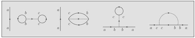
Performing the standard procedure for the renormalization group analysis, we find renormalization group equations, where both vertex and self-energy corrections are introduced self-consistently. See Fig. 3, where all quantum corrections are shown as Feynman’s diagrams up to the one-loop order for vertex corrections and the two-loop order for self-energy corrections. All details are shown in our supplementary material. Here, we point out that the renormalization constant of the “interaction” vertex remains to be Z Γ = 1 subscript 𝑍 Γ 1 Z_{\Gamma}=1 Γ R → ∞ → subscript Γ 𝑅 \Gamma_{R}\rightarrow\infty m R → 0 → subscript 𝑚 𝑅 0 m_{R}\rightarrow 0
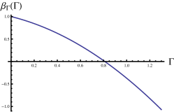
d ln Γ R d ln μ = 1 − a Γ Γ R − b Γ Γ R 2 , 𝑑 subscript Γ 𝑅 𝑑 𝜇 1 subscript 𝑎 Γ subscript Γ 𝑅 subscript 𝑏 Γ superscript subscript Γ 𝑅 2 \displaystyle\frac{d\ln\Gamma_{R}}{d\ln\mu}=1-a_{\Gamma}\Gamma_{R}-b_{\Gamma}\Gamma_{R}^{2},
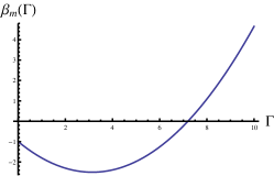
d ln m R d ln μ = − 1 − a m Γ R + b m Γ R 2 , 𝑑 subscript 𝑚 𝑅 𝑑 𝜇 1 subscript 𝑎 𝑚 subscript Γ 𝑅 subscript 𝑏 𝑚 superscript subscript Γ 𝑅 2 \displaystyle\frac{d\ln m_{R}}{d\ln\mu}=-1-a_{m}\Gamma_{R}+b_{m}\Gamma_{R}^{2}, (6)
where positive numerical constants are given by a Γ = 2 π subscript 𝑎 Γ 2 𝜋 a_{\Gamma}=\frac{2}{\pi} b Γ = 29 4 π 2 subscript 𝑏 Γ 29 4 superscript 𝜋 2 b_{\Gamma}=\frac{29}{4\pi^{2}} a m = 3 π subscript 𝑎 𝑚 3 𝜋 a_{m}=\frac{3}{\pi} b m = 3 2 π 2 subscript 𝑏 𝑚 3 2 superscript 𝜋 2 b_{m}=\frac{3}{2\pi^{2}} m R = 0 subscript 𝑚 𝑅 0 m_{R}=0 Γ R = Γ c subscript Γ 𝑅 subscript Γ 𝑐 \Gamma_{R}=\Gamma_{c} Γ R = 0 subscript Γ 𝑅 0 \Gamma_{R}=0 Γ R → ∞ → subscript Γ 𝑅 \Gamma_{R}\rightarrow\infty Lee_Nagaosa_Wen_RMP ( m R → 0 , Γ R → ∞ ) formulae-sequence → subscript 𝑚 𝑅 0 → subscript Γ 𝑅 (m_{R}\rightarrow 0,\Gamma_{R}\rightarrow\infty) ( m R → ∞ , Γ R → 0 ) formulae-sequence → subscript 𝑚 𝑅 → subscript Γ 𝑅 0 (m_{R}\rightarrow\infty,\Gamma_{R}\rightarrow 0) ( m R → − ∞ , Γ R → ∞ ) formulae-sequence → subscript 𝑚 𝑅 → subscript Γ 𝑅 (m_{R}\rightarrow-\infty,\Gamma_{R}\rightarrow\infty) Anderson_Mott
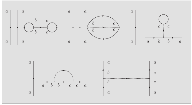
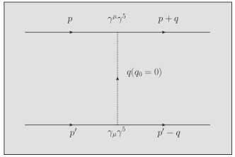
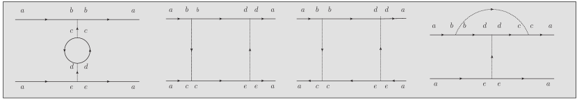
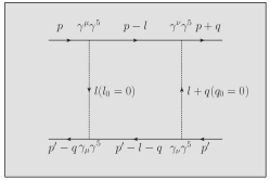
Figure 3: Feynman’s diagrams up to the one-loop order for vertex corrections and the two-loop order for self-energy corrections. First of all, we point out that quantum corrections including fermion loops vanish in the replica limit of N R → 0 → subscript 𝑁 𝑅 0 N_{R}\rightarrow 0 1 / ε 1 𝜀 1/\varepsilon Z Γ = 1 subscript 𝑍 Γ 1 Z_{\Gamma}=1 1 / ε 1 𝜀 1/\varepsilon Z ψ ω superscript subscript 𝑍 𝜓 𝜔 Z_{\psi}^{\omega} b m subscript 𝑏 𝑚 b_{m}
One may understand the emergence of this novel metallic fixed point as follows. First of all, Γ R → ∞ → subscript Γ 𝑅 \Gamma_{R}\rightarrow\infty m R → ± ∞ → subscript 𝑚 𝑅 plus-or-minus m_{R}\rightarrow\pm\infty Γ R → ∞ → subscript Γ 𝑅 \Gamma_{R}\rightarrow\infty Γ R ≫ m R much-greater-than subscript Γ 𝑅 subscript 𝑚 𝑅 \Gamma_{R}\gg m_{R} ( m R → ± ∞ , Γ R → ∞ ) formulae-sequence → subscript 𝑚 𝑅 plus-or-minus → subscript Γ 𝑅 (m_{R}\rightarrow\pm\infty,\Gamma_{R}\rightarrow\infty) ( m R → ∞ , Γ R = 0 ) formulae-sequence → subscript 𝑚 𝑅 subscript Γ 𝑅 0 (m_{R}\rightarrow\infty,\Gamma_{R}=0) ( m R → ∞ , Γ R → ∞ ) formulae-sequence → subscript 𝑚 𝑅 → subscript Γ 𝑅 (m_{R}\rightarrow\infty,\Gamma_{R}\rightarrow\infty) b m subscript 𝑏 𝑚 b_{m} Disorder_Review ( m R → ± ∞ , Γ R = 0 ) formulae-sequence → subscript 𝑚 𝑅 plus-or-minus subscript Γ 𝑅 0 (m_{R}\rightarrow\pm\infty,\Gamma_{R}=0) ( m R = 0 , Γ R → ∞ ) formulae-sequence subscript 𝑚 𝑅 0 → subscript Γ 𝑅 (m_{R}=0,\Gamma_{R}\rightarrow\infty)
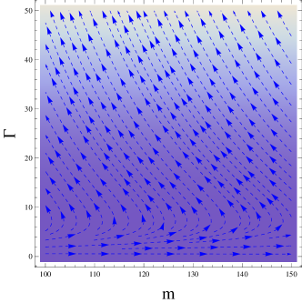
Figure 4: Renormalization group flow as the solution of the coupled renormalization group equations (6). A characteristic feature is the emergence of a novel stable fixed point ( m R = 0 , Γ R → ∞ ) formulae-sequence subscript 𝑚 𝑅 0 → subscript Γ 𝑅 (m_{R}=0,\Gamma_{R}\rightarrow\infty) ( m R = 0 , Γ R = 0 ) formulae-sequence subscript 𝑚 𝑅 0 subscript Γ 𝑅 0 (m_{R}=0,\Gamma_{R}=0) ( m R = 0 , Γ R → ∞ ) formulae-sequence subscript 𝑚 𝑅 0 → subscript Γ 𝑅 (m_{R}=0,\Gamma_{R}\rightarrow\infty) ( m R = 0 , Γ R = Γ c ) formulae-sequence subscript 𝑚 𝑅 0 subscript Γ 𝑅 subscript Γ 𝑐 (m_{R}=0,\Gamma_{R}=\Gamma_{c}) ( m R → ∞ , Γ R = 0 ) formulae-sequence → subscript 𝑚 𝑅 subscript Γ 𝑅 0 (m_{R}\rightarrow\infty,\Gamma_{R}=0) ( m R → − ∞ , Γ R = 0 ) formulae-sequence → subscript 𝑚 𝑅 subscript Γ 𝑅 0 (m_{R}\rightarrow-\infty,\Gamma_{R}=0)
We speculate what would happen when the chemical potential lies above the band gap, resulting in a Fermi surface. First of all, the presence of the Fermi surface changes the engineering dimension of the variance Γ R subscript Γ 𝑅 \Gamma_{R} + 1 1 +1 − 1 1 -1
d ln Γ R d ln μ = − 1 − c Γ R , 𝑑 subscript Γ 𝑅 𝑑 𝜇 1 𝑐 subscript Γ 𝑅 \displaystyle\frac{d\ln\Gamma_{R}}{d\ln\mu}=-1-c\Gamma_{R},
where c 𝑐 c Γ R → ∞ → subscript Γ 𝑅 \Gamma_{R}\rightarrow\infty m R = 0 subscript 𝑚 𝑅 0 m_{R}=0 Weyl_Metal_I ; Weyl_Metal_IV ; Axion_EM2 ; Axion_EM3
Although we expect that this infinite variance fixed point should exhibit the strong inhomogeneity, its thermodynamic nature looks much complicated, where randomly distributed ferromagnetic clusters would interact with each other beyond our present description. Then, quantum Griffiths phenomena Quantum_Griffiths
We believe that this infinite randomness fixed point can be verified by atomic force microscopy. Although the local electronic spectrum will not show strong inhomogeneity around zero bias in the metallic regime, it should be observed deep inside the spectrum around − μ 𝜇 -\mu μ 𝜇 \mu
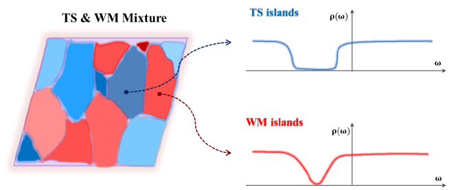
Figure 5: A schematic picture for the local density of states probed by atomic force microscopy. Consider the case when the chemical potential lies above the band gap, which corresponds to a metallic state. Recalling that the infinite variance fixed point is identified with inhomogeneous mixtures between a normal Fermi surface with degeneracy in a Dirac spectrum and a pair of chiral Fermi surfaces without degeneracy in a pair of Weyl spectrum, we predict that a gap feature appears in a certain region which corresponds to the region of small ferromagnetic clusters while a v-shaped pseudogap feature results at a different position which coincides with the region of large ferromagnetic clusters exceeding the band gap.
In summary, we proposed the problem of dilute magnetic topological semiconductors, novel physics of which beyond that of dilute magnetic semiconductors is the emergence of randomly distributed Weyl metallic islands. Performing the renormalization group analysis for an effective Dirac theory with random chiral gauge fluctuations, expected to encode the information of randomly quenched magnetic moments, we find that the variance of random chiral gauge fields reaches an infinite fixed point as long as average magnetic correlations remain to be ferromagnetic, which enforces the mass gap to vanish. As a result, we find a disorder driven novel metallic phase and an associated insulator-metal phase transition beyond either the Anderson or the Mott metal-insulator transition, where this metallic state appears to be identified with the infinite variance fixed point. Recalling that quantum Griffiths phenomena may arise in the vicinity of this infinite variance fixed point, we predicted continuous nonuniversal changes in the temperature exponent of the uniform spin susceptibility. In addition, we claimed that this picture of inhomogeneous mixtures can be verified by atomic force microscopy. However, a difficult fundamental problem remains, that is, how to understand transport coefficients near this infinite variance fixed point, where random axion electrodynamics arises to govern electromagnetic properties, identified with the problem of dilute magnetic topological semiconductors.
Acknowledgement
This study was supported by the Ministry of Education, Science, and Technology (No. 2012R1A1B3000550 and No. 2011-0030785) of the National Research Foundation of Korea (NRF) and by TJ Park Science Fellowship of the POSCO TJ Park Foundation.
Appendix A From effective magnetic fields to chiral gauge fields
The kinetic-energy sector for dynamics of bulk electrons can be rewritten as the standard representation of the Dirac theory in the following way
S [ ψ † , ψ ] 𝑆 superscript 𝜓 † 𝜓 \displaystyle S[\psi^{\dagger},\psi] = \displaystyle= ∫ 0 β 𝑑 τ ∫ d 3 𝒌 ( 2 π ) 3 ψ σ α † ( 𝒌 , τ ) { ∂ τ 𝑰 σ σ ′ ⊗ 𝑰 α α ′ + v F 𝒌 ⋅ 𝝈 σ σ ′ ⊗ 𝝉 α α ′ z + m ( | 𝒌 | ) 𝑰 σ σ ′ ⊗ 𝝉 α α ′ x } ψ σ ′ α ′ ( 𝒌 , τ ) superscript subscript 0 𝛽 differential-d 𝜏 superscript 𝑑 3 𝒌 superscript 2 𝜋 3 superscript subscript 𝜓 𝜎 𝛼 † 𝒌 𝜏 subscript 𝜏 tensor-product subscript 𝑰 𝜎 superscript 𝜎 ′ subscript 𝑰 𝛼 superscript 𝛼 ′ tensor-product ⋅ subscript 𝑣 𝐹 𝒌 subscript 𝝈 𝜎 superscript 𝜎 ′ superscript subscript 𝝉 𝛼 superscript 𝛼 ′ 𝑧 tensor-product 𝑚 𝒌 subscript 𝑰 𝜎 superscript 𝜎 ′ superscript subscript 𝝉 𝛼 superscript 𝛼 ′ 𝑥 subscript 𝜓 superscript 𝜎 ′ superscript 𝛼 ′ 𝒌 𝜏 \displaystyle\int_{0}^{\beta}d\tau\int\frac{d^{3}\bm{k}}{(2\pi)^{3}}\psi_{\sigma\alpha}^{\dagger}(\bm{k},\tau)\left\{\partial_{\tau}\bm{I}_{\sigma\sigma^{\prime}}\otimes\bm{I}_{\alpha\alpha^{\prime}}+v_{F}\bm{k}\cdot\bm{\sigma}_{\sigma\sigma^{\prime}}\otimes\bm{\tau}_{\alpha\alpha^{\prime}}^{z}+m(|\bm{k}|)\bm{I}_{\sigma\sigma^{\prime}}\otimes\bm{\tau}_{\alpha\alpha^{\prime}}^{x}\right\}\psi_{\sigma^{\prime}\alpha^{\prime}}(\bm{k},\tau)
= \displaystyle= ∫ 0 β d τ ∫ d 3 𝒙 ψ † ( 𝒙 , τ ) { ∂ τ ( I 2 × 2 0 0 I 2 × 2 ) + v F ( − ı ▽ ) ⋅ ( 𝝈 0 0 − 𝝈 ) + m ( 0 I 2 × 2 I 2 × 2 0 ) } ψ ( 𝒙 , τ ) \displaystyle\int_{0}^{\beta}d\tau\int d^{3}\bm{x}\psi^{\dagger}(\bm{x},\tau)\biggr{\{}\partial_{\tau}\begin{pmatrix}I_{2\times 2}&0\\
0&I_{2\times 2}\end{pmatrix}+v_{F}(-\imath\bm{\triangledown})\cdot\begin{pmatrix}\bm{\sigma}&0\\
0&-\bm{\sigma}\end{pmatrix}+m\begin{pmatrix}0&I_{2\times 2}\\
I_{2\times 2}&0\end{pmatrix}\biggl{\}}\psi(\bm{x},\tau)
= \displaystyle= ∫ 0 β d τ ∫ d 3 𝒙 ψ † ( 𝒙 , τ ) ( 0 I 2 × 2 I 2 × 2 0 ) { ∂ τ ( I 2 × 2 0 0 I 2 × 2 ) + v F ı ▽ ⋅ ( 0 𝝈 − 𝝈 0 ) + m I 4 × 4 } ψ ( 𝒙 , τ ) \displaystyle\int_{0}^{\beta}d\tau\int d^{3}\bm{x}\psi^{\dagger}(\bm{x},\tau)\begin{pmatrix}0&I_{2\times 2}\\
I_{2\times 2}&0\end{pmatrix}\biggr{\{}\partial_{\tau}\begin{pmatrix}I_{2\times 2}&0\\
0&I_{2\times 2}\end{pmatrix}+v_{F}\imath\bm{\triangledown}\cdot\begin{pmatrix}0&\bm{\sigma}\\
-\bm{\sigma}&0\end{pmatrix}+mI_{4\times 4}\biggl{\}}\psi(\bm{x},\tau)
= \displaystyle= ∫ d 4 x ψ ¯ ( x ) { ı γ 0 ∂ τ + v F ı ▽ ⋅ 𝜸 + m } ψ ( x ) , superscript 𝑑 4 𝑥 ¯ 𝜓 𝑥 italic-ı superscript 𝛾 0 subscript 𝜏 ⋅ subscript 𝑣 𝐹 italic-ı bold-▽ 𝜸 𝑚 𝜓 𝑥 \displaystyle\int d^{4}x\bar{\psi}(x)\left\{\imath\gamma^{0}\partial_{\tau}+v_{F}\imath\bm{\triangledown}\cdot\bm{\gamma}+m\right\}\psi(x),
where Dirac gamma matrices are given by γ 0 = ( 0 − ı − ı 0 ) superscript 𝛾 0 matrix 0 italic-ı italic-ı 0 \gamma^{0}=\begin{pmatrix}0&-\imath\\
-\imath&0\end{pmatrix} γ k = ( 0 − σ k σ k 0 ) superscript 𝛾 𝑘 matrix 0 superscript 𝜎 𝑘 superscript 𝜎 𝑘 0 \gamma^{k}=\begin{pmatrix}0&-\sigma^{k}\\
\sigma^{k}&0\end{pmatrix}
Next, we consider an effective Zeeman coupling term, H e f f = H 0 − J 𝚽 ⋅ 𝑺 ≡ H 0 + H i n t subscript 𝐻 𝑒 𝑓 𝑓 subscript 𝐻 0 ⋅ 𝐽 𝚽 𝑺 subscript 𝐻 0 subscript 𝐻 𝑖 𝑛 𝑡 H_{eff}=H_{0}-J\bm{\Phi}\cdot\bm{S}\equiv H_{0}+H_{int} H 0 subscript 𝐻 0 H_{0} 𝚽 𝚽 \bm{\Phi} J 𝐽 J 𝑺 = 1 2 ψ † ( I ⊗ 𝝈 ) ψ 𝑺 1 2 superscript 𝜓 † tensor-product 𝐼 𝝈 𝜓 \bm{S}=\frac{1}{2}\psi^{\dagger}(I\otimes\bm{\sigma})\psi
H i n t = ψ † ( − 1 2 J 𝚽 ⋅ ( I ⊗ 𝝈 ) ) ψ = ψ † β ( − 1 2 J 𝚽 ⋅ β I ⊗ 𝝈 ) ψ = ψ ¯ ( 1 2 J 𝚽 ⋅ 𝜸 γ 5 ) ψ ≡ ψ ¯ ( 𝑪 ⋅ 𝜸 γ 5 ) ψ . subscript 𝐻 𝑖 𝑛 𝑡 superscript 𝜓 † ⋅ 1 2 𝐽 𝚽 tensor-product 𝐼 𝝈 𝜓 superscript 𝜓 † 𝛽 tensor-product ⋅ 1 2 𝐽 𝚽 𝛽 𝐼 𝝈 𝜓 ¯ 𝜓 ⋅ 1 2 𝐽 𝚽 𝜸 superscript 𝛾 5 𝜓 ¯ 𝜓 ⋅ 𝑪 𝜸 superscript 𝛾 5 𝜓 H_{int}=\psi^{\dagger}\left(-\frac{1}{2}J\bm{\Phi}\cdot(I\otimes\bm{\sigma})\right)\psi=\psi^{\dagger}\beta\left(-\frac{1}{2}J\bm{\Phi}\cdot\beta I\otimes\bm{\sigma}\right)\psi=\bar{\psi}\left(\frac{1}{2}J\bm{\Phi}\cdot\bm{\gamma}\gamma^{5}\right)\psi\equiv\bar{\psi}\left(\bm{C}\cdot\bm{\gamma}\gamma^{5}\right)\psi.
In the last equality we used the identity of β I ⊗ 𝝈 = ( 0 1 1 0 ) ( 𝝈 0 0 𝝈 ) = ( 0 𝝈 𝝈 0 ) = − 𝜸 γ 5 tensor-product 𝛽 𝐼 𝝈 matrix 0 1 1 0 matrix 𝝈 0 0 𝝈 matrix 0 𝝈 𝝈 0 𝜸 superscript 𝛾 5 \beta I\otimes\bm{\sigma}=\begin{pmatrix}0&1\\
1&0\end{pmatrix}\begin{pmatrix}\bm{\sigma}&0\\
0&\bm{\sigma}\end{pmatrix}=\begin{pmatrix}0&\bm{\sigma}\\
\bm{\sigma}&0\end{pmatrix}=-\bm{\gamma}\gamma^{5} H i n t = ψ ¯ ( C μ γ μ γ 5 ) ψ subscript 𝐻 𝑖 𝑛 𝑡 ¯ 𝜓 subscript 𝐶 𝜇 superscript 𝛾 𝜇 superscript 𝛾 5 𝜓 H_{int}=\bar{\psi}(C_{\mu}\gamma^{\mu}\gamma^{5})\psi
We reach the following expression for an effective field theory in the ferromagnetic-in-average regime
S [ ψ ¯ , ψ ] 𝑆 ¯ 𝜓 𝜓 \displaystyle S[\bar{\psi},\psi] = \displaystyle= ∫ d 4 x ψ ¯ ( x ) ( ı γ μ ∂ μ + m ) ψ ( x ) + ∫ d 4 x ψ ¯ ( x ) C μ γ μ γ 5 ψ ( x ) superscript 𝑑 4 𝑥 ¯ 𝜓 𝑥 italic-ı superscript 𝛾 𝜇 subscript 𝜇 𝑚 𝜓 𝑥 superscript 𝑑 4 𝑥 ¯ 𝜓 𝑥 subscript 𝐶 𝜇 superscript 𝛾 𝜇 superscript 𝛾 5 𝜓 𝑥 \displaystyle\int d^{4}x\bar{\psi}(x)(\imath\gamma^{\mu}\partial_{\mu}+m)\psi(x)+\int d^{4}x\bar{\psi}(x)C_{\mu}\gamma^{\mu}\gamma^{5}\psi(x)
≡ \displaystyle\equiv S 0 [ ψ ¯ , ψ ] + S d i s [ ψ ¯ , ψ ; C μ ] . subscript 𝑆 0 ¯ 𝜓 𝜓 subscript 𝑆 𝑑 𝑖 𝑠 ¯ 𝜓 𝜓 subscript 𝐶 𝜇
\displaystyle S_{0}[\bar{\psi},\psi]+S_{dis}[\bar{\psi},\psi;C_{\mu}].
Then, an effective free energy becomes
ℱ = − T ∫ D C μ ( 𝒙 ) P [ C μ ( 𝒙 ) ] ln ∫ D ( ψ ¯ ( x ) , ψ ( x ) ) exp ( − S 0 [ ψ ¯ , ψ ] − S d i s [ ψ ¯ , ψ ; C μ ] ) , ℱ 𝑇 𝐷 subscript 𝐶 𝜇 𝒙 𝑃 delimited-[] subscript 𝐶 𝜇 𝒙 𝐷 ¯ 𝜓 𝑥 𝜓 𝑥 subscript 𝑆 0 ¯ 𝜓 𝜓 subscript 𝑆 𝑑 𝑖 𝑠 ¯ 𝜓 𝜓 subscript 𝐶 𝜇
\displaystyle\mathcal{F}=-T\int DC_{\mu}(\bm{x})P[C_{\mu}(\bm{x})]\ln\int D(\bar{\psi}(x),\psi(x))\exp\bigl{(}-S_{0}[\bar{\psi},\psi]-S_{dis}[\bar{\psi},\psi;C_{\mu}]\bigr{)}, (8)
where P [ C μ ( 𝒙 ) ] = 𝒩 e − ∫ d 3 𝒙 [ C μ ( 𝒙 ) ] 2 2 Γ 𝑃 delimited-[] subscript 𝐶 𝜇 𝒙 𝒩 superscript 𝑒 superscript 𝑑 3 𝒙 superscript delimited-[] subscript 𝐶 𝜇 𝒙 2 2 Γ P[C_{\mu}(\bm{x})]=\mathcal{N}e^{-\int d^{3}\bm{x}\frac{[C_{\mu}(\bm{x})]^{2}}{2\Gamma}} Γ Γ \Gamma 𝒩 𝒩 \mathcal{N} 𝒩 ∫ D C μ e − ∫ d 3 𝒙 [ C μ ( 𝒙 ) ] 2 2 Γ = 1 𝒩 𝐷 subscript 𝐶 𝜇 superscript 𝑒 superscript 𝑑 3 𝒙 superscript delimited-[] subscript 𝐶 𝜇 𝒙 2 2 Γ 1 \mathcal{N}\int DC_{\mu}e^{-\int d^{3}\bm{x}\frac{[C_{\mu}(\bm{x})]^{2}}{2\Gamma}}=1
Appendix B Axion electrodynamics in the Weyl metallic phase
We start from QED4 𝑬 ⋅ 𝑩 ⋅ 𝑬 𝑩 \bm{E}\cdot\bm{B}
Z Q E D 4 = ∫ D ψ ( x ) exp [ − ∫ 0 β 𝑑 τ ∫ d 3 𝒓 { ψ ¯ ( x ) ( i γ μ [ ∂ μ + i e A μ ] + m ) ψ ( x ) − 1 4 F μ ν F μ ν + θ ( 𝒓 ) e 2 16 π 2 ϵ μ ν ρ δ F μ ν F ρ δ } ] , subscript 𝑍 𝑄 𝐸 subscript 𝐷 4 𝐷 𝜓 𝑥 superscript subscript 0 𝛽 differential-d 𝜏 superscript 𝑑 3 𝒓 ¯ 𝜓 𝑥 𝑖 superscript 𝛾 𝜇 delimited-[] subscript 𝜇 𝑖 𝑒 subscript 𝐴 𝜇 𝑚 𝜓 𝑥 1 4 subscript 𝐹 𝜇 𝜈 superscript 𝐹 𝜇 𝜈 𝜃 𝒓 superscript 𝑒 2 16 superscript 𝜋 2 superscript italic-ϵ 𝜇 𝜈 𝜌 𝛿 subscript 𝐹 𝜇 𝜈 subscript 𝐹 𝜌 𝛿 \displaystyle Z_{QED_{4}}=\int D\psi(x)\exp\Bigl{[}-\int_{0}^{\beta}d\tau\int d^{3}\bm{r}\Bigl{\{}\bar{\psi}(x)\Bigl{(}i\gamma^{\mu}[\partial_{\mu}+ieA_{\mu}]+m\Bigr{)}\psi(x)-\frac{1}{4}F_{\mu\nu}F^{\mu\nu}+\theta(\bm{r})\frac{e^{2}}{16\pi^{2}}\epsilon^{\mu\nu\rho\delta}F_{\mu\nu}F_{\rho\delta}\Bigr{\}}\Bigr{]},
where ψ ( x ) 𝜓 𝑥 \psi(x) x = ( 𝒓 , τ ) 𝑥 𝒓 𝜏 x=(\bm{r},\tau) θ ( 𝒓 ) 𝜃 𝒓 \theta({\bm{r}})
∂ μ ( ψ ¯ γ μ γ 5 ψ ) = − e 2 16 π 2 ϵ μ ν ρ δ F μ ν F ρ δ , subscript 𝜇 ¯ 𝜓 superscript 𝛾 𝜇 superscript 𝛾 5 𝜓 superscript 𝑒 2 16 superscript 𝜋 2 superscript italic-ϵ 𝜇 𝜈 𝜌 𝛿 subscript 𝐹 𝜇 𝜈 subscript 𝐹 𝜌 𝛿 \displaystyle\partial_{\mu}(\bar{\psi}\gamma^{\mu}\gamma^{5}\psi)=-\frac{e^{2}}{16\pi^{2}}\epsilon^{\mu\nu\rho\delta}F_{\mu\nu}F_{\rho\delta}, (10)
one may rewrite the above expression as follows
Z W M = ∫ D ψ ( x ) exp [ − ∫ 0 β 𝑑 τ ∫ d 3 𝒓 { ψ ¯ ( x ) ( i γ μ [ ∂ μ + i e A μ ] + m + c μ γ μ γ 5 ) ψ ( x ) − 1 4 F μ ν F μ ν } ] , subscript 𝑍 𝑊 𝑀 𝐷 𝜓 𝑥 superscript subscript 0 𝛽 differential-d 𝜏 superscript 𝑑 3 𝒓 ¯ 𝜓 𝑥 𝑖 superscript 𝛾 𝜇 delimited-[] subscript 𝜇 𝑖 𝑒 subscript 𝐴 𝜇 𝑚 subscript 𝑐 𝜇 superscript 𝛾 𝜇 superscript 𝛾 5 𝜓 𝑥 1 4 subscript 𝐹 𝜇 𝜈 superscript 𝐹 𝜇 𝜈 \displaystyle Z_{WM}=\int D\psi(x)\exp\Bigl{[}-\int_{0}^{\beta}d\tau\int d^{3}\bm{r}\Bigl{\{}\bar{\psi}(x)\Bigl{(}i\gamma^{\mu}[\partial_{\mu}+ieA_{\mu}]+m+c_{\mu}\gamma^{\mu}\gamma^{5}\Bigr{)}\psi(x)-\frac{1}{4}F_{\mu\nu}F^{\mu\nu}\Bigr{\}}\Bigr{]},
where the chiral gauge field c μ = ( c τ , 𝒄 ) subscript 𝑐 𝜇 subscript 𝑐 𝜏 𝒄 c_{\mu}=(c_{\tau},\bm{c}) c τ = 0 subscript 𝑐 𝜏 0 c_{\tau}=0 𝒄 = ∇ 𝒓 θ ( 𝒓 ) 𝒄 subscript bold-∇ 𝒓 𝜃 𝒓 \bm{c}=\bm{\nabla}_{\bm{r}}\theta(\bm{r}) ∇ 𝒓 θ ( 𝒓 ) subscript bold-∇ 𝒓 𝜃 𝒓 \bm{\nabla}_{\bm{r}}\theta(\bm{r})
It is straightforward to integrate over gapped fermion excitations, resulting in an effective field theory for electromagnetic fields
ℒ a x i o n = − 1 4 F μ ν F μ ν + θ ( 𝒓 , t ) e 2 16 π 2 ϵ μ ν ρ δ F μ ν F ρ δ , subscript ℒ 𝑎 𝑥 𝑖 𝑜 𝑛 1 4 subscript 𝐹 𝜇 𝜈 superscript 𝐹 𝜇 𝜈 𝜃 𝒓 𝑡 superscript 𝑒 2 16 superscript 𝜋 2 superscript italic-ϵ 𝜇 𝜈 𝜌 𝛿 subscript 𝐹 𝜇 𝜈 subscript 𝐹 𝜌 𝛿 \displaystyle\mathcal{L}_{axion}=-\frac{1}{4}F_{\mu\nu}F^{\mu\nu}+\theta(\bm{r},t)\frac{e^{2}}{16\pi^{2}}\epsilon^{\mu\nu\rho\delta}F_{\mu\nu}F_{\rho\delta}, (12)
where time dependence in θ ( 𝒓 , t ) 𝜃 𝒓 𝑡 \theta(\bm{r},t)
∇ ⋅ 𝑫 = 4 π ρ + 2 α ( ∇ P 3 ⋅ 𝑩 ) , ⋅ bold-∇ 𝑫 4 𝜋 𝜌 2 𝛼 bold-∇ ⋅ subscript 𝑃 3 𝑩 \displaystyle\bm{\nabla}\cdot\bm{D}=4\pi\rho+2\alpha(\bm{\nabla}P_{3}\cdot\bm{B}),
∇ × 𝑯 − 1 c ∂ 𝑫 ∂ t = 4 π c 𝒋 − 2 α ( ( ∇ P 3 × 𝑬 ) + 1 c ( ∂ t P 3 ) 𝑩 ) , bold-∇ 𝑯 1 𝑐 𝑫 𝑡 4 𝜋 𝑐 𝒋 2 𝛼 bold-∇ subscript 𝑃 3 𝑬 1 𝑐 subscript 𝑡 subscript 𝑃 3 𝑩 \displaystyle\bm{\nabla}\times\bm{H}-\frac{1}{c}\frac{\partial\bm{D}}{\partial t}=\frac{4\pi}{c}\bm{j}-2\alpha\Bigl{(}(\bm{\nabla}P_{3}\times\bm{E})+\frac{1}{c}(\partial_{t}P_{3})\bm{B}\Bigr{)},
∇ × 𝑬 + 1 c ∂ 𝑩 ∂ t = 0 , ∇ ⋅ 𝑩 = 0 , formulae-sequence bold-∇ 𝑬 1 𝑐 𝑩 𝑡 0 ⋅ bold-∇ 𝑩 0 \displaystyle\bm{\nabla}\times\bm{E}+\frac{1}{c}\frac{\partial\bm{B}}{\partial t}=0,~{}~{}~{}~{}~{}\bm{\nabla}\cdot\bm{B}=0, (13)
where we follow the standard cgs notation with P 3 ( 𝒓 , t ) ∝ θ ( 𝒓 , t ) proportional-to subscript 𝑃 3 𝒓 𝑡 𝜃 𝒓 𝑡 P_{3}(\bm{r},t)\propto\theta(\bm{r},t) α 𝛼 \alpha Axion_EM1
Appendix C Effective field theory for renormalization group analysis in the replica trick
A physical observable is defined as follows
< O ( ψ ¯ , ψ ) > = ∫ D C μ P [ C μ ] ∫ D ( ψ ¯ , ψ ) O ( ψ ¯ , ψ ) e − S 0 [ ψ ¯ , ψ ] e − S i n t [ ψ ¯ , ψ ; C μ ] ∫ D ( ψ ¯ , ψ ) e − S 0 [ ψ ¯ , ψ ] e − S i n t [ ψ ¯ , ψ ; C μ ] , expectation 𝑂 ¯ 𝜓 𝜓 𝐷 subscript 𝐶 𝜇 𝑃 delimited-[] subscript 𝐶 𝜇 𝐷 ¯ 𝜓 𝜓 𝑂 ¯ 𝜓 𝜓 superscript 𝑒 subscript 𝑆 0 ¯ 𝜓 𝜓 superscript 𝑒 subscript 𝑆 𝑖 𝑛 𝑡 ¯ 𝜓 𝜓 subscript 𝐶 𝜇
𝐷 ¯ 𝜓 𝜓 superscript 𝑒 subscript 𝑆 0 ¯ 𝜓 𝜓 superscript 𝑒 subscript 𝑆 𝑖 𝑛 𝑡 ¯ 𝜓 𝜓 subscript 𝐶 𝜇
<O(\bar{\psi},\psi)>=\int DC_{\mu}P[C_{\mu}]\frac{\int D(\bar{\psi},\psi)O(\bar{\psi},\psi)e^{-S_{0}[\bar{\psi},\psi]}e^{-S_{int}[\bar{\psi},\psi;C_{\mu}]}}{\int D(\bar{\psi},\psi)e^{-S_{0}[\bar{\psi},\psi]}e^{-S_{int}[\bar{\psi},\psi;C_{\mu}]}}, (14)
which can be formulated from
< O ( ψ ¯ , ψ ) > = ∫ D C μ P [ C μ ] δ δ J | J = 0 log Z [ C μ , J ] , Z [ C μ , J ] = ∫ D ( ψ ¯ , ψ ) e − S 0 [ ψ ¯ , ψ ] e − S i n t [ ψ ¯ , ψ ; C μ ] + ∫ d 4 x J O ( ψ ¯ , ψ ) , formulae-sequence expectation 𝑂 ¯ 𝜓 𝜓 evaluated-at 𝐷 subscript 𝐶 𝜇 𝑃 delimited-[] subscript 𝐶 𝜇 𝛿 𝛿 𝐽 𝐽 0 𝑍 subscript 𝐶 𝜇 𝐽 𝑍 subscript 𝐶 𝜇 𝐽 𝐷 ¯ 𝜓 𝜓 superscript 𝑒 subscript 𝑆 0 ¯ 𝜓 𝜓 superscript 𝑒 subscript 𝑆 𝑖 𝑛 𝑡 ¯ 𝜓 𝜓 subscript 𝐶 𝜇
superscript 𝑑 4 𝑥 𝐽 𝑂 ¯ 𝜓 𝜓 <O(\bar{\psi},\psi)>=\int DC_{\mu}P[C_{\mu}]\frac{\delta}{\delta J}\biggr{|}_{J=0}\log{Z[C_{\mu},J]},~{}~{}~{}~{}~{}Z[C_{\mu},J]=\int D(\bar{\psi},\psi)e^{-S_{0}[\bar{\psi},\psi]}e^{-S_{int}[\bar{\psi},\psi;C_{\mu}]+\int d^{4}xJO(\bar{\psi},\psi)}, (15)
where J 𝐽 J O ( ψ ¯ , ψ ) 𝑂 ¯ 𝜓 𝜓 O(\bar{\psi},\psi) log Z = lim R → 0 Z R − 1 R 𝑍 subscript → 𝑅 0 superscript 𝑍 𝑅 1 𝑅 \log{Z}=\lim_{R\to 0}\frac{Z^{R}-1}{R} Z R = ∫ D ( ψ ¯ a , ψ a ) exp [ − ∑ a = 1 R S [ ψ ¯ a , ψ a ; C μ ] + ∫ d 4 x J ∑ a = 1 R O ( ψ ¯ a , ψ a ) ] superscript 𝑍 𝑅 𝐷 superscript ¯ 𝜓 𝑎 superscript 𝜓 𝑎 superscript subscript 𝑎 1 𝑅 𝑆 superscript ¯ 𝜓 𝑎 superscript 𝜓 𝑎 subscript 𝐶 𝜇
superscript 𝑑 4 𝑥 𝐽 superscript subscript 𝑎 1 𝑅 𝑂 superscript ¯ 𝜓 𝑎 superscript 𝜓 𝑎 Z^{R}=\int D(\bar{\psi}^{a},\psi^{a})\exp{\left[-\sum_{a=1}^{R}S[\bar{\psi}^{a},\psi^{a};C_{\mu}]+\int d^{4}xJ\sum_{a=1}^{R}O(\bar{\psi}^{a},\psi^{a})\right]}
< O ( ψ ¯ , ψ ; C μ ) > expectation 𝑂 ¯ 𝜓 𝜓 subscript 𝐶 𝜇 \displaystyle<O(\bar{\psi},\psi;C_{\mu})> (16)
= \displaystyle= lim R → 0 1 R ∫ D C μ P [ C μ ] δ δ J | J = 0 ( Z R − 1 ) evaluated-at subscript → 𝑅 0 1 𝑅 𝐷 subscript 𝐶 𝜇 𝑃 delimited-[] subscript 𝐶 𝜇 𝛿 𝛿 𝐽 𝐽 0 superscript 𝑍 𝑅 1 \displaystyle\lim_{R\to 0}\frac{1}{R}\int DC_{\mu}P[C_{\mu}]\frac{\delta}{\delta J}\biggr{|}_{J=0}\left(Z^{R}-1\right)
= \displaystyle= lim R → 0 1 R ∫ D C μ P [ C μ ] ∫ D ( ψ ¯ a , ψ a ) ∑ a = 1 R O ( ψ a ¯ , ψ a ) e − ∑ a = 1 R S [ ψ a ¯ , ψ a ; C μ ] subscript → 𝑅 0 1 𝑅 𝐷 subscript 𝐶 𝜇 𝑃 delimited-[] subscript 𝐶 𝜇 𝐷 superscript ¯ 𝜓 𝑎 superscript 𝜓 𝑎 superscript subscript 𝑎 1 𝑅 𝑂 ¯ superscript 𝜓 𝑎 superscript 𝜓 𝑎 superscript 𝑒 superscript subscript 𝑎 1 𝑅 𝑆 ¯ superscript 𝜓 𝑎 superscript 𝜓 𝑎 subscript 𝐶 𝜇
\displaystyle\lim_{R\to 0}\frac{1}{R}\int DC_{\mu}P[C_{\mu}]\int D(\bar{\psi}^{a},\psi^{a})\sum_{a=1}^{R}O(\bar{\psi^{a}},\psi^{a})e^{-\sum_{a=1}^{R}S[\bar{\psi^{a}},\psi^{a};C_{\mu}]}
= \displaystyle= lim R → 0 1 R ∑ a = 1 R ∫ D C μ e − ∫ d 3 𝒙 [ C μ ( 𝒙 ) ] 2 2 Γ ∫ D ( ψ ¯ a , ψ a ) O ( ψ a ¯ , ψ a ) e − ∑ a = 1 R S 0 [ ψ a ¯ , ψ a ] e − ∑ a = 1 R ∫ 0 β τ ∫ d 3 𝒙 ψ ¯ a ( x ) C μ γ μ γ 5 ψ a ( x ) subscript → 𝑅 0 1 𝑅 superscript subscript 𝑎 1 𝑅 𝐷 subscript 𝐶 𝜇 superscript 𝑒 superscript 𝑑 3 𝒙 superscript delimited-[] subscript 𝐶 𝜇 𝒙 2 2 Γ 𝐷 superscript ¯ 𝜓 𝑎 superscript 𝜓 𝑎 𝑂 ¯ superscript 𝜓 𝑎 superscript 𝜓 𝑎 superscript 𝑒 superscript subscript 𝑎 1 𝑅 subscript 𝑆 0 ¯ superscript 𝜓 𝑎 superscript 𝜓 𝑎 superscript 𝑒 superscript subscript 𝑎 1 𝑅 subscript superscript 𝛽 0 𝜏 superscript 𝑑 3 𝒙 superscript ¯ 𝜓 𝑎 𝑥 subscript 𝐶 𝜇 superscript 𝛾 𝜇 superscript 𝛾 5 superscript 𝜓 𝑎 𝑥 \displaystyle\lim_{R\to 0}\frac{1}{R}\sum_{a=1}^{R}\int DC_{\mu}e^{-\int d^{3}\bm{x}\frac{[C_{\mu}(\bm{x})]^{2}}{2\Gamma}}\int D(\bar{\psi}^{a},\psi^{a})O(\bar{\psi^{a}},\psi^{a})e^{-\sum_{a=1}^{R}S_{0}[\bar{\psi^{a}},\psi^{a}]}e^{-\sum_{a=1}^{R}\int^{\beta}_{0}\tau\int d^{3}\bm{x}\bar{\psi}^{a}(x)C_{\mu}\gamma^{\mu}\gamma^{5}\psi^{a}(x)}
= \displaystyle= lim R → 0 1 R ∑ a = 1 R ∫ D ( ψ ¯ a , ψ a ) O ( ψ a ¯ , ψ a ) e − ∑ a = 1 R S 0 [ ψ a ¯ ψ a ] e ∑ b , c = 1 R ∫ 0 β 𝑑 τ ∫ 0 β 𝑑 τ ′ ∫ d 3 𝒙 Γ 2 ( ψ b ¯ τ γ μ γ 5 ψ τ b ) ( ψ c ¯ τ ′ γ μ γ 5 ψ τ ′ c ) subscript → 𝑅 0 1 𝑅 superscript subscript 𝑎 1 𝑅 𝐷 superscript ¯ 𝜓 𝑎 superscript 𝜓 𝑎 𝑂 ¯ superscript 𝜓 𝑎 superscript 𝜓 𝑎 superscript 𝑒 superscript subscript 𝑎 1 𝑅 subscript 𝑆 0 delimited-[] ¯ superscript 𝜓 𝑎 superscript 𝜓 𝑎 superscript 𝑒 superscript subscript 𝑏 𝑐
1 𝑅 subscript superscript 𝛽 0 differential-d 𝜏 subscript superscript 𝛽 0 differential-d superscript 𝜏 ′ superscript 𝑑 3 𝒙 Γ 2 subscript ¯ superscript 𝜓 𝑏 𝜏 superscript 𝛾 𝜇 superscript 𝛾 5 subscript superscript 𝜓 𝑏 𝜏 subscript ¯ superscript 𝜓 𝑐 superscript 𝜏 ′ superscript 𝛾 𝜇 superscript 𝛾 5 subscript superscript 𝜓 𝑐 superscript 𝜏 ′ \displaystyle\lim_{R\to 0}\frac{1}{R}\sum_{a=1}^{R}\int D(\bar{\psi}^{a},\psi^{a})O(\bar{\psi^{a}},\psi^{a})e^{-\sum_{a=1}^{R}S_{0}[\bar{\psi^{a}}\psi^{a}]}e^{\sum_{b,c=1}^{R}\int^{\beta}_{0}d\tau\int^{\beta}_{0}d\tau^{\prime}\int d^{3}\bm{x}\frac{\Gamma}{2}(\bar{\psi^{b}}_{\tau}\gamma^{\mu}\gamma^{5}\psi^{b}_{\tau})(\bar{\psi^{c}}_{\tau^{\prime}}\gamma^{\mu}\gamma^{5}\psi^{c}_{\tau^{\prime}})}
= \displaystyle= lim R → 0 1 R ∑ a = 1 R ∫ D ( ψ ¯ , ψ ) O ( ψ a ¯ , ψ a ) e − ∑ a = 1 R S 0 [ ψ a ¯ , ψ a ] − ∑ a , b = 1 R S d i s [ ψ a ¯ , ψ a , ψ b ¯ , ψ b ] subscript → 𝑅 0 1 𝑅 superscript subscript 𝑎 1 𝑅 𝐷 ¯ 𝜓 𝜓 𝑂 ¯ superscript 𝜓 𝑎 superscript 𝜓 𝑎 superscript 𝑒 superscript subscript 𝑎 1 𝑅 subscript 𝑆 0 ¯ superscript 𝜓 𝑎 superscript 𝜓 𝑎 superscript subscript 𝑎 𝑏
1 𝑅 subscript 𝑆 𝑑 𝑖 𝑠 ¯ superscript 𝜓 𝑎 superscript 𝜓 𝑎 ¯ superscript 𝜓 𝑏 superscript 𝜓 𝑏
\displaystyle\lim_{R\to 0}\frac{1}{R}\sum_{a=1}^{R}\int D(\bar{\psi},\psi)O(\bar{\psi^{a}},\psi^{a})e^{-\sum_{a=1}^{R}S_{0}[\bar{\psi^{a}},\psi^{a}]-\sum_{a,b=1}^{R}S_{dis}[\bar{\psi^{a}},\psi^{a},\bar{\psi^{b}},\psi^{b}]}
where the average for disorder has been performed first to result in S d i s [ ψ b ¯ , ψ b , ψ c ¯ , ψ c ] ≡ ∫ 0 β 𝑑 τ ∫ 0 β 𝑑 τ ′ ∫ d 3 𝒙 Γ 2 ( ψ b ¯ τ ( 𝒙 ) γ μ γ 5 ψ τ b ( 𝒙 ) ) ( ψ c ¯ τ ′ ( 𝒙 ) γ μ γ 5 ψ τ ′ c ( 𝒙 ) ) subscript 𝑆 𝑑 𝑖 𝑠 ¯ superscript 𝜓 𝑏 superscript 𝜓 𝑏 ¯ superscript 𝜓 𝑐 superscript 𝜓 𝑐
subscript superscript 𝛽 0 differential-d 𝜏 subscript superscript 𝛽 0 differential-d superscript 𝜏 ′ superscript 𝑑 3 𝒙 Γ 2 subscript ¯ superscript 𝜓 𝑏 𝜏 𝒙 superscript 𝛾 𝜇 superscript 𝛾 5 subscript superscript 𝜓 𝑏 𝜏 𝒙 subscript ¯ superscript 𝜓 𝑐 superscript 𝜏 ′ 𝒙 subscript 𝛾 𝜇 superscript 𝛾 5 subscript superscript 𝜓 𝑐 superscript 𝜏 ′ 𝒙 S_{dis}[\bar{\psi^{b}},\psi^{b},\bar{\psi^{c}},\psi^{c}]\equiv\int^{\beta}_{0}d\tau\int^{\beta}_{0}d\tau^{\prime}\int d^{3}\bm{x}\frac{\Gamma}{2}\left(\bar{\psi^{b}}_{\tau}(\bm{x})\gamma^{\mu}\gamma^{5}\psi^{b}_{\tau}(\bm{x})\right)\left(\bar{\psi^{c}}_{\tau^{\prime}}(\bm{x})\gamma_{\mu}\gamma^{5}\psi^{c}_{\tau^{\prime}}(\bm{x})\right) γ μ superscript 𝛾 𝜇 \gamma^{\mu} γ μ subscript 𝛾 𝜇 \gamma_{\mu}
An effective field theory is given by
S B = ∫ d d x ψ ¯ B a ( ı γ 0 ∂ 0 + v B ı γ k ∂ k + m B ) ψ B a + ∫ 𝑑 τ ∫ 𝑑 τ ′ ∫ d d − 1 𝒙 Γ B 2 ( ψ B ¯ b ( γ μ γ 5 ) ψ B b ) τ ( ψ B ¯ c γ μ γ 5 ψ B c ) τ ′ subscript 𝑆 𝐵 superscript 𝑑 𝑑 𝑥 superscript subscript ¯ 𝜓 𝐵 𝑎 italic-ı superscript 𝛾 0 subscript 0 subscript 𝑣 𝐵 italic-ı superscript 𝛾 𝑘 subscript 𝑘 subscript 𝑚 𝐵 superscript subscript 𝜓 𝐵 𝑎 differential-d 𝜏 differential-d superscript 𝜏 ′ superscript 𝑑 𝑑 1 𝒙 subscript Γ 𝐵 2 subscript superscript ¯ subscript 𝜓 𝐵 𝑏 superscript 𝛾 𝜇 superscript 𝛾 5 superscript subscript 𝜓 𝐵 𝑏 𝜏 subscript superscript ¯ subscript 𝜓 𝐵 𝑐 subscript 𝛾 𝜇 superscript 𝛾 5 superscript subscript 𝜓 𝐵 𝑐 superscript 𝜏 ′ S_{B}=\int d^{d}x\bar{\psi}_{B}^{a}(\imath\gamma^{0}\partial_{0}+v_{B}\imath\gamma^{k}\partial_{k}+m_{B})\psi_{B}^{a}+\int d\tau\int d\tau^{\prime}\int d^{d-1}\bm{x}\frac{\Gamma_{B}}{2}(\bar{\psi_{B}}^{b}(\gamma^{\mu}\gamma^{5})\psi_{B}^{b})_{\tau}(\bar{\psi_{B}}^{c}\gamma_{\mu}\gamma^{5}\psi_{B}^{c})_{\tau^{\prime}} (17)
in the replica trick, where Einstein convention has been used. B (R) stands for “bare” (“renormalized”). Performing the dimensional analysis, where space and time coordinates have − 1 1 -1 d i m [ ψ ] = d − 1 2 𝑑 𝑖 𝑚 delimited-[] 𝜓 𝑑 1 2 dim[\psi]=\frac{d-1}{2} d i m [ m ] = 1 𝑑 𝑖 𝑚 delimited-[] 𝑚 1 dim[m]=1 d i m [ Γ ] = 3 − d 𝑑 𝑖 𝑚 delimited-[] Γ 3 𝑑 dim[\Gamma]=3-d d = 3 + ϵ 𝑑 3 italic-ϵ d=3+\epsilon ϵ italic-ϵ \epsilon d = 4 𝑑 4 d=4 ϵ = 1 italic-ϵ 1 \epsilon=1
Taking into account quantum corrections, divergences are generated, which can be absorbed by renormalization constants, redefining fields and parameters. Rewriting the effective field theory in terms of renormalized fields and parameters, we obtain
S B subscript 𝑆 𝐵 \displaystyle S_{B} = \displaystyle= ∫ d d x ( Z ψ ω ψ ¯ R a ı γ 0 ∂ 0 ψ R a + Z ψ 𝒌 v R ψ ¯ R a ı γ k ∂ k ψ R a + Z m m R ψ ¯ R a ψ R a ) + ∫ 𝑑 τ ∫ 𝑑 τ ′ ∫ d d − 1 𝒙 Z Γ Γ R 2 ( ψ ¯ R b γ μ γ 5 ψ R b ) τ ( ψ ¯ R c γ μ γ 5 ψ R c ) τ ′ superscript 𝑑 𝑑 𝑥 superscript subscript 𝑍 𝜓 𝜔 superscript subscript ¯ 𝜓 𝑅 𝑎 italic-ı superscript 𝛾 0 subscript 0 superscript subscript 𝜓 𝑅 𝑎 superscript subscript 𝑍 𝜓 𝒌 subscript 𝑣 𝑅 superscript subscript ¯ 𝜓 𝑅 𝑎 italic-ı superscript 𝛾 𝑘 subscript 𝑘 superscript subscript 𝜓 𝑅 𝑎 subscript 𝑍 𝑚 subscript 𝑚 𝑅 superscript subscript ¯ 𝜓 𝑅 𝑎 superscript subscript 𝜓 𝑅 𝑎 differential-d 𝜏 differential-d superscript 𝜏 ′ superscript 𝑑 𝑑 1 𝒙 subscript 𝑍 Γ subscript Γ 𝑅 2 subscript superscript subscript ¯ 𝜓 𝑅 𝑏 superscript 𝛾 𝜇 superscript 𝛾 5 superscript subscript 𝜓 𝑅 𝑏 𝜏 subscript superscript subscript ¯ 𝜓 𝑅 𝑐 subscript 𝛾 𝜇 superscript 𝛾 5 superscript subscript 𝜓 𝑅 𝑐 superscript 𝜏 ′ \displaystyle\int d^{d}x\left(Z_{\psi}^{\omega}\bar{\psi}_{R}^{a}\imath\gamma^{0}\partial_{0}\psi_{R}^{a}+Z_{\psi}^{\bm{k}}v_{R}\bar{\psi}_{R}^{a}\imath\gamma^{k}\partial_{k}\psi_{R}^{a}+Z_{m}m_{R}\bar{\psi}_{R}^{a}\psi_{R}^{a}\right)+\int d\tau\int d\tau^{\prime}\int d^{d-1}\bm{x}Z_{\Gamma}\frac{\Gamma_{R}}{2}(\bar{\psi}_{R}^{b}\gamma^{\mu}\gamma^{5}\psi_{R}^{b})_{\tau}(\bar{\psi}_{R}^{c}\gamma_{\mu}\gamma^{5}\psi_{R}^{c})_{\tau^{\prime}}
with ψ B a = ( Z ψ ω ) 1 / 2 ψ R a superscript subscript 𝜓 𝐵 𝑎 superscript superscript subscript 𝑍 𝜓 𝜔 1 2 superscript subscript 𝜓 𝑅 𝑎 \psi_{B}^{a}=(Z_{\psi}^{\omega})^{1/2}\psi_{R}^{a} m B = Z m ( Z ψ ω ) − 1 m R subscript 𝑚 𝐵 subscript 𝑍 𝑚 superscript superscript subscript 𝑍 𝜓 𝜔 1 subscript 𝑚 𝑅 m_{B}=Z_{m}(Z_{\psi}^{\omega})^{-1}m_{R} v B = Z ψ 𝒌 ( Z ψ ω ) − 1 v R subscript 𝑣 𝐵 superscript subscript 𝑍 𝜓 𝒌 superscript superscript subscript 𝑍 𝜓 𝜔 1 subscript 𝑣 𝑅 v_{B}=Z_{\psi}^{\bm{k}}(Z_{\psi}^{\omega})^{-1}v_{R} Γ B = Z Γ ( Z ψ ω ) − 2 Γ R subscript Γ 𝐵 subscript 𝑍 Γ superscript superscript subscript 𝑍 𝜓 𝜔 2 subscript Γ 𝑅 \Gamma_{B}=Z_{\Gamma}(Z_{\psi}^{\omega})^{-2}\Gamma_{R} Z ψ ω superscript subscript 𝑍 𝜓 𝜔 Z_{\psi}^{\omega} Z m subscript 𝑍 𝑚 Z_{m} Z ψ 𝒌 superscript subscript 𝑍 𝜓 𝒌 Z_{\psi}^{\bm{k}} Z Γ subscript 𝑍 Γ Z_{\Gamma}
It is more cultural to rewrite this field theory, separating the renormalized part from counter terms that absorb divergences in the following way
S B subscript 𝑆 𝐵 \displaystyle S_{B} = \displaystyle= S R + S C T subscript 𝑆 𝑅 subscript 𝑆 𝐶 𝑇 \displaystyle S_{R}+S_{CT}
S R subscript 𝑆 𝑅 \displaystyle S_{R} = \displaystyle= ∫ d d x ψ ¯ R a ( ı γ 0 ∂ 0 + v R ı γ k ∂ k + m R ) ψ R a + ∫ 𝑑 τ ∫ 𝑑 τ ′ ∫ d d − 1 𝒙 Γ R 2 ( ψ ¯ R b γ μ γ 5 ψ R b ) τ ( ψ ¯ R c γ μ γ 5 ψ R c ) τ ′ superscript 𝑑 𝑑 𝑥 superscript subscript ¯ 𝜓 𝑅 𝑎 italic-ı superscript 𝛾 0 subscript 0 subscript 𝑣 𝑅 italic-ı superscript 𝛾 𝑘 subscript 𝑘 subscript 𝑚 𝑅 superscript subscript 𝜓 𝑅 𝑎 differential-d 𝜏 differential-d superscript 𝜏 ′ superscript 𝑑 𝑑 1 𝒙 subscript Γ 𝑅 2 subscript superscript subscript ¯ 𝜓 𝑅 𝑏 superscript 𝛾 𝜇 superscript 𝛾 5 superscript subscript 𝜓 𝑅 𝑏 𝜏 subscript superscript subscript ¯ 𝜓 𝑅 𝑐 subscript 𝛾 𝜇 superscript 𝛾 5 superscript subscript 𝜓 𝑅 𝑐 superscript 𝜏 ′ \displaystyle\int d^{d}x\bar{\psi}_{R}^{a}\left(\imath\gamma^{0}\partial_{0}+v_{R}\imath\gamma^{k}\partial_{k}+m_{R}\right)\psi_{R}^{a}+\int d\tau\int d\tau^{\prime}\int d^{d-1}\bm{x}\frac{\Gamma_{R}}{2}(\bar{\psi}_{R}^{b}\gamma^{\mu}\gamma^{5}\psi_{R}^{b})_{\tau}(\bar{\psi}_{R}^{c}\gamma_{\mu}\gamma^{5}\psi_{R}^{c})_{\tau^{\prime}} (18)
S C T subscript 𝑆 𝐶 𝑇 \displaystyle S_{CT} = \displaystyle= ∫ d d x δ ψ ψ ¯ R a ( δ ψ ω ı γ 0 ∂ 0 + δ ψ 𝒌 v R ı γ k ∂ k + δ m m R ) ψ R a + ∫ 𝑑 τ ∫ 𝑑 τ ′ ∫ d d − 1 𝒙 δ Γ Γ R 2 ( ψ ¯ R b γ μ γ 5 ψ R b ) τ ( ψ ¯ R c γ μ γ 5 ψ R c ) τ ′ superscript 𝑑 𝑑 𝑥 subscript 𝛿 𝜓 superscript subscript ¯ 𝜓 𝑅 𝑎 superscript subscript 𝛿 𝜓 𝜔 italic-ı superscript 𝛾 0 subscript 0 superscript subscript 𝛿 𝜓 𝒌 subscript 𝑣 𝑅 italic-ı superscript 𝛾 𝑘 subscript 𝑘 subscript 𝛿 𝑚 subscript 𝑚 𝑅 superscript subscript 𝜓 𝑅 𝑎 differential-d 𝜏 differential-d superscript 𝜏 ′ superscript 𝑑 𝑑 1 𝒙 subscript 𝛿 Γ subscript Γ 𝑅 2 subscript superscript subscript ¯ 𝜓 𝑅 𝑏 superscript 𝛾 𝜇 superscript 𝛾 5 superscript subscript 𝜓 𝑅 𝑏 𝜏 subscript superscript subscript ¯ 𝜓 𝑅 𝑐 subscript 𝛾 𝜇 superscript 𝛾 5 superscript subscript 𝜓 𝑅 𝑐 superscript 𝜏 ′ \displaystyle\int d^{d}x\delta_{\psi}\bar{\psi}_{R}^{a}\left(\delta_{\psi}^{\omega}\imath\gamma^{0}\partial_{0}+\delta_{\psi}^{\bm{k}}v_{R}\imath\gamma^{k}\partial_{k}+\delta_{m}m_{R}\right)\psi_{R}^{a}+\int d\tau\int d\tau^{\prime}\int d^{d-1}\bm{x}\delta_{\Gamma}\frac{\Gamma_{R}}{2}(\bar{\psi}_{R}^{b}\gamma^{\mu}\gamma^{5}\psi_{R}^{b})_{\tau}(\bar{\psi}_{R}^{c}\gamma_{\mu}\gamma^{5}\psi_{R}^{c})_{\tau^{\prime}} (19)
where Z ψ ω = 1 + δ ψ ω superscript subscript 𝑍 𝜓 𝜔 1 superscript subscript 𝛿 𝜓 𝜔 Z_{\psi}^{\omega}=1+\delta_{\psi}^{\omega} Z ψ 𝒌 = 1 + δ ψ 𝒌 superscript subscript 𝑍 𝜓 𝒌 1 superscript subscript 𝛿 𝜓 𝒌 Z_{\psi}^{\bm{k}}=1+\delta_{\psi}^{\bm{k}} Z m = 1 + δ m subscript 𝑍 𝑚 1 subscript 𝛿 𝑚 Z_{m}=1+\delta_{m} Z Γ = 1 + δ Γ subscript 𝑍 Γ 1 subscript 𝛿 Γ Z_{\Gamma}=1+\delta_{\Gamma}
Appendix D Evaluation of Feynman’s diagrams
D.1 Self-energy corrections
D.1.1 Feynman’s diagrams
Within the replica trick, we are allowed to perform the perturbative analysis. The Green’s function of G ( x , y ) = T L d ∑ p , q e − ı p ⋅ x + ı q ⋅ y G ( p , q ) 𝐺 𝑥 𝑦 𝑇 superscript 𝐿 𝑑 subscript 𝑝 𝑞
superscript 𝑒 ⋅ italic-ı 𝑝 𝑥 ⋅ italic-ı 𝑞 𝑦 𝐺 𝑝 𝑞 G(x,y)=\frac{T}{L^{d}}\sum_{p,q}e^{-\imath p\cdot x+\imath q\cdot y}G(p,q) G ( p , q ) = < ψ ( p ) , ψ ¯ ( q ) > G(p,q)=<\psi(p),\bar{\psi}(q)>
G ( p , q ) 𝐺 𝑝 𝑞 \displaystyle G(p,q)
= \displaystyle= lim R → 0 1 R ∑ a = 1 R ∫ D ( ψ ¯ , ψ ) ψ a ( p ) ψ ¯ a ( q ) e − ∑ α = 1 R S 0 [ ψ α ¯ ψ α ] e ∑ b , c = 1 R ∫ 0 β 𝑑 τ ∫ 0 β 𝑑 τ ′ ∫ d d 𝒙 Γ R 2 ( ψ b ¯ τ γ μ γ 5 ψ τ b ) ( ψ c ¯ τ ′ γ μ γ 5 ψ τ ′ c ) subscript → 𝑅 0 1 𝑅 superscript subscript 𝑎 1 𝑅 𝐷 ¯ 𝜓 𝜓 superscript 𝜓 𝑎 𝑝 superscript ¯ 𝜓 𝑎 𝑞 superscript 𝑒 superscript subscript 𝛼 1 𝑅 subscript 𝑆 0 delimited-[] ¯ superscript 𝜓 𝛼 superscript 𝜓 𝛼 superscript 𝑒 superscript subscript 𝑏 𝑐
1 𝑅 subscript superscript 𝛽 0 differential-d 𝜏 subscript superscript 𝛽 0 differential-d superscript 𝜏 ′ superscript 𝑑 𝑑 𝒙 subscript Γ 𝑅 2 subscript ¯ superscript 𝜓 𝑏 𝜏 superscript 𝛾 𝜇 superscript 𝛾 5 subscript superscript 𝜓 𝑏 𝜏 superscript subscript ¯ superscript 𝜓 𝑐 𝜏 ′ subscript 𝛾 𝜇 superscript 𝛾 5 subscript superscript 𝜓 𝑐 superscript 𝜏 ′ \displaystyle\lim_{R\to 0}\frac{1}{R}\sum_{a=1}^{R}\int D(\bar{\psi},\psi)\psi^{a}(p)\bar{\psi}^{a}(q)e^{-\sum_{\alpha=1}^{R}S_{0}[\bar{\psi^{\alpha}}\psi^{\alpha}]}e^{\sum_{b,c=1}^{R}\int^{\beta}_{0}d\tau\int^{\beta}_{0}d\tau^{\prime}\int d^{d}\bm{x}\frac{\Gamma_{R}}{2}(\bar{\psi^{b}}_{\tau}\gamma^{\mu}\gamma^{5}\psi^{b}_{\tau})(\bar{\psi^{c}}_{\tau}^{\prime}\gamma_{\mu}\gamma^{5}\psi^{c}_{\tau^{\prime}})}
= \displaystyle= lim R → 0 1 R ∑ a = 1 R ∫ D ( ψ ¯ , ψ ) e − ∑ α = 1 R S 0 [ ψ α ¯ , ψ α ] [ ψ a ( p ) ψ ¯ a ( q ) − Γ 2 ∑ b , c = 1 R ∑ p i ψ a ( p ) ψ ¯ a ( q ) ψ b ¯ ( p 1 ) γ μ γ 5 ψ b ( p 2 ) ψ c ¯ ( p 3 ) γ μ γ 5 ψ c ( p 4 ) \displaystyle\lim_{R\to 0}\frac{1}{R}\sum_{a=1}^{R}\int D(\bar{\psi},\psi)e^{-\sum_{\alpha=1}^{R}S_{0}[\bar{\psi^{\alpha}},\psi^{\alpha}]}\biggl{[}\psi^{a}(p)\bar{\psi}^{a}(q)-\frac{\Gamma}{2}\sum_{b,c=1}^{R}\sum_{p_{i}}\psi^{a}(p)\bar{\psi}^{a}(q)\bar{\psi^{b}}(p_{1})\gamma^{\mu}\gamma^{5}\psi^{b}(p_{2})\bar{\psi^{c}}(p_{3})\gamma_{\mu}\gamma^{5}\psi^{c}(p_{4})
× δ ( 3 ) ( 𝒑 1 − 𝒑 2 + 𝒑 3 − 𝒑 4 ) δ p 1 0 , p 2 0 δ p 3 0 , p 4 0 + ( − Γ R 2 ) 2 ∑ b , c , d , e ∑ p i , q i ψ a ( p ) ψ ¯ a ( q ) ψ b ¯ ( p 1 ) γ μ γ 5 ψ b ( p 2 ) ψ c ¯ ( p 3 ) γ μ γ 5 ψ c ( p 4 ) absent superscript 𝛿 3 subscript 𝒑 1 subscript 𝒑 2 subscript 𝒑 3 subscript 𝒑 4 subscript 𝛿 subscript superscript 𝑝 0 1 subscript superscript 𝑝 0 2
subscript 𝛿 subscript superscript 𝑝 0 3 subscript superscript 𝑝 0 4
superscript subscript Γ 𝑅 2 2 subscript 𝑏 𝑐 𝑑 𝑒
subscript subscript 𝑝 𝑖 subscript 𝑞 𝑖
superscript 𝜓 𝑎 𝑝 superscript ¯ 𝜓 𝑎 𝑞 ¯ superscript 𝜓 𝑏 subscript 𝑝 1 superscript 𝛾 𝜇 superscript 𝛾 5 superscript 𝜓 𝑏 subscript 𝑝 2 ¯ superscript 𝜓 𝑐 subscript 𝑝 3 subscript 𝛾 𝜇 superscript 𝛾 5 superscript 𝜓 𝑐 subscript 𝑝 4 \displaystyle\times\delta^{(3)}(\bm{p}_{1}-\bm{p}_{2}+\bm{p}_{3}-\bm{p}_{4})\delta_{p^{0}_{1},p^{0}_{2}}\delta_{p^{0}_{3},p^{0}_{4}}+\left(-\frac{\Gamma_{R}}{2}\right)^{2}\sum_{b,c,d,e}\sum_{p_{i},q_{i}}\psi^{a}(p)\bar{\psi}^{a}(q)\bar{\psi^{b}}(p_{1})\gamma^{\mu}\gamma^{5}\psi^{b}(p_{2})\bar{\psi^{c}}(p_{3})\gamma_{\mu}\gamma^{5}\psi^{c}(p_{4})
× ψ d ¯ ( q 1 ) γ ν γ 5 ψ d ( q 2 ) ψ e ¯ ( q 3 ) γ ν γ 5 ψ e ( q 4 ) δ ( 3 ) ( 𝒑 1 − 𝒑 2 + 𝒑 3 − 𝒑 4 ) δ p 1 0 , p 2 0 δ p 3 0 , p 4 0 δ ( 3 ) ( 𝒒 1 − 𝒒 2 + 𝒒 3 − 𝒒 4 ) δ q 1 0 , q 2 0 δ q 3 0 , q 4 0 + O ( Γ R 3 ) ] \displaystyle\times\bar{\psi^{d}}(q_{1})\gamma^{\nu}\gamma^{5}\psi^{d}(q_{2})\bar{\psi^{e}}(q_{3})\gamma_{\nu}\gamma^{5}\psi^{e}(q_{4})\delta^{(3)}(\bm{p}_{1}-\bm{p}_{2}+\bm{p}_{3}-\bm{p}_{4})\delta_{p^{0}_{1},p^{0}_{2}}\delta_{p^{0}_{3},p^{0}_{4}}\delta^{(3)}(\bm{q}_{1}-\bm{q}_{2}+\bm{q}_{3}-\bm{q}_{4})\delta_{q^{0}_{1},q^{0}_{2}}\delta_{q^{0}_{3},q^{0}_{4}}+O(\Gamma_{R}^{3})\biggr{]}
= \displaystyle= lim R → 0 1 R ∑ a = 1 R < ψ a ( p ) ψ ¯ a ( q ) > 0 + lim R → 0 1 R ∑ a , b , c = 1 R ( − Γ R 2 ) ∑ p i < ψ a ( p ) ψ ¯ a ( q ) ψ b ¯ ( p 1 ) γ μ γ 5 ψ b ( p 2 ) ψ c ¯ ( p 3 ) γ μ γ 5 ψ c ( p 4 ) > 0 δ ( 4 ) ( p i ) subscript → 𝑅 0 1 𝑅 superscript subscript 𝑎 1 𝑅 subscript expectation superscript 𝜓 𝑎 𝑝 superscript ¯ 𝜓 𝑎 𝑞 0 subscript → 𝑅 0 1 𝑅 superscript subscript 𝑎 𝑏 𝑐
1 𝑅 subscript Γ 𝑅 2 subscript subscript 𝑝 𝑖 subscript expectation superscript 𝜓 𝑎 𝑝 superscript ¯ 𝜓 𝑎 𝑞 ¯ superscript 𝜓 𝑏 subscript 𝑝 1 superscript 𝛾 𝜇 superscript 𝛾 5 superscript 𝜓 𝑏 subscript 𝑝 2 ¯ superscript 𝜓 𝑐 subscript 𝑝 3 subscript 𝛾 𝜇 superscript 𝛾 5 superscript 𝜓 𝑐 subscript 𝑝 4 0 superscript 𝛿 4 subscript 𝑝 𝑖 \displaystyle\lim_{R\to 0}\frac{1}{R}\sum_{a=1}^{R}<\psi^{a}(p)\bar{\psi}^{a}(q)>_{0}+\lim_{R\to 0}\frac{1}{R}\sum_{a,b,c=1}^{R}\left(-\frac{\Gamma_{R}}{2}\right)\sum_{p_{i}}<\psi^{a}(p)\bar{\psi}^{a}(q)\bar{\psi^{b}}(p_{1})\gamma^{\mu}\gamma^{5}\psi^{b}(p_{2})\bar{\psi^{c}}(p_{3})\gamma_{\mu}\gamma^{5}\psi^{c}(p_{4})>_{0}\delta^{(4)}(p_{i})
+ lim R → 0 1 R ∑ a , b , c d , e ( − Γ R 2 ) 2 ∑ p i , q i < ψ a ( p ) ψ ¯ a ( q ) ψ b ¯ ( p 1 ) γ μ γ 5 ψ b ( p 2 ) ψ c ¯ ( p 3 ) γ μ γ 5 ψ c ( p 4 ) ψ d ¯ ( q 1 ) γ ν γ 5 ψ d ( q 2 ) ψ e ¯ ( q 3 ) γ ν γ 5 ψ e ( q 4 ) > 0 subscript → 𝑅 0 1 𝑅 subscript 𝑎 𝑏 𝑐
𝑑 𝑒
superscript subscript Γ 𝑅 2 2 subscript subscript 𝑝 𝑖 subscript 𝑞 𝑖
subscript expectation superscript 𝜓 𝑎 𝑝 superscript ¯ 𝜓 𝑎 𝑞 ¯ superscript 𝜓 𝑏 subscript 𝑝 1 superscript 𝛾 𝜇 superscript 𝛾 5 superscript 𝜓 𝑏 subscript 𝑝 2 ¯ superscript 𝜓 𝑐 subscript 𝑝 3 subscript 𝛾 𝜇 superscript 𝛾 5 superscript 𝜓 𝑐 subscript 𝑝 4 ¯ superscript 𝜓 𝑑 subscript 𝑞 1 superscript 𝛾 𝜈 superscript 𝛾 5 superscript 𝜓 𝑑 subscript 𝑞 2 ¯ superscript 𝜓 𝑒 subscript 𝑞 3 subscript 𝛾 𝜈 superscript 𝛾 5 superscript 𝜓 𝑒 subscript 𝑞 4 0 \displaystyle+\lim_{R\to 0}\frac{1}{R}\sum_{\begin{subarray}{c}a,b,c\\
d,e\end{subarray}}\left(-\frac{\Gamma_{R}}{2}\right)^{2}\sum_{p_{i},q_{i}}<\psi^{a}(p)\bar{\psi}^{a}(q)\bar{\psi^{b}}(p_{1})\gamma^{\mu}\gamma^{5}\psi^{b}(p_{2})\bar{\psi^{c}}(p_{3})\gamma_{\mu}\gamma^{5}\psi^{c}(p_{4})\bar{\psi^{d}}(q_{1})\gamma^{\nu}\gamma^{5}\psi^{d}(q_{2})\bar{\psi^{e}}(q_{3})\gamma_{\nu}\gamma^{5}\psi^{e}(q_{4})>_{0}
× δ ( 4 ) ( p i ) δ ( 4 ) ( q i ) + O ( Γ R 3 ) absent superscript 𝛿 4 subscript 𝑝 𝑖 superscript 𝛿 4 subscript 𝑞 𝑖 𝑂 superscript subscript Γ 𝑅 3 \displaystyle\times\delta^{(4)}(p_{i})\delta^{(4)}(q_{i})+O(\Gamma_{R}^{3})
where we introduced a short-hand-notation of δ ( 4 ) ( p i ) = δ ( 3 ) ( 𝒑 1 − 𝒑 2 + 𝒑 3 − 𝒑 4 ) δ p 1 0 , p 2 0 δ p 3 0 , p 4 0 superscript 𝛿 4 subscript 𝑝 𝑖 superscript 𝛿 3 subscript 𝒑 1 subscript 𝒑 2 subscript 𝒑 3 subscript 𝒑 4 subscript 𝛿 subscript superscript 𝑝 0 1 subscript superscript 𝑝 0 2
subscript 𝛿 subscript superscript 𝑝 0 3 subscript superscript 𝑝 0 4
\delta^{(4)}(p_{i})=\delta^{(3)}(\bm{p}_{1}-\bm{p}_{2}+\bm{p}_{3}-\bm{p}_{4})\delta_{p^{0}_{1},p^{0}_{2}}\delta_{p^{0}_{3},p^{0}_{4}} x = ( τ , 𝒙 ) 𝑥 𝜏 𝒙 x=(\tau,\bm{x}) p = ( ω n , 𝒑 ) 𝑝 subscript 𝜔 𝑛 𝒑 p=(\omega_{n},\bm{p})
First-order corrections are given by (Fig. 6
Figure 6: All possible quantum corrections in the first-order without the replica limit.
lim R → 0 1 R ∑ a , b , c = 1 R < ψ i a ψ ¯ j a ψ b ¯ k ( γ μ γ 5 ) k l ψ l b ψ c ¯ m ( γ μ γ 5 ) m n ψ n c > 0 subscript → 𝑅 0 1 𝑅 superscript subscript 𝑎 𝑏 𝑐
1 𝑅 subscript expectation subscript superscript 𝜓 𝑎 𝑖 subscript superscript ¯ 𝜓 𝑎 𝑗 subscript ¯ superscript 𝜓 𝑏 𝑘 subscript superscript 𝛾 𝜇 superscript 𝛾 5 𝑘 𝑙 subscript superscript 𝜓 𝑏 𝑙 subscript ¯ superscript 𝜓 𝑐 𝑚 subscript subscript 𝛾 𝜇 superscript 𝛾 5 𝑚 𝑛 subscript superscript 𝜓 𝑐 𝑛 0 \displaystyle\lim_{R\to 0}\frac{1}{R}\sum_{a,b,c=1}^{R}<\psi^{a}_{i}\bar{\psi}^{a}_{j}\bar{\psi^{b}}_{k}(\gamma^{\mu}\gamma^{5})_{kl}\psi^{b}_{l}\bar{\psi^{c}}_{m}(\gamma_{\mu}\gamma^{5})_{mn}\psi^{c}_{n}>_{0}
= \displaystyle= lim R → 0 1 R ∑ a , b , c = 1 R [ < ψ a i ψ ¯ a j > 0 < ψ b l ψ b ¯ k > 0 < ψ c n ψ c ¯ m > 0 ( γ μ γ 5 ) k l ( γ μ γ 5 ) m n + < ψ a i ψ ¯ a j > 0 < ψ c n ψ b ¯ k > 0 < ψ b l ψ c ¯ m > 0 ( γ μ γ 5 ) k l ( γ μ γ 5 ) m n \displaystyle\lim_{R\to 0}\frac{1}{R}\sum_{a,b,c=1}^{R}\biggr{[}<\psi^{a}_{i}\bar{\psi}^{a}_{j}>_{0}<\psi^{b}_{l}\bar{\psi^{b}}_{k}>_{0}<\psi^{c}_{n}\bar{\psi^{c}}_{m}>_{0}(\gamma^{\mu}\gamma^{5})_{kl}(\gamma_{\mu}\gamma^{5})_{mn}+<\psi^{a}_{i}\bar{\psi}^{a}_{j}>_{0}<\psi^{c}_{n}\bar{\psi^{b}}_{k}>_{0}<\psi^{b}_{l}\bar{\psi^{c}}_{m}>_{0}(\gamma^{\mu}\gamma^{5})_{kl}(\gamma_{\mu}\gamma^{5})_{mn}
− 2 < ψ i a ψ ¯ k b > 0 < ψ l b ψ ¯ j a > 0 < ψ n c ψ ¯ m c > 0 ( γ μ γ 5 ) k l ( γ μ γ 5 ) m n + 2 < ψ l b ψ ¯ j a > 0 < ψ n c ψ ¯ k b > 0 < ψ i a ψ ¯ m c > 0 ( γ μ γ 5 ) k l ( γ μ γ 5 ) m n ] \displaystyle-2<\psi^{a}_{i}\bar{\psi}^{b}_{k}>_{0}<\psi^{b}_{l}\bar{\psi}^{a}_{j}>_{0}<\psi^{c}_{n}\bar{\psi}^{c}_{m}>_{0}(\gamma^{\mu}\gamma^{5})_{kl}(\gamma_{\mu}\gamma^{5})_{mn}+2<\psi^{b}_{l}\bar{\psi}^{a}_{j}>_{0}<\psi^{c}_{n}\bar{\psi}^{b}_{k}>_{0}<\psi^{a}_{i}\bar{\psi}^{c}_{m}>_{0}(\gamma^{\mu}\gamma^{5})_{kl}(\gamma_{\mu}\gamma^{5})_{mn}\biggl{]}
= \displaystyle= lim R → 0 1 R ∑ a , b , c = 1 R [ G a i j G b l k G c n m ( γ μ γ 5 ) k l ( γ μ γ 5 ) m n δ a a δ b b δ c c + G a i j G c n k G b l m ( γ μ γ 5 ) k l ( γ μ γ 5 ) m n δ a a δ c b δ b c \displaystyle\lim_{R\to 0}\frac{1}{R}\sum_{a,b,c=1}^{R}\biggr{[}G^{a}_{ij}G^{b}_{lk}G^{c}_{nm}(\gamma^{\mu}\gamma^{5})_{kl}(\gamma_{\mu}\gamma^{5})_{mn}\delta_{aa}\delta_{bb}\delta_{cc}+G^{a}_{ij}G^{c}_{nk}G^{b}_{lm}(\gamma^{\mu}\gamma^{5})_{kl}(\gamma_{\mu}\gamma^{5})_{mn}\delta_{aa}\delta_{cb}\delta_{bc}
− 2 G i k a G l j b G n m c ( γ μ γ 5 ) k l ( γ μ γ 5 ) m n δ a b δ b a δ c c + 2 G l j b G n k c G i m a ( γ μ γ 5 ) k l ( γ μ γ 5 ) m n δ b a δ c b δ a c ] \displaystyle-2G^{a}_{ik}G^{b}_{lj}G^{c}_{nm}(\gamma^{\mu}\gamma^{5})_{kl}(\gamma_{\mu}\gamma^{5})_{mn}\delta_{ab}\delta_{ba}\delta_{cc}+2G^{b}_{lj}G^{c}_{nk}G^{a}_{im}(\gamma^{\mu}\gamma^{5})_{kl}(\gamma_{\mu}\gamma^{5})_{mn}\delta_{ba}\delta_{cb}\delta_{ac}\biggl{]}
= \displaystyle= lim R → 0 1 R [ ∑ a , b , c = 1 R G a t r [ G b γ μ γ 5 ] t r [ G c γ μ γ 5 ] δ a a δ b b δ c c + ∑ a , b , c = 1 R G a t r [ G c ( γ μ γ 5 ) G b ( γ μ γ 5 ) ] δ a a δ c b δ b c \displaystyle\lim_{R\to 0}\frac{1}{R}\biggr{[}\sum_{a,b,c=1}^{R}G^{a}tr[G^{b}\gamma^{\mu}\gamma^{5}]tr[G^{c}\gamma_{\mu}\gamma^{5}]\delta_{aa}\delta_{bb}\delta_{cc}+\sum_{a,b,c=1}^{R}G^{a}tr[G^{c}(\gamma^{\mu}\gamma^{5})G^{b}(\gamma_{\mu}\gamma^{5})]\delta_{aa}\delta_{cb}\delta_{bc}
− 2 ∑ a , b , c = 1 R G a ( γ μ γ 5 ) G b t r [ G c ( γ μ γ 5 ) ] δ a b δ b a δ c c + 2 ∑ a , b , c = 1 R G a ( γ μ γ 5 ) G c ( γ μ γ 5 ) G b δ b a δ c b δ a c ] \displaystyle-2\sum_{a,b,c=1}^{R}G^{a}(\gamma^{\mu}\gamma^{5})G^{b}tr[G^{c}(\gamma_{\mu}\gamma^{5})]\delta_{ab}\delta_{ba}\delta_{cc}+2\sum_{a,b,c=1}^{R}G^{a}(\gamma_{\mu}\gamma^{5})G^{c}(\gamma^{\mu}\gamma^{5})G^{b}\delta_{ba}\delta_{cb}\delta_{ac}\biggl{]}
where “2” results from identical contributions and − - R 3 superscript 𝑅 3 R^{3} R 2 superscript 𝑅 2 R^{2} R 2 superscript 𝑅 2 R^{2} R 𝑅 R lim R → 0 1 R subscript → 𝑅 0 1 𝑅 \lim_{R\to 0}\frac{1}{R}
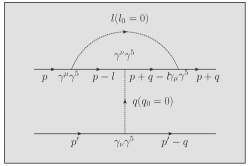
Figure 7: The Fock correction, which contributes to the wave-function renormalization constant only in the first order.
G ( 1 ) = G ( p ) ( − Γ 2 ) ∑ q γ μ γ 5 G ( p − q ) γ μ γ 5 G ( p ) G ( p ) Σ ( 1 ) G ( p ) superscript 𝐺 1 𝐺 𝑝 Γ 2 subscript 𝑞 superscript 𝛾 𝜇 superscript 𝛾 5 𝐺 𝑝 𝑞 subscript 𝛾 𝜇 superscript 𝛾 5 𝐺 𝑝 𝐺 𝑝 superscript Σ 1 𝐺 𝑝 G^{(1)}=G(p)\left(-\frac{\Gamma}{2}\right)\sum_{q}\gamma^{\mu}\gamma^{5}G(p-q)\gamma_{\mu}\gamma^{5}G(p)G(p)\Sigma^{(1)}G(p) (20)
in the one-loop order (Fig. 7 6
Omitting vacuum and one-particle reducible diagrams, we have self-energy corrections in the second order
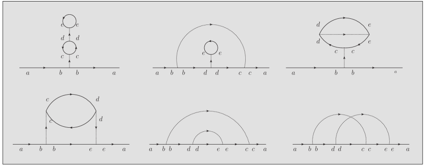
Figure 8: All possible second-order self-energy diagrams without the replica limit, omitting vacuum and one-particle reducible diagrams.
lim R → 0 1 R ∑ a , b , c , d , e [ < ψ a ψ ¯ a ψ b ¯ γ μ γ 5 ψ b ψ c ¯ γ μ γ 5 ψ c ψ d ¯ γ ν γ 5 ψ b ψ c ¯ γ ν γ 5 ψ c > 0 ] 1 P I \displaystyle\lim_{R\to 0}\frac{1}{R}\sum_{a,b,c,d,e}\biggr{[}<\psi^{a}\bar{\psi}^{a}\bar{\psi^{b}}\gamma^{\mu}\gamma^{5}\psi^{b}\bar{\psi^{c}}\gamma_{\mu}\gamma^{5}\psi^{c}\bar{\psi^{d}}\gamma^{\nu}\gamma^{5}\psi^{b}\bar{\psi^{c}}\gamma_{\nu}\gamma^{5}\psi^{c}>_{0}\biggl{]}_{1PI}
= \displaystyle= lim R → 0 1 R ∑ a , b , c , d , e [ 8 G a G b γ μ γ 5 G b G a t r [ G c γ ν γ 5 G d γ μ γ 5 ] t r [ G e γ ν γ 5 ] δ a b δ b a δ c d δ d c δ e e − 4 G a γ μ γ 5 G b γ ν γ 5 G d γ μ γ 5 \displaystyle\lim_{R\to 0}\frac{1}{R}\sum_{a,b,c,d,e}\biggr{[}8G^{a}G^{b}\gamma^{\mu}\gamma^{5}G^{b}G^{a}tr[G^{c}\gamma^{\nu}\gamma^{5}G^{d}\gamma_{\mu}\gamma^{5}]tr[G^{e}\gamma_{\nu}\gamma^{5}]\delta_{ab}\delta_{ba}\delta_{cd}\delta_{dc}\delta_{ee}-4G^{a}\gamma^{\mu}\gamma^{5}G^{b}\gamma^{\nu}\gamma^{5}G^{d}\gamma_{\mu}\gamma^{5}
× G c t r [ G e γ ν γ 5 ] δ a b δ b d δ d c δ c a δ e e − 4 G a γ μ γ 5 G b t r [ G c γ ν γ 5 G d γ ν γ 5 G e γ μ γ 5 ] δ a b δ b a δ c d δ d e δ e c + ( − 1 ) 16 G a γ μ γ 5 G b γ ν γ 5 absent superscript 𝐺 𝑐 𝑡 𝑟 delimited-[] superscript 𝐺 𝑒 subscript 𝛾 𝜈 superscript 𝛾 5 subscript 𝛿 𝑎 𝑏 subscript 𝛿 𝑏 𝑑 subscript 𝛿 𝑑 𝑐 subscript 𝛿 𝑐 𝑎 subscript 𝛿 𝑒 𝑒 4 superscript 𝐺 𝑎 superscript 𝛾 𝜇 superscript 𝛾 5 superscript 𝐺 𝑏 𝑡 𝑟 delimited-[] superscript 𝐺 𝑐 superscript 𝛾 𝜈 superscript 𝛾 5 superscript 𝐺 𝑑 subscript 𝛾 𝜈 superscript 𝛾 5 superscript 𝐺 𝑒 subscript 𝛾 𝜇 superscript 𝛾 5 subscript 𝛿 𝑎 𝑏 subscript 𝛿 𝑏 𝑎 subscript 𝛿 𝑐 𝑑 subscript 𝛿 𝑑 𝑒 subscript 𝛿 𝑒 𝑐 1 16 superscript 𝐺 𝑎 superscript 𝛾 𝜇 superscript 𝛾 5 superscript 𝐺 𝑏 subscript 𝛾 𝜈 superscript 𝛾 5 \displaystyle\times G^{c}tr[G^{e}\gamma_{\nu}\gamma^{5}]\delta_{ab}\delta_{bd}\delta_{dc}\delta_{ca}\delta_{ee}-4G^{a}\gamma^{\mu}\gamma^{5}G^{b}tr[G^{c}\gamma^{\nu}\gamma^{5}G^{d}\gamma_{\nu}\gamma^{5}G^{e}\gamma_{\mu}\gamma^{5}]\delta_{ab}\delta_{ba}\delta_{cd}\delta_{de}\delta_{ec}+(-1)16G^{a}\gamma^{\mu}\gamma^{5}G^{b}\gamma_{\nu}\gamma^{5}
× G e t r [ G c γ ν γ 5 G d γ μ γ 5 ] δ a b δ b e δ e a δ c d δ d c + 8 G a γ μ γ 5 G b γ ν γ 5 G d γ ν γ 5 G e γ μ γ 5 G c δ a b δ b d δ d e δ e c δ c a + 8 G a γ μ γ 5 G b γ ν γ 5 G d γ μ γ 5 absent superscript 𝐺 𝑒 𝑡 𝑟 delimited-[] superscript 𝐺 𝑐 superscript 𝛾 𝜈 superscript 𝛾 5 superscript 𝐺 𝑑 subscript 𝛾 𝜇 superscript 𝛾 5 subscript 𝛿 𝑎 𝑏 subscript 𝛿 𝑏 𝑒 subscript 𝛿 𝑒 𝑎 subscript 𝛿 𝑐 𝑑 subscript 𝛿 𝑑 𝑐 8 superscript 𝐺 𝑎 superscript 𝛾 𝜇 superscript 𝛾 5 superscript 𝐺 𝑏 superscript 𝛾 𝜈 superscript 𝛾 5 superscript 𝐺 𝑑 subscript 𝛾 𝜈 superscript 𝛾 5 superscript 𝐺 𝑒 subscript 𝛾 𝜇 superscript 𝛾 5 superscript 𝐺 𝑐 subscript 𝛿 𝑎 𝑏 subscript 𝛿 𝑏 𝑑 subscript 𝛿 𝑑 𝑒 subscript 𝛿 𝑒 𝑐 subscript 𝛿 𝑐 𝑎 8 superscript 𝐺 𝑎 superscript 𝛾 𝜇 superscript 𝛾 5 superscript 𝐺 𝑏 superscript 𝛾 𝜈 superscript 𝛾 5 superscript 𝐺 𝑑 subscript 𝛾 𝜇 superscript 𝛾 5 \displaystyle\times G^{e}tr[G^{c}\gamma^{\nu}\gamma^{5}G^{d}\gamma_{\mu}\gamma^{5}]\delta_{ab}\delta_{be}\delta_{ea}\delta_{cd}\delta_{dc}+8G^{a}\gamma^{\mu}\gamma^{5}G^{b}\gamma^{\nu}\gamma^{5}G^{d}\gamma_{\nu}\gamma^{5}G^{e}\gamma_{\mu}\gamma^{5}G^{c}\delta_{ab}\delta_{bd}\delta_{de}\delta_{ec}\delta_{ca}+8G^{a}\gamma^{\mu}\gamma^{5}G^{b}\gamma^{\nu}\gamma^{5}G^{d}\gamma_{\mu}\gamma^{5}
× G c γ ν γ 5 G e δ a b δ b d δ d c δ c e δ e a ] . \displaystyle\times G^{c}\gamma_{\nu}\gamma^{5}G^{e}\delta_{ab}\delta_{bd}\delta_{dc}\delta_{ce}\delta_{ea}\biggl{]}.
See Fig. 8 R 3 superscript 𝑅 3 R^{3} R 2 superscript 𝑅 2 R^{2} R 𝑅 R 9
Figure 9: Relevant second-order self-energy corrections in the replica limit.
G ( 2 ) , r ( p ) superscript 𝐺 2 𝑟
𝑝 \displaystyle G^{(2),r}(p) = \displaystyle= G ( p ) ( − Γ R 2 ) 2 ∑ q , l γ μ γ 5 G ( p − q ) γ ν γ 5 G ( p − q − l ) γ ν γ 5 G ( p − q ) γ μ γ 5 G ( p ) = G ( p ) Σ ( 2 ) , r G ( p ) 𝐺 𝑝 superscript subscript Γ 𝑅 2 2 subscript 𝑞 𝑙
superscript 𝛾 𝜇 superscript 𝛾 5 𝐺 𝑝 𝑞 superscript 𝛾 𝜈 superscript 𝛾 5 𝐺 𝑝 𝑞 𝑙 subscript 𝛾 𝜈 superscript 𝛾 5 𝐺 𝑝 𝑞 subscript 𝛾 𝜇 superscript 𝛾 5 𝐺 𝑝 𝐺 𝑝 superscript Σ 2 𝑟
𝐺 𝑝 \displaystyle G(p)\left(-\frac{\Gamma_{R}}{2}\right)^{2}\sum_{q,l}\gamma^{\mu}\gamma^{5}G(p-q)\gamma^{\nu}\gamma^{5}G(p-q-l)\gamma_{\nu}\gamma^{5}G(p-q)\gamma_{\mu}\gamma^{5}G(p)=G(p)\Sigma^{(2),r}G(p)
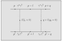
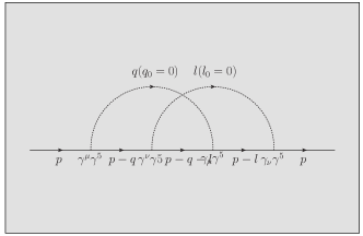
G ( 2 ) , c ( p ) superscript 𝐺 2 𝑐
𝑝 \displaystyle G^{(2),c}(p) = \displaystyle= G ( p ) ( − Γ R 2 ) 2 ∑ q , l γ μ γ 5 G ( p − q ) γ ν γ 5 G ( p − q − l ) γ μ γ 5 G ( p − l ) γ ν γ 5 G ( p ) = G ( p ) Σ ( 2 ) , c G ( p ) 𝐺 𝑝 superscript subscript Γ 𝑅 2 2 subscript 𝑞 𝑙
superscript 𝛾 𝜇 superscript 𝛾 5 𝐺 𝑝 𝑞 superscript 𝛾 𝜈 superscript 𝛾 5 𝐺 𝑝 𝑞 𝑙 subscript 𝛾 𝜇 superscript 𝛾 5 𝐺 𝑝 𝑙 subscript 𝛾 𝜈 superscript 𝛾 5 𝐺 𝑝 𝐺 𝑝 superscript Σ 2 𝑐
𝐺 𝑝 \displaystyle G(p)\left(-\frac{\Gamma_{R}}{2}\right)^{2}\sum_{q,l}\gamma^{\mu}\gamma^{5}G(p-q)\gamma^{\nu}\gamma^{5}G(p-q-l)\gamma_{\mu}\gamma^{5}G(p-l)\gamma_{\nu}\gamma^{5}G(p)=G(p)\Sigma^{(2),c}G(p)
Σ ( 2 ) , r superscript Σ 2 𝑟
\displaystyle\Sigma^{(2),r} = \displaystyle= ( − Γ R 2 ) 2 ∑ q , l γ μ γ 5 G ( p − q ) γ ν γ 5 G ( p − q − l ) γ ν γ 5 G ( p − q ) γ μ γ 5 superscript subscript Γ 𝑅 2 2 subscript 𝑞 𝑙
superscript 𝛾 𝜇 superscript 𝛾 5 𝐺 𝑝 𝑞 superscript 𝛾 𝜈 superscript 𝛾 5 𝐺 𝑝 𝑞 𝑙 subscript 𝛾 𝜈 superscript 𝛾 5 𝐺 𝑝 𝑞 subscript 𝛾 𝜇 superscript 𝛾 5 \displaystyle\left(-\frac{\Gamma_{R}}{2}\right)^{2}\sum_{q,l}\gamma^{\mu}\gamma^{5}G(p-q)\gamma^{\nu}\gamma^{5}G(p-q-l)\gamma_{\nu}\gamma^{5}G(p-q)\gamma_{\mu}\gamma^{5} (21)
Σ ( 2 ) , c superscript Σ 2 𝑐
\displaystyle\Sigma^{(2),c} = \displaystyle= ( − Γ R 2 ) 2 ∑ q , l γ μ γ 5 G ( p − q ) γ ν γ 5 G ( p − q − l ) γ μ γ 5 G ( p − l ) γ ν γ 5 . superscript subscript Γ 𝑅 2 2 subscript 𝑞 𝑙
superscript 𝛾 𝜇 superscript 𝛾 5 𝐺 𝑝 𝑞 superscript 𝛾 𝜈 superscript 𝛾 5 𝐺 𝑝 𝑞 𝑙 subscript 𝛾 𝜇 superscript 𝛾 5 𝐺 𝑝 𝑙 subscript 𝛾 𝜈 superscript 𝛾 5 \displaystyle\left(-\frac{\Gamma_{R}}{2}\right)^{2}\sum_{q,l}\gamma^{\mu}\gamma^{5}G(p-q)\gamma^{\nu}\gamma^{5}G(p-q-l)\gamma_{\mu}\gamma^{5}G(p-l)\gamma_{\nu}\gamma^{5}. (22)
D.1.2 Evaluation of relevant Feynman’s diagrams
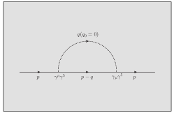
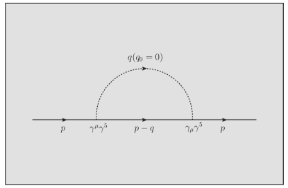
The first-order Fock diagram (Fig. 7
Σ ( 1 ) superscript Σ 1 \displaystyle\Sigma^{(1)} = \displaystyle= − Γ R 2 ∫ d d q ( 2 π ) d 2 π δ ( q 0 ) γ μ γ 5 p̸ − q̸ − m ( p − q ) 2 − m 2 γ μ γ 5 subscript Γ 𝑅 2 superscript 𝑑 𝑑 𝑞 superscript 2 𝜋 𝑑 2 𝜋 𝛿 subscript 𝑞 0 superscript 𝛾 𝜇 superscript 𝛾 5 italic-p̸ italic-q̸ 𝑚 superscript 𝑝 𝑞 2 superscript 𝑚 2 superscript 𝛾 𝜇 superscript 𝛾 5 \displaystyle-\frac{\Gamma_{R}}{2}\int\frac{d^{d}q}{(2\pi)^{d}}2\pi\delta(q_{0})\gamma^{\mu}\gamma^{5}\frac{\not{p}-\not{q}-m}{(p-q)^{2}-m^{2}}\gamma^{\mu}\gamma^{5}
= \displaystyle= − Γ R 2 ∫ d d − 1 𝒒 ( 2 π ) d − 1 γ μ ( p 0 γ 0 + p k γ k − q k γ k + m ) γ μ − p 0 2 − ( 𝒑 − 𝒒 ) 2 − m 2 subscript Γ 𝑅 2 superscript 𝑑 𝑑 1 𝒒 superscript 2 𝜋 𝑑 1 superscript 𝛾 𝜇 subscript 𝑝 0 superscript 𝛾 0 subscript 𝑝 𝑘 superscript 𝛾 𝑘 subscript 𝑞 𝑘 superscript 𝛾 𝑘 𝑚 subscript 𝛾 𝜇 superscript subscript 𝑝 0 2 superscript 𝒑 𝒒 2 superscript 𝑚 2 \displaystyle-\frac{\Gamma_{R}}{2}\int\frac{d^{d-1}\bm{q}}{(2\pi)^{d-1}}\frac{\gamma^{\mu}(p_{0}\gamma^{0}+p_{k}\gamma^{k}-q_{k}\gamma^{k}+m)\gamma_{\mu}}{-p_{0}^{2}-(\bm{p}-\bm{q})^{2}-m^{2}}
= \displaystyle= Γ R 2 ∫ d d − 1 𝒒 ( 2 π ) d − 1 ( 2 − d ) q k γ k − 2 p 0 γ 0 + 4 m 𝒒 2 + p 0 2 + m 2 subscript Γ 𝑅 2 superscript 𝑑 𝑑 1 𝒒 superscript 2 𝜋 𝑑 1 2 𝑑 subscript 𝑞 𝑘 superscript 𝛾 𝑘 2 subscript 𝑝 0 superscript 𝛾 0 4 𝑚 superscript 𝒒 2 superscript subscript 𝑝 0 2 superscript 𝑚 2 \displaystyle\frac{\Gamma_{R}}{2}\int\frac{d^{d-1}\bm{q}}{(2\pi)^{d-1}}\frac{(2-d)q_{k}\gamma^{k}-2p_{0}\gamma^{0}+4m}{\bm{q}^{2}+p_{0}^{2}+m^{2}}
= \displaystyle= Γ R 2 [ − 2 p 0 γ 0 + 4 m ( 4 π ) d − 1 2 Γ ( 1 − d − 1 2 ) Γ ( 1 ) 1 ( p 0 2 + m 2 ) 1 = d − 1 2 ] subscript Γ 𝑅 2 delimited-[] 2 subscript 𝑝 0 superscript 𝛾 0 4 𝑚 superscript 4 𝜋 𝑑 1 2 Γ 1 𝑑 1 2 Γ 1 1 superscript superscript subscript 𝑝 0 2 superscript 𝑚 2 1 𝑑 1 2 \displaystyle\frac{\Gamma_{R}}{2}\left[\frac{-2p_{0}\gamma^{0}+4m}{(4\pi)^{\frac{d-1}{2}}}\frac{\Gamma(1-\frac{d-1}{2})}{\Gamma(1)}\frac{1}{(p_{0}^{2}+m^{2})^{1=\frac{d-1}{2}}}\right]
= \displaystyle= Γ R 2 ( 4 π ) ( − 2 p 0 γ 0 + 4 m ) ( − 2 ϵ − γ − log ( p 0 2 + m 2 ) + log 4 π + O ( ϵ ) ) . \displaystyle\frac{\Gamma_{R}}{2(4\pi)}(-2p_{0}\gamma^{0}+4m)\biggr{(}-\frac{2}{\epsilon}-\gamma-\log{(p_{0}^{2}+m^{2})}+\log{4\pi}+O(\epsilon)\biggl{)}.
Then, a relevant part for renormalization is
Σ ( 1 ) = − Γ R 4 π 1 ϵ ( − 2 p 0 γ 0 + 4 m ) + O ( 1 ) superscript Σ 1 subscript Γ 𝑅 4 𝜋 1 italic-ϵ 2 subscript 𝑝 0 superscript 𝛾 0 4 𝑚 𝑂 1 \Sigma^{(1)}=-\frac{\Gamma_{R}}{4\pi}\frac{1}{\epsilon}(-2p_{0}\gamma^{0}+4m)+O(1) (23)
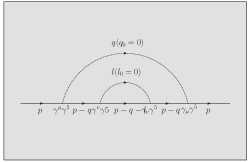
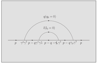
The second-order rainbow diagram (the first diagram in Fig. 9
Σ ( 2 ) , r superscript Σ 2 𝑟
\displaystyle\Sigma^{(2),r} = \displaystyle= ( − Γ R 2 ) 2 ∫ d d q ( 2 π ) d 2 π δ ( q 0 ) ∫ d d l ( 2 π ) d 2 π δ ( l 0 ) γ μ γ 5 p̸ − q̸ − m ( p − q ) 2 − m 2 γ ν γ 5 p̸ − q̸ − l̸ − m ( p − q − l ) 2 − m 2 γ ν γ 5 superscript subscript Γ 𝑅 2 2 superscript 𝑑 𝑑 𝑞 superscript 2 𝜋 𝑑 2 𝜋 𝛿 subscript 𝑞 0 superscript 𝑑 𝑑 𝑙 superscript 2 𝜋 𝑑 2 𝜋 𝛿 subscript 𝑙 0 superscript 𝛾 𝜇 superscript 𝛾 5 italic-p̸ italic-q̸ 𝑚 superscript 𝑝 𝑞 2 superscript 𝑚 2 superscript 𝛾 𝜈 superscript 𝛾 5 italic-p̸ italic-q̸ italic-l̸ 𝑚 superscript 𝑝 𝑞 𝑙 2 superscript 𝑚 2 subscript 𝛾 𝜈 superscript 𝛾 5 \displaystyle\left(-\frac{\Gamma_{R}}{2}\right)^{2}\int\frac{d^{d}q}{(2\pi)^{d}}2\pi\delta(q_{0})\int\frac{d^{d}l}{(2\pi)^{d}}2\pi\delta(l_{0})\gamma^{\mu}\gamma^{5}\frac{\not{p}-\not{q}-m}{(p-q)^{2}-m^{2}}\gamma^{\nu}\gamma^{5}\frac{\not{p}-\not{q}-\not{l}-m}{(p-q-l)^{2}-m^{2}}\gamma_{\nu}\gamma^{5}
× p̸ − q̸ − m ( p − q ) 2 − m 2 γ μ γ 5 absent italic-p̸ italic-q̸ 𝑚 superscript 𝑝 𝑞 2 superscript 𝑚 2 subscript 𝛾 𝜇 superscript 𝛾 5 \displaystyle\times\frac{\not{p}-\not{q}-m}{(p-q)^{2}-m^{2}}\gamma_{\mu}\gamma^{5}
= \displaystyle= Γ R 2 4 ∫ d d − 1 𝒒 ( 2 π ) d − 1 ∫ d d − 1 𝒍 ( 2 π ) d − 1 γ μ p 0 γ 0 + p k γ k − q k γ k + m − p 0 2 − ( 𝒑 − 𝒒 ) 2 − m 2 γ ν p 0 γ 0 + p l γ l − q l γ l − l l γ l − m − p 0 2 − ( 𝒑 − 𝒒 − 𝒍 ) 2 − m 2 γ ν superscript subscript Γ 𝑅 2 4 superscript 𝑑 𝑑 1 𝒒 superscript 2 𝜋 𝑑 1 superscript 𝑑 𝑑 1 𝒍 superscript 2 𝜋 𝑑 1 superscript 𝛾 𝜇 subscript 𝑝 0 superscript 𝛾 0 subscript 𝑝 𝑘 superscript 𝛾 𝑘 subscript 𝑞 𝑘 superscript 𝛾 𝑘 𝑚 superscript subscript 𝑝 0 2 superscript 𝒑 𝒒 2 superscript 𝑚 2 superscript 𝛾 𝜈 subscript 𝑝 0 superscript 𝛾 0 subscript 𝑝 𝑙 superscript 𝛾 𝑙 subscript 𝑞 𝑙 superscript 𝛾 𝑙 subscript 𝑙 𝑙 superscript 𝛾 𝑙 𝑚 superscript subscript 𝑝 0 2 superscript 𝒑 𝒒 𝒍 2 superscript 𝑚 2 subscript 𝛾 𝜈 \displaystyle\frac{\Gamma_{R}^{2}}{4}\int\frac{d^{d-1}\bm{q}}{(2\pi)^{d-1}}\int\frac{d^{d-1}\bm{l}}{(2\pi)^{d-1}}\gamma^{\mu}\frac{p_{0}\gamma^{0}+p_{k}\gamma^{k}-q_{k}\gamma^{k}+m}{-p_{0}^{2}-(\bm{p}-\bm{q})^{2}-m^{2}}\gamma^{\nu}\frac{p_{0}\gamma^{0}+p_{l}\gamma^{l}-q_{l}\gamma^{l}-l_{l}\gamma^{l}-m}{-p_{0}^{2}-(\bm{p}-\bm{q}-\bm{l})^{2}-m^{2}}\gamma_{\nu}
× p 0 γ 0 + p m γ m − q m γ m + m − p 0 2 − ( 𝒑 − 𝒒 ) 2 − m 2 γ μ absent subscript 𝑝 0 superscript 𝛾 0 subscript 𝑝 𝑚 superscript 𝛾 𝑚 subscript 𝑞 𝑚 superscript 𝛾 𝑚 𝑚 superscript subscript 𝑝 0 2 superscript 𝒑 𝒒 2 superscript 𝑚 2 subscript 𝛾 𝜇 \displaystyle\times\frac{p_{0}\gamma^{0}+p_{m}\gamma^{m}-q_{m}\gamma^{m}+m}{-p_{0}^{2}-(\bm{p}-\bm{q})^{2}-m^{2}}\gamma_{\mu}
= \displaystyle= − Γ R 2 4 ∫ d d − 1 𝒒 ( 2 π ) d − 1 γ μ p 0 γ 0 + p k γ k − q k γ k + m ( 𝒑 − 𝒒 ) 2 + p 0 2 + m 2 γ ν [ ∫ d d − 1 𝒍 ( 2 π ) d − 1 p 0 γ 0 + p l γ l − q l γ l − l l γ l − m ( 𝒑 − 𝒒 − 𝒍 ) 2 + p 0 2 + m 2 ] γ ν \displaystyle-\frac{\Gamma_{R}^{2}}{4}\int\frac{d^{d-1}\bm{q}}{(2\pi)^{d-1}}\gamma^{\mu}\frac{p_{0}\gamma^{0}+p_{k}\gamma^{k}-q_{k}\gamma^{k}+m}{(\bm{p}-\bm{q})^{2}+p_{0}^{2}+m^{2}}\gamma^{\nu}\biggr{[}\int\frac{d^{d-1}\bm{l}}{(2\pi)^{d-1}}\frac{p_{0}\gamma^{0}+p_{l}\gamma^{l}-q_{l}\gamma^{l}-l_{l}\gamma^{l}-m}{(\bm{p}-\bm{q}-\bm{l})^{2}+p_{0}^{2}+m^{2}}\biggl{]}\gamma_{\nu}
× p 0 γ 0 + p m γ m − q m γ m + m ( 𝒑 − 𝒒 ) 2 + p 0 2 + m 2 γ μ absent subscript 𝑝 0 superscript 𝛾 0 subscript 𝑝 𝑚 superscript 𝛾 𝑚 subscript 𝑞 𝑚 superscript 𝛾 𝑚 𝑚 superscript 𝒑 𝒒 2 superscript subscript 𝑝 0 2 superscript 𝑚 2 subscript 𝛾 𝜇 \displaystyle\times\frac{p_{0}\gamma^{0}+p_{m}\gamma^{m}-q_{m}\gamma^{m}+m}{(\bm{p}-\bm{q})^{2}+p_{0}^{2}+m^{2}}\gamma_{\mu}
= \displaystyle= − Γ R 2 4 ∫ d d − 1 𝒒 ( 2 π ) d − 1 γ μ − q k γ k + p 0 γ 0 + m 𝒒 2 + p 0 2 + m 2 γ ν [ ∫ d d − 1 𝒍 ( 2 π ) d − 1 − l l γ l + p 0 γ 0 − m 𝒍 2 + p 0 2 + m 2 ] γ ν − q m γ m + p 0 γ 0 + m 𝒒 2 + p 0 2 + m 2 γ μ \displaystyle-\frac{\Gamma_{R}^{2}}{4}\int\frac{d^{d-1}\bm{q}}{(2\pi)^{d-1}}\gamma^{\mu}\frac{-q_{k}\gamma^{k}+p_{0}\gamma^{0}+m}{\bm{q}^{2}+p_{0}^{2}+m^{2}}\gamma^{\nu}\biggr{[}\int\frac{d^{d-1}\bm{l}}{(2\pi)^{d-1}}\frac{-l_{l}\gamma^{l}+p_{0}\gamma^{0}-m}{\bm{l}^{2}+p_{0}^{2}+m^{2}}\biggl{]}\gamma_{\nu}\frac{-q_{m}\gamma^{m}+p_{0}\gamma^{0}+m}{\bm{q}^{2}+p_{0}^{2}+m^{2}}\gamma_{\mu}
= \displaystyle= − Γ R 2 4 ∫ d d − 1 𝒒 ( 2 π ) d − 1 γ μ − q k γ k + p 0 γ 0 + m 𝒒 2 + p 0 2 + m 2 [ 1 ( 4 π ) d − 1 2 Γ ( 1 − d − 1 2 ) Γ ( 1 ) γ ν ( p 0 γ 0 − m ) γ ν ( p 0 2 + m 2 ) 1 − d − 1 2 ] − q m γ m + p 0 γ 0 + m 𝒒 2 + p 0 2 + m 2 γ μ \displaystyle-\frac{\Gamma_{R}^{2}}{4}\int\frac{d^{d-1}\bm{q}}{(2\pi)^{d-1}}\gamma^{\mu}\frac{-q_{k}\gamma^{k}+p_{0}\gamma^{0}+m}{\bm{q}^{2}+p_{0}^{2}+m^{2}}\biggr{[}\frac{1}{(4\pi)^{\frac{d-1}{2}}}\frac{\Gamma(1-\frac{d-1}{2})}{\Gamma(1)}\frac{\gamma^{\nu}(p_{0}\gamma^{0}-m)\gamma_{\nu}}{(p_{0}^{2}+m^{2})^{1-\frac{d-1}{2}}}\biggl{]}\frac{-q_{m}\gamma^{m}+p_{0}\gamma^{0}+m}{\bm{q}^{2}+p_{0}^{2}+m^{2}}\gamma_{\mu}
= \displaystyle= − Γ R 2 4 Γ ( 3 − d 2 ) ( 4 π ) d − 1 2 ( p 0 2 + m 2 ) 3 − d 2 ∫ d d − 1 𝒒 ( 2 π ) d − 1 γ μ ( − q k γ k + p 0 γ 0 + m ) ( − 2 p 0 γ 0 − 4 m ) ( − q m γ m + p 0 γ 0 + m ) γ μ ( 𝒒 2 + p 0 2 + m 2 ) 2 . superscript subscript Γ 𝑅 2 4 Γ 3 𝑑 2 superscript 4 𝜋 𝑑 1 2 superscript superscript subscript 𝑝 0 2 superscript 𝑚 2 3 𝑑 2 superscript 𝑑 𝑑 1 𝒒 superscript 2 𝜋 𝑑 1 superscript 𝛾 𝜇 subscript 𝑞 𝑘 superscript 𝛾 𝑘 subscript 𝑝 0 superscript 𝛾 0 𝑚 2 subscript 𝑝 0 superscript 𝛾 0 4 𝑚 subscript 𝑞 𝑚 superscript 𝛾 𝑚 subscript 𝑝 0 superscript 𝛾 0 𝑚 subscript 𝛾 𝜇 superscript superscript 𝒒 2 superscript subscript 𝑝 0 2 superscript 𝑚 2 2 \displaystyle-\frac{\Gamma_{R}^{2}}{4}\frac{\Gamma(\frac{3-d}{2})}{(4\pi)^{\frac{d-1}{2}}(p_{0}^{2}+m^{2})^{\frac{3-d}{2}}}\int\frac{d^{d-1}\bm{q}}{(2\pi)^{d-1}}\frac{\gamma^{\mu}(-q_{k}\gamma^{k}+p_{0}\gamma^{0}+m)(-2p_{0}\gamma^{0}-4m)(-q_{m}\gamma^{m}+p_{0}\gamma^{0}+m)\gamma_{\mu}}{(\bm{q}^{2}+p_{0}^{2}+m^{2})^{2}}.
Rearranging the numerator as follows
N 𝑁 \displaystyle N = \displaystyle= γ μ ( − q k γ k + p 0 γ 0 + m ) ( − 2 p 0 γ 0 − 4 m ) ( − q m γ m + p 0 γ 0 + m ) γ μ superscript 𝛾 𝜇 subscript 𝑞 𝑘 superscript 𝛾 𝑘 subscript 𝑝 0 superscript 𝛾 0 𝑚 2 subscript 𝑝 0 superscript 𝛾 0 4 𝑚 subscript 𝑞 𝑚 superscript 𝛾 𝑚 subscript 𝑝 0 superscript 𝛾 0 𝑚 subscript 𝛾 𝜇 \displaystyle\gamma^{\mu}(-q_{k}\gamma^{k}+p_{0}\gamma^{0}+m)(-2p_{0}\gamma^{0}-4m)(-q_{m}\gamma^{m}+p_{0}\gamma^{0}+m)\gamma_{\mu}
= \displaystyle= − q k q m γ μ γ k ( 2 p 0 γ 0 + 4 m ) γ m γ μ − γ μ ( p 0 γ 0 + m ) ( 2 p 0 γ 0 + 4 m ) ( p 0 γ 0 + m ) γ μ subscript 𝑞 𝑘 subscript 𝑞 𝑚 superscript 𝛾 𝜇 superscript 𝛾 𝑘 2 subscript 𝑝 0 superscript 𝛾 0 4 𝑚 superscript 𝛾 𝑚 subscript 𝛾 𝜇 superscript 𝛾 𝜇 subscript 𝑝 0 superscript 𝛾 0 𝑚 2 subscript 𝑝 0 superscript 𝛾 0 4 𝑚 subscript 𝑝 0 superscript 𝛾 0 𝑚 subscript 𝛾 𝜇 \displaystyle-q_{k}q_{m}\gamma^{\mu}\gamma^{k}(2p_{0}\gamma^{0}+4m)\gamma^{m}\gamma_{\mu}-\gamma^{\mu}(p_{0}\gamma^{0}+m)(2p_{0}\gamma^{0}+4m)(p_{0}\gamma^{0}+m)\gamma_{\mu}
= \displaystyle= − q k q m γ μ γ k ( 2 p 0 γ 0 + 4 m ) γ m γ μ + ( − 4 p 0 3 γ 0 + 32 m p 0 2 + 20 m 2 p 0 γ 0 − 16 m 3 ) subscript 𝑞 𝑘 subscript 𝑞 𝑚 superscript 𝛾 𝜇 superscript 𝛾 𝑘 2 subscript 𝑝 0 superscript 𝛾 0 4 𝑚 superscript 𝛾 𝑚 subscript 𝛾 𝜇 4 superscript subscript 𝑝 0 3 superscript 𝛾 0 32 𝑚 superscript subscript 𝑝 0 2 20 superscript 𝑚 2 subscript 𝑝 0 superscript 𝛾 0 16 superscript 𝑚 3 \displaystyle-q_{k}q_{m}\gamma^{\mu}\gamma^{k}(2p_{0}\gamma^{0}+4m)\gamma^{m}\gamma_{\mu}+(-4p_{0}^{3}\gamma^{0}+32mp_{0}^{2}+20m^{2}p_{0}\gamma^{0}-16m^{3})
= \displaystyle= − q k q m γ μ γ k ( 2 p 0 γ 0 + 4 m ) γ m γ μ + f ( p ) subscript 𝑞 𝑘 subscript 𝑞 𝑚 superscript 𝛾 𝜇 superscript 𝛾 𝑘 2 subscript 𝑝 0 superscript 𝛾 0 4 𝑚 superscript 𝛾 𝑚 subscript 𝛾 𝜇 𝑓 𝑝 \displaystyle-q_{k}q_{m}\gamma^{\mu}\gamma^{k}(2p_{0}\gamma^{0}+4m)\gamma^{m}\gamma_{\mu}+f(p)
with f ( p ) = − 4 p 0 3 γ 0 + 32 m p 0 2 + 20 m 2 p 0 γ 0 − 16 m 3 𝑓 𝑝 4 superscript subscript 𝑝 0 3 superscript 𝛾 0 32 𝑚 superscript subscript 𝑝 0 2 20 superscript 𝑚 2 subscript 𝑝 0 superscript 𝛾 0 16 superscript 𝑚 3 f(p)=-4p_{0}^{3}\gamma^{0}+32mp_{0}^{2}+20m^{2}p_{0}\gamma^{0}-16m^{3}
Σ ( 2 ) , r superscript Σ 2 𝑟
\displaystyle\Sigma^{(2),r} = \displaystyle= − Γ R 2 4 Γ ( 3 − d 2 ) ( 4 π ) d − 1 2 ( p 0 2 + m 2 ) 3 − d 2 ∫ d d − 1 𝒒 ( 2 π ) d − 1 − q k q m γ μ γ k ( 2 p 0 γ 0 + 4 m ) γ m γ μ + f ( p ) ( 𝒒 2 + p 0 2 + m 2 ) 2 superscript subscript Γ 𝑅 2 4 Γ 3 𝑑 2 superscript 4 𝜋 𝑑 1 2 superscript superscript subscript 𝑝 0 2 superscript 𝑚 2 3 𝑑 2 superscript 𝑑 𝑑 1 𝒒 superscript 2 𝜋 𝑑 1 subscript 𝑞 𝑘 subscript 𝑞 𝑚 superscript 𝛾 𝜇 superscript 𝛾 𝑘 2 subscript 𝑝 0 superscript 𝛾 0 4 𝑚 superscript 𝛾 𝑚 subscript 𝛾 𝜇 𝑓 𝑝 superscript superscript 𝒒 2 superscript subscript 𝑝 0 2 superscript 𝑚 2 2 \displaystyle-\frac{\Gamma_{R}^{2}}{4}\frac{\Gamma(\frac{3-d}{2})}{(4\pi)^{\frac{d-1}{2}}(p_{0}^{2}+m^{2})^{\frac{3-d}{2}}}\int\frac{d^{d-1}\bm{q}}{(2\pi)^{d-1}}\frac{-q_{k}q_{m}\gamma^{\mu}\gamma^{k}(2p_{0}\gamma^{0}+4m)\gamma^{m}\gamma_{\mu}+f(p)}{(\bm{q}^{2}+p_{0}^{2}+m^{2})^{2}}
= \displaystyle= − Γ R 2 4 Γ ( 3 − d 2 ) ( 4 π ) d − 1 2 ( p 0 2 + m 2 ) 3 − d 2 [ − γ μ γ k ( 2 p 0 γ 0 + 4 m ) γ k γ μ 2 ( 4 π ) d − 1 2 Γ ( 2 − d − 1 2 − 1 ) Γ ( 2 ) ( p 0 2 + m 2 ) 2 − d − 1 2 − 1 + f ( p ) ( 4 π ) d − 1 2 Γ ( 2 − d − 1 2 ) Γ ( 2 ) ( p 0 2 + m 2 ) 2 − d − 1 2 ] \displaystyle-\frac{\Gamma_{R}^{2}}{4}\frac{\Gamma(\frac{3-d}{2})}{(4\pi)^{\frac{d-1}{2}}(p_{0}^{2}+m^{2})^{\frac{3-d}{2}}}\biggr{[}-\frac{\gamma^{\mu}\gamma^{k}(2p_{0}\gamma^{0}+4m)\gamma_{k}\gamma_{\mu}}{2(4\pi)^{\frac{d-1}{2}}}\frac{\Gamma(2-\frac{d-1}{2}-1)}{\Gamma(2)(p_{0}^{2}+m^{2})^{2-\frac{d-1}{2}-1}}+\frac{f(p)}{(4\pi)^{\frac{d-1}{2}}}\frac{\Gamma(2-\frac{d-1}{2})}{\Gamma(2)(p_{0}^{2}+m^{2})^{2-\frac{d-1}{2}}}\biggl{]}
= \displaystyle= − Γ R 2 4 Γ ( 3 − d 2 ) ( 4 π ) d − 1 2 ( p 0 2 + m 2 ) 3 − d 2 [ − 2 ( d − 2 ) ( d − 1 ) p 0 γ 0 + 4 d ( d − 1 ) m 2 ( 4 π ) d − 1 2 Γ ( 3 − d 2 ) ( p 0 2 + m 2 ) 3 − d 2 + f ( p ) ( 4 π ) d − 1 2 Γ ( 5 − d 2 ) ( p 0 2 + m 2 ) 5 − d 2 ] \displaystyle-\frac{\Gamma_{R}^{2}}{4}\frac{\Gamma(\frac{3-d}{2})}{(4\pi)^{\frac{d-1}{2}}(p_{0}^{2}+m^{2})^{\frac{3-d}{2}}}\biggr{[}-\frac{2(d-2)(d-1)p_{0}\gamma^{0}+4d(d-1)m}{2(4\pi)^{\frac{d-1}{2}}}\frac{\Gamma(\frac{3-d}{2})}{(p_{0}^{2}+m^{2})^{\frac{3-d}{2}}}+\frac{f(p)}{(4\pi)^{\frac{d-1}{2}}}\frac{\Gamma(\frac{5-d}{2})}{(p_{0}^{2}+m^{2})^{\frac{5-d}{2}}}\biggl{]}
= \displaystyle= Γ R 2 4 ( 4 π ) 2 ( − 2 ϵ − γ + log ( 4 π ) − log ( p 0 2 + m 2 ) + O ( ϵ ) ) 2 ( ( 1 + ϵ ) ( 2 + ϵ ) p 0 γ 0 + 2 ( 3 + ϵ ) ( 2 + ϵ ) m ) superscript subscript Γ 𝑅 2 4 superscript 4 𝜋 2 superscript 2 italic-ϵ 𝛾 4 𝜋 superscript subscript 𝑝 0 2 superscript 𝑚 2 𝑂 italic-ϵ 2 1 italic-ϵ 2 italic-ϵ subscript 𝑝 0 superscript 𝛾 0 2 3 italic-ϵ 2 italic-ϵ 𝑚 \displaystyle\frac{\Gamma_{R}^{2}}{4(4\pi)^{2}}\left(-\frac{2}{\epsilon}-\gamma+\log{(4\pi)}-\log{(p_{0}^{2}+m^{2})}+O(\epsilon)\right)^{2}\left((1+\epsilon)(2+\epsilon)p_{0}\gamma^{0}+2(3+\epsilon)(2+\epsilon)m\right)
− Γ 2 4 ( 4 π ) 2 ( − 2 ϵ − γ + log ( 4 π ) − log ( p 0 2 + m 2 ) + O ( ϵ ) ) 2 ( − ϵ 2 ) − 4 p 0 3 γ 0 + 32 m p 0 2 + 20 m 2 p 0 γ 0 − 16 m 3 p 0 2 + m 2 . superscript Γ 2 4 superscript 4 𝜋 2 superscript 2 italic-ϵ 𝛾 4 𝜋 superscript subscript 𝑝 0 2 superscript 𝑚 2 𝑂 italic-ϵ 2 italic-ϵ 2 4 superscript subscript 𝑝 0 3 superscript 𝛾 0 32 𝑚 superscript subscript 𝑝 0 2 20 superscript 𝑚 2 subscript 𝑝 0 superscript 𝛾 0 16 superscript 𝑚 3 superscript subscript 𝑝 0 2 superscript 𝑚 2 \displaystyle-\frac{\Gamma^{2}}{4(4\pi)^{2}}\left(-\frac{2}{\epsilon}-\gamma+\log{(4\pi)}-\log{(p_{0}^{2}+m^{2})}+O(\epsilon)\right)^{2}\left(-\frac{\epsilon}{2}\right)\frac{-4p_{0}^{3}\gamma^{0}+32mp_{0}^{2}+20m^{2}p_{0}\gamma^{0}-16m^{3}}{p_{0}^{2}+m^{2}}.
We note that the second term vanishes when we use the on-shell condition, given by p 0 γ 0 + m = 0 subscript 𝑝 0 superscript 𝛾 0 𝑚 0 p_{0}\gamma^{0}+m=0 p 0 2 = m 2 superscript subscript 𝑝 0 2 superscript 𝑚 2 p_{0}^{2}=m^{2}
Σ ( 2 ) , r = Γ R 2 16 π 2 1 ϵ ( 3 p 0 γ 0 + 10 m ) + O ( 1 ) + O ( ϵ − 2 ) . superscript Σ 2 𝑟
superscript subscript Γ 𝑅 2 16 superscript 𝜋 2 1 italic-ϵ 3 subscript 𝑝 0 superscript 𝛾 0 10 𝑚 𝑂 1 𝑂 superscript italic-ϵ 2 \Sigma^{(2),r}=\frac{\Gamma_{R}^{2}}{16\pi^{2}}\frac{1}{\epsilon}(3p_{0}\gamma^{0}+10m)+O(1)+O\left(\epsilon^{-2}\right). (24)
The second-order crossed diagram (the second diagram in Fig. 9
Σ ( 2 ) , c superscript Σ 2 𝑐
\displaystyle\Sigma^{(2),c} = \displaystyle= ( − Γ R 2 ) 2 ∫ d d q ( 2 π ) d 2 π δ ( q 0 ) ∫ d d l ( 2 π ) d 2 π δ ( l 0 ) γ μ γ 5 p̸ − q̸ − m ( p − q ) 2 − m 2 γ ν γ 5 p̸ − q̸ − l̸ − m ( p − q − l ) 2 − m 2 γ μ γ 5 p̸ − l̸ − m ( p − l ) 2 − m 2 γ ν γ 5 superscript subscript Γ 𝑅 2 2 superscript 𝑑 𝑑 𝑞 superscript 2 𝜋 𝑑 2 𝜋 𝛿 subscript 𝑞 0 superscript 𝑑 𝑑 𝑙 superscript 2 𝜋 𝑑 2 𝜋 𝛿 subscript 𝑙 0 superscript 𝛾 𝜇 superscript 𝛾 5 italic-p̸ italic-q̸ 𝑚 superscript 𝑝 𝑞 2 superscript 𝑚 2 superscript 𝛾 𝜈 superscript 𝛾 5 italic-p̸ italic-q̸ italic-l̸ 𝑚 superscript 𝑝 𝑞 𝑙 2 superscript 𝑚 2 subscript 𝛾 𝜇 superscript 𝛾 5 italic-p̸ italic-l̸ 𝑚 superscript 𝑝 𝑙 2 superscript 𝑚 2 superscript 𝛾 𝜈 superscript 𝛾 5 \displaystyle\left(-\frac{\Gamma_{R}}{2}\right)^{2}\int\frac{d^{d}q}{(2\pi)^{d}}2\pi\delta(q_{0})\int\frac{d^{d}l}{(2\pi)^{d}}2\pi\delta(l_{0})\gamma^{\mu}\gamma^{5}\frac{\not{p}-\not{q}-m}{(p-q)^{2}-m^{2}}\gamma^{\nu}\gamma^{5}\frac{\not{p}-\not{q}-\not{l}-m}{(p-q-l)^{2}-m^{2}}\gamma_{\mu}\gamma^{5}\frac{\not{p}-\not{l}-m}{(p-l)^{2}-m^{2}}\gamma^{\nu}\gamma^{5}
= \displaystyle= Γ R 2 4 ∫ d d − 1 𝒒 ( 2 π ) d − 1 ∫ d d − 1 𝒍 ( 2 π ) d − 1 γ μ p 0 γ 0 + p k γ k − q k γ k + m − p 0 2 − ( 𝒑 − 𝒒 ) 2 − m 2 γ ν p 0 γ 0 + p l γ l − q l γ l − l l γ l − m − p 0 2 − ( 𝒑 − 𝒒 − 𝒍 ) 2 − m 2 γ μ superscript subscript Γ 𝑅 2 4 superscript 𝑑 𝑑 1 𝒒 superscript 2 𝜋 𝑑 1 superscript 𝑑 𝑑 1 𝒍 superscript 2 𝜋 𝑑 1 superscript 𝛾 𝜇 subscript 𝑝 0 superscript 𝛾 0 subscript 𝑝 𝑘 superscript 𝛾 𝑘 subscript 𝑞 𝑘 superscript 𝛾 𝑘 𝑚 superscript subscript 𝑝 0 2 superscript 𝒑 𝒒 2 superscript 𝑚 2 superscript 𝛾 𝜈 subscript 𝑝 0 superscript 𝛾 0 subscript 𝑝 𝑙 superscript 𝛾 𝑙 subscript 𝑞 𝑙 superscript 𝛾 𝑙 subscript 𝑙 𝑙 superscript 𝛾 𝑙 𝑚 superscript subscript 𝑝 0 2 superscript 𝒑 𝒒 𝒍 2 superscript 𝑚 2 subscript 𝛾 𝜇 \displaystyle\frac{\Gamma_{R}^{2}}{4}\int\frac{d^{d-1}\bm{q}}{(2\pi)^{d-1}}\int\frac{d^{d-1}\bm{l}}{(2\pi)^{d-1}}\gamma^{\mu}\frac{p_{0}\gamma^{0}+p_{k}\gamma^{k}-q_{k}\gamma^{k}+m}{-p_{0}^{2}-(\bm{p}-\bm{q})^{2}-m^{2}}\gamma^{\nu}\frac{p_{0}\gamma^{0}+p_{l}\gamma^{l}-q_{l}\gamma^{l}-l_{l}\gamma^{l}-m}{-p_{0}^{2}-(\bm{p}-\bm{q}-\bm{l})^{2}-m^{2}}\gamma_{\mu}
× p 0 γ 0 + p m γ m − l m γ m + m − p 0 2 − ( 𝒑 − 𝒍 ) 2 − m 2 γ ν absent subscript 𝑝 0 superscript 𝛾 0 subscript 𝑝 𝑚 superscript 𝛾 𝑚 subscript 𝑙 𝑚 superscript 𝛾 𝑚 𝑚 superscript subscript 𝑝 0 2 superscript 𝒑 𝒍 2 superscript 𝑚 2 subscript 𝛾 𝜈 \displaystyle\times\frac{p_{0}\gamma^{0}+p_{m}\gamma^{m}-l_{m}\gamma^{m}+m}{-p_{0}^{2}-(\bm{p}-\bm{l})^{2}-m^{2}}\gamma_{\nu}
= \displaystyle= − Γ R 2 4 ∫ d d − 1 𝒍 ( 2 π ) d − 1 ∫ d d − 1 𝒒 ( 2 π ) d − 1 γ μ − q k γ k + p 0 γ 0 + m 𝒒 2 + p 0 2 + m 2 γ ν − q l γ l − l l γ l − p l γ l + p 0 γ 0 − m ( 𝒒 + 𝒍 + 𝒑 ) 2 + p 0 2 + m 2 γ μ − l m γ m + p 0 γ 0 + m 𝒍 2 + p 0 2 + m 2 γ ν superscript subscript Γ 𝑅 2 4 superscript 𝑑 𝑑 1 𝒍 superscript 2 𝜋 𝑑 1 superscript 𝑑 𝑑 1 𝒒 superscript 2 𝜋 𝑑 1 superscript 𝛾 𝜇 subscript 𝑞 𝑘 superscript 𝛾 𝑘 subscript 𝑝 0 superscript 𝛾 0 𝑚 superscript 𝒒 2 superscript subscript 𝑝 0 2 superscript 𝑚 2 superscript 𝛾 𝜈 subscript 𝑞 𝑙 superscript 𝛾 𝑙 subscript 𝑙 𝑙 superscript 𝛾 𝑙 subscript 𝑝 𝑙 superscript 𝛾 𝑙 subscript 𝑝 0 superscript 𝛾 0 𝑚 superscript 𝒒 𝒍 𝒑 2 superscript subscript 𝑝 0 2 superscript 𝑚 2 subscript 𝛾 𝜇 subscript 𝑙 𝑚 superscript 𝛾 𝑚 subscript 𝑝 0 superscript 𝛾 0 𝑚 superscript 𝒍 2 superscript subscript 𝑝 0 2 superscript 𝑚 2 subscript 𝛾 𝜈 \displaystyle-\frac{\Gamma_{R}^{2}}{4}\int\frac{d^{d-1}\bm{l}}{(2\pi)^{d-1}}\int\frac{d^{d-1}\bm{q}}{(2\pi)^{d-1}}\gamma^{\mu}\frac{-q_{k}\gamma^{k}+p_{0}\gamma^{0}+m}{\bm{q}^{2}+p_{0}^{2}+m^{2}}\gamma^{\nu}\frac{-q_{l}\gamma^{l}-l_{l}\gamma^{l}-p_{l}\gamma^{l}+p_{0}\gamma^{0}-m}{(\bm{q}+\bm{l}+\bm{p})^{2}+p_{0}^{2}+m^{2}}\gamma_{\mu}\frac{-l_{m}\gamma^{m}+p_{0}\gamma^{0}+m}{\bm{l}^{2}+p_{0}^{2}+m^{2}}\gamma_{\nu}
= \displaystyle= − Γ R 2 4 ∫ d d − 1 𝒍 ( 2 π ) d − 1 [ ∫ d d − 1 𝒒 ( 2 π ) d − 1 N D ] − l m γ m + p 0 γ 0 + m 𝒍 2 + p 0 2 + m 2 γ ν , superscript subscript Γ 𝑅 2 4 superscript 𝑑 𝑑 1 𝒍 superscript 2 𝜋 𝑑 1 delimited-[] superscript 𝑑 𝑑 1 𝒒 superscript 2 𝜋 𝑑 1 𝑁 𝐷 subscript 𝑙 𝑚 superscript 𝛾 𝑚 subscript 𝑝 0 superscript 𝛾 0 𝑚 superscript 𝒍 2 superscript subscript 𝑝 0 2 superscript 𝑚 2 subscript 𝛾 𝜈 \displaystyle-\frac{\Gamma_{R}^{2}}{4}\int\frac{d^{d-1}\bm{l}}{(2\pi)^{d-1}}\left[\int\frac{d^{d-1}\bm{q}}{(2\pi)^{d-1}}\frac{N}{D}\right]\frac{-l_{m}\gamma^{m}+p_{0}\gamma^{0}+m}{\bm{l}^{2}+p_{0}^{2}+m^{2}}\gamma_{\nu},
where the denominator D − 1 superscript 𝐷 1 D^{-1} N 𝑁 N
D − 1 superscript 𝐷 1 \displaystyle D^{-1} = \displaystyle= ∫ 0 1 𝑑 x [ 𝒒 2 + x ( 1 − x ) ( 𝒍 + 𝒑 ) 2 + p 0 2 + m 2 ] − 2 = ∫ 0 1 𝑑 x [ 𝒒 2 + Δ ( l , p ) ] − 2 subscript superscript 1 0 differential-d 𝑥 superscript delimited-[] superscript 𝒒 2 𝑥 1 𝑥 superscript 𝒍 𝒑 2 superscript subscript 𝑝 0 2 superscript 𝑚 2 2 subscript superscript 1 0 differential-d 𝑥 superscript delimited-[] superscript 𝒒 2 Δ 𝑙 𝑝 2 \displaystyle\int^{1}_{0}dx[\bm{q}^{2}+x(1-x)(\bm{l}+\bm{p})^{2}+p_{0}^{2}+m^{2}]^{-2}=\int^{1}_{0}dx[\bm{q}^{2}+\Delta(l,p)]^{-2}
and
N 𝑁 \displaystyle N = \displaystyle= γ μ ( − q k γ k + x ( l k + p k ) γ k + p 0 γ 0 + m ) γ ν ( − q l γ l − ( 1 − x ) ( l l + p l ) γ l + p 0 γ 0 − m ) γ μ superscript 𝛾 𝜇 subscript 𝑞 𝑘 superscript 𝛾 𝑘 𝑥 subscript 𝑙 𝑘 subscript 𝑝 𝑘 superscript 𝛾 𝑘 subscript 𝑝 0 superscript 𝛾 0 𝑚 superscript 𝛾 𝜈 subscript 𝑞 𝑙 superscript 𝛾 𝑙 1 𝑥 subscript 𝑙 𝑙 subscript 𝑝 𝑙 superscript 𝛾 𝑙 subscript 𝑝 0 superscript 𝛾 0 𝑚 subscript 𝛾 𝜇 \displaystyle\gamma^{\mu}(-q_{k}\gamma^{k}+x(l_{k}+p_{k})\gamma^{k}+p_{0}\gamma^{0}+m)\gamma^{\nu}(-q_{l}\gamma^{l}-(1-x)(l_{l}+p_{l})\gamma^{l}+p_{0}\gamma^{0}-m)\gamma_{\mu}
= \displaystyle= q k q l γ μ γ k γ ν γ l γ μ + γ μ ( x ( l k + p k ) γ k + p 0 γ 0 + m ) γ ν ( − ( 1 − x ) ( l l + p l ) γ l + p 0 γ 0 + m ) γ μ subscript 𝑞 𝑘 subscript 𝑞 𝑙 superscript 𝛾 𝜇 superscript 𝛾 𝑘 superscript 𝛾 𝜈 superscript 𝛾 𝑙 subscript 𝛾 𝜇 superscript 𝛾 𝜇 𝑥 subscript 𝑙 𝑘 subscript 𝑝 𝑘 superscript 𝛾 𝑘 subscript 𝑝 0 superscript 𝛾 0 𝑚 superscript 𝛾 𝜈 1 𝑥 subscript 𝑙 𝑙 subscript 𝑝 𝑙 superscript 𝛾 𝑙 subscript 𝑝 0 superscript 𝛾 0 𝑚 subscript 𝛾 𝜇 \displaystyle q_{k}q_{l}\gamma^{\mu}\gamma^{k}\gamma^{\nu}\gamma^{l}\gamma_{\mu}+\gamma^{\mu}(x(l_{k}+p_{k})\gamma^{k}+p_{0}\gamma^{0}+m)\gamma^{\nu}(-(1-x)(l_{l}+p_{l})\gamma^{l}+p_{0}\gamma^{0}+m)\gamma_{\mu}
= \displaystyle= q k q l ( − 2 γ l γ ν γ k + ( 4 − d ) γ k γ ν γ l ) + f ( l , p ) , subscript 𝑞 𝑘 subscript 𝑞 𝑙 2 superscript 𝛾 𝑙 superscript 𝛾 𝜈 superscript 𝛾 𝑘 4 𝑑 superscript 𝛾 𝑘 superscript 𝛾 𝜈 superscript 𝛾 𝑙 𝑓 𝑙 𝑝 \displaystyle q_{k}q_{l}(-2\gamma^{l}\gamma^{\nu}\gamma^{k}+(4-d)\gamma^{k}\gamma^{\nu}\gamma^{l})+f(l,p),
respectively. In order to obtain these equations, we have used the following identity
1 ( p − q ) 2 − m 2 1 ( p − l ) 2 − m 2 1 superscript 𝑝 𝑞 2 superscript 𝑚 2 1 superscript 𝑝 𝑙 2 superscript 𝑚 2 \displaystyle\frac{1}{(p-q)^{2}-m^{2}}\frac{1}{(p-l)^{2}-m^{2}} = \displaystyle= ∫ 0 1 𝑑 x [ x ( ( p − q ) 2 − m 2 ) + ( 1 − x ) ( ( p − l ) 2 − m 2 ) ] − 2 subscript superscript 1 0 differential-d 𝑥 superscript delimited-[] 𝑥 superscript 𝑝 𝑞 2 superscript 𝑚 2 1 𝑥 superscript 𝑝 𝑙 2 superscript 𝑚 2 2 \displaystyle\int^{1}_{0}dx\left[x\left((p-q)^{2}-m^{2}\right)+(1-x)\left((p-l)^{2}-m^{2}\right)\right]^{-2}
= \displaystyle= ∫ 0 1 𝑑 x [ p 2 − 2 ( ( 1 − x ) l + x q ) ⋅ p + x q 2 + ( 1 − x ) l 2 − m 2 ] − 2 subscript superscript 1 0 differential-d 𝑥 superscript delimited-[] superscript 𝑝 2 ⋅ 2 1 𝑥 𝑙 𝑥 𝑞 𝑝 𝑥 superscript 𝑞 2 1 𝑥 superscript 𝑙 2 superscript 𝑚 2 2 \displaystyle\int^{1}_{0}dx\left[p^{2}-2\left((1-x)l+xq\right)\cdot p+xq^{2}+(1-x)l^{2}-m^{2}\right]^{-2}
p → p + ( 1 − x ) l + x q → 𝑝 𝑝 1 𝑥 𝑙 𝑥 𝑞 \displaystyle p\rightarrow p+(1-x)l+xq
= \displaystyle= ∫ 0 1 𝑑 x [ p 2 − ( ( 1 − x ) l + x q ) 2 + x q 2 + ( 1 − x ) l 2 − m 2 ] − 2 subscript superscript 1 0 differential-d 𝑥 superscript delimited-[] superscript 𝑝 2 superscript 1 𝑥 𝑙 𝑥 𝑞 2 𝑥 superscript 𝑞 2 1 𝑥 superscript 𝑙 2 superscript 𝑚 2 2 \displaystyle\int^{1}_{0}dx\left[p^{2}-\left((1-x)l+xq\right)^{2}+xq^{2}+(1-x)l^{2}-m^{2}\right]^{-2}
= \displaystyle= ∫ 0 1 𝑑 x [ p 2 + x ( 1 − x ) ( l − q ) 2 − m 2 ] − 2 , subscript superscript 1 0 differential-d 𝑥 superscript delimited-[] superscript 𝑝 2 𝑥 1 𝑥 superscript 𝑙 𝑞 2 superscript 𝑚 2 2 \displaystyle\int^{1}_{0}dx\left[p^{2}+x(1-x)(l-q)^{2}-m^{2}\right]^{-2},
which will be also used in the evaluation of vertex corrections. Performing the momentum integral with these expressions, we obtain
∫ d d − 1 𝒒 ( 2 π ) d − 1 N D superscript 𝑑 𝑑 1 𝒒 superscript 2 𝜋 𝑑 1 𝑁 𝐷 \displaystyle\int\frac{d^{d-1}\bm{q}}{(2\pi)^{d-1}}\frac{N}{D} = \displaystyle= ∫ 0 1 𝑑 x ∫ d d − 1 𝒒 ( 2 π ) d − 1 q k q l ( − 2 γ l γ ν γ k + ( 4 − d ) γ k γ ν γ l ) + f ( l , p ) [ 𝒒 2 + Δ ( l , p ) ] 2 subscript superscript 1 0 differential-d 𝑥 superscript 𝑑 𝑑 1 𝒒 superscript 2 𝜋 𝑑 1 subscript 𝑞 𝑘 subscript 𝑞 𝑙 2 superscript 𝛾 𝑙 superscript 𝛾 𝜈 superscript 𝛾 𝑘 4 𝑑 superscript 𝛾 𝑘 superscript 𝛾 𝜈 superscript 𝛾 𝑙 𝑓 𝑙 𝑝 superscript delimited-[] superscript 𝒒 2 Δ 𝑙 𝑝 2 \displaystyle\int^{1}_{0}dx\int\frac{d^{d-1}\bm{q}}{(2\pi)^{d-1}}\frac{q_{k}q_{l}(-2\gamma^{l}\gamma^{\nu}\gamma^{k}+(4-d)\gamma^{k}\gamma^{\nu}\gamma^{l})+f(l,p)}{[\bm{q}^{2}+\Delta(l,p)]^{2}}
= \displaystyle= ∫ 0 1 𝑑 x [ 1 ( 4 π ) d − 1 2 ( 2 − d ) γ l γ ν γ l 2 Γ ( 1 − d − 1 2 ) Γ ( 2 ) 1 Δ ( l , p ) 1 − d − 1 2 + f ( l , p ) ( 4 π ) d − 1 2 Γ ( 2 − d − 1 2 ) Γ ( 2 ) 1 Δ ( l , p ) 2 − d − 1 2 ] subscript superscript 1 0 differential-d 𝑥 delimited-[] 1 superscript 4 𝜋 𝑑 1 2 2 𝑑 superscript 𝛾 𝑙 superscript 𝛾 𝜈 subscript 𝛾 𝑙 2 Γ 1 𝑑 1 2 Γ 2 1 Δ superscript 𝑙 𝑝 1 𝑑 1 2 𝑓 𝑙 𝑝 superscript 4 𝜋 𝑑 1 2 Γ 2 𝑑 1 2 Γ 2 1 Δ superscript 𝑙 𝑝 2 𝑑 1 2 \displaystyle\int^{1}_{0}dx\left[\frac{1}{(4\pi)^{\frac{d-1}{2}}}\frac{(2-d)\gamma^{l}\gamma^{\nu}\gamma_{l}}{2}\frac{\Gamma(1-\frac{d-1}{2})}{\Gamma(2)}\frac{1}{\Delta(l,p)^{1-\frac{d-1}{2}}}+\frac{f(l,p)}{(4\pi)^{\frac{d-1}{2}}}\frac{\Gamma(2-\frac{d-1}{2})}{\Gamma(2)}\frac{1}{\Delta(l,p)^{2-\frac{d-1}{2}}}\right]
= \displaystyle= ∫ 0 1 𝑑 x [ ( 2 − d ) ( 3 − d ) γ ν 2 ( 4 π ) d − 1 2 Γ ( 3 − d 2 ) Δ ( l , p ) 3 − d 2 + f ( l , p ) ( 4 π ) d − 1 2 Γ ( 5 − d 2 ) Δ ( l , p ) 5 − d 2 ] . subscript superscript 1 0 differential-d 𝑥 delimited-[] 2 𝑑 3 𝑑 superscript 𝛾 𝜈 2 superscript 4 𝜋 𝑑 1 2 Γ 3 𝑑 2 Δ superscript 𝑙 𝑝 3 𝑑 2 𝑓 𝑙 𝑝 superscript 4 𝜋 𝑑 1 2 Γ 5 𝑑 2 Δ superscript 𝑙 𝑝 5 𝑑 2 \displaystyle\int^{1}_{0}dx\left[\frac{(2-d)(3-d)\gamma^{\nu}}{2(4\pi)^{\frac{d-1}{2}}}\frac{\Gamma(\frac{3-d}{2})}{\Delta(l,p)^{\frac{3-d}{2}}}+\frac{f(l,p)}{(4\pi)^{\frac{d-1}{2}}}\frac{\Gamma(\frac{5-d}{2})}{\Delta(l,p)^{\frac{5-d}{2}}}\right].
Then, we have
Σ ( 2 ) , c superscript Σ 2 𝑐
\displaystyle\Sigma^{(2),c} = \displaystyle= − Γ R 2 4 ∫ d d − 1 𝒍 ( 2 π ) d − 1 ∫ 0 1 𝑑 x [ ( 2 − d ) ( 3 − d ) γ ν 2 ( 4 π ) d − 1 2 Γ ( 3 − d 2 ) Δ 3 − d 2 + f ( l , p ) ( 4 π ) d − 1 2 Γ ( 5 − d 2 ) Δ 5 − d 2 ] − l m γ m + p 0 γ 0 + m 𝒍 2 + p 0 2 + m 2 γ ν superscript subscript Γ 𝑅 2 4 superscript 𝑑 𝑑 1 𝒍 superscript 2 𝜋 𝑑 1 subscript superscript 1 0 differential-d 𝑥 delimited-[] 2 𝑑 3 𝑑 superscript 𝛾 𝜈 2 superscript 4 𝜋 𝑑 1 2 Γ 3 𝑑 2 superscript Δ 3 𝑑 2 𝑓 𝑙 𝑝 superscript 4 𝜋 𝑑 1 2 Γ 5 𝑑 2 superscript Δ 5 𝑑 2 subscript 𝑙 𝑚 superscript 𝛾 𝑚 subscript 𝑝 0 superscript 𝛾 0 𝑚 superscript 𝒍 2 superscript subscript 𝑝 0 2 superscript 𝑚 2 subscript 𝛾 𝜈 \displaystyle-\frac{\Gamma_{R}^{2}}{4}\int\frac{d^{d-1}\bm{l}}{(2\pi)^{d-1}}\int^{1}_{0}dx\left[\frac{(2-d)(3-d)\gamma^{\nu}}{2(4\pi)^{\frac{d-1}{2}}}\frac{\Gamma(\frac{3-d}{2})}{\Delta^{\frac{3-d}{2}}}+\frac{f(l,p)}{(4\pi)^{\frac{d-1}{2}}}\frac{\Gamma(\frac{5-d}{2})}{\Delta^{\frac{5-d}{2}}}\right]\frac{-l_{m}\gamma^{m}+p_{0}\gamma^{0}+m}{\bm{l}^{2}+p_{0}^{2}+m^{2}}\gamma_{\nu}
= \displaystyle= − Γ R 2 4 ∫ 0 1 d x [ ( 2 − d ) ( 3 − d ) 2 ( 4 π ) d − 1 2 Γ ( 3 − d 2 ) Δ 3 − d 2 ∫ d d − 1 𝒍 ( 2 π ) d − 1 − ( 2 − d ) l m γ m − 2 p 0 γ 0 + 4 m 𝒍 2 + p 0 2 + m 2 \displaystyle-\frac{\Gamma_{R}^{2}}{4}\int^{1}_{0}dx\biggr{[}\frac{(2-d)(3-d)}{2(4\pi)^{\frac{d-1}{2}}}\frac{\Gamma(\frac{3-d}{2})}{\Delta^{\frac{3-d}{2}}}\int\frac{d^{d-1}\bm{l}}{(2\pi)^{d-1}}\frac{-(2-d)l_{m}\gamma^{m}-2p_{0}\gamma^{0}+4m}{\bm{l}^{2}+p_{0}^{2}+m^{2}}
+ Γ ( 5 − d 2 ) ( 4 π ) d − 1 2 ∫ d d − 1 𝒍 ( 2 π ) d − 1 f ( l , p ) Δ 5 − d 2 − l m γ m + p 0 γ 0 + m 𝒍 2 + p 0 2 + m 2 γ ν ] \displaystyle+\frac{\Gamma(\frac{5-d}{2})}{(4\pi)^{\frac{d-1}{2}}}\int\frac{d^{d-1}\bm{l}}{(2\pi)^{d-1}}\frac{f(l,p)}{\Delta^{\frac{5-d}{2}}}\frac{-l_{m}\gamma^{m}+p_{0}\gamma^{0}+m}{\bm{l}^{2}+p_{0}^{2}+m^{2}}\gamma_{\nu}\biggl{]}
= \displaystyle= − Γ R 2 4 ∫ 0 1 d x [ ( 2 − d ) ( 3 − d ) 2 ( 4 π ) d − 1 2 Γ ( 3 − d 2 ) Δ 3 − d 2 ∫ d d − 1 𝒍 ( 2 π ) d − 1 − ( 2 − d ) l m γ m − 2 p 0 γ 0 + 4 m 𝒍 2 + p 0 2 + m 2 + Γ ( 5 − d 2 ) ( 4 π ) d − 1 2 ∫ d d − 1 𝒍 ( 2 π ) d − 1 \displaystyle-\frac{\Gamma_{R}^{2}}{4}\int^{1}_{0}dx\biggr{[}\frac{(2-d)(3-d)}{2(4\pi)^{\frac{d-1}{2}}}\frac{\Gamma(\frac{3-d}{2})}{\Delta^{\frac{3-d}{2}}}\int\frac{d^{d-1}\bm{l}}{(2\pi)^{d-1}}\frac{-(2-d)l_{m}\gamma^{m}-2p_{0}\gamma^{0}+4m}{\bm{l}^{2}+p_{0}^{2}+m^{2}}+\frac{\Gamma(\frac{5-d}{2})}{(4\pi)^{\frac{d-1}{2}}}\int\frac{d^{d-1}\bm{l}}{(2\pi)^{d-1}}
× γ μ ( x ( l k + p k ) γ k + p 0 γ 0 + m ) γ ν ( − ( 1 − x ) ( l l + p l ) γ l + p 0 γ 0 + m ) γ μ Δ 5 − d 2 − l m γ m + p 0 γ 0 + m 𝒍 2 + p 0 2 + m 2 γ ν ] \displaystyle\times\frac{\gamma^{\mu}(x(l_{k}+p_{k})\gamma^{k}+p_{0}\gamma^{0}+m)\gamma^{\nu}(-(1-x)(l_{l}+p_{l})\gamma^{l}+p_{0}\gamma^{0}+m)\gamma_{\mu}}{\Delta^{\frac{5-d}{2}}}\frac{-l_{m}\gamma^{m}+p_{0}\gamma^{0}+m}{\bm{l}^{2}+p_{0}^{2}+m^{2}}\gamma_{\nu}\biggl{]}
= \displaystyle= − Γ R 2 4 ∫ 0 1 d x [ ( 2 − d ) ( 3 − d ) 2 ( 4 π ) d − 1 2 Γ ( 3 − d 2 ) Δ 3 − d 2 ∫ d d − 1 𝒍 ( 2 π ) d − 1 − ( 2 − d ) l m γ m − 2 p 0 γ 0 + 4 m 𝒍 2 + p 0 2 + m 2 + Γ ( 5 − d 2 ) ( 4 π ) d − 1 2 ∫ d d − 1 𝒍 ( 2 π ) d − 1 N D ] , \displaystyle-\frac{\Gamma_{R}^{2}}{4}\int^{1}_{0}dx\biggr{[}\frac{(2-d)(3-d)}{2(4\pi)^{\frac{d-1}{2}}}\frac{\Gamma(\frac{3-d}{2})}{\Delta^{\frac{3-d}{2}}}\int\frac{d^{d-1}\bm{l}}{(2\pi)^{d-1}}\frac{-(2-d)l_{m}\gamma^{m}-2p_{0}\gamma^{0}+4m}{\bm{l}^{2}+p_{0}^{2}+m^{2}}+\frac{\Gamma(\frac{5-d}{2})}{(4\pi)^{\frac{d-1}{2}}}\int\frac{d^{d-1}\bm{l}}{(2\pi)^{d-1}}\frac{N}{D}\biggl{]},
where
D − 1 superscript 𝐷 1 \displaystyle D^{-1} = \displaystyle= [ x ( 1 − x ) ( 𝒍 + 𝒑 ) 2 + p 0 2 + m 2 ] 5 − d 2 [ 𝒍 2 + p 0 2 + m 2 ] − 1 superscript delimited-[] 𝑥 1 𝑥 superscript 𝒍 𝒑 2 superscript subscript 𝑝 0 2 superscript 𝑚 2 5 𝑑 2 superscript delimited-[] superscript 𝒍 2 superscript subscript 𝑝 0 2 superscript 𝑚 2 1 \displaystyle\left[x(1-x)(\bm{l}+\bm{p})^{2}+p_{0}^{2}+m^{2}\right]^{\frac{5-d}{2}}[\bm{l}^{2}+p_{0}^{2}+m^{2}]^{-1}
= \displaystyle= ∫ 0 1 𝑑 y [ x ( 1 − x ) ] 5 − d 2 y 5 − d 2 − 1 [ y ( ( 𝒍 + 𝒑 ) 2 + ( x ( 1 − x ) ) − 1 ( p 0 2 + m 2 ) ) + ( 1 − y ) ( 𝒍 2 + p 0 2 + m 2 ) ] 7 − d 2 Γ ( 5 − d 2 + 1 ) Γ ( 5 − d 2 ) subscript superscript 1 0 differential-d 𝑦 superscript delimited-[] 𝑥 1 𝑥 5 𝑑 2 superscript 𝑦 5 𝑑 2 1 superscript delimited-[] 𝑦 superscript 𝒍 𝒑 2 superscript 𝑥 1 𝑥 1 superscript subscript 𝑝 0 2 superscript 𝑚 2 1 𝑦 superscript 𝒍 2 superscript subscript 𝑝 0 2 superscript 𝑚 2 7 𝑑 2 Γ 5 𝑑 2 1 Γ 5 𝑑 2 \displaystyle\int^{1}_{0}dy\frac{[x(1-x)]^{\frac{5-d}{2}}y^{\frac{5-d}{2}-1}}{[y((\bm{l}+\bm{p})^{2}+(x(1-x))^{-1}(p_{0}^{2}+m^{2}))+(1-y)(\bm{l}^{2}+p_{0}^{2}+m^{2})]^{\frac{7-d}{2}}}\frac{\Gamma(\frac{5-d}{2}+1)}{\Gamma(\frac{5-d}{2})}
= \displaystyle= Γ ( 7 − d 2 ) Γ ( 5 − d 2 ) ∫ 0 1 𝑑 y [ x ( 1 − x ) ] 5 − d 2 y 3 − d 2 [ 𝒍 2 + 2 y 𝒑 ⋅ 𝒍 + y 𝒑 2 + ( ( x ( 1 − x ) ) − 1 + 1 − y ) ( p 0 2 + m 2 ) ] 7 − d 2 Γ 7 𝑑 2 Γ 5 𝑑 2 subscript superscript 1 0 differential-d 𝑦 superscript delimited-[] 𝑥 1 𝑥 5 𝑑 2 superscript 𝑦 3 𝑑 2 superscript delimited-[] superscript 𝒍 2 ⋅ 2 𝑦 𝒑 𝒍 𝑦 superscript 𝒑 2 superscript 𝑥 1 𝑥 1 1 𝑦 superscript subscript 𝑝 0 2 superscript 𝑚 2 7 𝑑 2 \displaystyle\frac{\Gamma(\frac{7-d}{2})}{\Gamma(\frac{5-d}{2})}\int^{1}_{0}dy\frac{[x(1-x)]^{\frac{5-d}{2}}y^{\frac{3-d}{2}}}{[\bm{l}^{2}+2y\bm{p}\cdot\bm{l}+y\bm{p}^{2}+((x(1-x))^{-1}+1-y)(p_{0}^{2}+m^{2})]^{\frac{7-d}{2}}}
= \displaystyle= Γ ( 7 − d 2 ) Γ ( 5 − d 2 ) ∫ 0 1 𝑑 y [ x ( 1 − x ) ] 5 − d 2 y 3 − d 2 [ 𝒍 2 + y ( 1 − y ) 𝒑 2 − ( ( x ( 1 − x ) ) − 1 + 1 − y ) 𝒑 2 ] 7 − d 2 Γ 7 𝑑 2 Γ 5 𝑑 2 subscript superscript 1 0 differential-d 𝑦 superscript delimited-[] 𝑥 1 𝑥 5 𝑑 2 superscript 𝑦 3 𝑑 2 superscript delimited-[] superscript 𝒍 2 𝑦 1 𝑦 superscript 𝒑 2 superscript 𝑥 1 𝑥 1 1 𝑦 superscript 𝒑 2 7 𝑑 2 \displaystyle\frac{\Gamma(\frac{7-d}{2})}{\Gamma(\frac{5-d}{2})}\int^{1}_{0}dy\frac{[x(1-x)]^{\frac{5-d}{2}}y^{\frac{3-d}{2}}}{[\bm{l}^{2}+y(1-y)\bm{p}^{2}-((x(1-x))^{-1}+1-y)\bm{p}^{2}]^{\frac{7-d}{2}}}
= \displaystyle= Γ ( 7 − d 2 ) Γ ( 5 − d 2 ) ∫ 0 1 𝑑 y [ x ( 1 − x ) ] 5 − d 2 y 3 − d 2 [ 𝒍 2 + Δ ( p ) ] 7 − d 2 Γ 7 𝑑 2 Γ 5 𝑑 2 subscript superscript 1 0 differential-d 𝑦 superscript delimited-[] 𝑥 1 𝑥 5 𝑑 2 superscript 𝑦 3 𝑑 2 superscript delimited-[] superscript 𝒍 2 Δ 𝑝 7 𝑑 2 \displaystyle\frac{\Gamma(\frac{7-d}{2})}{\Gamma(\frac{5-d}{2})}\int^{1}_{0}dy\frac{[x(1-x)]^{\frac{5-d}{2}}y^{\frac{3-d}{2}}}{[\bm{l}^{2}+\Delta(p)]^{\frac{7-d}{2}}}
for the forth equality: 𝒍 → 𝒍 − y 𝒑 → 𝒍 𝒍 𝑦 𝒑 \bm{l}\rightarrow\bm{l}-y\bm{p} − p 0 2 = 𝒑 2 + m 2 superscript subscript 𝑝 0 2 superscript 𝒑 2 superscript 𝑚 2 -p_{0}^{2}=\bm{p}^{2}+m^{2}
N 𝑁 \displaystyle N = \displaystyle= γ μ ( x ( l k + ( 1 − y ) p k ) γ k + p 0 γ 0 + m ) γ ν ( − ( 1 − x ) ( l l + ( 1 − y ) p l ) γ l + p 0 γ 0 − m ) γ μ ( − l m γ m + y p m γ m \displaystyle\gamma^{\mu}(x(l_{k}+(1-y)p_{k})\gamma^{k}+p_{0}\gamma^{0}+m)\gamma^{\nu}(-(1-x)(l_{l}+(1-y)p_{l})\gamma^{l}+p_{0}\gamma^{0}-m)\gamma_{\mu}(-l_{m}\gamma^{m}+yp_{m}\gamma^{m}
+ p 0 γ 0 + m ) γ ν \displaystyle+p_{0}\gamma^{0}+m)\gamma_{\nu}
= \displaystyle= [ − x ( 1 − x ) l k l l γ μ γ k γ ν γ l γ μ + x l k γ μ γ k γ ν ( − ( 1 − x ) ( 1 − y ) p l γ l + p 0 γ 0 − m ) γ μ + γ μ ( x ( 1 − y ) + p k γ k \displaystyle\biggr{[}-x(1-x)l_{k}l_{l}\gamma^{\mu}\gamma^{k}\gamma^{\nu}\gamma^{l}\gamma_{\mu}+xl_{k}\gamma^{\mu}\gamma^{k}\gamma^{\nu}(-(1-x)(1-y)p_{l}\gamma^{l}+p_{0}\gamma^{0}-m)\gamma_{\mu}+\gamma^{\mu}(x(1-y)+p_{k}\gamma^{k}
+ p 0 γ 0 + m ) γ ν ( − ( 1 − x ) l l γ l ) γ μ + γ μ ( x ( 1 − y ) p k γ k + p 0 γ 0 + m ) γ ν ( − ( 1 − x ) ( 1 − y ) p l γ l + p 0 γ 0 − m ) γ μ ] \displaystyle+p_{0}\gamma^{0}+m)\gamma^{\nu}(-(1-x)l_{l}\gamma^{l})\gamma_{\mu}+\gamma^{\mu}(x(1-y)p_{k}\gamma^{k}+p_{0}\gamma^{0}+m)\gamma^{\nu}(-(1-x)(1-y)p_{l}\gamma^{l}+p_{0}\gamma^{0}-m)\gamma_{\mu}\biggl{]}
× [ − l m γ m + y p m γ m + p 0 γ 0 + m ] γ ν ] \displaystyle\times\left[-l_{m}\gamma^{m}+yp_{m}\gamma^{m}+p_{0}\gamma^{0}+m]\gamma_{\nu}\right]
= \displaystyle= − x ( 1 − x ) l k l l γ μ γ k γ ν γ l γ μ ( y p m γ m + p 0 γ 0 + m ) γ ν − x l k l m γ μ γ k γ ν ( − ( 1 − x ) ( 1 − y ) p l γ l + p 0 γ 0 − m ) γ μ γ m γ ν 𝑥 1 𝑥 subscript 𝑙 𝑘 subscript 𝑙 𝑙 superscript 𝛾 𝜇 superscript 𝛾 𝑘 superscript 𝛾 𝜈 superscript 𝛾 𝑙 subscript 𝛾 𝜇 𝑦 subscript 𝑝 𝑚 superscript 𝛾 𝑚 subscript 𝑝 0 superscript 𝛾 0 𝑚 subscript 𝛾 𝜈 𝑥 subscript 𝑙 𝑘 subscript 𝑙 𝑚 superscript 𝛾 𝜇 superscript 𝛾 𝑘 superscript 𝛾 𝜈 1 𝑥 1 𝑦 subscript 𝑝 𝑙 superscript 𝛾 𝑙 subscript 𝑝 0 superscript 𝛾 0 𝑚 subscript 𝛾 𝜇 superscript 𝛾 𝑚 subscript 𝛾 𝜈 \displaystyle-x(1-x)l_{k}l_{l}\gamma^{\mu}\gamma^{k}\gamma^{\nu}\gamma^{l}\gamma_{\mu}(yp_{m}\gamma^{m}+p_{0}\gamma^{0}+m)\gamma_{\nu}-xl_{k}l_{m}\gamma^{\mu}\gamma^{k}\gamma^{\nu}(-(1-x)(1-y)p_{l}\gamma^{l}+p_{0}\gamma^{0}-m)\gamma_{\mu}\gamma^{m}\gamma_{\nu}
+ ( 1 − x ) l l l m γ μ ( x ( 1 − y ) p k γ k + p 0 γ 0 + m ) γ ν γ l γ μ γ m γ ν + γ μ ( x ( 1 − y ) p k γ k + p 0 γ 0 + m ) 1 𝑥 subscript 𝑙 𝑙 subscript 𝑙 𝑚 superscript 𝛾 𝜇 𝑥 1 𝑦 subscript 𝑝 𝑘 superscript 𝛾 𝑘 subscript 𝑝 0 superscript 𝛾 0 𝑚 superscript 𝛾 𝜈 superscript 𝛾 𝑙 subscript 𝛾 𝜇 superscript 𝛾 𝑚 subscript 𝛾 𝜈 superscript 𝛾 𝜇 𝑥 1 𝑦 subscript 𝑝 𝑘 superscript 𝛾 𝑘 subscript 𝑝 0 superscript 𝛾 0 𝑚 \displaystyle+(1-x)l_{l}l_{m}\gamma^{\mu}(x(1-y)p_{k}\gamma^{k}+p_{0}\gamma^{0}+m)\gamma^{\nu}\gamma^{l}\gamma_{\mu}\gamma^{m}\gamma_{\nu}+\gamma^{\mu}(x(1-y)p_{k}\gamma^{k}+p_{0}\gamma^{0}+m)
× γ ν ( − ( 1 − x ) ( 1 − y ) p l γ l + p 0 γ 0 − m ) γ μ ( y p m γ m + p 0 γ 0 + m ) γ ν absent superscript 𝛾 𝜈 1 𝑥 1 𝑦 subscript 𝑝 𝑙 superscript 𝛾 𝑙 subscript 𝑝 0 superscript 𝛾 0 𝑚 subscript 𝛾 𝜇 𝑦 subscript 𝑝 𝑚 superscript 𝛾 𝑚 subscript 𝑝 0 superscript 𝛾 0 𝑚 subscript 𝛾 𝜈 \displaystyle\times\gamma^{\nu}(-(1-x)(1-y)p_{l}\gamma^{l}+p_{0}\gamma^{0}-m)\gamma_{\mu}(yp_{m}\gamma^{m}+p_{0}\gamma^{0}+m)\gamma_{\nu}
= \displaystyle= l k l l [ − x ( 1 − x ) γ μ γ k γ ν γ l γ μ ( y p m γ m + p 0 γ 0 + m ) γ ν − x γ μ γ k γ ν ( − ( 1 − x ) ( 1 − y ) p m γ m + p 0 γ 0 − m ) γ μ γ l γ ν \displaystyle l_{k}l_{l}\biggr{[}-x(1-x)\gamma^{\mu}\gamma^{k}\gamma^{\nu}\gamma^{l}\gamma_{\mu}(yp_{m}\gamma^{m}+p_{0}\gamma^{0}+m)\gamma_{\nu}-x\gamma^{\mu}\gamma^{k}\gamma^{\nu}\left(-(1-x)(1-y)p_{m}\gamma^{m}+p_{0}\gamma^{0}-m\right)\gamma_{\mu}\gamma^{l}\gamma_{\nu}
+ ( 1 − x ) γ μ ( x ( 1 − y ) p m γ m + p 0 γ 0 + m ) γ ν γ k γ μ γ l γ ν ] + γ μ ( x ( 1 − y ) p k γ k + p 0 γ 0 + m ) \displaystyle+(1-x)\gamma^{\mu}\left(x(1-y)p_{m}\gamma^{m}+p_{0}\gamma^{0}+m\right)\gamma^{\nu}\gamma^{k}\gamma_{\mu}\gamma^{l}\gamma_{\nu}\biggl{]}+\gamma^{\mu}(x(1-y)p_{k}\gamma^{k}+p_{0}\gamma^{0}+m)
× γ ν ( − ( 1 − x ) ( 1 − y ) p l γ l + p 0 γ 0 − m ) γ μ ( y p m γ m + p 0 γ 0 + m ) γ ν absent superscript 𝛾 𝜈 1 𝑥 1 𝑦 subscript 𝑝 𝑙 superscript 𝛾 𝑙 subscript 𝑝 0 superscript 𝛾 0 𝑚 subscript 𝛾 𝜇 𝑦 subscript 𝑝 𝑚 superscript 𝛾 𝑚 subscript 𝑝 0 superscript 𝛾 0 𝑚 subscript 𝛾 𝜈 \displaystyle\times\gamma^{\nu}(-(1-x)(1-y)p_{l}\gamma^{l}+p_{0}\gamma^{0}-m)\gamma_{\mu}(yp_{m}\gamma^{m}+p_{0}\gamma^{0}+m)\gamma_{\nu}
= \displaystyle= l k l l ⋅ f ( p ) + g ( p ) . ⋅ subscript 𝑙 𝑘 subscript 𝑙 𝑙 𝑓 𝑝 𝑔 𝑝 \displaystyle l_{k}l_{l}\cdot f(p)+g(p).
As a result, the above expression becomes more simplified in the following way
Σ ( 2 ) , c superscript Σ 2 𝑐
\displaystyle\Sigma^{(2),c} = \displaystyle= − Γ R 2 4 ∫ 0 1 𝑑 x ( 2 − d ) ( 3 − d ) 2 ( 4 π ) d − 1 2 Γ ( 3 − d 2 ) Δ 3 − d 2 ∫ d d − 1 𝒍 ( 2 π ) d − 1 − ( 2 − d ) l m γ m − 2 p 0 γ 0 + 4 m 𝒍 2 + p 0 2 + m 2 superscript subscript Γ 𝑅 2 4 subscript superscript 1 0 differential-d 𝑥 2 𝑑 3 𝑑 2 superscript 4 𝜋 𝑑 1 2 Γ 3 𝑑 2 superscript Δ 3 𝑑 2 superscript 𝑑 𝑑 1 𝒍 superscript 2 𝜋 𝑑 1 2 𝑑 subscript 𝑙 𝑚 superscript 𝛾 𝑚 2 subscript 𝑝 0 superscript 𝛾 0 4 𝑚 superscript 𝒍 2 superscript subscript 𝑝 0 2 superscript 𝑚 2 \displaystyle-\frac{\Gamma_{R}^{2}}{4}\int^{1}_{0}dx\frac{(2-d)(3-d)}{2(4\pi)^{\frac{d-1}{2}}}\frac{\Gamma(\frac{3-d}{2})}{\Delta^{\frac{3-d}{2}}}\int\frac{d^{d-1}\bm{l}}{(2\pi)^{d-1}}\frac{-(2-d)l_{m}\gamma^{m}-2p_{0}\gamma^{0}+4m}{\bm{l}^{2}+p_{0}^{2}+m^{2}}
− Γ R 2 4 Γ ( 5 − d 2 ) ( 4 π ) d − 1 2 ∫ 0 1 𝑑 x ∫ d d − 1 𝒍 ( 2 π ) d − 1 Γ ( 7 − d 2 ) Γ ( 5 − d 2 ) ∫ 0 1 𝑑 y y 3 − d 2 [ x ( 1 − x ) ] 5 − d 2 l k l l ⋅ f ( p ) + g ( p ) [ 𝒍 2 + Δ ( p ) ] 7 − d 2 . superscript subscript Γ 𝑅 2 4 Γ 5 𝑑 2 superscript 4 𝜋 𝑑 1 2 subscript superscript 1 0 differential-d 𝑥 superscript 𝑑 𝑑 1 𝒍 superscript 2 𝜋 𝑑 1 Γ 7 𝑑 2 Γ 5 𝑑 2 subscript superscript 1 0 differential-d 𝑦 superscript 𝑦 3 𝑑 2 superscript delimited-[] 𝑥 1 𝑥 5 𝑑 2 ⋅ subscript 𝑙 𝑘 subscript 𝑙 𝑙 𝑓 𝑝 𝑔 𝑝 superscript delimited-[] superscript 𝒍 2 Δ 𝑝 7 𝑑 2 \displaystyle-\frac{\Gamma_{R}^{2}}{4}\frac{\Gamma(\frac{5-d}{2})}{(4\pi)^{\frac{d-1}{2}}}\int^{1}_{0}dx\int\frac{d^{d-1}\bm{l}}{(2\pi)^{d-1}}\frac{\Gamma(\frac{7-d}{2})}{\Gamma(\frac{5-d}{2})}\int^{1}_{0}dy\frac{y^{\frac{3-d}{2}}}{[x(1-x)]^{\frac{5-d}{2}}}\frac{l_{k}l_{l}\cdot f(p)+g(p)}{[\bm{l}^{2}+\Delta(p)]^{\frac{7-d}{2}}}.
The first line is easy to perform integrals. It seems to have a double pole, but the presence of ( 2 − d ) ( 3 − d ) 2 𝑑 3 𝑑 (2-d)(3-d) 1 ϵ 1 italic-ϵ \frac{1}{\epsilon}
− Γ R 2 4 ∫ 0 1 𝑑 x ( 2 − d ) ( 3 − d ) 2 ( 4 π ) d − 1 2 Γ ( 3 − d 2 ) Δ 3 − d 2 − 2 p 0 γ 0 + 4 m ( 4 π ) d − 1 2 Γ ( 3 − d 2 ) ( p 0 2 + m 2 ) 3 − d 2 superscript subscript Γ 𝑅 2 4 subscript superscript 1 0 differential-d 𝑥 2 𝑑 3 𝑑 2 superscript 4 𝜋 𝑑 1 2 Γ 3 𝑑 2 superscript Δ 3 𝑑 2 2 subscript 𝑝 0 superscript 𝛾 0 4 𝑚 superscript 4 𝜋 𝑑 1 2 Γ 3 𝑑 2 superscript superscript subscript 𝑝 0 2 superscript 𝑚 2 3 𝑑 2 \displaystyle-\frac{\Gamma_{R}^{2}}{4}\int^{1}_{0}dx\frac{(2-d)(3-d)}{2(4\pi)^{\frac{d-1}{2}}}\frac{\Gamma(\frac{3-d}{2})}{\Delta^{\frac{3-d}{2}}}\frac{-2p_{0}\gamma^{0}+4m}{(4\pi)^{\frac{d-1}{2}}}\frac{\Gamma(\frac{3-d}{2})}{(p_{0}^{2}+m^{2})^{\frac{3-d}{2}}}
= \displaystyle= − Γ R 2 8 ( 1 + ϵ ) ϵ ( 4 π ) 2 ( − 2 ϵ − γ − log Δ + log 4 π + O ( ϵ ) ) ( − 2 ϵ − γ − log ( p 0 2 + m 2 ) + log 4 π + O ( ϵ ) ) ( − 2 p 0 γ 0 + 4 m ) superscript subscript Γ 𝑅 2 8 1 italic-ϵ italic-ϵ superscript 4 𝜋 2 2 italic-ϵ 𝛾 Δ 4 𝜋 𝑂 italic-ϵ 2 italic-ϵ 𝛾 superscript subscript 𝑝 0 2 superscript 𝑚 2 4 𝜋 𝑂 italic-ϵ 2 subscript 𝑝 0 superscript 𝛾 0 4 𝑚 \displaystyle-\frac{\Gamma_{R}^{2}}{8}\frac{(1+\epsilon)\epsilon}{(4\pi)^{2}}\left(-\frac{2}{\epsilon}-\gamma-\log{\Delta}+\log{4\pi}+O(\epsilon)\right)\left(-\frac{2}{\epsilon}-\gamma-\log{(p_{0}^{2}+m^{2})}+\log{4\pi}+O(\epsilon)\right)(-2p_{0}\gamma^{0}+4m)
= \displaystyle= − Γ 2 32 π 2 1 ϵ ( − 2 p 0 γ 0 + 4 m ) + O ( 1 ) . superscript Γ 2 32 superscript 𝜋 2 1 italic-ϵ 2 subscript 𝑝 0 superscript 𝛾 0 4 𝑚 𝑂 1 \displaystyle-\frac{\Gamma^{2}}{32\pi^{2}}\frac{1}{\epsilon}(-2p_{0}\gamma^{0}+4m)+O(1).
The evaluation of the second line is quite complicated especially because of the contribution from Dirac algebra in the anomalous dimension and potential appearance of poles by the integration for Feynman parameters of ( x , y ) 𝑥 𝑦 (x,y) f ( p ) 𝑓 𝑝 f(p) g ( p ) 𝑔 𝑝 g(p)
− Γ R 2 4 ∫ 0 1 𝑑 x 𝑑 y y 3 − d 2 [ x ( 1 − x ) ] 5 − d 2 [ Γ ( 3 − d ) 2 ( 4 π ) d − 1 g k l ⋅ f ( p ) Δ ( p ) 3 − d + Γ ( 4 − d ) ( 4 π ) d − 1 g ( p ) Δ ( p ) 4 − d ] . superscript subscript Γ 𝑅 2 4 subscript superscript 1 0 differential-d 𝑥 differential-d 𝑦 superscript 𝑦 3 𝑑 2 superscript delimited-[] 𝑥 1 𝑥 5 𝑑 2 delimited-[] Γ 3 𝑑 2 superscript 4 𝜋 𝑑 1 ⋅ subscript 𝑔 𝑘 𝑙 𝑓 𝑝 Δ superscript 𝑝 3 𝑑 Γ 4 𝑑 superscript 4 𝜋 𝑑 1 𝑔 𝑝 Δ superscript 𝑝 4 𝑑 -\frac{\Gamma_{R}^{2}}{4}\int^{1}_{0}dxdy\frac{y^{\frac{3-d}{2}}}{[x(1-x)]^{\frac{5-d}{2}}}\left[\frac{\Gamma(3-d)}{2(4\pi)^{d-1}}\frac{g_{kl}\cdot f(p)}{\Delta(p)^{3-d}}+\frac{\Gamma(4-d)}{(4\pi)^{d-1}}\frac{g(p)}{\Delta(p)^{4-d}}\right].
First, let’s analyze the second term with g ( p ) 𝑔 𝑝 g(p) x 𝑥 x ∫ 0 1 𝑑 x [ x d − 3 2 ( 1 − x ) d − 5 2 ] = Γ ( d − 1 2 ) Γ ( d − 3 2 ) Γ ( d − 2 ) subscript superscript 1 0 differential-d 𝑥 delimited-[] superscript 𝑥 𝑑 3 2 superscript 1 𝑥 𝑑 5 2 Γ 𝑑 1 2 Γ 𝑑 3 2 Γ 𝑑 2 \int^{1}_{0}dx[x^{\frac{d-3}{2}}(1-x)^{\frac{d-5}{2}}]=\frac{\Gamma(\frac{d-1}{2})\Gamma(\frac{d-3}{2})}{\Gamma(d-2)} g ( p ) 𝑔 𝑝 g(p) 1 Δ ( p ) 1 Δ 𝑝 \frac{1}{\Delta(p)}
g ( p ) 𝑔 𝑝 \displaystyle g(p) = \displaystyle= γ μ ( x ( 1 − y ) p k γ k + p 0 γ 0 + m ) γ ν ( − ( 1 − x ) ( 1 − y ) p l γ l + p 0 γ 0 − m ) γ μ ( y p m γ m + p 0 γ 0 + m ) γ ν superscript 𝛾 𝜇 𝑥 1 𝑦 subscript 𝑝 𝑘 superscript 𝛾 𝑘 subscript 𝑝 0 superscript 𝛾 0 𝑚 superscript 𝛾 𝜈 1 𝑥 1 𝑦 subscript 𝑝 𝑙 superscript 𝛾 𝑙 subscript 𝑝 0 superscript 𝛾 0 𝑚 subscript 𝛾 𝜇 𝑦 subscript 𝑝 𝑚 superscript 𝛾 𝑚 subscript 𝑝 0 superscript 𝛾 0 𝑚 subscript 𝛾 𝜈 \displaystyle\gamma^{\mu}(x(1-y)p_{k}\gamma^{k}+p_{0}\gamma^{0}+m)\gamma^{\nu}(-(1-x)(1-y)p_{l}\gamma^{l}+p_{0}\gamma^{0}-m)\gamma_{\mu}(yp_{m}\gamma^{m}+p_{0}\gamma^{0}+m)\gamma_{\nu}
= \displaystyle= x ( 1 − x ) y ( 1 − y ) 2 × ( ⋯ ) + x ( 1 − x ) ( 1 − y ) 2 × ( ⋯ ) + ⋯ + 1 × ( ⋯ ) 𝑥 1 𝑥 𝑦 superscript 1 𝑦 2 ⋯ 𝑥 1 𝑥 superscript 1 𝑦 2 ⋯ ⋯ 1 ⋯ \displaystyle x(1-x)y(1-y)^{2}\times(\cdots)+x(1-x)(1-y)^{2}\times(\cdots)+\cdots+1\times(\cdots)
1 Δ ( p ) 1 Δ 𝑝 \displaystyle\frac{1}{\Delta(p)} = \displaystyle= 1 ( 𝒑 ) 4 − d ( 1 x ( 1 − x ) + ( 1 − y ) 2 ) 4 − d 1 superscript 𝒑 4 𝑑 superscript 1 𝑥 1 𝑥 superscript 1 𝑦 2 4 𝑑 \displaystyle\frac{1}{(\bm{p})^{4-d}\left(\frac{1}{x(1-x)}+(1-y)^{2}\right)^{4-d}}
= \displaystyle= ( 𝒑 ) d − 4 [ x ( 1 − x ) − [ x ( 1 − x ) ] 2 ( 1 − y ) 2 + [ x ( 1 − x ) ] 3 ( 1 − y ) 4 + ⋯ ] , \displaystyle(\bm{p})^{d-4}\biggr{[}x(1-x)-[x(1-x)]^{2}(1-y)^{2}+[x(1-x)]^{3}(1-y)^{4}+\cdots\biggl{]},
where ( ⋯ ) ⋯ (\cdots) p 𝑝 p x 𝑥 x y 𝑦 y Δ ( p ) Δ 𝑝 \Delta(p) 0 < x , y < 1 formulae-sequence 0 𝑥 𝑦 1 0<x,y<1 [ 1 ( 1 − y ) 2 − 1 x ( 1 − x ) ( 1 − y ) 4 + ⋯ ] delimited-[] 1 superscript 1 𝑦 2 1 𝑥 1 𝑥 superscript 1 𝑦 4 ⋯ \left[\frac{1}{(1-y)^{2}}-\frac{1}{x(1-x)(1-y)^{4}}+\cdots\right]
∫ 0 1 𝑑 x 𝑑 y x d − 5 2 ( 1 − x ) d − 5 2 y 3 − d 2 g ( p ) Δ ( p ) 4 − d subscript superscript 1 0 differential-d 𝑥 differential-d 𝑦 superscript 𝑥 𝑑 5 2 superscript 1 𝑥 𝑑 5 2 superscript 𝑦 3 𝑑 2 𝑔 𝑝 Δ superscript 𝑝 4 𝑑 \displaystyle\int^{1}_{0}dxdyx^{\frac{d-5}{2}}(1-x)^{\frac{d-5}{2}}y^{\frac{3-d}{2}}\frac{g(p)}{\Delta(p)^{4-d}}
= ( 𝒑 ) d − 4 ∫ 0 1 𝑑 x 𝑑 y [ x ( 1 − x ) ] d − 5 2 y 3 − d 2 [ x ( 1 − x ) y ( 1 t − y ) 2 × ( ⋯ ) + ⋯ + 1 × ( ⋯ ) ] [ x ( 1 − x ) − [ x ( 1 − x ) ] 2 ( 1 − y ) 2 + ⋯ ] absent superscript 𝒑 𝑑 4 subscript superscript 1 0 differential-d 𝑥 differential-d 𝑦 superscript delimited-[] 𝑥 1 𝑥 𝑑 5 2 superscript 𝑦 3 𝑑 2 delimited-[] 𝑥 1 𝑥 𝑦 superscript 1 𝑡 𝑦 2 ⋯ ⋯ 1 ⋯ delimited-[] 𝑥 1 𝑥 superscript delimited-[] 𝑥 1 𝑥 2 superscript 1 𝑦 2 ⋯ \displaystyle=(\bm{p})^{d-4}\int^{1}_{0}dxdy[x(1-x)]^{\frac{d-5}{2}}y^{\frac{3-d}{2}}\left[x(1-x)y(1t-y)^{2}\times(\cdots)+\cdots+1\times(\cdots)\right]\left[x(1-x)-[x(1-x)]^{2}(1-y)^{2}+\cdots\right]
= ( 𝒑 ) d − 4 ∫ 0 1 d x d y [ x d − 3 2 ( 1 − x ) d − 3 2 y 3 − d 2 × ( ⋯ ) + ⋯ ] \displaystyle=(\bm{p})^{d-4}\int^{1}_{0}dxdy\biggr{[}x^{\frac{d-3}{2}}(1-x)^{\frac{d-3}{2}}y^{\frac{3-d}{2}}\times(\cdots)+\cdots\biggl{]}
= ( 𝒑 ) d − 4 [ Γ ( d − 1 2 ) Γ ( d − 1 2 ) Γ ( d − 1 ) Γ ( 5 − d 2 ) Γ ( 1 ) Γ ( 7 − d 2 ) + ⋯ ] absent superscript 𝒑 𝑑 4 delimited-[] Γ 𝑑 1 2 Γ 𝑑 1 2 Γ 𝑑 1 Γ 5 𝑑 2 Γ 1 Γ 7 𝑑 2 ⋯ \displaystyle=(\bm{p})^{d-4}\left[\frac{\Gamma(\frac{d-1}{2})\Gamma(\frac{d-1}{2})}{\Gamma(d-1)}\frac{\Gamma(\frac{5-d}{2})\Gamma(1)}{\Gamma(\frac{7-d}{2})}+\cdots\right]
→ d → 3 f i n i t e , → 𝑑 3 → absent 𝑓 𝑖 𝑛 𝑖 𝑡 𝑒 \displaystyle\xrightarrow[]{d\rightarrow 3}finite,
where we used the formula of B ( x , y ) = ∫ 0 1 𝑑 t [ t x − 1 ( 1 − t ) y − 1 ] = Γ ( x ) Γ ( y ) Γ ( x + y ) 𝐵 𝑥 𝑦 subscript superscript 1 0 differential-d 𝑡 delimited-[] superscript 𝑡 𝑥 1 superscript 1 𝑡 𝑦 1 Γ 𝑥 Γ 𝑦 Γ 𝑥 𝑦 B(x,y)=\int^{1}_{0}dt\left[t^{x-1}(1-t)^{y-1}\right]=\frac{\Gamma(x)\Gamma(y)}{\Gamma(x+y)}
Next, let’s focus on the first term. The first term contains Γ ( 3 − d ) Γ 3 𝑑 \Gamma(3-d) d → 3 → 𝑑 3 d\rightarrow 3 x 𝑥 x
g k l ⋅ f ( p ) ⋅ subscript 𝑔 𝑘 𝑙 𝑓 𝑝 \displaystyle g_{kl}\cdot f(p)
= \displaystyle= − x ( 1 − x ) γ μ γ k γ ν γ k γ μ ( y p m γ m + p 0 γ 0 + m ) γ ν − x γ μ γ k γ ν ( − ( 1 − x ) ( 1 − y ) p m γ m + p 0 γ 0 − m ) γ μ γ k γ ν 𝑥 1 𝑥 superscript 𝛾 𝜇 superscript 𝛾 𝑘 superscript 𝛾 𝜈 subscript 𝛾 𝑘 subscript 𝛾 𝜇 𝑦 subscript 𝑝 𝑚 superscript 𝛾 𝑚 subscript 𝑝 0 superscript 𝛾 0 𝑚 subscript 𝛾 𝜈 𝑥 superscript 𝛾 𝜇 superscript 𝛾 𝑘 superscript 𝛾 𝜈 1 𝑥 1 𝑦 subscript 𝑝 𝑚 superscript 𝛾 𝑚 subscript 𝑝 0 superscript 𝛾 0 𝑚 subscript 𝛾 𝜇 subscript 𝛾 𝑘 subscript 𝛾 𝜈 \displaystyle-x(1-x)\gamma^{\mu}\gamma^{k}\gamma^{\nu}\gamma_{k}\gamma_{\mu}(yp_{m}\gamma^{m}+p_{0}\gamma^{0}+m)\gamma_{\nu}-x\gamma^{\mu}\gamma^{k}\gamma^{\nu}(-(1-x)(1-y)p_{m}\gamma^{m}+p_{0}\gamma^{0}-m)\gamma_{\mu}\gamma_{k}\gamma_{\nu}
+ ( 1 − x ) γ μ ( x ( 1 − y ) p m γ m + p 0 γ 0 + m ) γ ν γ k γ μ γ k γ ν 1 𝑥 superscript 𝛾 𝜇 𝑥 1 𝑦 subscript 𝑝 𝑚 superscript 𝛾 𝑚 subscript 𝑝 0 superscript 𝛾 0 𝑚 superscript 𝛾 𝜈 superscript 𝛾 𝑘 subscript 𝛾 𝜇 subscript 𝛾 𝑘 subscript 𝛾 𝜈 \displaystyle+(1-x)\gamma^{\mu}(x(1-y)p_{m}\gamma^{m}+p_{0}\gamma^{0}+m)\gamma^{\nu}\gamma^{k}\gamma_{\mu}\gamma_{k}\gamma_{\nu}
= \displaystyle= − x ( 1 − x ) [ − 2 γ k γ ν γ k + ( 4 − d ) γ k γ ν γ k ] ( y p m γ m + p 0 γ 0 + m ) γ ν + [ x ( 1 − x ) ( 1 − y ) p m ( − 2 γ m γ ν γ k \displaystyle-x(1-x)[-2\gamma_{k}\gamma^{\nu}\gamma^{k}+(4-d)\gamma^{k}\gamma^{\nu}\gamma_{k}](yp_{m}\gamma^{m}+p_{0}\gamma^{0}+m)\gamma_{\nu}+\biggr{[}x(1-x)(1-y)p_{m}(-2\gamma^{m}\gamma^{\nu}\gamma^{k}
+ ( 4 − d ) γ k γ ν γ m ) − x p 0 ( − 2 γ 0 γ ν γ k + ( 4 − d ) γ k γ ν γ 0 ) + x m ( 4 g k ν + ( d − 4 ) γ k γ ν ) ] γ k γ ν \displaystyle+(4-d)\gamma^{k}\gamma^{\nu}\gamma^{m})-xp_{0}(-2\gamma^{0}\gamma^{\nu}\gamma^{k}+(4-d)\gamma^{k}\gamma^{\nu}\gamma^{0})+xm(4g^{k\nu}+(d-4)\gamma^{k}\gamma^{\nu})\biggl{]}\gamma_{k}\gamma_{\nu}
+ [ x ( 1 − x ) ( 1 − y ) p m ( − 2 γ k γ ν γ m + ( 4 − d ) γ m γ ν γ k ) + ( 1 − x ) p 0 ( − 2 γ k γ ν γ 0 + ( 4 − d ) γ 0 γ ν γ k ) \displaystyle+\biggr{[}x(1-x)(1-y)p_{m}(-2\gamma^{k}\gamma^{\nu}\gamma^{m}+(4-d)\gamma^{m}\gamma^{\nu}\gamma^{k})+(1-x)p_{0}(-2\gamma^{k}\gamma^{\nu}\gamma^{0}+(4-d)\gamma^{0}\gamma^{\nu}\gamma^{k})
+ ( 1 − x ) m ( 4 g ν k + ( d − 4 ) γ ν γ k ) ] γ k γ ν \displaystyle+(1-x)m(4g^{\nu k}+(d-4)\gamma^{\nu}\gamma^{k})\biggl{]}\gamma_{k}\gamma_{\nu}
= \displaystyle= − x ( 1 − x ) y p m γ k ( 4 g k m + ( d − 4 ) γ k γ m ) ( 2 − d ) − x ( 1 − x ) p 0 γ k ( 4 g k 0 + ( d − 4 ) γ k γ 0 ) ( 2 − d ) 𝑥 1 𝑥 𝑦 subscript 𝑝 𝑚 superscript 𝛾 𝑘 4 superscript subscript 𝑔 𝑘 𝑚 𝑑 4 subscript 𝛾 𝑘 superscript 𝛾 𝑚 2 𝑑 𝑥 1 𝑥 subscript 𝑝 0 superscript 𝛾 𝑘 4 superscript subscript 𝑔 𝑘 0 𝑑 4 subscript 𝛾 𝑘 superscript 𝛾 0 2 𝑑 \displaystyle-x(1-x)yp_{m}\gamma^{k}\left(4g_{k}^{m}+(d-4)\gamma_{k}\gamma^{m}\right)(2-d)-x(1-x)p_{0}\gamma^{k}\left(4g_{k}^{0}+(d-4)\gamma_{k}\gamma^{0}\right)(2-d)
− x ( 1 − x ) m γ k γ k ( 2 − d ) 2 − 2 x ( 1 − x ) ( 1 − y ) p m γ m ( d − 1 ) d + x ( 1 − x ) ( 1 − y ) p m γ k ( 4 g k m + ( d − 4 ) γ m γ k ) ( 4 − d ) 𝑥 1 𝑥 𝑚 superscript 𝛾 𝑘 subscript 𝛾 𝑘 superscript 2 𝑑 2 2 𝑥 1 𝑥 1 𝑦 subscript 𝑝 𝑚 superscript 𝛾 𝑚 𝑑 1 𝑑 𝑥 1 𝑥 1 𝑦 subscript 𝑝 𝑚 superscript 𝛾 𝑘 4 subscript superscript 𝑔 𝑚 𝑘 𝑑 4 superscript 𝛾 𝑚 subscript 𝛾 𝑘 4 𝑑 \displaystyle-x(1-x)m\gamma^{k}\gamma_{k}(2-d)^{2}-2x(1-x)(1-y)p_{m}\gamma^{m}(d-1)d+x(1-x)(1-y)p_{m}\gamma^{k}(4g^{m}_{k}+(d-4)\gamma^{m}\gamma_{k})(4-d)
+ 2 x p 0 γ 0 ( d − 1 ) d − x p 0 γ k ( 4 g k 0 + ( d − 4 ) γ 0 γ k ) ( 4 − d ) + 4 x m ( d − 1 ) + x m ( d − 4 ) ( 2 − d ) ( d − 1 ) 2 𝑥 subscript 𝑝 0 superscript 𝛾 0 𝑑 1 𝑑 𝑥 subscript 𝑝 0 superscript 𝛾 𝑘 4 subscript superscript 𝑔 0 𝑘 𝑑 4 superscript 𝛾 0 subscript 𝛾 𝑘 4 𝑑 4 𝑥 𝑚 𝑑 1 𝑥 𝑚 𝑑 4 2 𝑑 𝑑 1 \displaystyle+2xp_{0}\gamma^{0}(d-1)d-xp_{0}\gamma^{k}(4g^{0}_{k}+(d-4)\gamma^{0}\gamma_{k})(4-d)+4xm(d-1)+xm(d-4)(2-d)(d-1)
− 2 x ( 1 − x ) ( 1 − y ) p m γ k ( 4 g k m + ( d − 4 ) γ m γ k ) + x ( 1 − x ) ( 1 − y ) p m γ m ( 4 − d ) ( d − 1 ) d 2 𝑥 1 𝑥 1 𝑦 subscript 𝑝 𝑚 superscript 𝛾 𝑘 4 subscript superscript 𝑔 𝑚 𝑘 𝑑 4 superscript 𝛾 𝑚 subscript 𝛾 𝑘 𝑥 1 𝑥 1 𝑦 subscript 𝑝 𝑚 superscript 𝛾 𝑚 4 𝑑 𝑑 1 𝑑 \displaystyle-2x(1-x)(1-y)p_{m}\gamma^{k}(4g^{m}_{k}+(d-4)\gamma^{m}\gamma_{k})+x(1-x)(1-y)p_{m}\gamma^{m}(4-d)(d-1)d
− 2 ( 1 − x ) p 0 γ k ( 4 g k 0 + ( d − 4 ) γ 0 γ k ) + ( 1 − x ) p 0 γ 0 ( 4 − d ) ( 1 − d ) d + 4 ( 1 − x ) m ( d − 1 ) + ( 1 − x ) m ( d − 4 ) ( d − 1 ) d 2 1 𝑥 subscript 𝑝 0 superscript 𝛾 𝑘 4 subscript superscript 𝑔 0 𝑘 𝑑 4 superscript 𝛾 0 subscript 𝛾 𝑘 1 𝑥 subscript 𝑝 0 superscript 𝛾 0 4 𝑑 1 𝑑 𝑑 4 1 𝑥 𝑚 𝑑 1 1 𝑥 𝑚 𝑑 4 𝑑 1 𝑑 \displaystyle-2(1-x)p_{0}\gamma^{k}(4g^{0}_{k}+(d-4)\gamma^{0}\gamma_{k})+(1-x)p_{0}\gamma^{0}(4-d)(1-d)d+4(1-x)m(d-1)+(1-x)m(d-4)(d-1)d
= \displaystyle= − 4 x ( 1 − x ) y p m γ m ( 2 − d ) − x ( 1 − x ) y p m γ m ( 2 − d ) ( d − 4 ) ( d − 1 ) − x ( 1 − x ) p 0 γ 0 ( d − 4 ) ( 2 − d ) ( d − 1 ) 4 𝑥 1 𝑥 𝑦 subscript 𝑝 𝑚 superscript 𝛾 𝑚 2 𝑑 𝑥 1 𝑥 𝑦 subscript 𝑝 𝑚 superscript 𝛾 𝑚 2 𝑑 𝑑 4 𝑑 1 𝑥 1 𝑥 subscript 𝑝 0 superscript 𝛾 0 𝑑 4 2 𝑑 𝑑 1 \displaystyle-4x(1-x)yp_{m}\gamma^{m}(2-d)-x(1-x)yp_{m}\gamma^{m}(2-d)(d-4)(d-1)-x(1-x)p_{0}\gamma^{0}(d-4)(2-d)(d-1)
− x ( 1 − x ) m ( 2 − d ) 2 ( d − 1 ) − 2 x ( 1 − x ) ( 1 − y ) p m γ m ( d − 1 ) d + 4 x ( 1 − x ) ( 1 − y ) p m γ m ( 4 − d ) 𝑥 1 𝑥 𝑚 superscript 2 𝑑 2 𝑑 1 2 𝑥 1 𝑥 1 𝑦 subscript 𝑝 𝑚 superscript 𝛾 𝑚 𝑑 1 𝑑 4 𝑥 1 𝑥 1 𝑦 subscript 𝑝 𝑚 superscript 𝛾 𝑚 4 𝑑 \displaystyle-x(1-x)m(2-d)^{2}(d-1)-2x(1-x)(1-y)p_{m}\gamma^{m}(d-1)d+4x(1-x)(1-y)p_{m}\gamma^{m}(4-d)
+ x ( 1 − x ) ( 1 − y ) p m γ m ( d − 4 ) 2 ( d − 3 ) + 2 x p 0 γ 0 ( d − 1 ) d + x p 0 γ 0 ( 4 − d ) ( d − 4 ) ( d − 1 ) + 4 x m ( d − 1 ) 𝑥 1 𝑥 1 𝑦 subscript 𝑝 𝑚 superscript 𝛾 𝑚 superscript 𝑑 4 2 𝑑 3 2 𝑥 subscript 𝑝 0 superscript 𝛾 0 𝑑 1 𝑑 𝑥 subscript 𝑝 0 superscript 𝛾 0 4 𝑑 𝑑 4 𝑑 1 4 𝑥 𝑚 𝑑 1 \displaystyle+x(1-x)(1-y)p_{m}\gamma^{m}(d-4)^{2}(d-3)+2xp_{0}\gamma^{0}(d-1)d+xp_{0}\gamma^{0}(4-d)(d-4)(d-1)+4xm(d-1)
+ x m ( d − 4 ) ( 2 − d ) ( d − 1 ) − 8 x ( 1 − x ) ( 1 − y ) p m γ m − 2 x ( 1 − x ) ( 1 − y ) p m γ m ( d − 4 ) ( 3 − d ) 𝑥 𝑚 𝑑 4 2 𝑑 𝑑 1 8 𝑥 1 𝑥 1 𝑦 subscript 𝑝 𝑚 superscript 𝛾 𝑚 2 𝑥 1 𝑥 1 𝑦 subscript 𝑝 𝑚 superscript 𝛾 𝑚 𝑑 4 3 𝑑 \displaystyle+xm(d-4)(2-d)(d-1)-8x(1-x)(1-y)p_{m}\gamma^{m}-2x(1-x)(1-y)p_{m}\gamma^{m}(d-4)(3-d)
+ x ( 1 − x ) ( 1 − y ) p m γ m ( 4 − d ) ( d − 1 ) d + 2 ( 1 − x ) p 0 γ 0 ( d − 4 ) ( d − 1 ) + ( 1 − x ) p 0 γ 0 ( 4 − d ) ( d − 1 ) d 𝑥 1 𝑥 1 𝑦 subscript 𝑝 𝑚 superscript 𝛾 𝑚 4 𝑑 𝑑 1 𝑑 2 1 𝑥 subscript 𝑝 0 superscript 𝛾 0 𝑑 4 𝑑 1 1 𝑥 subscript 𝑝 0 superscript 𝛾 0 4 𝑑 𝑑 1 𝑑 \displaystyle+x(1-x)(1-y)p_{m}\gamma^{m}(4-d)(d-1)d+2(1-x)p_{0}\gamma^{0}(d-4)(d-1)+(1-x)p_{0}\gamma^{0}(4-d)(d-1)d
+ 4 ( 1 − x ) m ( d − 1 ) + ( 1 − x ) m ( d − 4 ) ( d − 1 ) d 4 1 𝑥 𝑚 𝑑 1 1 𝑥 𝑚 𝑑 4 𝑑 1 𝑑 \displaystyle+4(1-x)m(d-1)+(1-x)m(d-4)(d-1)d
= \displaystyle= p m γ m [ x ( 1 − x ) ( 1 − y ) [ − 2 d ( d − 1 ) + 4 ( 4 − d ) + ( d − 4 ) 2 ( d − 3 ) − 8 + 2 ( d − 4 ) ( d − 3 ) − ( d − 4 ) ( d − 1 ) d ] \displaystyle p_{m}\gamma^{m}\biggr{[}x(1-x)(1-y)[-2d(d-1)+4(4-d)+(d-4)^{2}(d-3)-8+2(d-4)(d-3)-(d-4)(d-1)d]
+ x ( 1 − x ) y [ 4 ( d − 2 ) + ( d − 4 ) ( d − 2 ) ( d − 1 ) ] ] + p 0 γ 0 [ x ( 1 − x ) [ ( d − 4 ) ( d − 2 ) ( d − 1 ) ] + ( 1 − x ) [ 2 ( d − 4 ) ( d − 1 ) \displaystyle+x(1-x)y[4(d-2)+(d-4)(d-2)(d-1)]\biggl{]}+p_{0}\gamma^{0}\biggr{[}x(1-x)[(d-4)(d-2)(d-1)]+(1-x)[2(d-4)(d-1)
− ( d − 4 ) ( d − 1 ) d ] + x [ 2 d ( d − 1 ) − ( d − 4 ) 2 ( d − 1 ) ] ] + m [ x ( 1 − x ) [ − ( d − 2 ) 2 ( d − 1 ) ] \displaystyle-(d-4)(d-1)d]+x[2d(d-1)-(d-4)^{2}(d-1)]\biggl{]}+m\biggr{[}x(1-x)[-(d-2)^{2}(d-1)]
+ ( 1 − x ) [ 4 ( d − 1 ) + d ( d − 4 ) ( d − 1 ) ] + x [ 4 ( d − 1 ) − ( d − 4 ) ( d − 2 ) ( d − 1 ) ] ] \displaystyle+(1-x)[4(d-1)+d(d-4)(d-1)]+x[4(d-1)-(d-4)(d-2)(d-1)]\biggl{]}
= \displaystyle= p m γ m [ x ( 1 − x ) ( 1 − y ) [ − 6 d 2 + 28 d − 16 ] + x ( 1 − x ) y [ d 3 − 7 d 2 + 18 d − 16 ] ] \displaystyle p_{m}\gamma^{m}\biggr{[}x(1-x)(1-y)[-6d^{2}+28d-16]+x(1-x)y[d^{3}-7d^{2}+18d-16]\biggl{]}
+ p 0 γ 0 [ x ( 1 − x ) [ d 3 − 7 d 2 + 14 d − 8 ] + ( 1 − x ) [ − d 3 + 7 d 2 − 14 d + 8 ] + x [ − d 3 + 11 d 2 − 26 d + 16 ] ] \displaystyle+p_{0}\gamma^{0}\biggr{[}x(1-x)[d^{3}-7d^{2}+14d-8]+(1-x)[-d^{3}+7d^{2}-14d+8]+x[-d^{3}+11d^{2}-26d+16]\biggl{]}
+ m [ x ( 1 − x ) [ − d 3 + 5 d 2 − 8 d + 4 ] + ( 1 − x ) [ d 3 − 5 d 2 + 8 d − 4 ] + x [ − d 3 + 7 d 2 − 10 d + 4 ] ] , \displaystyle+m\biggr{[}x(1-x)[-d^{3}+5d^{2}-8d+4]+(1-x)[d^{3}-5d^{2}+8d-4]+x[-d^{3}+7d^{2}-10d+4]\biggl{]},
we simplify the above expression as follows
− Γ R 2 4 ∫ 0 1 𝑑 x 𝑑 y y 3 − d 2 [ x ( 1 − x ) ] 5 − d 2 [ Γ ( 3 − d ) 2 ( 4 π ) d − 1 g k l ⋅ f ( p ) Δ ( p ) 3 − d ] superscript subscript Γ 𝑅 2 4 subscript superscript 1 0 differential-d 𝑥 differential-d 𝑦 superscript 𝑦 3 𝑑 2 superscript delimited-[] 𝑥 1 𝑥 5 𝑑 2 delimited-[] Γ 3 𝑑 2 superscript 4 𝜋 𝑑 1 ⋅ subscript 𝑔 𝑘 𝑙 𝑓 𝑝 Δ superscript 𝑝 3 𝑑 \displaystyle-\frac{\Gamma_{R}^{2}}{4}\int^{1}_{0}dxdy\frac{y^{\frac{3-d}{2}}}{[x(1-x)]^{\frac{5-d}{2}}}\left[\frac{\Gamma(3-d)}{2(4\pi)^{d-1}}\frac{g_{kl}\cdot f(p)}{\Delta(p)^{3-d}}\right]
= \displaystyle= − Γ R 2 8 ( 4 π ) d − 1 ∫ 0 1 d x d y y 3 − d 2 [ x ( 1 − x ) ] 5 − d 2 Γ ( 3 − d ) Δ ( p ) 3 − d ( p m γ m [ x ( 1 − x ) ( 1 − y ) [ − 6 d 2 + 28 d − 16 ] + x ( 1 − x ) y [ d 3 − 7 d 2 \displaystyle-\frac{\Gamma_{R}^{2}}{8(4\pi)^{d-1}}\int^{1}_{0}dxdy\frac{y^{\frac{3-d}{2}}}{[x(1-x)]^{\frac{5-d}{2}}}\frac{\Gamma(3-d)}{\Delta(p)^{3-d}}\biggr{(}p_{m}\gamma^{m}\biggr{[}x(1-x)(1-y)[-6d^{2}+28d-16]+x(1-x)y[d^{3}-7d^{2}
+ 18 d − 16 ] ] + p 0 γ 0 [ x ( 1 − x ) [ d 3 − 7 d 2 + 14 d − 8 ] + ( 1 − x ) [ − d 3 + 7 d 2 − 14 d + 8 ] + x [ − d 3 + 11 d 2 − 26 d + 16 ] ] \displaystyle+18d-16]\biggl{]}+p_{0}\gamma^{0}\biggr{[}x(1-x)[d^{3}-7d^{2}+14d-8]+(1-x)[-d^{3}+7d^{2}-14d+8]+x[-d^{3}+11d^{2}-26d+16]\biggl{]}
+ m [ x ( 1 − x ) [ − d 3 + 5 d 2 − 8 d + 4 ] + ( 1 − x ) [ d 3 − 5 d 2 + 8 d − 4 ] + x [ − d 3 + 7 d 2 − 10 d + 4 ] ] ) \displaystyle+m\biggr{[}x(1-x)[-d^{3}+5d^{2}-8d+4]+(1-x)[d^{3}-5d^{2}+8d-4]+x[-d^{3}+7d^{2}-10d+4]\biggl{]}\biggl{)}
There appears a simple pole already due to Γ ( 3 − d ) Γ 3 𝑑 \Gamma(3-d) x 𝑥 x y 𝑦 y ϵ italic-ϵ \epsilon
− Γ R 2 8 ( 4 π ) d − 1 Γ ( 3 − d ) Δ ( p ) 3 − d ( p m γ m [ Γ ( d − 1 2 ) 2 Γ ( d − 1 ) Γ ( 5 − d 2 ) Γ ( 2 ) Γ ( 9 − d 2 ) [ − 6 d 2 + 28 d − 16 ] + Γ ( d − 1 2 ) 2 Γ ( d − 1 ) Γ ( 7 − d 2 ) Γ ( 9 − d 2 ) [ d 3 − 7 d 2 + 18 d − 16 ] ] \displaystyle-\frac{\Gamma_{R}^{2}}{8(4\pi)^{d-1}}\frac{\Gamma(3-d)}{\Delta(p)^{3-d}}\biggr{(}p_{m}\gamma^{m}\biggr{[}\frac{\Gamma(\frac{d-1}{2})^{2}}{\Gamma(d-1)}\frac{\Gamma(\frac{5-d}{2})\Gamma(2)}{\Gamma(\frac{9-d}{2})}[-6d^{2}+28d-16]+\frac{\Gamma(\frac{d-1}{2})^{2}}{\Gamma(d-1)}\frac{\Gamma(\frac{7-d}{2})}{\Gamma(\frac{9-d}{2})}[d^{3}-7d^{2}+18d-16]\biggl{]}
+ p 0 γ 0 [ Γ ( d − 1 2 ) 2 Γ ( d − 1 ) Γ ( 5 − d 2 ) Γ ( 7 − d 2 ) [ d 3 − 7 d 2 + 14 d − 8 ] + Γ ( d − 3 2 ) Γ ( d − 1 2 ) Γ ( d − 2 ) Γ ( 5 − d 2 ) Γ ( 7 − d 2 ) [ − d 3 + 7 d 2 − 14 d + 8 ] \displaystyle+p_{0}\gamma^{0}\biggr{[}\frac{\Gamma(\frac{d-1}{2})^{2}}{\Gamma(d-1)}\frac{\Gamma(\frac{5-d}{2})}{\Gamma(\frac{7-d}{2})}[d^{3}-7d^{2}+14d-8]+\frac{\Gamma(\frac{d-3}{2})\Gamma(\frac{d-1}{2})}{\Gamma(d-2)}\frac{\Gamma(\frac{5-d}{2})}{\Gamma(\frac{7-d}{2})}[-d^{3}+7d^{2}-14d+8]
+ Γ ( d − 3 2 ) Γ ( d − 1 2 ) Γ ( d − 2 ) Γ ( 5 − d 2 ) Γ ( 7 − d 2 ) [ − d 3 + 11 d 2 − 26 d + 16 ] ] + m [ Γ ( d − 1 2 ) 2 Γ ( d − 1 ) Γ ( 5 − d 2 ) Γ ( 7 − d 2 ) [ − d 3 + 5 d 2 − 8 d + 4 ] \displaystyle+\frac{\Gamma(\frac{d-3}{2})\Gamma(\frac{d-1}{2})}{\Gamma(d-2)}\frac{\Gamma(\frac{5-d}{2})}{\Gamma(\frac{7-d}{2})}[-d^{3}+11d^{2}-26d+16]\biggl{]}+m\biggr{[}\frac{\Gamma(\frac{d-1}{2})^{2}}{\Gamma(d-1)}\frac{\Gamma(\frac{5-d}{2})}{\Gamma(\frac{7-d}{2})}[-d^{3}+5d^{2}-8d+4]
+ Γ ( d − 3 2 ) Γ ( d − 1 2 ) Γ ( d − 2 ) Γ ( 5 − d 2 ) Γ ( 7 − d 2 ) [ d 3 − 5 d 2 + 8 d − 4 ] + Γ ( d − 3 2 ) Γ ( d − 1 2 ) Γ ( d − 2 ) Γ ( 5 − d 2 ) Γ ( 7 − d 2 ) [ − d 3 + 7 d 2 − 10 d + 4 ] ] ) \displaystyle+\frac{\Gamma(\frac{d-3}{2})\Gamma(\frac{d-1}{2})}{\Gamma(d-2)}\frac{\Gamma(\frac{5-d}{2})}{\Gamma(\frac{7-d}{2})}[d^{3}-5d^{2}+8d-4]+\frac{\Gamma(\frac{d-3}{2})\Gamma(\frac{d-1}{2})}{\Gamma(d-2)}\frac{\Gamma(\frac{5-d}{2})}{\Gamma(\frac{7-d}{2})}[-d^{3}+7d^{2}-10d+4]\biggl{]}\biggl{)}
= \displaystyle= − Γ R 2 128 π 2 ( − 1 ϵ + ⋯ ) ( p m γ m [ 8 + O ( ϵ ) ] + p 0 γ 0 [ − 2 + O ( ϵ ) + Γ ( ϵ 2 ) ( 12 + 14 ϵ ) ] + m [ − 2 + O ( ϵ ) + Γ ( ϵ 2 ) ( 12 + 10 ϵ ) ] ) \displaystyle-\frac{\Gamma_{R}^{2}}{128\pi^{2}}\biggr{(}-\frac{1}{\epsilon}+\cdots\biggl{)}\biggr{(}p_{m}\gamma^{m}\left[8+O(\epsilon)\right]+p_{0}\gamma^{0}\left[-2+O(\epsilon)+\Gamma(\frac{\epsilon}{2})(12+14\epsilon)\right]+m\left[-2+O(\epsilon)+\Gamma(\frac{\epsilon}{2})(12+10\epsilon)\right]\biggl{)}
= \displaystyle= − Γ R 2 128 π 2 1 ϵ ( − 8 p m γ m − 26 p 0 γ 0 − 18 m ) + O ( ϵ − 2 ) + O ( 1 ) . \displaystyle-\frac{\Gamma_{R}^{2}}{128\pi^{2}}\frac{1}{\epsilon}\biggr{(}-8p_{m}\gamma^{m}-26p_{0}\gamma^{0}-18m\biggl{)}+O\left(\epsilon^{-2}\right)+O(1).
As a result, the self-energy correction from the crossed diagram is given by
Σ ( 2 ) , c superscript Σ 2 𝑐
\displaystyle\Sigma^{(2),c} = \displaystyle= − Γ R 2 32 π 2 1 ϵ ( − 2 p 0 γ 0 + 4 m ) − Γ R 2 128 π 2 1 ϵ ( − 8 p m γ m − 26 p 0 γ 0 − 18 m ) + O ( 1 ϵ 2 ) + O ( 1 ) \displaystyle-\frac{\Gamma_{R}^{2}}{32\pi^{2}}\frac{1}{\epsilon}(-2p_{0}\gamma^{0}+4m)-\frac{\Gamma_{R}^{2}}{128\pi^{2}}\frac{1}{\epsilon}\biggr{(}-8p_{m}\gamma^{m}-26p_{0}\gamma^{0}-18m\biggl{)}+O(\frac{1}{\epsilon^{2}})+O(1) (25)
= \displaystyle= − Γ R 2 128 π 2 1 ϵ ( − 34 p 0 γ 0 − 8 p m γ m − 2 m ) + O ( 1 ϵ 2 ) + O ( 1 ) . superscript subscript Γ 𝑅 2 128 superscript 𝜋 2 1 italic-ϵ 34 subscript 𝑝 0 superscript 𝛾 0 8 subscript 𝑝 𝑚 superscript 𝛾 𝑚 2 𝑚 𝑂 1 superscript italic-ϵ 2 𝑂 1 \displaystyle-\frac{\Gamma_{R}^{2}}{128\pi^{2}}\frac{1}{\epsilon}(-34p_{0}\gamma^{0}-8p_{m}\gamma^{m}-2m)+O(\frac{1}{\epsilon^{2}})+O(1).
It is important to notice that the sign of the self-energy correction in the two-loop order differs from that of the Fock diagram in the one-loop order, which turns out to play a central role in the renormalization group equation for the mass parameter.
D.2 Vertex corrections
D.2.1 Feynman’s diagrams
The vertex renormalization can be found from the four-point function of G ( x , x ′ , y , y ′ ) = T 2 L 2 d ∑ p , p ′ , q , q ′ e − ı p ⋅ x + ı p ′ ⋅ x ′ − ı q ⋅ y + ı q ′ ⋅ y ′ G ( p , p ′ , q , q ′ ) 𝐺 𝑥 superscript 𝑥 ′ 𝑦 superscript 𝑦 ′ superscript 𝑇 2 superscript 𝐿 2 𝑑 subscript 𝑝 superscript 𝑝 ′ 𝑞 superscript 𝑞 ′
superscript 𝑒 ⋅ italic-ı 𝑝 𝑥 ⋅ italic-ı superscript 𝑝 ′ superscript 𝑥 ′ ⋅ italic-ı 𝑞 𝑦 ⋅ italic-ı superscript 𝑞 ′ superscript 𝑦 ′ 𝐺 𝑝 superscript 𝑝 ′ 𝑞 superscript 𝑞 ′ G(x,x^{\prime},y,y^{\prime})=\frac{T^{2}}{L^{2d}}\sum_{p,p^{\prime},q,q^{\prime}}e^{-\imath p\cdot x+\imath p^{\prime}\cdot x^{\prime}-\imath q\cdot y+\imath q^{\prime}\cdot y^{\prime}}G(p,p^{\prime},q,q^{\prime}) G ( p , p ′ , q , q ′ ) = < T [ ψ ( p ) ψ ( p ′ ) ¯ ψ ( q ) ψ ( q ′ ) ¯ ] > 𝐺 𝑝 superscript 𝑝 ′ 𝑞 superscript 𝑞 ′ expectation 𝑇 delimited-[] 𝜓 𝑝 ¯ 𝜓 superscript 𝑝 ′ 𝜓 𝑞 ¯ 𝜓 superscript 𝑞 ′ G(p,p^{\prime},q,q^{\prime})=<T\left[\psi(p)\bar{\psi(p^{\prime})}\psi(q)\bar{\psi(q^{\prime})}\right]> Γ R 2 superscript subscript Γ 𝑅 2 \Gamma_{R}^{2}
G ( p , p ′ , q , q ′ ) 𝐺 𝑝 superscript 𝑝 ′ 𝑞 superscript 𝑞 ′ \displaystyle G(p,p^{\prime},q,q^{\prime})
= \displaystyle= lim R → 0 1 R ∑ a = 1 R ∫ D ( ψ ¯ , ψ ) ψ a ( p ) ψ ¯ a ( p ′ ) ψ a ( q ) ψ ¯ a ( q ′ ) e − ∑ α = 1 R S 0 [ ψ α ¯ , ψ α ] e ∑ b , c = 1 R ∫ 0 β 𝑑 τ ∫ 0 β 𝑑 τ ′ ∫ d d 𝒙 Γ R 2 ( ψ b ¯ τ γ μ γ 5 ψ τ b ) ( ψ c ¯ τ ′ γ μ γ 5 ψ τ ′ c ) subscript → 𝑅 0 1 𝑅 superscript subscript 𝑎 1 𝑅 𝐷 ¯ 𝜓 𝜓 superscript 𝜓 𝑎 𝑝 superscript ¯ 𝜓 𝑎 superscript 𝑝 ′ superscript 𝜓 𝑎 𝑞 superscript ¯ 𝜓 𝑎 superscript 𝑞 ′ superscript 𝑒 superscript subscript 𝛼 1 𝑅 subscript 𝑆 0 ¯ superscript 𝜓 𝛼 superscript 𝜓 𝛼 superscript 𝑒 superscript subscript 𝑏 𝑐
1 𝑅 subscript superscript 𝛽 0 differential-d 𝜏 subscript superscript 𝛽 0 differential-d superscript 𝜏 ′ superscript 𝑑 𝑑 𝒙 subscript Γ 𝑅 2 subscript ¯ superscript 𝜓 𝑏 𝜏 superscript 𝛾 𝜇 superscript 𝛾 5 subscript superscript 𝜓 𝑏 𝜏 superscript subscript ¯ superscript 𝜓 𝑐 𝜏 ′ superscript 𝛾 𝜇 superscript 𝛾 5 subscript superscript 𝜓 𝑐 superscript 𝜏 ′ \displaystyle\lim_{R\to 0}\frac{1}{R}\sum_{a=1}^{R}\int D(\bar{\psi},\psi)\psi^{a}(p)\bar{\psi}^{a}(p^{\prime})\psi^{a}(q)\bar{\psi}^{a}(q^{\prime})e^{-\sum_{\alpha=1}^{R}S_{0[\bar{\psi^{\alpha}},\psi^{\alpha}]}}e^{\sum_{b,c=1}^{R}\int^{\beta}_{0}d\tau\int^{\beta}_{0}d\tau^{\prime}\int d^{d}\bm{x}\frac{\Gamma_{R}}{2}(\bar{\psi^{b}}_{\tau}\gamma^{\mu}\gamma^{5}\psi^{b}_{\tau})(\bar{\psi^{c}}_{\tau}^{\prime}\gamma^{\mu}\gamma^{5}\psi^{c}_{\tau^{\prime}})}
= \displaystyle= lim R → 0 1 R ∑ a = 1 R ∫ D ( ψ ¯ , ψ ) e − ∑ α = 1 R S 0 [ ψ α ¯ ψ α ] [ ψ a ( p ) ψ ¯ a ( p ′ ) ψ a ( q ) ψ ¯ a ( q ′ ) + ∑ b , c = 1 R ∑ p i ( − Γ R 2 ) ψ a ( p ) ψ ¯ a ( p ′ ) ψ a ( q ) ψ ¯ a ( q ′ ) \displaystyle\lim_{R\to 0}\frac{1}{R}\sum_{a=1}^{R}\int D(\bar{\psi},\psi)e^{-\sum_{\alpha=1}^{R}S_{0}[\bar{\psi^{\alpha}}\psi^{\alpha}]}\biggr{[}\psi^{a}(p)\bar{\psi}^{a}(p^{\prime})\psi^{a}(q)\bar{\psi}^{a}(q^{\prime})+\sum_{b,c=1}^{R}\sum_{p_{i}}\left(-\frac{\Gamma_{R}}{2}\right)\psi^{a}(p)\bar{\psi}^{a}(p^{\prime})\psi^{a}(q)\bar{\psi}^{a}(q^{\prime})
× ( ψ b ¯ ( p 1 ) γ μ γ 5 ψ b ( p 2 ) ) ( ψ c ¯ ( p 3 ) γ μ γ 5 ψ c ( p 4 ) ) δ ( 3 ) ( 𝒑 1 − 𝒑 2 + 𝒑 3 − 𝒑 4 ) δ p 1 0 , p 2 0 δ p 3 0 , p 4 0 + ∑ b , c , d , e = 1 R ∑ p i , q i ( − Γ R 2 ) 2 ψ a ( p ) ψ ¯ a ( p ′ ) absent ¯ superscript 𝜓 𝑏 subscript 𝑝 1 superscript 𝛾 𝜇 superscript 𝛾 5 superscript 𝜓 𝑏 subscript 𝑝 2 ¯ superscript 𝜓 𝑐 subscript 𝑝 3 superscript 𝛾 𝜇 superscript 𝛾 5 superscript 𝜓 𝑐 subscript 𝑝 4 superscript 𝛿 3 subscript 𝒑 1 subscript 𝒑 2 subscript 𝒑 3 subscript 𝒑 4 subscript 𝛿 subscript superscript 𝑝 0 1 subscript superscript 𝑝 0 2
subscript 𝛿 subscript superscript 𝑝 0 3 subscript superscript 𝑝 0 4
superscript subscript 𝑏 𝑐 𝑑 𝑒
1 𝑅 subscript subscript 𝑝 𝑖 subscript 𝑞 𝑖
superscript subscript Γ 𝑅 2 2 superscript 𝜓 𝑎 𝑝 superscript ¯ 𝜓 𝑎 superscript 𝑝 ′ \displaystyle\times(\bar{\psi^{b}}(p_{1})\gamma^{\mu}\gamma^{5}\psi^{b}(p_{2}))(\bar{\psi^{c}}(p_{3})\gamma^{\mu}\gamma^{5}\psi^{c}(p_{4}))\delta^{(3)}(\bm{p}_{1}-\bm{p}_{2}+\bm{p}_{3}-\bm{p}_{4})\delta_{p^{0}_{1},p^{0}_{2}}\delta_{p^{0}_{3},p^{0}_{4}}+\sum_{b,c,d,e=1}^{R}\sum_{p_{i},q_{i}}\left(-\frac{\Gamma_{R}}{2}\right)^{2}\psi^{a}(p)\bar{\psi}^{a}(p^{\prime})
× ψ a ( q ) ψ ¯ a ( q ′ ) ( ψ b ¯ ( p 1 ) γ μ γ 5 ψ b ( p 2 ) ) ( ψ c ¯ ( p 3 ) γ μ γ 5 ψ c ( p 4 ) ) ( ψ d ¯ ( q 1 ) γ μ γ 5 ψ d ( q 2 ) ) ( ψ e ¯ ( q 3 ) γ μ γ 5 ψ e ( q 4 ) ) δ ( 3 ) ( 𝒑 1 − 𝒑 2 + 𝒑 3 \displaystyle\times\psi^{a}(q)\bar{\psi}^{a}(q^{\prime})(\bar{\psi^{b}}(p_{1})\gamma^{\mu}\gamma^{5}\psi^{b}(p_{2}))(\bar{\psi^{c}}(p_{3})\gamma^{\mu}\gamma^{5}\psi^{c}(p_{4}))(\bar{\psi^{d}}(q_{1})\gamma^{\mu}\gamma^{5}\psi^{d}(q_{2}))(\bar{\psi^{e}}(q_{3})\gamma^{\mu}\gamma^{5}\psi^{e}(q_{4}))\delta^{(3)}(\bm{p}_{1}-\bm{p}_{2}+\bm{p}_{3}
− 𝒑 4 ) δ p 1 0 , p 2 0 δ p 3 0 , p 4 0 δ ( 3 ) ( 𝒒 1 − 𝒒 2 + 𝒒 3 − 𝒒 4 ) δ q 1 0 , q 2 0 δ q 3 0 , q 4 0 + O ( Γ R 3 ) ] \displaystyle-\bm{p}_{4})\delta_{p^{0}_{1},p^{0}_{2}}\delta_{p^{0}_{3},p^{0}_{4}}\delta^{(3)}(\bm{q}_{1}-\bm{q}_{2}+\bm{q}_{3}-\bm{q}_{4})\delta_{q^{0}_{1},q^{0}_{2}}\delta_{q^{0}_{3},q^{0}_{4}}+O(\Gamma_{R}^{3})\biggl{]}
= \displaystyle= lim R → 0 1 R ∑ a = 1 R < ψ a ( p ) ψ ¯ a ( p ′ ) ψ a ( q ) ψ ¯ a ( q ′ ) > 0 + lim R → 0 1 R ∑ a , b , c = 1 R ( − Γ R 2 ) ∑ p i < ψ a ( p ) ψ ¯ a ( p ′ ) ψ a ( q ) ψ ¯ a ( q ′ ) ψ b ¯ ( p 1 ) γ μ γ 5 subscript → 𝑅 0 1 𝑅 superscript subscript 𝑎 1 𝑅 subscript expectation superscript 𝜓 𝑎 𝑝 superscript ¯ 𝜓 𝑎 superscript 𝑝 ′ superscript 𝜓 𝑎 𝑞 superscript ¯ 𝜓 𝑎 superscript 𝑞 ′ 0 subscript → 𝑅 0 1 𝑅 superscript subscript 𝑎 𝑏 𝑐
1 𝑅 subscript Γ 𝑅 2 subscript subscript 𝑝 𝑖 superscript 𝜓 𝑎 𝑝 superscript ¯ 𝜓 𝑎 superscript 𝑝 ′ superscript 𝜓 𝑎 𝑞 superscript ¯ 𝜓 𝑎 superscript 𝑞 ′ ¯ superscript 𝜓 𝑏 subscript 𝑝 1 superscript 𝛾 𝜇 superscript 𝛾 5 \displaystyle\lim_{R\to 0}\frac{1}{R}\sum_{a=1}^{R}<\psi^{a}(p)\bar{\psi}^{a}(p^{\prime})\psi^{a}(q)\bar{\psi}^{a}(q^{\prime})>_{0}+\lim_{R\to 0}\frac{1}{R}\sum_{a,b,c=1}^{R}\left(-\frac{\Gamma_{R}}{2}\right)\sum_{p_{i}}<\psi^{a}(p)\bar{\psi}^{a}(p^{\prime})\psi^{a}(q)\bar{\psi}^{a}(q^{\prime})\bar{\psi^{b}}(p_{1})\gamma^{\mu}\gamma^{5}
× ψ b ( p 2 ) ψ c ¯ ( p 3 ) γ μ γ 5 ψ c ( p 4 ) > 0 δ ( 4 ) ( p i ) + lim R → 0 1 R ∑ a , b , c , d , e = 1 R ( − Γ R 2 ) 2 ∑ p i , q i < ψ a ( p ) ψ ¯ a ( p ′ ) ψ a ( q ) ψ ¯ a ( q ′ ) ψ b ¯ ( p 1 ) γ μ γ 5 \displaystyle\times\psi^{b}(p_{2})\bar{\psi^{c}}(p_{3})\gamma^{\mu}\gamma^{5}\psi^{c}(p_{4})>_{0}\delta^{(4)}(p_{i})+\lim_{R\to 0}\frac{1}{R}\sum_{a,b,c,d,e=1}^{R}\left(-\frac{\Gamma_{R}}{2}\right)^{2}\sum_{p_{i},q_{i}}<\psi^{a}(p)\bar{\psi}^{a}(p^{\prime})\psi^{a}(q)\bar{\psi}^{a}(q^{\prime})\bar{\psi^{b}}(p_{1})\gamma^{\mu}\gamma^{5}
× ψ b ( p 2 ) ψ c ¯ ( p 3 ) γ μ γ 5 ψ c ( p 4 ) ψ d ¯ ( q 1 ) γ μ γ 5 ψ d ( q 2 ) ψ e ¯ ( q 3 ) γ μ γ 5 ψ e ( q 4 ) > 0 δ ( 4 ) ( p i ) δ ( 4 ) ( q i ) + O ( Γ R 3 ) , \displaystyle\times\psi^{b}(p_{2})\bar{\psi^{c}}(p_{3})\gamma^{\mu}\gamma^{5}\psi^{c}(p_{4})\bar{\psi^{d}}(q_{1})\gamma^{\mu}\gamma^{5}\psi^{d}(q_{2})\bar{\psi^{e}}(q_{3})\gamma^{\mu}\gamma^{5}\psi^{e}(q_{4})>_{0}\delta^{(4)}(p_{i})\delta^{(4)}(q_{i})+O(\Gamma_{R}^{3}),
where we introduced a short-hand-notation of δ ( 4 ) ( p i ) = δ ( 3 ) ( 𝒑 1 − 𝒑 2 + 𝒑 3 − 𝒑 4 ) δ p 1 0 , p 2 0 δ p 3 0 , p 4 0 superscript 𝛿 4 subscript 𝑝 𝑖 superscript 𝛿 3 subscript 𝒑 1 subscript 𝒑 2 subscript 𝒑 3 subscript 𝒑 4 subscript 𝛿 subscript superscript 𝑝 0 1 subscript superscript 𝑝 0 2
subscript 𝛿 subscript superscript 𝑝 0 3 subscript superscript 𝑝 0 4
\delta^{(4)}(p_{i})=\delta^{(3)}(\bm{p}_{1}-\bm{p}_{2}+\bm{p}_{3}-\bm{p}_{4})\delta_{p^{0}_{1},p^{0}_{2}}\delta_{p^{0}_{3},p^{0}_{4}} 10
Figure 10: All possible first-order corrections for the four-point function without the replica limit.
lim R → 0 1 R ∑ a , b , c = 1 R < ψ i a ψ ¯ j a ψ k a ψ ¯ l a ψ b ¯ m ( γ μ γ 5 ) m n ψ n b ψ c ¯ o ( γ μ γ 5 ) o p ψ p c > 0 subscript → 𝑅 0 1 𝑅 superscript subscript 𝑎 𝑏 𝑐
1 𝑅 subscript expectation subscript superscript 𝜓 𝑎 𝑖 subscript superscript ¯ 𝜓 𝑎 𝑗 subscript superscript 𝜓 𝑎 𝑘 subscript superscript ¯ 𝜓 𝑎 𝑙 subscript ¯ superscript 𝜓 𝑏 𝑚 subscript superscript 𝛾 𝜇 superscript 𝛾 5 𝑚 𝑛 subscript superscript 𝜓 𝑏 𝑛 subscript ¯ superscript 𝜓 𝑐 𝑜 subscript superscript 𝛾 𝜇 superscript 𝛾 5 𝑜 𝑝 subscript superscript 𝜓 𝑐 𝑝 0 \displaystyle\lim_{R\to 0}\frac{1}{R}\sum_{a,b,c=1}^{R}<\psi^{a}_{i}\bar{\psi}^{a}_{j}\psi^{a}_{k}\bar{\psi}^{a}_{l}\bar{\psi^{b}}_{m}(\gamma^{\mu}\gamma^{5})_{mn}\psi^{b}_{n}\bar{\psi^{c}}_{o}(\gamma^{\mu}\gamma^{5})_{op}\psi^{c}_{p}>_{0}
= \displaystyle= lim R → 0 1 R ∑ a , b , c = 1 R [ 4 < ψ a i ψ ¯ a j > 0 < ψ a k ψ ¯ a l > 0 < ψ b n ψ b ¯ m > 0 < ψ c p ψ c ¯ o > 0 ( γ μ γ 5 ) m n ( γ μ γ 5 ) o p − 4 < ψ a i ψ ¯ a j > 0 < ψ a k ψ ¯ a l > 0 \displaystyle\lim_{R\to 0}\frac{1}{R}\sum_{a,b,c=1}^{R}\biggr{[}4<\psi^{a}_{i}\bar{\psi}^{a}_{j}>_{0}<\psi^{a}_{k}\bar{\psi}^{a}_{l}>_{0}<\psi^{b}_{n}\bar{\psi^{b}}_{m}>_{0}<\psi^{c}_{p}\bar{\psi^{c}}_{o}>_{0}(\gamma^{\mu}\gamma^{5})_{mn}(\gamma^{\mu}\gamma^{5})_{op}-4<\psi^{a}_{i}\bar{\psi}^{a}_{j}>_{0}<\psi^{a}_{k}\bar{\psi}^{a}_{l}>_{0}
× < ψ n b ψ c ¯ o > 0 < ψ p c ψ b ¯ m > 0 ( γ μ γ 5 ) m n ( γ μ γ 5 ) o p − 4 < ψ i a ψ ¯ j a > 0 < ψ n b ψ ¯ l a > 0 < ψ k a ψ b ¯ m > 0 < ψ p c ψ c ¯ o > 0 ( γ μ γ 5 ) m n \displaystyle\times<\psi^{b}_{n}\bar{\psi^{c}}_{o}>_{0}<\psi^{c}_{p}\bar{\psi^{b}}_{m}>_{0}(\gamma^{\mu}\gamma^{5})_{mn}(\gamma^{\mu}\gamma^{5})_{op}-4<\psi^{a}_{i}\bar{\psi}^{a}_{j}>_{0}<\psi^{b}_{n}\bar{\psi}^{a}_{l}>_{0}<\psi^{a}_{k}\bar{\psi^{b}}_{m}>_{0}<\psi^{c}_{p}\bar{\psi^{c}}_{o}>_{0}(\gamma^{\mu}\gamma^{5})_{mn}
× ( γ μ γ 5 ) o p + 4 < ψ i a ψ ¯ j a > 0 < ψ n b ψ ¯ l a > 0 < ψ p c ψ b ¯ m > 0 < ψ k a ψ c ¯ o > 0 ( γ μ γ 5 ) m n ( γ μ γ 5 ) o p + 4 < ψ n b ψ ¯ j a > 0 < ψ i a ψ ¯ m b > 0 absent subscript superscript 𝛾 𝜇 superscript 𝛾 5 𝑜 𝑝 4 subscript expectation subscript superscript 𝜓 𝑎 𝑖 subscript superscript ¯ 𝜓 𝑎 𝑗 0 subscript expectation subscript superscript 𝜓 𝑏 𝑛 subscript superscript ¯ 𝜓 𝑎 𝑙 0 subscript expectation subscript superscript 𝜓 𝑐 𝑝 subscript ¯ superscript 𝜓 𝑏 𝑚 0 subscript expectation subscript superscript 𝜓 𝑎 𝑘 subscript ¯ superscript 𝜓 𝑐 𝑜 0 subscript superscript 𝛾 𝜇 superscript 𝛾 5 𝑚 𝑛 subscript superscript 𝛾 𝜇 superscript 𝛾 5 𝑜 𝑝 4 subscript expectation subscript superscript 𝜓 𝑏 𝑛 subscript superscript ¯ 𝜓 𝑎 𝑗 0 subscript expectation subscript superscript 𝜓 𝑎 𝑖 subscript superscript ¯ 𝜓 𝑏 𝑚 0 \displaystyle\times(\gamma^{\mu}\gamma^{5})_{op}+4<\psi^{a}_{i}\bar{\psi}^{a}_{j}>_{0}<\psi^{b}_{n}\bar{\psi}^{a}_{l}>_{0}<\psi^{c}_{p}\bar{\psi^{b}}_{m}>_{0}<\psi^{a}_{k}\bar{\psi^{c}}_{o}>_{0}(\gamma^{\mu}\gamma^{5})_{mn}(\gamma^{\mu}\gamma^{5})_{op}+4<\psi^{b}_{n}\bar{\psi}^{a}_{j}>_{0}<\psi^{a}_{i}\bar{\psi}^{b}_{m}>_{0}
× < ψ p c ψ a ¯ l > 0 < ψ k a ψ c ¯ o > 0 ( γ μ γ 5 ) m n ( γ μ γ 5 ) o p ] \displaystyle\times<\psi^{c}_{p}\bar{\psi^{a}}_{l}>_{0}<\psi^{a}_{k}\bar{\psi^{c}}_{o}>_{0}(\gamma^{\mu}\gamma^{5})_{mn}(\gamma^{\mu}\gamma^{5})_{op}\biggl{]}
= \displaystyle= lim R → 0 1 R ∑ a , b , c = 1 R [ 2 G a i j G a k l G b n m G c p o ( γ μ γ 5 ) m n ( γ μ γ 5 ) o p δ a a δ a a δ b b δ c c − 2 G a i j G a k l G b n o G c p m ( γ μ γ 5 ) m n ( γ μ γ 5 ) o p δ a a δ a a δ b c δ c b \displaystyle\lim_{R\to 0}\frac{1}{R}\sum_{a,b,c=1}^{R}\biggr{[}2G^{a}_{ij}G^{a}_{kl}G^{b}_{nm}G^{c}_{po}(\gamma^{\mu}\gamma^{5})_{mn}(\gamma^{\mu}\gamma^{5})_{op}\delta_{aa}\delta_{aa}\delta_{bb}\delta_{cc}-2G^{a}_{ij}G^{a}_{kl}G^{b}_{no}G^{c}_{pm}(\gamma^{\mu}\gamma^{5})_{mn}(\gamma^{\mu}\gamma^{5})_{op}\delta_{aa}\delta_{aa}\delta_{bc}\delta_{cb}
− 4 G i j a G n l b G k m a G p o c ( γ μ γ 5 ) m n ( γ μ γ 5 ) o p δ a a δ b a δ a b δ c c + 4 G i j a G n l b G p m c G k o a ( γ μ γ 5 ) m n ( γ μ γ 5 ) o p δ a a δ b a δ c b δ a c + 4 G n j b G i m a 4 subscript superscript 𝐺 𝑎 𝑖 𝑗 subscript superscript 𝐺 𝑏 𝑛 𝑙 subscript superscript 𝐺 𝑎 𝑘 𝑚 subscript superscript 𝐺 𝑐 𝑝 𝑜 subscript superscript 𝛾 𝜇 superscript 𝛾 5 𝑚 𝑛 subscript superscript 𝛾 𝜇 superscript 𝛾 5 𝑜 𝑝 subscript 𝛿 𝑎 𝑎 subscript 𝛿 𝑏 𝑎 subscript 𝛿 𝑎 𝑏 subscript 𝛿 𝑐 𝑐 4 subscript superscript 𝐺 𝑎 𝑖 𝑗 subscript superscript 𝐺 𝑏 𝑛 𝑙 subscript superscript 𝐺 𝑐 𝑝 𝑚 subscript superscript 𝐺 𝑎 𝑘 𝑜 subscript superscript 𝛾 𝜇 superscript 𝛾 5 𝑚 𝑛 subscript superscript 𝛾 𝜇 superscript 𝛾 5 𝑜 𝑝 subscript 𝛿 𝑎 𝑎 subscript 𝛿 𝑏 𝑎 subscript 𝛿 𝑐 𝑏 subscript 𝛿 𝑎 𝑐 4 subscript superscript 𝐺 𝑏 𝑛 𝑗 subscript superscript 𝐺 𝑎 𝑖 𝑚 \displaystyle-4G^{a}_{ij}G^{b}_{nl}G^{a}_{km}G^{c}_{po}(\gamma^{\mu}\gamma^{5})_{mn}(\gamma^{\mu}\gamma^{5})_{op}\delta_{aa}\delta_{ba}\delta_{ab}\delta_{cc}+4G^{a}_{ij}G^{b}_{nl}G^{c}_{pm}G^{a}_{ko}(\gamma^{\mu}\gamma^{5})_{mn}(\gamma^{\mu}\gamma^{5})_{op}\delta_{aa}\delta_{ba}\delta_{cb}\delta_{ac}+4G^{b}_{nj}G^{a}_{im}
× G p l c G k o a δ b a δ a b δ c a δ a c ( γ μ γ 5 ) m n ( γ μ γ 5 ) o p ] \displaystyle\times G^{c}_{pl}G^{a}_{ko}\delta_{ba}\delta_{ab}\delta_{ca}\delta_{ac}(\gamma^{\mu}\gamma^{5})_{mn}(\gamma^{\mu}\gamma^{5})_{op}\biggl{]}
= \displaystyle= lim R → 0 1 R [ 2 ∑ a , b , c = 1 R [ G a ] 2 ⊗ t r [ G b γ μ γ 5 ] t r [ G c γ μ γ 5 ] δ a a δ a a δ b b δ c c + 2 ∑ a , b , c = 1 R [ G a ] 2 ⊗ t r [ G b γ μ γ 5 G c γ μ γ 5 ] δ a a δ a a δ b c δ c b \displaystyle\lim_{R\to 0}\frac{1}{R}\biggr{[}2\sum_{a,b,c=1}^{R}[G^{a}]^{2}\otimes tr[G^{b}\gamma^{\mu}\gamma^{5}]tr[G^{c}\gamma_{\mu}\gamma^{5}]\delta_{aa}\delta_{aa}\delta_{bb}\delta_{cc}+2\sum_{a,b,c=1}^{R}[G^{a}]^{2}\otimes tr[G^{b}\gamma^{\mu}\gamma^{5}G^{c}\gamma_{\mu}\gamma^{5}]\delta_{aa}\delta_{aa}\delta_{bc}\delta_{cb}
− 4 G a ⊗ G a γ μ γ 5 ) G b t r [ G c γ μ γ 5 ] δ a a δ b a δ a b δ c c + 4 G a ⊗ G a γ μ γ 5 G c γ μ γ 5 G b δ a a δ b a δ c b δ a c + 4 G a γ μ γ 5 G c ⊗ G a γ μ γ 5 \displaystyle-4G^{a}\otimes G^{a}\gamma^{\mu}\gamma^{5})G^{b}tr[G^{c}\gamma^{\mu}\gamma^{5}]\delta_{aa}\delta_{ba}\delta_{ab}\delta_{cc}+4G^{a}\otimes G^{a}\gamma^{\mu}\gamma^{5}G^{c}\gamma^{\mu}\gamma^{5}G^{b}\delta_{aa}\delta_{ba}\delta_{cb}\delta_{ac}+4G^{a}\gamma^{\mu}\gamma^{5}G^{c}\otimes G^{a}\gamma^{\mu}\gamma^{5}
× G b δ b a δ a b δ c a δ a c ] \displaystyle\times G^{b}\delta_{ba}\delta_{ab}\delta_{ca}\delta_{ac}\biggl{]}
where 4 4 4 − - R 3 superscript 𝑅 3 R^{3} R 2 superscript 𝑅 2 R^{2} R 𝑅 R 11
Figure 11: Tree level vertex
G ( 1 ) ( p , p ′ ; q ) superscript 𝐺 1 𝑝 superscript 𝑝 ′ 𝑞 \displaystyle G^{(1)}(p,p^{\prime};q) = \displaystyle= 4 ( − Γ R 2 ) G ( p ) γ μ γ 5 G ( p + q ) ⊗ G ( p ′ ) γ μ γ 5 G ( p ′ − q ) tensor-product 4 subscript Γ 𝑅 2 𝐺 𝑝 superscript 𝛾 𝜇 superscript 𝛾 5 𝐺 𝑝 𝑞 𝐺 superscript 𝑝 ′ superscript 𝛾 𝜇 superscript 𝛾 5 𝐺 superscript 𝑝 ′ 𝑞 \displaystyle 4\left(-\frac{\Gamma_{R}}{2}\right)G(p)\gamma^{\mu}\gamma^{5}G(p+q)\otimes G(p^{\prime})\gamma^{\mu}\gamma^{5}G(p^{\prime}-q)
M ( 1 ) ( p , p ; q ) superscript 𝑀 1 𝑝 𝑝 𝑞 \displaystyle M^{(1)}(p,p;q) = \displaystyle= 4 ( − Γ R 2 ) γ μ γ 5 ⊗ γ μ γ 5 . tensor-product 4 subscript Γ 𝑅 2 superscript 𝛾 𝜇 superscript 𝛾 5 superscript 𝛾 𝜇 superscript 𝛾 5 \displaystyle 4\left(-\frac{\Gamma_{R}}{2}\right)\gamma^{\mu}\gamma^{5}\otimes\gamma^{\mu}\gamma^{5}.
All possible quantum corrections in the second order are given by
Figure 12: Second-order vertex corrections without the replica limit
lim R → 0 1 R ∑ a , b , c , d , e = 1 R [ < ψ a i ψ ¯ a j ψ a k ψ ¯ a l ψ b ¯ m ( γ μ γ 5 ) m n ψ b n ψ c ¯ o ( γ μ γ 5 ) o p ψ c p ψ d ¯ q ( γ ν γ 5 ) q r ψ d r ψ e ¯ s ( γ ν γ 5 ) s t ψ e t > 0 ] c o n n e c t e d \displaystyle\lim_{R\to 0}\frac{1}{R}\sum_{a,b,c,d,e=1}^{R}\biggr{[}<\psi^{a}_{i}\bar{\psi}^{a}_{j}\psi^{a}_{k}\bar{\psi}^{a}_{l}\bar{\psi^{b}}_{m}(\gamma^{\mu}\gamma^{5})_{mn}\psi^{b}_{n}\bar{\psi^{c}}_{o}(\gamma_{\mu}\gamma^{5})_{op}\psi^{c}_{p}\bar{\psi^{d}}_{q}(\gamma^{\nu}\gamma^{5})_{qr}\psi^{d}_{r}\bar{\psi^{e}}_{s}(\gamma_{\nu}\gamma^{5})_{st}\psi^{e}_{t}>_{0}\biggl{]}_{connected}
= \displaystyle= lim R → 0 1 R ∑ a , b , c , d , e = 1 R [ 16 G a γ μ γ 5 G b ⊗ G a γ ν γ 5 G e t r [ G c γ μ γ 5 G d γ ν γ 5 ] δ a b δ b a δ c d δ d c δ a e δ e a + 16 G a γ μ γ 5 G b γ ν γ 5 G d ⊗ \displaystyle\lim_{R\to 0}\frac{1}{R}\sum_{a,b,c,d,e=1}^{R}\biggr{[}16G^{a}\gamma^{\mu}\gamma^{5}G^{b}\otimes G^{a}\gamma_{\nu}\gamma^{5}G^{e}tr[G^{c}\gamma_{\mu}\gamma^{5}G^{d}\gamma^{\nu}\gamma^{5}]\delta_{ab}\delta_{ba}\delta_{cd}\delta_{dc}\delta_{ae}\delta_{ea}+16G^{a}\gamma^{\mu}\gamma^{5}G^{b}\gamma^{\nu}\gamma^{5}G^{d}\otimes
G a γ μ γ 5 G c γ ν γ 5 G e δ a b δ b d δ d a δ a c δ c e δ e a + 16 G a γ μ γ 5 G b γ ν γ 5 G d ⊗ G a γ ν γ 5 G e γ μ γ 5 G c δ a b δ b d δ d a δ a e δ e c δ c a superscript 𝐺 𝑎 subscript 𝛾 𝜇 superscript 𝛾 5 superscript 𝐺 𝑐 subscript 𝛾 𝜈 superscript 𝛾 5 superscript 𝐺 𝑒 subscript 𝛿 𝑎 𝑏 subscript 𝛿 𝑏 𝑑 subscript 𝛿 𝑑 𝑎 subscript 𝛿 𝑎 𝑐 subscript 𝛿 𝑐 𝑒 subscript 𝛿 𝑒 𝑎 tensor-product 16 superscript 𝐺 𝑎 superscript 𝛾 𝜇 superscript 𝛾 5 superscript 𝐺 𝑏 superscript 𝛾 𝜈 superscript 𝛾 5 superscript 𝐺 𝑑 superscript 𝐺 𝑎 subscript 𝛾 𝜈 superscript 𝛾 5 superscript 𝐺 𝑒 subscript 𝛾 𝜇 superscript 𝛾 5 superscript 𝐺 𝑐 subscript 𝛿 𝑎 𝑏 subscript 𝛿 𝑏 𝑑 subscript 𝛿 𝑑 𝑎 subscript 𝛿 𝑎 𝑒 subscript 𝛿 𝑒 𝑐 subscript 𝛿 𝑐 𝑎 \displaystyle G^{a}\gamma_{\mu}\gamma^{5}G^{c}\gamma_{\nu}\gamma^{5}G^{e}\delta_{ab}\delta_{bd}\delta_{da}\delta_{ac}\delta_{ce}\delta_{ea}+16G^{a}\gamma^{\mu}\gamma^{5}G^{b}\gamma^{\nu}\gamma^{5}G^{d}\otimes G^{a}\gamma_{\nu}\gamma^{5}G^{e}\gamma_{\mu}\gamma^{5}G^{c}\delta_{ab}\delta_{bd}\delta_{da}\delta_{ae}\delta_{ec}\delta_{ca}
+ 32 G a γ μ γ 5 G b γ ν γ 5 G d γ μ γ 5 G c ⊗ G a γ ν γ 5 G e δ a b δ b d δ d c δ c a δ a e δ e a ] , \displaystyle+32G^{a}\gamma^{\mu}\gamma^{5}G^{b}\gamma_{\nu}\gamma^{5}G^{d}\gamma_{\mu}\gamma^{5}G^{c}\otimes G^{a}\gamma_{\nu}\gamma^{5}G^{e}\delta_{ab}\delta_{bd}\delta_{dc}\delta_{ca}\delta_{ae}\delta_{ea}\biggl{]},
where only diagrams fully connected with the external lines have been taken into account. The first term is proportional to R 2 superscript 𝑅 2 R^{2} ∼ R similar-to absent 𝑅 \sim R 13
Figure 13: Second-order vertex corrections in the replica limit
G ( 2 ) ( p , p ′ ; q ) superscript 𝐺 2 𝑝 superscript 𝑝 ′ 𝑞 \displaystyle G^{(2)}(p,p^{\prime};q) = \displaystyle= ( − Γ R 2 ) 2 ∑ l [ 16 G ( p ) γ μ γ 5 G ( p − l ) γ ν γ 5 G ( p + q ) ⊗ G ( p ′ ) γ μ γ 5 G ( p ′ + l ) γ ν γ 5 G ( p ′ − q ) \displaystyle\left(-\frac{\Gamma_{R}}{2}\right)^{2}\sum_{l}\biggr{[}16G(p)\gamma^{\mu}\gamma^{5}G(p-l)\gamma^{\nu}\gamma^{5}G(p+q)\otimes G(p^{\prime})\gamma_{\mu}\gamma^{5}G(p^{\prime}+l)\gamma_{\nu}\gamma^{5}G(p^{\prime}-q)
+ 16 G ( p ) γ μ γ 5 G ( p − l ) γ ν γ 5 G ( p + q ) ⊗ G ( p ′ ) γ ν γ 5 G ( p ′ − l − q ) γ μ γ 5 G ( p ′ − q ) tensor-product 16 𝐺 𝑝 superscript 𝛾 𝜇 superscript 𝛾 5 𝐺 𝑝 𝑙 superscript 𝛾 𝜈 superscript 𝛾 5 𝐺 𝑝 𝑞 𝐺 superscript 𝑝 ′ subscript 𝛾 𝜈 superscript 𝛾 5 𝐺 superscript 𝑝 ′ 𝑙 𝑞 subscript 𝛾 𝜇 superscript 𝛾 5 𝐺 superscript 𝑝 ′ 𝑞 \displaystyle+16G(p)\gamma^{\mu}\gamma^{5}G(p-l)\gamma^{\nu}\gamma^{5}G(p+q)\otimes G(p^{\prime})\gamma_{\nu}\gamma^{5}G(p^{\prime}-l-q)\gamma_{\mu}\gamma^{5}G(p^{\prime}-q)
+ 32 G ( p ) γ μ γ 5 G ( p − l ) γ ν γ 5 G ( p + q − l ) γ μ γ 5 G ( p + q ) ⊗ G ( p ′ ) γ ν γ 5 G ( p ′ − q ) ] \displaystyle+32G(p)\gamma^{\mu}\gamma^{5}G(p-l)\gamma_{\nu}\gamma^{5}G(p+q-l)\gamma_{\mu}\gamma^{5}G(p+q)\otimes G(p^{\prime})\gamma_{\nu}\gamma^{5}G(p^{\prime}-q)\biggl{]}
M ( 2 ) ( p , p ; q ) superscript 𝑀 2 𝑝 𝑝 𝑞 \displaystyle M^{(2)}(p,p;q) = \displaystyle= 4 A p p + 4 A p h + 8 A v e r 4 subscript 𝐴 𝑝 𝑝 4 subscript 𝐴 𝑝 ℎ 8 subscript 𝐴 𝑣 𝑒 𝑟 \displaystyle 4A_{pp}+4A_{ph}+8A_{ver}
A p p subscript 𝐴 𝑝 𝑝 \displaystyle A_{pp} = \displaystyle= ( − Γ R 2 ) 2 ∑ l γ μ γ 5 G ( p − l ) γ ν γ 5 ⊗ γ μ γ 5 G ( p ′ + l ) γ ν γ 5 superscript subscript Γ 𝑅 2 2 subscript 𝑙 tensor-product superscript 𝛾 𝜇 superscript 𝛾 5 𝐺 𝑝 𝑙 superscript 𝛾 𝜈 superscript 𝛾 5 subscript 𝛾 𝜇 superscript 𝛾 5 𝐺 superscript 𝑝 ′ 𝑙 subscript 𝛾 𝜈 superscript 𝛾 5 \displaystyle\left(-\frac{\Gamma_{R}}{2}\right)^{2}\sum_{l}\gamma^{\mu}\gamma^{5}G(p-l)\gamma^{\nu}\gamma^{5}\otimes\gamma_{\mu}\gamma^{5}G(p^{\prime}+l)\gamma_{\nu}\gamma^{5} (26)
A p h subscript 𝐴 𝑝 ℎ \displaystyle A_{ph} = \displaystyle= ( − Γ R 2 ) 2 ∑ l γ μ γ 5 G ( p − l ) γ ν γ 5 ⊗ G ( p ′ ) γ ν γ 5 G ( p ′ − l − q ) γ μ γ 5 superscript subscript Γ 𝑅 2 2 subscript 𝑙 tensor-product superscript 𝛾 𝜇 superscript 𝛾 5 𝐺 𝑝 𝑙 superscript 𝛾 𝜈 superscript 𝛾 5 𝐺 superscript 𝑝 ′ subscript 𝛾 𝜈 superscript 𝛾 5 𝐺 superscript 𝑝 ′ 𝑙 𝑞 subscript 𝛾 𝜇 superscript 𝛾 5 \displaystyle\left(-\frac{\Gamma_{R}}{2}\right)^{2}\sum_{l}\gamma^{\mu}\gamma^{5}G(p-l)\gamma^{\nu}\gamma^{5}\otimes G(p^{\prime})\gamma_{\nu}\gamma^{5}G(p^{\prime}-l-q)\gamma_{\mu}\gamma^{5} (27)
A v e r subscript 𝐴 𝑣 𝑒 𝑟 \displaystyle A_{ver} = \displaystyle= ( − Γ R 2 ) 2 ∑ l γ μ γ 5 G ( p − l ) γ ν γ 5 G ( p + q − l ) γ μ γ 5 ⊗ γ ν γ 5 , superscript subscript Γ 𝑅 2 2 subscript 𝑙 tensor-product superscript 𝛾 𝜇 superscript 𝛾 5 𝐺 𝑝 𝑙 subscript 𝛾 𝜈 superscript 𝛾 5 𝐺 𝑝 𝑞 𝑙 subscript 𝛾 𝜇 superscript 𝛾 5 subscript 𝛾 𝜈 superscript 𝛾 5 \displaystyle\left(-\frac{\Gamma_{R}}{2}\right)^{2}\sum_{l}\gamma^{\mu}\gamma^{5}G(p-l)\gamma_{\nu}\gamma^{5}G(p+q-l)\gamma_{\mu}\gamma^{5}\otimes\gamma_{\nu}\gamma^{5}, (28)
where p p 𝑝 𝑝 pp p h 𝑝 ℎ ph v e r 𝑣 𝑒 𝑟 ver
D.2.2 Evaluation of relevant Feynman’s diagrams
First, we focus on the particle-hole diagram (the first diagram in Fig. 13
A p h subscript 𝐴 𝑝 ℎ \displaystyle A_{ph} = \displaystyle= ( − Γ R 2 ) 2 ∫ d d l ( 2 π ) d 2 π δ ( l 0 ) γ μ γ 5 p̸ − l̸ − m ( p − l ) 2 − m 2 γ ν γ 5 ⊗ γ μ γ 5 p̸ ′ − q̸ − l̸ − m ( p ′ − q − l ) 2 − m 2 γ ν γ 5 superscript subscript Γ 𝑅 2 2 tensor-product superscript 𝑑 𝑑 𝑙 superscript 2 𝜋 𝑑 2 𝜋 𝛿 subscript 𝑙 0 superscript 𝛾 𝜇 superscript 𝛾 5 italic-p̸ italic-l̸ 𝑚 superscript 𝑝 𝑙 2 superscript 𝑚 2 superscript 𝛾 𝜈 superscript 𝛾 5 subscript 𝛾 𝜇 superscript 𝛾 5 superscript italic-p̸ ′ italic-q̸ italic-l̸ 𝑚 superscript superscript 𝑝 ′ 𝑞 𝑙 2 superscript 𝑚 2 subscript 𝛾 𝜈 superscript 𝛾 5 \displaystyle\left(-\frac{\Gamma_{R}}{2}\right)^{2}\int\frac{d^{d}l}{(2\pi)^{d}}2\pi\delta(l_{0})\gamma^{\mu}\gamma^{5}\frac{\not{p}-\not{l}-m}{(p-l)^{2}-m^{2}}\gamma^{\nu}\gamma^{5}\otimes\gamma_{\mu}\gamma^{5}\frac{\not{p^{\prime}}-\not{q}-\not{l}-m}{(p^{\prime}-q-l)^{2}-m^{2}}\gamma_{\nu}\gamma^{5}
= \displaystyle= Γ R 2 4 ∫ d d − 1 𝒍 ( 2 π ) d − 1 γ μ p 0 γ 0 + p k γ k − l k γ k + m − p 0 2 − ( 𝒑 − 𝒍 ) 2 − m 2 γ ν ⊗ γ μ p 0 ′ γ 0 + p l ′ γ l − q 0 γ 0 − q l γ l − l l γ l + m − ( p ′ 0 + q 0 ) 2 − ( 𝒑 ′ − 𝒒 − 𝒍 ) 2 − m 2 γ ν superscript subscript Γ 𝑅 2 4 tensor-product superscript 𝑑 𝑑 1 𝒍 superscript 2 𝜋 𝑑 1 superscript 𝛾 𝜇 subscript 𝑝 0 superscript 𝛾 0 subscript 𝑝 𝑘 superscript 𝛾 𝑘 subscript 𝑙 𝑘 superscript 𝛾 𝑘 𝑚 superscript subscript 𝑝 0 2 superscript 𝒑 𝒍 2 superscript 𝑚 2 superscript 𝛾 𝜈 subscript 𝛾 𝜇 subscript superscript 𝑝 ′ 0 superscript 𝛾 0 subscript superscript 𝑝 ′ 𝑙 superscript 𝛾 𝑙 subscript 𝑞 0 superscript 𝛾 0 subscript 𝑞 𝑙 superscript 𝛾 𝑙 subscript 𝑙 𝑙 superscript 𝛾 𝑙 𝑚 superscript subscript superscript 𝑝 ′ 0 subscript 𝑞 0 2 superscript superscript 𝒑 bold-′ 𝒒 𝒍 2 superscript 𝑚 2 subscript 𝛾 𝜈 \displaystyle\frac{\Gamma_{R}^{2}}{4}\int\frac{d^{d-1}\bm{l}}{(2\pi)^{d-1}}\gamma^{\mu}\frac{p_{0}\gamma^{0}+p_{k}\gamma^{k}-l_{k}\gamma^{k}+m}{-p_{0}^{2}-(\bm{p}-\bm{l})^{2}-m^{2}}\gamma^{\nu}\otimes\gamma_{\mu}\frac{p^{\prime}_{0}\gamma^{0}+p^{\prime}_{l}\gamma^{l}-q_{0}\gamma^{0}-q_{l}\gamma^{l}-l_{l}\gamma^{l}+m}{-({p^{\prime}}_{0}+q_{0})^{2}-(\bm{p^{\prime}}-\bm{q}-\bm{l})^{2}-m^{2}}\gamma_{\nu}
= \displaystyle= Γ R 2 4 ∫ d d − 1 𝒍 ( 2 π ) d − 1 γ μ ( p 0 γ 0 + p k γ k − l k γ l + m ) γ ν ( 𝒍 − 𝒑 ) 2 + p 0 2 + m 2 ⊗ γ μ ( ( p 0 ′ − q 0 ) γ 0 + p l ′ γ l − q l γ l − l l γ l + m ) γ ν ( 𝒍 − 𝒑 ′ + 𝒒 ) 2 + ( p ′ 0 − q 0 ) 2 + m 2 superscript subscript Γ 𝑅 2 4 tensor-product superscript 𝑑 𝑑 1 𝒍 superscript 2 𝜋 𝑑 1 superscript 𝛾 𝜇 subscript 𝑝 0 superscript 𝛾 0 subscript 𝑝 𝑘 superscript 𝛾 𝑘 subscript 𝑙 𝑘 superscript 𝛾 𝑙 𝑚 superscript 𝛾 𝜈 superscript 𝒍 𝒑 2 superscript subscript 𝑝 0 2 superscript 𝑚 2 subscript 𝛾 𝜇 subscript superscript 𝑝 ′ 0 subscript 𝑞 0 superscript 𝛾 0 subscript superscript 𝑝 ′ 𝑙 superscript 𝛾 𝑙 subscript 𝑞 𝑙 superscript 𝛾 𝑙 subscript 𝑙 𝑙 superscript 𝛾 𝑙 𝑚 subscript 𝛾 𝜈 superscript 𝒍 superscript 𝒑 bold-′ 𝒒 2 superscript subscript superscript 𝑝 ′ 0 subscript 𝑞 0 2 superscript 𝑚 2 \displaystyle\frac{\Gamma_{R}^{2}}{4}\int\frac{d^{d-1}\bm{l}}{(2\pi)^{d-1}}\frac{\gamma^{\mu}(p_{0}\gamma^{0}+p_{k}\gamma^{k}-l_{k}\gamma^{l}+m)\gamma^{\nu}}{(\bm{l}-\bm{p})^{2}+p_{0}^{2}+m^{2}}\otimes\frac{\gamma_{\mu}((p^{\prime}_{0}-q_{0})\gamma^{0}+p^{\prime}_{l}\gamma^{l}-q_{l}\gamma^{l}-l_{l}\gamma^{l}+m)\gamma_{\nu}}{(\bm{l}-\bm{p^{\prime}}+\bm{q})^{2}+({p^{\prime}}_{0}-q_{0})^{2}+m^{2}}
= \displaystyle= Γ R 2 4 ∫ d d − 1 𝒍 ( 2 π ) d − 1 N D superscript subscript Γ 𝑅 2 4 superscript 𝑑 𝑑 1 𝒍 superscript 2 𝜋 𝑑 1 𝑁 𝐷 \displaystyle\frac{\Gamma_{R}^{2}}{4}\int\frac{d^{d-1}\bm{l}}{(2\pi)^{d-1}}\frac{N}{D}
with
D − 1 superscript 𝐷 1 \displaystyle D^{-1} = \displaystyle= ∫ 0 1 𝑑 x [ 𝒍 2 + x ( 1 − x ) ( 𝒑 − 𝒑 ′ + 𝒒 ) 2 + x p 0 2 + ( 1 − x ) ( p ′ 0 − q 0 ) 2 + m 2 ] − 2 = ∫ 0 1 𝑑 x [ 𝒍 2 + Δ ( p , p ′ − q ) ] − 2 subscript superscript 1 0 differential-d 𝑥 superscript delimited-[] superscript 𝒍 2 𝑥 1 𝑥 superscript 𝒑 superscript 𝒑 ′ 𝒒 2 𝑥 superscript subscript 𝑝 0 2 1 𝑥 superscript subscript superscript 𝑝 ′ 0 subscript 𝑞 0 2 superscript 𝑚 2 2 subscript superscript 1 0 differential-d 𝑥 superscript delimited-[] superscript 𝒍 2 Δ 𝑝 superscript 𝑝 ′ 𝑞 2 \displaystyle\int^{1}_{0}dx[\bm{l}^{2}+x(1-x)(\bm{p}-\bm{p}^{\prime}+\bm{q})^{2}+xp_{0}^{2}+(1-x)({p^{\prime}}_{0}-q_{0})^{2}+m^{2}]^{-2}=\int^{1}_{0}dx[\bm{l}^{2}+\Delta(p,p^{\prime}-q)]^{-2}
N 𝑁 \displaystyle N = \displaystyle= γ μ ( − l k γ k + ( 1 − x ) ( p k − p k ′ + q k ) γ k + p 0 γ 0 + m ) γ ν ⊗ γ μ ( − l l γ l − x ( p l − p l ′ + q l ) γ l + ( p 0 ′ − q 0 ) γ 0 + m ) γ ν tensor-product superscript 𝛾 𝜇 subscript 𝑙 𝑘 superscript 𝛾 𝑘 1 𝑥 subscript 𝑝 𝑘 superscript subscript 𝑝 𝑘 ′ subscript 𝑞 𝑘 superscript 𝛾 𝑘 subscript 𝑝 0 superscript 𝛾 0 𝑚 superscript 𝛾 𝜈 subscript 𝛾 𝜇 subscript 𝑙 𝑙 superscript 𝛾 𝑙 𝑥 subscript 𝑝 𝑙 superscript subscript 𝑝 𝑙 ′ subscript 𝑞 𝑙 superscript 𝛾 𝑙 subscript superscript 𝑝 ′ 0 subscript 𝑞 0 superscript 𝛾 0 𝑚 subscript 𝛾 𝜈 \displaystyle\gamma^{\mu}(-l_{k}\gamma^{k}+(1-x)(p_{k}-p_{k}^{\prime}+q_{k})\gamma^{k}+p_{0}\gamma^{0}+m)\gamma^{\nu}\otimes\gamma_{\mu}(-l_{l}\gamma^{l}-x(p_{l}-p_{l}^{\prime}+q_{l})\gamma^{l}+(p^{\prime}_{0}-q_{0})\gamma^{0}+m)\gamma_{\nu}
= \displaystyle= l k l l γ μ γ k γ ν ⊗ γ μ γ l γ ν + γ μ ( ( 1 − x ) ( p k − p k ′ + q k ) γ k + p 0 γ 0 + m ) γ ν ⊗ γ μ ( − x ( p l − p l ′ + q l ) γ l + ( p 0 ′ − q 0 ) γ 0 + m ) γ ν tensor-product subscript 𝑙 𝑘 subscript 𝑙 𝑙 superscript 𝛾 𝜇 superscript 𝛾 𝑘 superscript 𝛾 𝜈 subscript 𝛾 𝜇 superscript 𝛾 𝑙 subscript 𝛾 𝜈 tensor-product superscript 𝛾 𝜇 1 𝑥 subscript 𝑝 𝑘 subscript superscript 𝑝 ′ 𝑘 subscript 𝑞 𝑘 superscript 𝛾 𝑘 subscript 𝑝 0 superscript 𝛾 0 𝑚 superscript 𝛾 𝜈 subscript 𝛾 𝜇 𝑥 subscript 𝑝 𝑙 subscript superscript 𝑝 ′ 𝑙 subscript 𝑞 𝑙 superscript 𝛾 𝑙 subscript superscript 𝑝 ′ 0 subscript 𝑞 0 superscript 𝛾 0 𝑚 subscript 𝛾 𝜈 \displaystyle l_{k}l_{l}\gamma^{\mu}\gamma^{k}\gamma^{\nu}\otimes\gamma_{\mu}\gamma^{l}\gamma_{\nu}+\gamma^{\mu}((1-x)(p_{k}-p^{\prime}_{k}+q_{k})\gamma^{k}+p_{0}\gamma^{0}+m)\gamma^{\nu}\otimes\gamma_{\mu}(-x(p_{l}-p^{\prime}_{l}+q_{l})\gamma^{l}+(p^{\prime}_{0}-q_{0})\gamma^{0}+m)\gamma_{\nu}
= \displaystyle= l k l l γ μ γ k γ ν ⊗ γ μ γ l γ ν + f ( p , p ′ − q ) . tensor-product subscript 𝑙 𝑘 subscript 𝑙 𝑙 superscript 𝛾 𝜇 superscript 𝛾 𝑘 superscript 𝛾 𝜈 subscript 𝛾 𝜇 superscript 𝛾 𝑙 subscript 𝛾 𝜈 𝑓 𝑝 superscript 𝑝 ′ 𝑞 \displaystyle l_{k}l_{l}\gamma^{\mu}\gamma^{k}\gamma^{\nu}\otimes\gamma_{\mu}\gamma^{l}\gamma_{\nu}+f(p,p^{\prime}-q).
Then, we obtain
A p h subscript 𝐴 𝑝 ℎ \displaystyle A_{ph} = \displaystyle= Γ R 2 4 ∫ 0 1 𝑑 x ∫ d d − 1 𝒍 ( 2 π ) d − 1 l k l l γ μ γ k γ ν ⊗ γ μ γ l γ ν + f ( p , p ′ − q ) [ 𝒍 2 + Δ ] − 2 superscript subscript Γ 𝑅 2 4 subscript superscript 1 0 differential-d 𝑥 superscript 𝑑 𝑑 1 𝒍 superscript 2 𝜋 𝑑 1 tensor-product subscript 𝑙 𝑘 subscript 𝑙 𝑙 superscript 𝛾 𝜇 superscript 𝛾 𝑘 superscript 𝛾 𝜈 subscript 𝛾 𝜇 superscript 𝛾 𝑙 subscript 𝛾 𝜈 𝑓 𝑝 superscript 𝑝 ′ 𝑞 superscript delimited-[] superscript 𝒍 2 Δ 2 \displaystyle\frac{\Gamma_{R}^{2}}{4}\int^{1}_{0}dx\int\frac{d^{d-1}\bm{l}}{(2\pi)^{d-1}}\frac{l_{k}l_{l}\gamma^{\mu}\gamma^{k}\gamma^{\nu}\otimes\gamma_{\mu}\gamma^{l}\gamma_{\nu}+f(p,p^{\prime}-q)}{[\bm{l}^{2}+\Delta]^{-2}} (29)
= \displaystyle= Γ R 2 4 ∫ 0 1 𝑑 x [ − 1 ( 4 π ) d − 1 γ μ γ k γ ν ⊗ γ μ γ k γ ν 2 Γ ( 1 − d − 1 2 ) Γ ( 2 ) 1 Δ 1 − d − 1 2 + f ( p , p ′ − q ) ( 4 π ) d − 1 Γ ( 2 − d − 1 2 ) Γ ( 2 ) 1 Δ 2 − d − 1 2 ] superscript subscript Γ 𝑅 2 4 subscript superscript 1 0 differential-d 𝑥 delimited-[] 1 superscript 4 𝜋 𝑑 1 tensor-product superscript 𝛾 𝜇 superscript 𝛾 𝑘 superscript 𝛾 𝜈 subscript 𝛾 𝜇 subscript 𝛾 𝑘 subscript 𝛾 𝜈 2 Γ 1 𝑑 1 2 Γ 2 1 superscript Δ 1 𝑑 1 2 𝑓 𝑝 superscript 𝑝 ′ 𝑞 superscript 4 𝜋 𝑑 1 Γ 2 𝑑 1 2 Γ 2 1 superscript Δ 2 𝑑 1 2 \displaystyle\frac{\Gamma_{R}^{2}}{4}\int^{1}_{0}dx\left[\frac{-1}{(4\pi)^{d-1}}\frac{\gamma^{\mu}\gamma^{k}\gamma^{\nu}\otimes\gamma_{\mu}\gamma_{k}\gamma_{\nu}}{2}\frac{\Gamma(1-\frac{d-1}{2})}{\Gamma(2)}\frac{1}{\Delta^{1-\frac{d-1}{2}}}+\frac{f(p,p^{\prime}-q)}{(4\pi)^{d-1}}\frac{\Gamma(2-\frac{d-1}{2})}{\Gamma(2)}\frac{1}{\Delta^{2-\frac{d-1}{2}}}\right]
= \displaystyle= Γ R 2 4 ∫ 0 1 𝑑 x [ − 1 ( 4 π ) d − 1 γ μ γ k γ ν ⊗ γ μ γ k γ ν 2 Γ ( 3 − d 2 ) Δ 3 − d 2 + f ( p , p ′ − q ) ( 4 π ) d − 1 Γ ( 5 − d 2 ) Δ 5 − d 2 ] superscript subscript Γ 𝑅 2 4 subscript superscript 1 0 differential-d 𝑥 delimited-[] 1 superscript 4 𝜋 𝑑 1 tensor-product superscript 𝛾 𝜇 superscript 𝛾 𝑘 superscript 𝛾 𝜈 subscript 𝛾 𝜇 subscript 𝛾 𝑘 subscript 𝛾 𝜈 2 Γ 3 𝑑 2 superscript Δ 3 𝑑 2 𝑓 𝑝 superscript 𝑝 ′ 𝑞 superscript 4 𝜋 𝑑 1 Γ 5 𝑑 2 superscript Δ 5 𝑑 2 \displaystyle\frac{\Gamma_{R}^{2}}{4}\int^{1}_{0}dx\left[\frac{-1}{(4\pi)^{d-1}}\frac{\gamma^{\mu}\gamma^{k}\gamma^{\nu}\otimes\gamma_{\mu}\gamma_{k}\gamma_{\nu}}{2}\frac{\Gamma(\frac{3-d}{2})}{\Delta^{\frac{3-d}{2}}}+\frac{f(p,p^{\prime}-q)}{(4\pi)^{d-1}}\frac{\Gamma(\frac{5-d}{2})}{\Delta^{\frac{5-d}{2}}}\right]
= \displaystyle= Γ R 2 4 ∫ 0 1 d x [ − γ μ γ k γ ν ⊗ γ μ γ k γ ν 2 ( 4 π ) ( − 2 ϵ − γ − log Δ ( p , p ′ − q ) + log 4 π + O ( ϵ ) ) + f ( p , p ′ − q ) ( 4 π ) 2 + ϵ 2 Γ ( 2 − ϵ 2 ) Δ 2 − ϵ 2 ] . \displaystyle\frac{\Gamma_{R}^{2}}{4}\int^{1}_{0}dx\left[-\frac{\gamma^{\mu}\gamma^{k}\gamma^{\nu}\otimes\gamma_{\mu}\gamma_{k}\gamma_{\nu}}{2(4\pi)}\biggr{(}-\frac{2}{\epsilon}-\gamma-\log{\Delta(p,p^{\prime}-q)}+\log{4\pi}+O(\epsilon)\biggl{)}+\frac{f(p,p^{\prime}-q)}{(4\pi)^{\frac{2+\epsilon}{2}}}\frac{\Gamma(\frac{2-\epsilon}{2})}{\Delta^{\frac{2-\epsilon}{2}}}\right].
Next, we evaluate the particle-particle diagram (the second diagram in Fig. 13
A p p subscript 𝐴 𝑝 𝑝 \displaystyle A_{pp} = \displaystyle= ( − Γ R 2 ) 2 ∫ d d l ( 2 π ) d 2 π δ ( l 0 ) γ μ γ 5 p̸ − l̸ − m ( p − l ) 2 − m 2 γ ν γ 5 ⊗ γ μ γ 5 p̸ ′ + l̸ − m ( p ′ + l ) 2 − m 2 γ ν γ 5 superscript subscript Γ 𝑅 2 2 tensor-product superscript 𝑑 𝑑 𝑙 superscript 2 𝜋 𝑑 2 𝜋 𝛿 subscript 𝑙 0 superscript 𝛾 𝜇 superscript 𝛾 5 italic-p̸ italic-l̸ 𝑚 superscript 𝑝 𝑙 2 superscript 𝑚 2 superscript 𝛾 𝜈 superscript 𝛾 5 subscript 𝛾 𝜇 superscript 𝛾 5 superscript italic-p̸ ′ italic-l̸ 𝑚 superscript superscript 𝑝 ′ 𝑙 2 superscript 𝑚 2 subscript 𝛾 𝜈 superscript 𝛾 5 \displaystyle\left(-\frac{\Gamma_{R}}{2}\right)^{2}\int\frac{d^{d}l}{(2\pi)^{d}}2\pi\delta(l_{0})\gamma^{\mu}\gamma^{5}\frac{\not{p}-\not{l}-m}{(p-l)^{2}-m^{2}}\gamma^{\nu}\gamma^{5}\otimes\gamma_{\mu}\gamma^{5}\frac{\not{p^{\prime}}+\not{l}-m}{(p^{\prime}+l)^{2}-m^{2}}\gamma_{\nu}\gamma^{5} (30)
= \displaystyle= A p h ( p ′ − q → p ′ , l 2 → − l 2 ) subscript 𝐴 𝑝 ℎ formulae-sequence → superscript 𝑝 ′ 𝑞 superscript 𝑝 ′ → superscript 𝑙 2 superscript 𝑙 2 \displaystyle A_{ph}(p^{\prime}-q\rightarrow p^{\prime},l^{2}\rightarrow-l^{2})
= \displaystyle= Γ R 2 4 ∫ 0 1 d x [ + γ μ γ k γ ν ⊗ γ μ γ k γ ν 2 ( 4 π ) ( − 2 ϵ − γ − log Δ ( p , p ′ ) + log 4 π + O ( ϵ ) ) + f ( p , p ′ ) ( 4 π ) 2 + ϵ 2 Γ ( 2 − ϵ 2 ) Δ ( p , p ′ ) 2 − ϵ 2 ] . \displaystyle\frac{\Gamma_{R}^{2}}{4}\int^{1}_{0}dx\left[+\frac{\gamma^{\mu}\gamma^{k}\gamma^{\nu}\otimes\gamma_{\mu}\gamma_{k}\gamma_{\nu}}{2(4\pi)}\biggr{(}-\frac{2}{\epsilon}-\gamma-\log{\Delta(p,p^{\prime})}+\log{4\pi}+O(\epsilon)\biggl{)}+\frac{f(p,p^{\prime})}{(4\pi)^{\frac{2+\epsilon}{2}}}\frac{\Gamma(\frac{2-\epsilon}{2})}{\Delta(p,p^{\prime})^{\frac{2-\epsilon}{2}}}\right].
Lastly, we evaluate the third diagram in Fig. 13
A v e r subscript 𝐴 𝑣 𝑒 𝑟 \displaystyle A_{ver} = \displaystyle= ( − Γ R 2 ) 2 ∫ d d l ( 2 π ) d 2 π δ ( l 0 ) γ μ γ 5 p̸ − l̸ − m ( p − l ) 2 − m 2 γ ν γ 5 p̸ − l̸ + q̸ − m ( p − l + q ) 2 − m 2 γ μ γ 5 ⊗ γ ν γ 5 superscript subscript Γ 𝑅 2 2 tensor-product superscript 𝑑 𝑑 𝑙 superscript 2 𝜋 𝑑 2 𝜋 𝛿 subscript 𝑙 0 superscript 𝛾 𝜇 superscript 𝛾 5 italic-p̸ italic-l̸ 𝑚 superscript 𝑝 𝑙 2 superscript 𝑚 2 superscript 𝛾 𝜈 superscript 𝛾 5 italic-p̸ italic-l̸ italic-q̸ 𝑚 superscript 𝑝 𝑙 𝑞 2 superscript 𝑚 2 subscript 𝛾 𝜇 superscript 𝛾 5 subscript 𝛾 𝜈 superscript 𝛾 5 \displaystyle\left(-\frac{\Gamma_{R}}{2}\right)^{2}\int\frac{d^{d}l}{(2\pi)^{d}}2\pi\delta(l_{0})\gamma^{\mu}\gamma^{5}\frac{\not{p}-\not{l}-m}{(p-l)^{2}-m^{2}}\gamma^{\nu}\gamma^{5}\frac{\not{p}-\not{l}+\not{q}-m}{(p-l+q)^{2}-m^{2}}\gamma_{\mu}\gamma^{5}\otimes\gamma_{\nu}\gamma^{5}
= \displaystyle= Γ R 2 4 ∫ d d − 1 𝒍 ( 2 π ) d − 1 γ μ p 0 γ 0 + p k γ k − l k γ k + m − p 0 2 − ( 𝒑 − 𝒍 ) 2 − m 2 γ ν ( p 0 + q 0 ) γ 0 + ( p l + q l ) γ l − l l γ l − m − ( p 0 + q 0 ) 2 − ( 𝒑 + 𝒒 − 𝒍 ) 2 − m 2 γ μ γ 5 ⊗ γ ν γ 5 superscript subscript Γ 𝑅 2 4 tensor-product superscript 𝑑 𝑑 1 𝒍 superscript 2 𝜋 𝑑 1 superscript 𝛾 𝜇 subscript 𝑝 0 superscript 𝛾 0 subscript 𝑝 𝑘 superscript 𝛾 𝑘 subscript 𝑙 𝑘 superscript 𝛾 𝑘 𝑚 superscript subscript 𝑝 0 2 superscript 𝒑 𝒍 2 superscript 𝑚 2 superscript 𝛾 𝜈 subscript 𝑝 0 subscript 𝑞 0 superscript 𝛾 0 subscript 𝑝 𝑙 subscript 𝑞 𝑙 superscript 𝛾 𝑙 subscript 𝑙 𝑙 superscript 𝛾 𝑙 𝑚 superscript subscript 𝑝 0 subscript 𝑞 0 2 superscript 𝒑 𝒒 𝒍 2 superscript 𝑚 2 subscript 𝛾 𝜇 superscript 𝛾 5 subscript 𝛾 𝜈 superscript 𝛾 5 \displaystyle\frac{\Gamma_{R}^{2}}{4}\int\frac{d^{d-1}\bm{l}}{(2\pi)^{d-1}}\gamma^{\mu}\frac{p_{0}\gamma^{0}+p_{k}\gamma^{k}-l_{k}\gamma^{k}+m}{-p_{0}^{2}-(\bm{p}-\bm{l})^{2}-m^{2}}\gamma^{\nu}\frac{(p_{0}+q_{0})\gamma^{0}+(p_{l}+q_{l})\gamma^{l}-l_{l}\gamma^{l}-m}{-(p_{0}+q_{0})^{2}-(\bm{p}+\bm{q}-\bm{l})^{2}-m^{2}}\gamma_{\mu}\gamma^{5}\otimes\gamma_{\nu}\gamma^{5}
= \displaystyle= Γ R 2 4 ∫ d d − 1 𝒍 ( 2 π ) d − 1 γ μ ( − l k γ k + p 0 γ 0 + p k γ k + m ) γ ν ( ( p 0 + q 0 ) γ 0 + ( p l + q l ) γ l − l l γ l − m ) γ μ γ 5 ⊗ γ ν γ 5 ( ( 𝒍 − 𝒑 ) 2 + p 0 2 + m 2 ) ( ( 𝒍 − 𝒑 − 𝒒 ) 2 + ( p 0 + q 0 ) 2 + m 2 ) superscript subscript Γ 𝑅 2 4 superscript 𝑑 𝑑 1 𝒍 superscript 2 𝜋 𝑑 1 tensor-product superscript 𝛾 𝜇 subscript 𝑙 𝑘 superscript 𝛾 𝑘 subscript 𝑝 0 superscript 𝛾 0 subscript 𝑝 𝑘 superscript 𝛾 𝑘 𝑚 superscript 𝛾 𝜈 subscript 𝑝 0 subscript 𝑞 0 superscript 𝛾 0 subscript 𝑝 𝑙 subscript 𝑞 𝑙 superscript 𝛾 𝑙 subscript 𝑙 𝑙 superscript 𝛾 𝑙 𝑚 subscript 𝛾 𝜇 superscript 𝛾 5 subscript 𝛾 𝜈 superscript 𝛾 5 superscript 𝒍 𝒑 2 superscript subscript 𝑝 0 2 superscript 𝑚 2 superscript 𝒍 𝒑 𝒒 2 superscript subscript 𝑝 0 subscript 𝑞 0 2 superscript 𝑚 2 \displaystyle\frac{\Gamma_{R}^{2}}{4}\int\frac{d^{d-1}\bm{l}}{(2\pi)^{d-1}}\frac{\gamma^{\mu}(-l_{k}\gamma^{k}+p_{0}\gamma^{0}+p_{k}\gamma^{k}+m)\gamma^{\nu}((p_{0}+q_{0})\gamma^{0}+(p_{l}+q_{l})\gamma^{l}-l_{l}\gamma^{l}-m)\gamma_{\mu}\gamma^{5}\otimes\gamma_{\nu}\gamma^{5}}{((\bm{l}-\bm{p})^{2}+p_{0}^{2}+m^{2})((\bm{l}-\bm{p}-\bm{q})^{2}+(p_{0}+q_{0})^{2}+m^{2})}
= \displaystyle= Γ R 2 4 ∫ d d − 1 𝒍 ( 2 π ) d − 1 N D superscript subscript Γ 𝑅 2 4 superscript 𝑑 𝑑 1 𝒍 superscript 2 𝜋 𝑑 1 𝑁 𝐷 \displaystyle\frac{\Gamma_{R}^{2}}{4}\int\frac{d^{d-1}\bm{l}}{(2\pi)^{d-1}}\frac{N}{D}
with
D − 1 superscript 𝐷 1 \displaystyle D^{-1} = \displaystyle= ∫ 0 1 𝑑 x [ 𝒍 2 + x ( 1 − x ) 𝒒 2 + x q 0 2 + 2 x p 0 q 0 + p 0 2 + m 2 ] − 2 = ∫ 0 1 𝑑 x [ 𝒍 2 + Δ ′ ( p , q ) ] − 2 subscript superscript 1 0 differential-d 𝑥 superscript delimited-[] superscript 𝒍 2 𝑥 1 𝑥 superscript 𝒒 2 𝑥 superscript subscript 𝑞 0 2 2 𝑥 subscript 𝑝 0 subscript 𝑞 0 superscript subscript 𝑝 0 2 superscript 𝑚 2 2 subscript superscript 1 0 differential-d 𝑥 superscript delimited-[] superscript 𝒍 2 superscript Δ ′ 𝑝 𝑞 2 \displaystyle\int^{1}_{0}dx[\bm{l}^{2}+x(1-x)\bm{q}^{2}+xq_{0}^{2}+2xp_{0}q_{0}+p_{0}^{2}+m^{2}]^{-2}=\int^{1}_{0}dx[\bm{l}^{2}+\Delta^{\prime}(p,q)]^{-2}
N 𝑁 \displaystyle N = \displaystyle= γ μ ( − l k γ k − x q k γ k + p 0 γ 0 + m ) γ ν ( − l l γ l − ( 1 − x ) q l γ l + ( p 0 + q 0 ) γ 0 − m ) γ μ γ 5 ⊗ γ ν γ 5 tensor-product superscript 𝛾 𝜇 subscript 𝑙 𝑘 superscript 𝛾 𝑘 𝑥 subscript 𝑞 𝑘 superscript 𝛾 𝑘 subscript 𝑝 0 superscript 𝛾 0 𝑚 superscript 𝛾 𝜈 subscript 𝑙 𝑙 superscript 𝛾 𝑙 1 𝑥 subscript 𝑞 𝑙 superscript 𝛾 𝑙 subscript 𝑝 0 subscript 𝑞 0 superscript 𝛾 0 𝑚 subscript 𝛾 𝜇 superscript 𝛾 5 subscript 𝛾 𝜈 superscript 𝛾 5 \displaystyle\gamma^{\mu}(-l_{k}\gamma^{k}-xq_{k}\gamma^{k}+p_{0}\gamma^{0}+m)\gamma^{\nu}(-l_{l}\gamma^{l}-(1-x)q_{l}\gamma^{l}+(p_{0}+q_{0})\gamma^{0}-m)\gamma_{\mu}\gamma^{5}\otimes\gamma_{\nu}\gamma^{5}
= \displaystyle= l k l l γ μ γ k γ ν γ l γ μ γ 5 ⊗ γ ν γ 5 + γ μ ( − x q k γ k + p 0 γ 0 + m ) γ ν ( ( 1 − x ) q l γ l + ( p 0 + q 0 ) γ 0 − m ) γ μ γ 5 ⊗ γ ν γ 5 tensor-product subscript 𝑙 𝑘 subscript 𝑙 𝑙 superscript 𝛾 𝜇 superscript 𝛾 𝑘 superscript 𝛾 𝜈 superscript 𝛾 𝑙 subscript 𝛾 𝜇 superscript 𝛾 5 subscript 𝛾 𝜈 superscript 𝛾 5 tensor-product superscript 𝛾 𝜇 𝑥 subscript 𝑞 𝑘 superscript 𝛾 𝑘 subscript 𝑝 0 superscript 𝛾 0 𝑚 superscript 𝛾 𝜈 1 𝑥 subscript 𝑞 𝑙 superscript 𝛾 𝑙 subscript 𝑝 0 subscript 𝑞 0 superscript 𝛾 0 𝑚 subscript 𝛾 𝜇 superscript 𝛾 5 subscript 𝛾 𝜈 superscript 𝛾 5 \displaystyle l_{k}l_{l}\gamma^{\mu}\gamma^{k}\gamma^{\nu}\gamma^{l}\gamma_{\mu}\gamma^{5}\otimes\gamma_{\nu}\gamma^{5}+\gamma^{\mu}(-xq_{k}\gamma^{k}+p_{0}\gamma^{0}+m)\gamma^{\nu}((1-x)q_{l}\gamma^{l}+(p_{0}+q_{0})\gamma^{0}-m)\gamma_{\mu}\gamma^{5}\otimes\gamma_{\nu}\gamma^{5}
= \displaystyle= l k l l ( − 2 γ l γ ν γ k + ( 4 − d ) γ k γ ν γ l ) γ 5 ⊗ γ ν γ 5 + g ( p , q ) . tensor-product subscript 𝑙 𝑘 subscript 𝑙 𝑙 2 superscript 𝛾 𝑙 superscript 𝛾 𝜈 superscript 𝛾 𝑘 4 𝑑 superscript 𝛾 𝑘 superscript 𝛾 𝜈 superscript 𝛾 𝑙 superscript 𝛾 5 subscript 𝛾 𝜈 superscript 𝛾 5 𝑔 𝑝 𝑞 \displaystyle l_{k}l_{l}(-2\gamma^{l}\gamma^{\nu}\gamma^{k}+(4-d)\gamma^{k}\gamma^{\nu}\gamma^{l})\gamma^{5}\otimes\gamma_{\nu}\gamma^{5}+g(p,q).
Following the similar procedure as the above, we obtain
A v e r subscript 𝐴 𝑣 𝑒 𝑟 \displaystyle A_{ver} = \displaystyle= Γ R 2 4 ∫ 0 1 𝑑 x ∫ d d − 1 𝒍 ( 2 π ) d − 1 l k l l ( − 2 γ l γ ν γ k + ( 4 − d ) γ k γ ν γ l ) γ 5 ⊗ γ ν γ 5 + g ( p , q ) [ 𝒍 2 + Δ ′ ( p , q ) ] 2 superscript subscript Γ 𝑅 2 4 subscript superscript 1 0 differential-d 𝑥 superscript 𝑑 𝑑 1 𝒍 superscript 2 𝜋 𝑑 1 tensor-product subscript 𝑙 𝑘 subscript 𝑙 𝑙 2 superscript 𝛾 𝑙 superscript 𝛾 𝜈 superscript 𝛾 𝑘 4 𝑑 superscript 𝛾 𝑘 superscript 𝛾 𝜈 superscript 𝛾 𝑙 superscript 𝛾 5 subscript 𝛾 𝜈 superscript 𝛾 5 𝑔 𝑝 𝑞 superscript delimited-[] superscript 𝒍 2 superscript Δ ′ 𝑝 𝑞 2 \displaystyle\frac{\Gamma_{R}^{2}}{4}\int^{1}_{0}dx\int\frac{d^{d-1}\bm{l}}{(2\pi)^{d-1}}\frac{l_{k}l_{l}(-2\gamma^{l}\gamma^{\nu}\gamma^{k}+(4-d)\gamma^{k}\gamma^{\nu}\gamma^{l})\gamma^{5}\otimes\gamma_{\nu}\gamma^{5}+g(p,q)}{[\bm{l}^{2}+\Delta^{\prime}(p,q)]^{2}} (31)
= \displaystyle= Γ R 2 4 ∫ 0 1 𝑑 x [ 1 ( 4 π ) d − 1 2 ( − 2 γ l γ ν γ k + ( 4 − d ) γ k γ ν γ l ) γ 5 ⊗ γ ν γ 5 2 Γ ( 3 − d 2 ) Γ ( 2 ) 1 Δ ′ ( p , q ) 3 − d 2 + g ( p , q ) ( 4 π ) d − 1 Γ ( 5 − d 2 ) Γ ( 2 ) 1 Δ ′ ( p , q ) 5 − d 2 ] superscript subscript Γ 𝑅 2 4 subscript superscript 1 0 differential-d 𝑥 delimited-[] 1 superscript 4 𝜋 𝑑 1 2 tensor-product 2 superscript 𝛾 𝑙 superscript 𝛾 𝜈 superscript 𝛾 𝑘 4 𝑑 superscript 𝛾 𝑘 superscript 𝛾 𝜈 superscript 𝛾 𝑙 superscript 𝛾 5 subscript 𝛾 𝜈 superscript 𝛾 5 2 Γ 3 𝑑 2 Γ 2 1 superscript Δ ′ superscript 𝑝 𝑞 3 𝑑 2 𝑔 𝑝 𝑞 superscript 4 𝜋 𝑑 1 Γ 5 𝑑 2 Γ 2 1 superscript Δ ′ superscript 𝑝 𝑞 5 𝑑 2 \displaystyle\frac{\Gamma_{R}^{2}}{4}\int^{1}_{0}dx\left[\frac{1}{(4\pi)^{\frac{d-1}{2}}}\frac{(-2\gamma^{l}\gamma^{\nu}\gamma^{k}+(4-d)\gamma^{k}\gamma^{\nu}\gamma^{l})\gamma^{5}\otimes\gamma_{\nu}\gamma^{5}}{2}\frac{\Gamma(\frac{3-d}{2})}{\Gamma(2)}\frac{1}{\Delta^{\prime}(p,q)^{\frac{3-d}{2}}}+\frac{g(p,q)}{(4\pi)^{d-1}}\frac{\Gamma(\frac{5-d}{2})}{\Gamma(2)}\frac{1}{\Delta^{\prime}(p,q)^{\frac{5-d}{2}}}\right]
= \displaystyle= Γ R 2 4 ∫ 0 1 𝑑 x [ ( 2 − d ) ( 4 π ) d − 1 2 γ l γ ν γ l γ 5 ⊗ γ ν γ 5 2 Γ ( 3 − d 2 ) Γ ( 2 ) 1 Δ ′ ( p , q ) 3 − d 2 + g ( p , q ) ( 4 π ) d − 1 Γ ( 5 − d 2 ) Γ ( 2 ) 1 Δ ′ ( p , q ) 5 − d 2 ] superscript subscript Γ 𝑅 2 4 subscript superscript 1 0 differential-d 𝑥 delimited-[] 2 𝑑 superscript 4 𝜋 𝑑 1 2 tensor-product superscript 𝛾 𝑙 superscript 𝛾 𝜈 subscript 𝛾 𝑙 superscript 𝛾 5 subscript 𝛾 𝜈 superscript 𝛾 5 2 Γ 3 𝑑 2 Γ 2 1 superscript Δ ′ superscript 𝑝 𝑞 3 𝑑 2 𝑔 𝑝 𝑞 superscript 4 𝜋 𝑑 1 Γ 5 𝑑 2 Γ 2 1 superscript Δ ′ superscript 𝑝 𝑞 5 𝑑 2 \displaystyle\frac{\Gamma_{R}^{2}}{4}\int^{1}_{0}dx\left[\frac{(2-d)}{(4\pi)^{\frac{d-1}{2}}}\frac{\gamma^{l}\gamma^{\nu}\gamma_{l}\gamma^{5}\otimes\gamma_{\nu}\gamma^{5}}{2}\frac{\Gamma(\frac{3-d}{2})}{\Gamma(2)}\frac{1}{\Delta^{\prime}(p,q)^{\frac{3-d}{2}}}+\frac{g(p,q)}{(4\pi)^{d-1}}\frac{\Gamma(\frac{5-d}{2})}{\Gamma(2)}\frac{1}{\Delta^{\prime}(p,q)^{\frac{5-d}{2}}}\right]
= \displaystyle= Γ R 2 4 ∫ 0 1 d x [ ϵ ( ϵ + 1 ) 4 π ( − 2 ϵ − γ − log Δ ′ ( p , q ) + log 4 π + O ( ϵ ) ) γ ν γ 5 ⊗ γ ν γ 5 + g ( p , q ) ( 4 π ) 2 + ϵ 2 Γ ( 2 − ϵ 2 ) Δ ′ ( p , q ) 2 − ϵ 2 ] . \displaystyle\frac{\Gamma_{R}^{2}}{4}\int^{1}_{0}dx\left[\frac{\epsilon(\epsilon+1)}{4\pi}\biggr{(}-\frac{2}{\epsilon}-\gamma-\log{\Delta^{\prime}(p,q)}+\log{4\pi}+O(\epsilon)\biggl{)}\gamma^{\nu}\gamma^{5}\otimes\gamma_{\nu}\gamma^{5}+\frac{g(p,q)}{(4\pi)^{\frac{2+\epsilon}{2}}}\frac{\Gamma(\frac{2-\epsilon}{2})}{\Delta^{\prime}(p,q)^{\frac{2-\epsilon}{2}}}\right].
Appendix E Evaluation of renormalization constants
Combining Eq. (23 24 25
2 × Σ ( 1 ) + 8 × Σ ( 2 ) , r + 8 × Σ ( 2 ) , c + [ δ ψ ω p 0 γ 0 + δ ψ 𝒌 p k γ k + δ m m ] 2 superscript Σ 1 8 superscript Σ 2 𝑟
8 superscript Σ 2 𝑐
delimited-[] superscript subscript 𝛿 𝜓 𝜔 subscript 𝑝 0 superscript 𝛾 0 superscript subscript 𝛿 𝜓 𝒌 subscript 𝑝 𝑘 superscript 𝛾 𝑘 subscript 𝛿 𝑚 𝑚 \displaystyle 2\times\Sigma^{(1)}+8\times\Sigma^{(2),r}+8\times\Sigma^{(2),c}+\left[\delta_{\psi}^{\omega}p_{0}\gamma^{0}+\delta_{\psi}^{\bm{k}}p_{k}\gamma^{k}+\delta_{m}m\right]
= \displaystyle= 2 × − Γ R 4 π 1 ϵ ( − 2 p 0 γ 0 + 4 m ) + 8 × Γ R 2 16 π 2 1 ϵ ( 3 p 0 γ 0 + 10 m ) + 8 × Γ R 2 128 π 2 1 ϵ ( 34 p 0 γ 0 + 8 p m γ m + 2 m ) 2 subscript Γ 𝑅 4 𝜋 1 italic-ϵ 2 subscript 𝑝 0 superscript 𝛾 0 4 𝑚 8 superscript subscript Γ 𝑅 2 16 superscript 𝜋 2 1 italic-ϵ 3 subscript 𝑝 0 superscript 𝛾 0 10 𝑚 8 superscript subscript Γ 𝑅 2 128 superscript 𝜋 2 1 italic-ϵ 34 subscript 𝑝 0 superscript 𝛾 0 8 subscript 𝑝 𝑚 superscript 𝛾 𝑚 2 𝑚 \displaystyle 2\times\frac{-\Gamma_{R}}{4\pi}\frac{1}{\epsilon}(-2p_{0}\gamma^{0}+4m)+8\times\frac{\Gamma_{R}^{2}}{16\pi^{2}}\frac{1}{\epsilon}(3p_{0}\gamma^{0}+10m)+8\times\frac{\Gamma_{R}^{2}}{128\pi^{2}}\frac{1}{\epsilon}(34p_{0}\gamma^{0}+8p_{m}\gamma^{m}+2m)
+ δ ψ ω p 0 γ 0 + δ ψ 𝒌 p k γ k + δ m m + O ( 1 ) superscript subscript 𝛿 𝜓 𝜔 subscript 𝑝 0 superscript 𝛾 0 superscript subscript 𝛿 𝜓 𝒌 subscript 𝑝 𝑘 superscript 𝛾 𝑘 subscript 𝛿 𝑚 𝑚 𝑂 1 \displaystyle+\delta_{\psi}^{\omega}p_{0}\gamma^{0}+\delta_{\psi}^{\bm{k}}p_{k}\gamma^{k}+\delta_{m}m+O(1)
= \displaystyle= p 0 γ 0 ( Γ R π 1 ϵ + 29 Γ R 2 8 π 2 1 ϵ + δ ψ ω ) + p m γ m ( Γ R 2 2 π 2 1 ϵ + δ ψ 𝒌 ) + m ( − 2 Γ R π 1 ϵ + 41 Γ R 2 8 π 2 1 ϵ ) , subscript 𝑝 0 superscript 𝛾 0 subscript Γ 𝑅 𝜋 1 italic-ϵ 29 superscript subscript Γ 𝑅 2 8 superscript 𝜋 2 1 italic-ϵ superscript subscript 𝛿 𝜓 𝜔 subscript 𝑝 𝑚 superscript 𝛾 𝑚 superscript subscript Γ 𝑅 2 2 superscript 𝜋 2 1 italic-ϵ superscript subscript 𝛿 𝜓 𝒌 𝑚 2 subscript Γ 𝑅 𝜋 1 italic-ϵ 41 superscript subscript Γ 𝑅 2 8 superscript 𝜋 2 1 italic-ϵ \displaystyle p_{0}\gamma^{0}\left(\frac{\Gamma_{R}}{\pi}\frac{1}{\epsilon}+\frac{29\Gamma_{R}^{2}}{8\pi^{2}}\frac{1}{\epsilon}+\delta_{\psi}^{\omega}\right)+p_{m}\gamma^{m}\left(\frac{\Gamma_{R}^{2}}{2\pi^{2}}\frac{1}{\epsilon}+\delta_{\psi}^{\bm{k}}\right)+m\left(-\frac{2\Gamma_{R}}{\pi}\frac{1}{\epsilon}+\frac{41\Gamma_{R}^{2}}{8\pi^{2}}\frac{1}{\epsilon}\right),
we find counter terms
δ ψ ω = − Γ R π 1 ϵ − 29 Γ R 2 8 π 2 1 ϵ , δ ψ 𝒌 = − Γ R 2 2 π 2 1 ϵ , δ m = 2 Γ R π 1 ϵ − 41 Γ R 2 8 π 2 1 ϵ , formulae-sequence superscript subscript 𝛿 𝜓 𝜔 subscript Γ 𝑅 𝜋 1 italic-ϵ 29 superscript subscript Γ 𝑅 2 8 superscript 𝜋 2 1 italic-ϵ formulae-sequence superscript subscript 𝛿 𝜓 𝒌 superscript subscript Γ 𝑅 2 2 superscript 𝜋 2 1 italic-ϵ subscript 𝛿 𝑚 2 subscript Γ 𝑅 𝜋 1 italic-ϵ 41 superscript subscript Γ 𝑅 2 8 superscript 𝜋 2 1 italic-ϵ \delta_{\psi}^{\omega}=-\frac{\Gamma_{R}}{\pi}\frac{1}{\epsilon}-\frac{29\Gamma_{R}^{2}}{8\pi^{2}}\frac{1}{\epsilon},~{}~{}~{}~{}~{}\delta_{\psi}^{\bm{k}}=-\frac{\Gamma_{R}^{2}}{2\pi^{2}}\frac{1}{\epsilon},~{}~{}~{}~{}~{}\delta_{m}=\frac{2\Gamma_{R}}{\pi}\frac{1}{\epsilon}-\frac{41\Gamma_{R}^{2}}{8\pi^{2}}\frac{1}{\epsilon},
which give rise to renormalization constants of
{ Z ψ ω = 1 − Γ R π log μ − 29 Γ R 2 8 π 2 log μ ≃ exp [ − Γ R π log μ − 29 Γ R 2 8 π 2 log μ ] Z ψ 𝒌 = 1 − Γ R 2 2 π 2 log μ ≃ exp [ − Γ R 2 2 π 2 log μ ] Z m = 1 + 2 Γ R π log μ − 41 Γ R 2 8 π 2 log μ ≃ exp [ 2 Γ R π log μ − 41 Γ R 2 8 π 2 ] } , matrix superscript subscript 𝑍 𝜓 𝜔 1 subscript Γ 𝑅 𝜋 𝜇 29 superscript subscript Γ 𝑅 2 8 superscript 𝜋 2 𝜇 similar-to-or-equals subscript Γ 𝑅 𝜋 𝜇 29 superscript subscript Γ 𝑅 2 8 superscript 𝜋 2 𝜇 superscript subscript 𝑍 𝜓 𝒌 1 superscript subscript Γ 𝑅 2 2 superscript 𝜋 2 𝜇 similar-to-or-equals superscript subscript Γ 𝑅 2 2 superscript 𝜋 2 𝜇 subscript 𝑍 𝑚 1 2 subscript Γ 𝑅 𝜋 𝜇 41 superscript subscript Γ 𝑅 2 8 superscript 𝜋 2 𝜇 similar-to-or-equals 2 subscript Γ 𝑅 𝜋 𝜇 41 superscript subscript Γ 𝑅 2 8 superscript 𝜋 2 \left\{\begin{matrix}Z_{\psi}^{\omega}=1-\frac{\Gamma_{R}}{\pi}\log{\mu}-\frac{29\Gamma_{R}^{2}}{8\pi^{2}}\log{\mu}\simeq\exp{\left[-\frac{\Gamma_{R}}{\pi}\log{\mu}-\frac{29\Gamma_{R}^{2}}{8\pi^{2}}\log{\mu}\right]}\\
Z_{\psi}^{\bm{k}}=1-\frac{\Gamma_{R}^{2}}{2\pi^{2}}\log{\mu}\simeq\exp{\left[-\frac{\Gamma_{R}^{2}}{2\pi^{2}}\log{\mu}\right]}\\
Z_{m}=1+\frac{2\Gamma_{R}}{\pi}\log{\mu}-\frac{41\Gamma_{R}^{2}}{8\pi^{2}}\log{\mu}\simeq\exp{\left[\frac{2\Gamma_{R}}{\pi}\log{\mu}-\frac{41\Gamma_{R}^{2}}{8\pi^{2}}\right]}\end{matrix}\right\}, (32)
where 1 ϵ 1 italic-ϵ \frac{1}{\epsilon} log μ 𝜇 \log{\mu}
Similarly, one can find the renormalization constant for vertex corrections. It turns out that the particle-hole contribution Eq. (29 30 31
4 × A p h + 4 × A p p + 8 × A v e r + δ Γ Γ R 2 ( γ ν γ 5 ⊗ γ ν γ 5 ) = O ( 1 ) + δ Γ Γ R 2 ( γ ν γ 5 ⊗ γ ν γ 5 ) . 4 subscript 𝐴 𝑝 ℎ 4 subscript 𝐴 𝑝 𝑝 8 subscript 𝐴 𝑣 𝑒 𝑟 subscript 𝛿 Γ subscript Γ 𝑅 2 tensor-product superscript 𝛾 𝜈 superscript 𝛾 5 subscript 𝛾 𝜈 superscript 𝛾 5 𝑂 1 subscript 𝛿 Γ subscript Γ 𝑅 2 tensor-product superscript 𝛾 𝜈 superscript 𝛾 5 subscript 𝛾 𝜈 superscript 𝛾 5 4\times A_{ph}+4\times A_{pp}+8\times A_{ver}+\delta_{\Gamma}\frac{\Gamma_{R}}{2}(\gamma^{\nu}\gamma^{5}\otimes\gamma_{\nu}\gamma^{5})=O(1)+\delta_{\Gamma}\frac{\Gamma_{R}}{2}(\gamma^{\nu}\gamma^{5}\otimes\gamma_{\nu}\gamma^{5}).
As a result, we find Z Γ = 1 subscript 𝑍 Γ 1 Z_{\Gamma}=1 Γ R 2 superscript subscript Γ 𝑅 2 \Gamma_{R}^{2}
Appendix F Derivation of renormalization group equations
Recall the relation between the bare and renormalized coupling constant: Γ B = μ 3 − d ( Z ψ ω ) − 2 Z Γ Γ R subscript Γ 𝐵 superscript 𝜇 3 𝑑 superscript superscript subscript 𝑍 𝜓 𝜔 2 subscript 𝑍 Γ subscript Γ 𝑅 \Gamma_{B}=\mu^{3-d}(Z_{\psi}^{\omega})^{-2}Z_{\Gamma}\Gamma_{R}
d log Γ R d log μ = d − 3 + 2 d log Z ψ ω d log μ − d log Z Γ d log μ . 𝑑 subscript Γ 𝑅 𝑑 𝜇 𝑑 3 2 𝑑 superscript subscript 𝑍 𝜓 𝜔 𝑑 𝜇 𝑑 subscript 𝑍 Γ 𝑑 𝜇 \displaystyle\frac{d\log{\Gamma_{R}}}{d\log{\mu}}=d-3+2\frac{d\log{Z_{\psi}^{\omega}}}{d\log{\mu}}-\frac{d\log{Z_{\Gamma}}}{d\log{\mu}}. (33)
Similarly, m B = μ ( Z ψ ω ) − 1 Z m m R subscript 𝑚 𝐵 𝜇 superscript superscript subscript 𝑍 𝜓 𝜔 1 subscript 𝑍 𝑚 subscript 𝑚 𝑅 m_{B}=\mu(Z_{\psi}^{\omega})^{-1}Z_{m}m_{R}
d log m R d log μ = − 1 + d log Z ψ ω d log μ − d log Z m d log μ . 𝑑 subscript 𝑚 𝑅 𝑑 𝜇 1 𝑑 superscript subscript 𝑍 𝜓 𝜔 𝑑 𝜇 𝑑 subscript 𝑍 𝑚 𝑑 𝜇 \displaystyle\frac{d\log{m_{R}}}{d\log{\mu}}=-1+\frac{d\log{Z_{\psi}^{\omega}}}{d\log{\mu}}-\frac{d\log{Z_{m}}}{d\log{\mu}}. (34)
Substituting Eq. (32 Z Γ = 1 subscript 𝑍 Γ 1 Z_{\Gamma}=1 33 34
d log Γ R d log μ 𝑑 subscript Γ 𝑅 𝑑 𝜇 \displaystyle\frac{d\log{\Gamma_{R}}}{d\log{\mu}} = \displaystyle= 1 − 2 Γ R π − 29 Γ R 2 4 π 2 1 2 subscript Γ 𝑅 𝜋 29 superscript subscript Γ 𝑅 2 4 superscript 𝜋 2 \displaystyle 1-\frac{2\Gamma_{R}}{\pi}-\frac{29\Gamma_{R}^{2}}{4\pi^{2}} (35)
d log m R d log μ 𝑑 subscript 𝑚 𝑅 𝑑 𝜇 \displaystyle\frac{d\log{m_{R}}}{d\log{\mu}} = \displaystyle= − 1 − 3 Γ R π + 3 Γ R 2 2 π 2 . 1 3 subscript Γ 𝑅 𝜋 3 superscript subscript Γ 𝑅 2 2 superscript 𝜋 2 \displaystyle-1-\frac{3\Gamma_{R}}{\pi}+\frac{3\Gamma_{R}^{2}}{2\pi^{2}}. (36)
Figure 14: Beta functions
References
(1)
Georges, A., Kotliar, G., Krauth, W. & \& 68 , 13 (1996).
(2)
Lee, P. A., Nagaosa, N. & \& 78 , 17 (2006).
(3)
Lo ¨ ¨ 𝑜 \ddot{o} & \& o ¨ ¨ 𝑜 \ddot{o} 79 , 1015 ( 2007).
(4)
Lo ¨ ¨ 𝑜 \ddot{o} 523 , 599 (2011).
(5)
Lee, P. A. & \& 57 , 287 (1985).
(6)
Dobrosavljevic, V. Introduction to Metal-Insulator Transitions. arXiv:1112.6166, ”Conductor Insulator Quantum Phase Transitions”, edited by V. Dobrosavljevic, N. Trivedi, and J.M. Valles Jr., Oxford University Press, 2012, ISBN 9780199592593.
(7)
Dietl, T. & \& 86 , 187 (2014).
(8)
Hasan, M. Z. & \& 82 , 3045 (2010).
(9)
Qi, X.-L. & \& 83 , 1057 (2011).
(10)
Haldane, F. D. M. Berry Curvature on the Fermi Surface: Anomalous Hall Effect as a Topological Fermi-Liquid Property. Phys. Rev. Lett. 93 , 206602 (2004).
(11)
Murakami, S. Phase transition between the quantum spin Hall and insulator phases in 3D: emergence of a topological gapless phase. New J. Phys. 9 , 356 (2007).
(12)
Burkov, A. A. & \& 107 , 127205 (2011).
(13)
Nielsen, H. B. & \& 130B , 389 (1983).
(14)
Kim, H.-J., Kim, K.-S., Wang, J.-F., Kulbachinskii, V. A., Ogawa, K., Sasaki, M., Ohnishi, A., Kitaura, M., Wu, Y.-Y., Li, L., Yamamoto, I., Azuma, J., Kamada, M. & \& x 2 Te3 (0 ≤ x ≤ 0.1 0 𝑥 0.1 0\leq x\leq 0.1 110 , 136601 (2013).
(15)
Wilczek, F. Two applications of axion electrodynamics. Phys. Rev. Lett. 58 , 1799 (1987).
(16)
Kim, H.-J., Kim, K.-S., Wang, J.-F., Sasaki, M., Satoh, N., Ohnishi, A., Kitaura, M., Yang, M., & \& 111 , 246603 (2013).
(17)
Kim, K.-S., Kim, H.-J. & \& 89 , 195137 (2014).
(18)
Ruderman, M. A. & \& 96 , 99 (1954); Kasuya, T. A Theory of Metallic Ferro- and Antiferromagnetism on Zener’s Model. Prog. Theor. Phys. 16 , 45 (1956); Yosida, K. Magnetic Properties of Cu-Mn Alloys. Phys. Rev. 106 , 893 (1957).
(19)
Fu, L. & \& 76 , 045302 (2007).
(20)
Kirkpatrick, S. Percolation and Conduction. Rev. Mod. Phys. 45 , 574 (1973).
(21)
Fu, L. & \& 109 , 246605 (2012).
(22)
Auerbach, A. Interacting Electrons and Quantum magnetism (Springer-Verlag, New York, 1994).
(23)
Kettemann, S., Mucciolo, E. R., Varga, I., & \& 85 , 115112 (2012).
(24)
Miranda, E. & \& 68 , 2337 (2005).
(25)
Byczuk, K., Hofstetter, W., & \& 24 , 1727 (2010).