Transition regime of the one-dimensional two-stream instability

Abstract

The transition between kinetic and hydrodynamic regimes of the one-dimensional two-stream instability is numerically analyzed, and the correction coefficients to the well-known textbook formulae are calculated. The approximate expressions are shown to overestimate the growth rate several times in a wide parameter area.

An electron beam propagating through a dense plasma is unstable against a longitudinal density modulation. This is a basic plasma instability known as the two-stream instability; it is described in many textbooks (see, e.g., Refs. Briggs ; Krall ; Mikh ; AAIvanov ). Depending on the velocity spread of the beam ${\scriptstyle\Delta}v$ and on the wavenumber $k$ and growth rate $\gamma$ of the unstable mode, two regimes of the instability are distinguished: hydrodinamic ($k{\scriptstyle\Delta}v\ll\gamma$) and kinetic ($k{\scriptstyle\Delta}v\gg\gamma$). In both regimes, the dependence $\gamma(k)$, as well as scalings for the maximum growth rate, can be easily found. Here we study the two-stream instability in the transition regime ($k{\scriptstyle\Delta}v\sim\gamma$), for which there are no well-known scalings.

The interest to this classical problem is renewed by recent progress in plasma heating by powerful electron beams OS2006-106 ; PPR31-462 ; JETPL77-358 . There are some evidences that in these experiments the level of resonant Langmuir waves excited by the beam could be determined by beam trapping effects. Profiles of the energy release along the plasma column calculated under this assumption are in a surprisingly good quantitative agreement with experimental observations Pop13-062312 . In turn, the level at which the wave energy saturates due to beam nonlinearity is very sensitive to the instability growth rate. In the one-dimensional nonrelativistic case Galeev&Sagdeev this level scales as $\gamma^{4}$. Thus, for a detailed study of beam relaxation, the growth rate of the instability needs to be known with a good precision in a wide area of beam parameters.

We consider the simplest one-dimensional model: a non-relativistic electron beam of the density $n_{b}$ and the velocity distribution

$$f(v)=\frac{1}{{\scriptstyle\Delta}v\sqrt{\pi}}\exp\left(-\frac{(v-v_{0})^{2}}{{\scriptstyle\Delta}v^{2}}\right)$$ (1)

propagates through a cold uniform plasma of the density $n_{0}$. This model may be too basic for description of real physical systems, where the growth of obliquely propagating waves, the final width of the beam, or the presence of an external magnetic field usually complicate the picture of the instability. However, the simplicity of the model allows us to present the main features of the transition regime in a visually graspable form. The model also can be used for testing kinetic numerical codes, for which the operation in a safely kinetic regime may be too time consuming because of the required low beam densities and low growth rates.

A similar problem was earlier considered in papers PF11-1754 ; JGR94-2429 , but these studies were mainly concentrated on changes in topology of the dispersion curves. Here we focus our attention on comparison of the exact solution and its standard approximations.

Following the standard technique Shafr , we can obtain the dispersion relation for fast longitudinal waves and rewrite it in the form

$$\tilde{k}^{2}=\frac{1}{(1+\xi{\scriptstyle\Delta}\tilde{v})^{2}}-\frac{2\tilde{n}_{b}}{{\scriptstyle\Delta}\tilde{v}^{2}}\bigl{(}1-Z(\xi)\bigr{)},$$ (2)

where

$$Z(\xi)=2\xi e^{-\xi^{2}}\int_{0}^{\xi}e^{x^{2}}dx-\imath\sqrt{\pi}\xi e^{-\xi^{2}}$$ (3)

is the plasma dispersion function,

$$\xi=\frac{\omega_{r}-kv_{0}}{k{\scriptstyle\Delta}v}+\imath\frac{\gamma}{k{\scriptstyle\Delta}v},$$ (4)

$\omega_{r}$ is the real part of the wave frequency, and $\tilde{n}_{b}=n_{b}/n_{0}$. We use tildes to denote dimensionless quantities; velocities are measured in units of $v_{0}$; and frequencies, in units of the plasma frequency $\omega_{p}=\sqrt{4\pi n_{0}e^{2}/m}$.

For $|\xi|\gg 1$ (hydrodynamic regime), Eq.(2) reduces to

$$\tilde{k}^{2}=\frac{1}{(1+\xi{\scriptstyle\Delta}\tilde{v})^{2}}-\frac{\tilde{n}_{b}}{\xi^{2}{\scriptstyle\Delta}\tilde{v}^{2}},$$ (5)

from which, for a real $\tilde{k}$, we obtain the following familiar results: the maximum growth rate corresponds to $\tilde{k}=\tilde{k}_{m}\approx 1$ (or $k_{m}\approx\omega_{p}/v_{0}$) and

$$\tilde{\omega}_{r}(\tilde{k}_{m})\approx 1-\frac{\tilde{n}_{b}^{1/3}}{2^{4/3}},\qquad\tilde{\gamma}(\tilde{k}_{m})\approx 0.69\,\tilde{n}_{b}^{1/3}.$$ (6)

The limit $|\xi|\ll 1$ is known as the kinetic regime. Here we can put $Z(\xi)\approx-\imath\sqrt{\pi}\xi e^{-\xi^{2}}$ and find

$$\tilde{\omega}_{r}(\tilde{k})\approx\frac{1}{\sqrt{1+2\tilde{n}_{b}/(\tilde{k}^{2}{\scriptstyle\Delta}\tilde{v}^{2})}},$$ (7)

$$\tilde{\gamma}(\tilde{k})\approx\frac{\tilde{n}_{b}\sqrt{\pi}\,(\tilde{k}-1)}{\tilde{k}^{3}{\scriptstyle\Delta}\tilde{v}^{3}}\,\exp\left(-\frac{(1-\tilde{k})^{2}}{\tilde{k}^{2}{\scriptstyle\Delta}\tilde{v}^{2}}\right).$$ (8)

For ${\scriptstyle\Delta}\tilde{v}\ll 1$, the expression (8) has its maximum at

$$\tilde{k}=\tilde{k}_{m}\approx 1+{\scriptstyle\Delta}\tilde{v}/\sqrt{2},\qquad\tilde{\gamma}(\tilde{k}_{m})\approx 0.76\,\tilde{n}_{b}/{\scriptstyle\Delta}\tilde{v}^{2}.$$ (9)

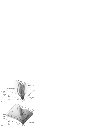
Figure 1: The correction factor to exact (a) and approximate (b) expressions for the maximum growth rate obtained within hydrodynamic or kinetic approximations.

At arbitrary $\tilde{n}_{b}$ and ${\scriptstyle\Delta}\tilde{v}$, we solve equation (2) numerically to yield the functions $\omega_{r}(\tilde{k})$ and $\gamma(\tilde{k})$, as well as the dependence of the maximum growth rate $\gamma_{m}=\gamma(\tilde{k}_{m})$ and its location $\tilde{k}_{m}$ on the beam parameters $\tilde{n}_{b}$ and ${\scriptstyle\Delta}\tilde{v}$. The function $\gamma_{m}(\tilde{n}_{b},{\scriptstyle\Delta}\tilde{v})$ itself is not very informative, so we plot in Fig. 1a the correction factor $\kappa$, the ratio of the exact $\gamma_{m}$ to the maximum growth rate obtained by solving Eq.(5) or maximization of (8), whichever gives better approximation. For comparison, in Fig. 1b there is a ratio of $\tilde{\gamma}_{m}$ to approximations of the maximum growth rate given by (6) or (9), whichever is better. We see that, in a wide parameter area, the simple formulae (6) and (9) are only order-of-magnitude correct, while unabridged hydrodynamic and kinetic models give reasonably good approximations within their applicability areas. It should be particularly emphasized that the key simplifying assumptions used in unabridged hydrodynamic or kinetic models lead to overstatement of the growth rate which amounts to factor of two in the transition region.

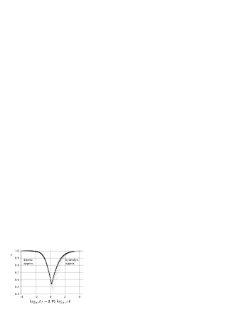
Figure 2: Dependence of the correction factor $\kappa$ on the combined beam parameters for $1>{\scriptstyle\Delta}\tilde{v}>0.01$. The black points correspond to $10^{-2}>\tilde{n}_{b}>10^{-4}$; the grey points, $1>\tilde{n}_{b}>0.01$.

Surprisingly, the “valley” in Fig. 1a is straight and has an invariable cross-section. Thus, with a good precision, we may assume that the beam parameters enter the function $\kappa(\tilde{n}_{b},{\scriptstyle\Delta}\tilde{v})$ only as a combination $\tilde{n}_{b}{\scriptstyle\Delta}\tilde{v}^{-s}$, with $s\approx 3.15$ found empirically. The dependence of the correction factor $\kappa$ on the difference of decimal logarithms $\log_{10}\tilde{n}_{b}-s\log_{10}{\scriptstyle\Delta}\tilde{v}$ is shown in Fig. 2.

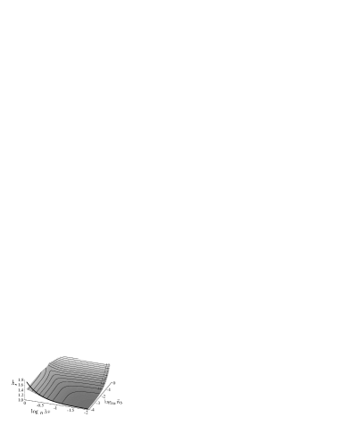
Figure 3: Wavenumber $\tilde{k}_{m}$ of the most unstable wave. The thick line shows the scaling (9).

For $\tilde{n}_{b}\ll 0.1$, the wavenumber $\tilde{k}_{m}$ of the most unstable mode does not depend on the beam density, follows the kinetic formula remarkably well, and, at ${\scriptstyle\Delta}\tilde{v}\ll 1$, can be safely approximated by (9) (Fig. 3). As the beam density approaches the plasma density, $\tilde{k}_{m}$ tends to $\sqrt{3}$, the value found for equal counterstreaming electron flows Mikh .

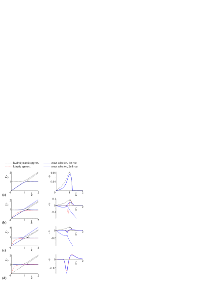
Figure 4: (Color online) Evolution of dispersion curves: numerical solution to the full dispersion relation (2) (solid lines), numerical solution to hydrodynamic dispersion relation (5) (dotted lines), and kinetic expressions (7) and (8) (dashed lines): real part $\tilde{\omega}_{r}(\tilde{k})$ (left column) and growth rate $\tilde{\gamma}(\tilde{k})$ (right column). Beam density $\tilde{n}_{b}=0.002$, beam velocity spread: (a) ${\scriptstyle\Delta}\tilde{v}=0.05$ (nearly hydrodynamic regime), (b) ${\scriptstyle\Delta}\tilde{v}=0.12$ (the greatest difference between maximum growth rates), (c) ${\scriptstyle\Delta}\tilde{v}=0.24$ (close to reconnection of dispersion curves), and (d) ${\scriptstyle\Delta}\tilde{v}=0.3$ (nearly kinetic regime).

It is interesting to follow evolution of exact and approximate dispersion curves as we travel in the parameter space from the hydrodynamic regime to the kinetic one. For this, we put $\tilde{n}_{b}=0.002$ and change ${\scriptstyle\Delta}\tilde{v}$ (Fig. 4). As ${\scriptstyle\Delta}\tilde{v}$ increases, the growth rate decreases (Fig. 4a), the instability interval shifts to greater values of $\tilde{k}$ and narrows, while the real part of the frequency changes insignificantly (Fig. 4b). At some value of ${\scriptstyle\Delta}\tilde{v}$ (when the growth rate already approaches the value given by the kinetic approximation), a reconnection of dispersion curves takes place (Fig. 4c) PF11-1754 ; JGR94-2429 , after which both real and imaginary parts of the wave frequency closely follows the kinetic formulae (7) and (8).

This work is supported by RF President’s grants NSh-2749.2006.2 and MD-4704.2007.2, RFBR grants 06-02-1657 and 08-01-00622, and Russian Ministry of Education (projects RNP 2.2.1.1.3653 and innovation educational project 456).

References

- (1) R. Briggs, in Advances in Plasma Physics, edited by A. Simon and W. B. Thompson (Interscience, New York, 1971), Vol. 4, p. 43.
- (2) N. A. Krall and A. W. Trivelpiece, Principles of Plasma Physics (McGraw-Hill, New York, 1973).
- (3) A. B. Mikhailovskii, Theory of Plasma Instabilities (Consultants Bureau, New York, 1974), Vol. 1.
- (4) A. A. Ivanov, Physics of Highly Nonequilibrium Plasma. (Atomizdat, Moscow, 1977) [in Russian].
- (5) A. Burdakov, A. Azhannikov, V. Astrelin, et al., Transactions of Fusion Science and Technology 51, 106 (2007).
- (6) A. V. Arzhannikov, V. T. Astrelin, A. V. Burdakov, et al., Plasma Physics Reports 31, 462 (2005).
- (7) A. V. Arzhannikov, V. T. Astrelin, A. V. Burdakov, I. A. Ivanov, V. S. Koidan, K. I. Mekler, V. V. Postupaev, A. F. Rovenskikh, S. V. Polosatkin, and S. L. Sinitskii, JETP Lett. 77, 358 (2003).
- (8) I. V. Timofeev and K. V. Lotov, Phys. Plasmas 13, 062312 (2006).
- (9) A. A. Galeev and R. Z. Sagdeev, in Reviews of Plasma Physics, edited by M. A. Leontovich (Consultants Bureau, New York, 1979), Vol. 7, p. 1.
- (10) T. M. O’Neil and J. H. Malmberg, Phys. Fluids 11, 1754 (1968).
- (11) C. T. Dum, Journal of Geophysical Research 94, 2429 (1989).
- (12) V. D. Shafranov, in Reviews of Plasma Physics, edited by M. A. Leontovich (Consultants Bureau, New York, 1967), Vol. 3, p. 1.