A boundary integral formalism for stochastic ray tracing in billiards

Abstract

Determining the flow of rays or particles driven by a force or velocity field is fundamental to modelling many physical processes, including weather forecasting and the simulation of molecular dynamics. High frequency wave energy distributions can also be approximated using flow or transport equations. Applications arise in underwater and room acoustics, vibro-acoustics, seismology, electromagnetics, quantum mechanics and in producing computer generated imagery. In many practical applications, the driving field is not known exactly and the dynamics are determined only up to a degree of uncertainty. This paper presents a boundary integral framework for propagating flows including uncertainties, which is shown to systematically interpolate between a deterministic and a completely random description of the trajectory propagation. A simple but efficient discretisation approach is applied to model uncertain billiard dynamics in an integrable rectangular domain.

Many physical transport problems can be formulated in terms of ray tracing or trajectory methods. Applications range from particle tracking in fluids [1, 2] and the simulation of molecular dynamics [3] to illumination and rendering problems in computer graphics [4] or, more generally, the geometric optics limit of linear wave equations. A range of techniques have been developed for solving ray tracing problems. One distinguishes between direct ray-tracing [5, 6] based on following ray paths from a source to receiver point and variants thereof; and indirect methods using transport equations based on conservation laws such as the Liouville equation [7] to propagate phase space densities. In the latter case one arrives at a model for propagating phase-space densities using deterministic transfer operators of the Frobenius-Perron (FP) type [8]. In this paper we will introduce a new boundary integral method for determining phase-space densities propagated via a stochastic trajectory flow using a transfer operator approach.

1 Introduction

A variety of techniques have emerged recently with the aim of turning transfer operators into an efficient numerical tool for practical applications. Domain based transfer operator approaches, for example, start by subdividing the phase-space into distinct cells and considering transition rates between these phase-space regions. One of the simplest and most common approaches of this type is Ulam’s method (see e.g. [9]). Other methods include wavelet and spectral methods for the infinitesimal FP-operator [10, 11], eigenfunction expansion methods [12] and periodic orbit expansion techniques [8, 13]. Also the modelling of many-particle dynamics, such as protein folding, has been approached using short trajectories of the full, high-dimensional molecular dynamics simulation to construct reduced Markov models [3]. For a discussion of convergence properties of the Ulam method in one and several dimensions, see [14] and [15], respectively. However, such methods have only found a fairly limited range of applicability, with difficulties arising due to the high-dimensionality of the phase-space.

In the following we will focus on integral equation formulations for propagating phase space densities along ray trajectories using transfer operators. One such formulation is given by the rendering equation [4] which has its origins in computer graphics, but has been applied more widely since [16, 17]. The rendering equation can again be formulated in terms of transfer operators [17, 18]. A boundary integral FP-operator approach called dynamical energy analysis (DEA) has been introduced in [17] and further developed in [19]. In a sequence of papers [20, 21] the method has evolved into an mesh-based tool called discrete flow mapping (DFM) described in [22, 23]. This has proven to be an efficient numerical tool making it possible to handle trajectory flow problems on complex surfaces (consisting of circa $10^{5}$ to $10^{6}$ mesh cells) on the time-scale of a few hours on standard desktop computers [23].

Here we will extend the DEA approach towards dynamical systems with uncertainties and stochastic dynamics. The reasons for doing so are twofold: firstly, in many physically relevant situations, the system dynamics are inherently stochastic or system parameters are not known exactly and a probabilistic approach will be necessary. Secondly, including stochasticity in a transfer operator changes the properties of the operator fundamentally in a way that opens the door for a wider range of numerical solution techniques. Techniques for constructing stochastic ray-tracing operators have been presented in [24, 25, 26, 27] in the context of the FP operator, and in acoustics in terms of the radiosity equation [28].

In this paper we construct a stochastic ray-tracing operator that leads to a boundary integral formulation for stochastic dynamics in billiards. That is, the underlying dynamical system is that of a particle or point mass moving on a billiard table with constant velocity (without friction) inside a compact domain $\Omega$ with piecewise smooth boundary $\Gamma$ as described by Sinai [29], see also [8], Ch. I, Sec. 8. The particle is assumed to undergo specular reflections upon collision with the smooth sections of $\Gamma$. As the overall energy of the system is constant, the billiard dynamics (integrable, mixed or chaotic) is completely controlled by the geometry of $\Gamma$. However, for the stochastic evolution considered here, both the position of the transported particle and the nature of its reflection at the boundary will be considered as uncertain. Typically, the mean transported position and reflected direction will be those of the standard (deterministic) billiard map. The effect is that total energy remains constant, but the stochasticity will clearly influence the billiard dynamics as will be explored in Section 3.3. The resulting stochastic evolution operator will be of Fokker-Planck type as discussed in [13, 24].

We note that statistical methods related to the stochastic approach proposed here have been used in a variety of engineering applications. In particular, the so-called statistical energy analysis (SEA) (see for example [30] and [31]) for modelling vibro-acoustic energy distributions and the random coupling model (RCM) [32] for modelling electromagnetic fields, see also [33]. In SEA and RCM the structure is subdivided into a set of subsystems and ergodicity of the underlying ray dynamics as well as quasi-equilibrium conditions are postulated. The result is that the density in each subsystem is taken to be approximately constant leading to greatly simplified equations based only on coupling constants between subsystems. The disadvantage of these methods is that the underlying assumptions are often hard to verify a priori or are only justified when an additional averaging over ‘equivalent’ subsystems is considered. The shortcomings of SEA have been addressed by Langley [34, 35] and more recently in a series of papers by Le Bot [16, 28, 36].

In this work we focus on stochastic ray-tracing approximations for linear wave problems in two-dimensions, or equivalently on stochastic billiard dynamics; the models developed can easily be generalized to higher dimensions. We propose a new boundary integral approach based on the use of stochastic evolution operators to incorporate uncertain ray dynamics into our model in a quantifiable manner. Propagating densities with uniformly distributed probability of location and direction leads to the quasi-equilibrium approaches mentioned above (SEA and RCM). We will show that choosing a scaled and truncated Gaussian probability distribution instead leads to a model that interpolates between SEA and deterministic ray tracing. This interpolation takes place at the level of the governing model, in contrast to DEA which provides a similar interpolation due to the precision of the chosen numerical approximation method [17]. Once an estimate of the level of uncertainty in the model has been prescribed, an appropriate numerical solution approach can be applied.

The paper is structured as follows: in Sec. 2 a boundary integral description of deterministic ray tracing in billiards will be presented. The addition of noise into the model will then be outlined and an approach that interpolates between a deterministic and a random trajectory flow will be described. In Sec. 3, the numerical implementation of the model will be outlined and illustrated via the example of stochastic ray tracing in a rectangular billiard. The decay of correlations and the asymptotic escape rate will be studied to diagnose the behaviour of the rectangular billiard model as it makes the transition from regular and deterministic to probabilistic dynamics.

2 Boundary Integral Equation Formulation

2.1 A boundary integral description of deterministic ray tracing via transfer operators

Consider the trajectory flow described by a Hamiltonian $\hat{H}=c|\mathbf{p}|$ in a finite two-dimensional domain $\Omega$ as depicted in Fig. 1, where $c$ is the speed of propagation and $\mathbf{p}$ is the inward momentum (or slowness) vector. Denote the phase-space on the boundary of $\Omega$ with fixed total energy $\hat{H}=1$ as $Q=\Gamma\times(-c^{-1},c^{-1})$, where $\Gamma$ is the boundary of $\Omega$. The associated coordinates are $X=[s,\>p]\in Q$ with $s\in[0,L)$ (arc-length) parameterising $\Gamma$ and $p\in(-c^{-1},c^{-1})$ parameterising the component $\mathbf{p}$ tangential to $\Gamma$. Explicitly, the momentum coordinate $p$ is defined in terms of the angle $\theta$ between $\mathbf{p}$ and the normal to $\Gamma$ at $s$ (see Fig. 1) as $p=c^{-1}\sin(\theta)$. We adopt the convention that $\theta\in(-\pi/2,\pi/2)$ and is positive for counter-clockwise propagation. The deterministic boundary flow map is denoted $\varphi:Q\rightarrow Q$, and maps a vector in $Q$ via the Hamiltonian flow to another vector in a subset of $Q$. This map defines a deterministic evolution of the form $\varphi(X^{\prime})=X$, where $X^{\prime}=[s^{\prime},\>p^{\prime}]$, $X=[s,p]$ . Fig. 1 shows that geometrically $\varphi$ corresponds to the composition of a translation (from $s^{\prime}$ to $s$) and a rotation to the direction corresponding to a specular reflection.

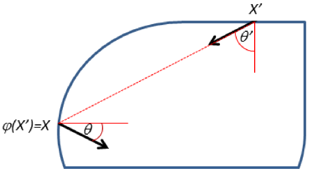
Figure 1: Propagation of ray trajectories using a deterministic boundary map.

The propagation of a phase-space density $\rho$ by the boundary map $\varphi$ through a single reflection is given by the Frobenius-Perron operator acting on this map

$$\mathcal{L}\rho(X)=\int_{Q}\delta(X-\varphi(X^{\prime}))\rho(X^{\prime})dX^{\prime}.$$ (1)

For an initial boundary distribution $\rho_{0}$ on $Q$, the final density after adding contributions from all refections may be computed using the following boundary integral equation (see [17], [20] and [21]),

$$(I-\mathcal{L})\rho=\rho_{0}.$$ (2)

Note that for the sum over all reflections to converge, energy losses must be introduced into the system, which could take place at the boundaries themselves, or along the trajectories. In general, a weight factor $w$ will be added inside the integral in the definition of $\mathcal{L}$ which contains a dissipative term, and for the extension to multiple domains connected at interfaces $w$ will also contain reflection/transmission probabilities at these interfaces. For non-convex polygons, $w$ will additionally include a visibility function.

2.2 Stochastic trajectory tracking in billiards

2.2.1 The stochastic propagation operator

Building upon the deterministic propagation models described in the previous section, we propose a family of phase space density propagation models with transfer operators of the form

$$\mathcal{L}_{\boldsymbol{\sigma}}\rho(X)=\int_{Q}f_{\boldsymbol{\sigma}}(X-\varphi(X^{\prime}))\rho(X^{\prime})dX^{\prime}.$$ (3)

This operator bears a strong similarity to (1), but the $\delta$ distribution term has been replaced with a probability density function (PDF) $f_{\boldsymbol{\sigma}}$ such that

$$\int_{Q}f_{\boldsymbol{\sigma}}(X)dX=1.$$ (4)

Here, $f_{\boldsymbol{\sigma}}$ is the probability distribution and $\boldsymbol{\sigma}$ is the parameter set controlling its shape. With reference to applications, such a probabilistic behaviour could be attributed to, for example, fluctuations in the wave speed $c$, roughness of the reflecting surface or uncertainty in the exact position of the boundary. In the following, we will always assume that the total energy $\hat{H}=c|\mathbf{p}|=1$ remains fixed and that the total probability is conserved, that is, condition (4) holds throughout. Note that in contrast to the models considered in [13, 24], the range of integration in the billiard models considered here is in general bounded, which has implications for the choice of suitable PDFs $f_{\boldsymbol{\sigma}}$.

The simplest case is to take $f_{\boldsymbol{\sigma}}=const$, upon which one arrives at a model describing propagation to all admissible positions and directions with equal probability. The systems is thus by definition ergodic and independent of the underlying classical dynamics. Note that ergodicity is a key assumption for an SEA or RCM treatment to be valid.

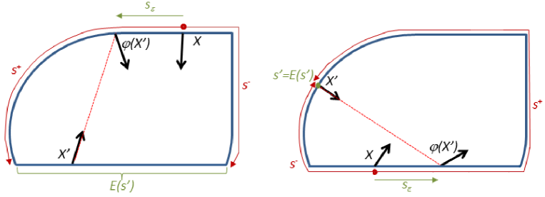
Figure 2: Tracking ray trajectories via a noisy boundary map and truncation limits $s^{\pm}$ for the random variable $s_{\varepsilon}$.

In general, we would like to arrive at a stochastic operator which includes both the deterministic operator in Eq.  (1) and the random propagation model described above as limiting cases. In addition, the PDF $f_{\boldsymbol{\sigma}}$ needs to obey conditions on the sampling ranges due to the limited range of the boundary map $\varphi$. For simplicity we will restrict to convex domains $\Omega$ to avoid additional complications due to incorporating visibility functions.

2.2.2 The probability density function - normalisation

We may interpret the evolution given by the operator in Eq. (3) as originating from a stochastic boundary map $\varphi_{\boldsymbol{\sigma}}$ with added noise, that is,

$$\begin{split}\varphi_{\boldsymbol{\sigma}}(X^{\prime})&={X},\\ &=\varphi(X^{\prime})+X_{\varepsilon},\end{split}$$ (5)

where $X_{\varepsilon}=[s_{\varepsilon},p_{\varepsilon}]$ are random variables drawn from the PDF $f_{\boldsymbol{\sigma}}$. Note that $s_{\varepsilon}$ is understood as a shift in counter-clockwise direction. For $X\in Q$ given, we have to ensure that $\varphi(X^{\prime})=X-X_{\varepsilon}$ is still in the range of the deterministic map $\varphi$; this yields restrictions on the possible values of $X_{\varepsilon}$ and thus on the domain of $f_{\boldsymbol{\sigma}}$.

We define $\varphi=[\varphi_{s},\>\varphi_{p}]$ in terms of its position and momentum components and write the initial coordinate as $X^{\prime}=[s^{\prime},p^{\prime}]$. The range of admissible values for $\varphi_{s}(X^{\prime})$ is $[0,L)\setminus E(s^{\prime})$, where $E(s^{\prime})$ is the (closed) set of all points on the same straight edge as $s^{\prime}$, see Fig. 2. Note that for curved edges we set $E(s^{\prime})=s^{\prime}$ as shown on the RHS of Fig. 2. Furthermore, we have that $\varphi_{p}(X^{\prime})\in(-c^{-1},c^{-1})$. It is therefore necessary to truncate the ranges from which $X_{\varepsilon}$ are sampled to the ranges where for fixed $X$, $\varphi(X^{\prime})\in([0,L)\setminus E(s^{\prime}))\times(-c^{-1},c^{-1})$ in Eq. (5). Denoting these truncated ranges by $(X^{-},X^{+})$ where $X^{\pm}=[s^{\pm},\>p^{\pm}]$, the PDF $f_{\boldsymbol{\sigma}}$ will have support on $X_{\varepsilon}\in(X^{-},X^{+})$ only. The truncated sampling ranges are given as $s^{+}(s^{\prime},s)=\min\{x>0:s+x\in{E}(s^{\prime})\>\>(\mathrm{mod}\>L)\}$ and correspondingly $s^{-}(s^{\prime},s)=\max\{x<0:s+x\in{E}(s^{\prime})\>\>(\mathrm{mod}\>L)\}$ (see Fig. 2). Likewise in the momentum coordinate, $p^{+}(p)=c^{-1}-p$ and $p^{-}(p)=-c^{-1}-p$. Using Heaviside functions we define a cut-off function for restricting the support of $f_{\boldsymbol{\sigma}}$ to $(X^{-},X^{+})$ as follows

$$\begin{split}&\chi(X_{\varepsilon};X^{-},X^{+})\\ &=(H(s^{+}-s_{\varepsilon})-H(s^{-}-s_{\varepsilon}))(H(p^{+}-p_{\varepsilon})-H(p^{-}-p_{\varepsilon})).\\ \end{split}$$ (6)

Note that we have omitted the dependence of $s^{\pm}$ and $p^{\pm}$ on $X^{\prime}$ and $X$ for brevity.

Having obtained the domain of the PDF, we can now construct $f_{\boldsymbol{\sigma}}$ explicitly; we will derive the PDF from an uncorrelated bivariate Gaussian distribution with mean $\mathbf{0}=[0,0]$ and standard deviation $\boldsymbol{\sigma}=[\sigma_{1},\sigma_{2}]$. A normalized PDF is then obtained by setting

$$f_{\boldsymbol{\sigma}}(X_{\varepsilon};X^{-},X^{+})=\frac{\chi(X_{\varepsilon};X^{-},X^{+})\exp{\left(\displaystyle-\frac{s_{\varepsilon}^{2}}{2\sigma_{1}^{2}}\right)}\exp{\left(\displaystyle-\frac{p_{\varepsilon}^{2}}{2\sigma_{2}^{2}}\right)}}{2\pi\sigma_{1}\sigma_{2}\psi_{\sigma_{1}}(s^{-},s^{+})\psi_{\sigma_{2}}(p^{-},p^{+})},$$ (7)

where the normalization defined through $\psi_{\sigma_{1}}$ and $\psi_{\sigma_{2}}$ is given as

$$\psi_{\sigma_{1}}(s^{-},s^{+})=\frac{1}{2}\left(\mathrm{erf}\left(\frac{s^{+}}{\sqrt{2}\sigma_{1}}\right)-\mathrm{erf}\left(\frac{s^{-}}{\sqrt{2}\sigma_{1}}\right)\right),$$ (8)

and $\psi_{\sigma_{2}}$ is defined analogously. The normalisation ensures that the PDF satisfies condition (4) for the truncated sampling ranges specified through $\chi$. Note that the mean and variance of $f_{\boldsymbol{\sigma}}$ differs in general from that of the underlying Gaussian distribution.

The two limiting PDFs are obtained by considering the limiting values of ${\boldsymbol{\sigma}}$. Taking the limit of (7) as $\boldsymbol{\sigma}\rightarrow\mathbf{0}$ then

$$f_{\boldsymbol{\sigma}}(X_{\varepsilon};X^{-},X^{+})\rightarrow\lim_{\boldsymbol{\sigma}\rightarrow\mathbf{0}}\frac{\chi(X_{\varepsilon};X^{-},X^{+})}{2\pi\sigma_{1}\sigma_{2}}\exp{\left(\displaystyle-\frac{s_{\varepsilon}^{2}}{2\sigma_{1}^{2}}\right)}\exp{\left(\displaystyle-\frac{p_{\varepsilon}^{2}}{2\sigma_{2}^{2}}\right)}.$$ (9)

The distribution becomes increasingly sharp and the bivariate Gaussian tends to a two-dimensional delta distribution localised around $X_{\varepsilon}=X-\varphi(X^{\prime})=0$, which describes the deterministic flow discussed in the Section 2.1. Taking the limit as $\sigma_{1}$, and $\sigma_{2}$ go to $\infty$ and using the leading order asymptotic expansion of the error function about 0 returns

$$f_{\boldsymbol{\sigma}}(X_{\varepsilon};X^{-},X^{+})\rightarrow\frac{c}{2(s^{+}-s^{-})}\chi(X_{\varepsilon};X^{-},X^{+}).$$ (10)

Note that this is just the uniform distribution for $s_{\varepsilon}\in(s^{-},s^{+})$ and $p_{\varepsilon}\in(p^{-},p^{+})$ (since $p^{+}-p^{-}=2c^{-1}$) leading to the fully probabilistic regime described above. The mean and variance of the normalized distribution may be calculated from the PDF (7) using the standard formulae. The variance of the bivariate distribution will tend to $\boldsymbol{\sigma}$ as $\boldsymbol{\sigma}\rightarrow\mathbf{0}$. For large $\sigma_{j}$, $j=1,2$ we have the variance of the uniform distribution. That is, as $\sigma_{1}\rightarrow\infty$, $\mathrm{Var}(s_{\varepsilon})=(s^{+}-s^{-})^{2}/12$, and as $\sigma_{2}\rightarrow\infty$, then $\mathrm{Var}(p_{\varepsilon})=1/(3c^{2})$. Clearly such data are vital for applications in uncertainty quantification, for example, for modelling uncertain high frequency vibro-acoustic or electromagnetic wave propagation through a manufactured structure or device.

We turn our attention to propagating a density along stochastic ray paths according to the PDF (7) via the transfer operator (3). We proceed by considering the numerical evaluation of $\mathcal{L}_{\boldsymbol{\sigma}}$; we will in particular consider some important dynamical quantities, namely the rate of escape and the decay of correlations. These will be studied to help diagnose the behaviour of the model for different ranges of $\boldsymbol{\sigma}$.

3 Implementation and Results

3.1 Discretisation

A number of efficient methods for evaluating $\mathcal{L}$ numerically in domains including complex multi-component systems have recently been developed [22, 23]. One advantage of instead working with $\mathcal{L_{\boldsymbol{\sigma}}}$ is that it is a compact integral operator and hence may be evaluated more simply via direct discretisation methods rather than the variational approaches described in [22, 23] and references therein.

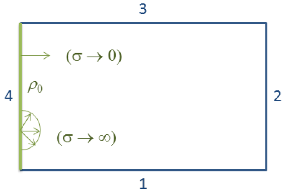
Figure 3: A rectangular billiard with prescribed boundary condition $\rho_{0}$.

Here we approximate $\mathcal{L}_{\boldsymbol{\sigma}}$ on a rectangular billiard as shown in Fig. 3. The reason for choosing this simple domain is that its integrable dynamics make it ideal for identifying the effect of varying $\boldsymbol{\sigma}$ in isolation of other sources of ray chaotic behaviour. In particular, we make use of our experience in dealing with domains with corners in [22, 23] and employ a piecewise constant collocation method with $n$ elements in the position variable, collocating at element centers. That is, we separate out and approximate the spatial dependence of $\rho$ in the form

$$\rho(s,p)\approx\tilde{\rho}(p)\sum_{j=1}^{n}a_{j}b_{j}(s),$$ (11)

where $b_{j}(s)=1$ if $s$ lies on the $j$th element and zero elsewhere. The coefficients $a_{j}$ are the unknowns to be determined. The semi-discrete operator $\mathcal{L}_{\sigma}$ is then evaluated at the collocation points $s=s_{i}$ for $i=1,\ldots,n$ using equation (3) as

$$\mathcal{L}_{\boldsymbol{\sigma}}\rho(s_{i},p)=\sum_{j=1}^{n}a_{j}\int_{-c^{-1}}^{c^{-1}}\tilde{\rho}(p^{\prime})\int_{e_{j}}f_{\boldsymbol{\sigma}}(X_{i}-\varphi(X^{\prime}))ds^{\prime}dp^{\prime},$$ (12)

where $X_{i}=[s_{i},\>p]$ and the range of integration with respect to $s^{\prime}$ is on the $j$th element $e_{j}$. The phase space coordinate $X^{\prime}=[s^{\prime},\>p^{\prime}]$ provides the variables integration $s^{\prime}\in e_{j}$ and $p^{\prime}\in(-c^{-1},c^{-1})$. Note that the integral with respect to $s^{\prime}$ may be calculated analytically in terms of the error function for discretisation by flat (straight line) elements and using the normalised PDFs described in the last section. This step is important for efficient computations of the discretised transfer operator.

A full discretisation is then achieved by applying the Nyström method in momentum space with $N$-point trapezoidal integration and a step size $h$. Note that in order to evenly discretize with respect to the direction of ray propagation, the integration variable is changed from $p^{\prime}$ to $\theta^{\prime}$ using the relation $cp^{\prime}=\sin(\theta^{\prime})$. This reduces the calculation in (12) to a matrix-vector multiplication, with matrix entries of the form

$$L_{I,J}=\frac{h\cos(\theta^{\prime})}{c}\int_{e_{j}}f_{\boldsymbol{\sigma}}(X_{I}-\varphi(X_{J}^{\prime}))ds^{\prime}.$$ (13)

Here $X_{I}=[s_{i},\>p_{\iota}]$ and so $I$ is the multi-index $(i,\>\iota)$, with $p_{\iota}$, $\iota=1,\ldots,N$ giving the values of the momenta corresponding to the trapezoidal rule grid points. Likewise, $X_{J}^{\prime}=[s^{\prime},\>p_{k}]$ and $J$ is the multi-index $(j,\>k)$, where $s^{\prime}\in e_{j}$ is the integration point and $p_{k}$, $k=1,\ldots,N$ runs over the trapezoidal rule grid points as before. The density $\rho$ can (by extension) be considered as periodic in the momentum variable since $\rho(s,c^{-1})=\rho(s,-c^{-1})=0$, and so the semi-discretisation in momentum space should converge super-algebraically for smooth initial data. The convergence properties of the method overall are demonstrated in the next section. A further major advantage of this combination of methods is that the need for numerical integration methods is completely avoided.

3.2 Convergence

To test the convergence of the approximation of $\mathcal{L}_{\boldsymbol{\sigma}}$ we propagate a stochastic boundary (line) source through a single reflection. The dimensions of the rectangle are taken to be $0.75$ by $0.25$ and we let $c=1$ meaning that both the position and momentum variables have the same total range. We also take $\sigma_{1}=\sigma_{2}=\sigma$ for simplicity, although the extension to distinct $\sigma_{1}$ and $\sigma_{2}$ is clearly straightforward. We number the edges as shown in Fig. 3 so that edges $1$ and $3$ have length $0.75$ and take

$$\rho_{0}(s,p)=\frac{I_{4}(s)\exp\left(\displaystyle\frac{-p^{2}}{2\sigma^{2}}\right)}{\sqrt{2\pi\sigma^{2}}\mathrm{erf}\left(\frac{1}{\sqrt{2}\sigma}\right)},$$ (14)

where $I_{4}$ is an indicator function for edge number 4. That is, the source is applied along edge 4 as shown in Fig. 3 and its directivity depends on the parameter $\sigma$. Figure 4 shows the result of approximating $\mathcal{L}_{\sigma}\rho_{0}$ on sides 1 to 3 of the rectangle. The plot shows the mean ray density along each of the 3 edges plotted against the outgoing angle. The horizontal axis is a shifted value of this outgoing angle which is unshifted on side 1, shifted by $\pi$ on side 2 and by $2\pi$ on side 3. This is simply to show the results for each edge side-by-side.

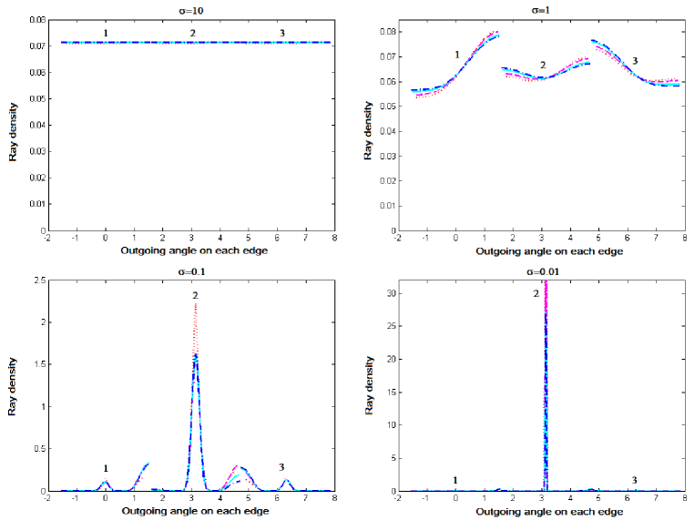
Figure 4: Convergence of the ray density after one reflection and the effect of changing $\sigma$ on the dynamics. For all plots except $\sigma=0.01$: $\cdots$: $N=16$, $--$: $N=32$, —: $N=64$, $\cdot$-$\cdot$: $N=128$. For the $\sigma=0.01$, the previous $N$ values should all be multiplied by 4. The horizontal axis shows the outgoing angle in the range $-\pi/2$ to $\pi/2$ on edge 1, on edge 2 it is shifted by $\pi$ and on edge 3 it is shifted by $2\pi$. Edge numbers are indicated on the plot.

Figure 4 shows the transition from probabilistic to deterministic dynamics as $\sigma$ is decreased, and therefore illustrates the theory outlined in the Section 2.2. In particular, for $\sigma=10$ we see a uniformly distributed ray density across all edges and all outgoing directions. For $\sigma=0.01$ one sees that the ray density localises on edge 2 with outgoing angle 0, i.e. perpendicular to the boundary. This is a close approximation to the expected deterministic evolution. The intermediate cases ($\sigma=1$ and $\sigma=0.1$) show the transition between these two limiting cases. This transition will be considered in more depth in the next section.

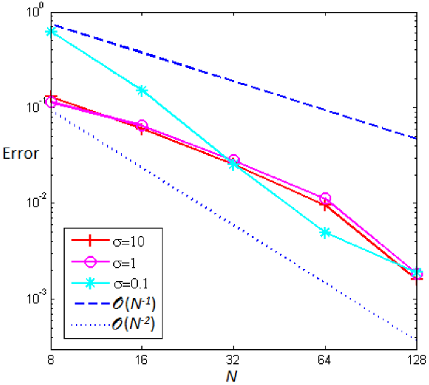
Figure 5: Convergence rate in computing the total ray density (15) for different values of $\sigma$.

In order to test the convergence of the results shown in Figure 4, we integrate the boundary phase-space density over $Q$ to estimate the total density

$$\rho_{\mathrm{tot}}=\int_{Q}\mathcal{L}_{\boldsymbol{\sigma}}\rho_{0}dX.$$ (15)

For the basic discretisation approaches employed here and taking $n=N$ one typically sees convergence in computing $\rho_{\mathrm{tot}}$ to the first few significant figures with absolute errors of estimated order between $\mathcal{O}(N^{-1})$ and $\mathcal{O}(N^{-2})$ as shown in Figure 5. Note that these rates appear to be superior to the sub-linear rates expected from a standard Ulam approach [14]. Convergence rates are generally higher for smaller values of $\sigma$, and usually increase slightly when the number of discretisation points $n=N$ in both the position and momentum variables is increased. Note that for $\sigma=0.01$, the method has only converged sufficiently to produce meaningful results when $N\geqslant 128$ and as such this case has been omitted from the figure. This suggests that the singularly perturbed problem for small $\sigma$ should be tackled using an adaptive meshing procedure to resolve the peak(s) more efficiently, rather than the uniform grid employed here. The development and analysis of such approaches will be considered as part of future work.

3.3 Rate of escape and decay of correlations

The rates of escape and decay of correlation provide useful information about the dynamics of the billiard system being studied in terms of their description and classification (chaotic, mixed or integrable). The escape rate $\gamma$ measures the decay of the total phase space density, that is, the survival probability, in case of an open or absorbing billiard. This decay is exponential for chaotic dynamics, that is,

$$\int_{Q}\left[{\cal L}^{n}_{\sigma}\rho_{0}\right](X)\;dX\sim e^{-\gamma n};$$

similarly, for closed, chaotic systems, the decay of correlation scales exponentially with a decay rate $\nu$ according to

$$\int_{Q}\rho_{0}(X)\left[{\cal L}^{n}_{\sigma}\rho_{0}\right](X)\;dX-\left[\int_{Q}\rho_{0}(X)\overline{\rho}(X)\;dX\right]^{2}\sim e^{-\nu n},$$

where $\overline{\rho}=\lim_{n\to\infty}{\cal L}_{\sigma}^{n}\rho_{0}$ is the natural density (if the limit exists). Both, $\gamma$ and $\nu$ are closely linked to the spectrum of ${\cal L_{\sigma}}$ with $\exp(-\gamma)$ and $\exp(-\nu)$ being the magnitude of the leading and next-leading eigenvalue of ${\cal L_{\sigma}}$ for ergodic dynamics [8].

The rates $\gamma,\nu$ are also important when considering wave energy propagation through a built up structure [37]. In particular, the suitability of the random wave superposition hypothesise of an SEA-type approach can be analysed in this framework, since a fast decay of correlations compared to the escape rate provide the ideal setting for a diffuse random wave field to be created [17]. On the other hand, slow or non-decaying correlations in the dynamics indicate regularity in the wave field and will introduce non-random fluctuations and potentially long range correlations between multiple sub-domains.

In this section we study the decay of correlations in the rectangular billiard described earlier for different choices of the parameter $\sigma$. In addition, we consider the rate of escape when a small opening is introduced on the boundary and consider the effect of changing both $\sigma$ and the size of the opening.

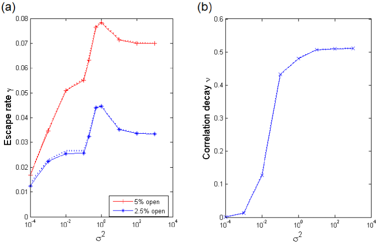
Figure 6: (a) The dependence of the asymptotic escape rate on $\sigma^{2}$ in a rectangular billiard for two different hole sizes. (b) The dependence of the decay of correlations on $\sigma^{2}$ in a closed rectangular billiard. In each case the dotted lines show the same quantities as the solid lines, but computed using half number of discretisation points for both $n$ and $N$.

Figure 6 (a) shows a plot of the asymptotic escape rate $\gamma$ against $\sigma^{2}$, where the escape rate is given by minus the logarithm of the spectral radius of the (numerical approximation to the) operator $\mathcal{L}_{\sigma}$. In each case the opening is on edge 2, and the two plots shown are for openings of size $0.05$ (from $y=0.1$ to $0.15$) and $0.1$ (from $y=0.15$ to $0.25$). For large $\sigma$ values we see $\gamma$ settling down to a constant, the size of which is approximately proportional to the opening size. This would be expected, since for chaotic maps the asymptotic escape rate due to a small opening is an exponential decay which to leading order is proportional to the hole size (see for example [38], [39]). For small sigma values we see that the escape rate decreases towards zero. Again, this reflects the supporting theory since as the map approaches a deterministic billiard map in a rectangle, the integrable dynamics and “sticky” trajectories (small perturbations of the bouncing ball modes) slow the decay to an algebraic rate [40]. Such a decay would be reflected by $\mathcal{L}_{\sigma}$ having a spectral radius of $1$, and hence $\gamma\rightarrow 0$.

Figure 6 (b) shows a plot of the correlation decay rate $\nu$ against $\sigma^{2}$, which may also be estimated from the spectrum of the operator $\mathcal{L}_{\sigma}$. In this case we look at the size of the second largest eigenvalue $\lambda^{*}$ of the closed billiard (the largest eigenvalue is always one for a closed system). The plot shows $\nu=-\log(|\lambda^{*}|)$ increasing with $\sigma^{2}$. For very small $\sigma^{2}$ the plot shows an almost zero decay rate as would be expected for a system with deterministic and regular dynamics. For large $\sigma^{2}$ we see convergence to a value of just over $0.5$, which clearly indicates the stochastic behaviour introduced from the noise in the billiard flow. In fact, the dependence of the decay rate on $\sigma$ appears to follow two distinct behaviours. For $\sigma^{2}<0.1$ one sees a rapid increase of $\nu$ with $\sigma$, and for $\sigma^{2}>0.1$ the rate of increase is far slower. This can perhaps be attributed to the PDF governing the noise in the billiard flow. For $\sigma^{2}<0.1$, the noise added to the flow is closer to a non-correlated Gaussian distribution and for $\sigma^{2}>0.1$, the scaling and shifting become increasingly significant and the model approaches a uniform distribution.

Considering Figures 6 (a) and (b) together, a change of behaviour in the escape rate is also evident close to $\sigma^{2}=0.1$. Here the escape rate begins to increase more quickly before peaking just below $\sigma=1$, and then decreasing to a constant rate for $\sigma^{2}>10$. The behaviour for $0.1<\sigma^{2}<10$ indicates a transition region where the trajectory flow is not yet effectively random (uniformly distributed), but is also not behaving as a flow with uncorrelated Gaussian noise. The dotted lines in each case show a lower precision computation with $n$ and $N$ both halved. The similarities between the plots suggest a good level of convergence in the computations. This serves to highlight a further advantage of working with $\mathcal{L}_{\boldsymbol{\sigma}}$ rather than the FP operator, where such computations typically show little evidence of convergence [37].

4 Discussion and conclusions

A new boundary integral model to propagate ray densities via an uncertain trajectory flow has been presented. The resulting phase-space boundary integral representation reduces the dimensionality of the model, and was shown to directly interpolate between a deterministic and a random trajectory flow. The model was implemented numerically via a simple discretisation approach using piecewise constant collocation in space and a Nyström method in the momentum variable. Discrete flow mapping type methods were applied to give a highly efficient computational procedure. An application to uncertain billiard dynamics in an integrable rectangular domain was presented; the numerical results demonstrated the transition between a deterministic and a random flow. Using the rate of escape and the decay of correlations to further diagnose the behaviour of the model gave parameter ranges where the model was effectively behaving as a deterministic trajectory flow with a small amount of uncorrelated Gaussian noise, a random (uniformly distributed) flow and a transition phase in between.

In the future, the framework will be extended to three dimensional billiards by introducing the analog of the PDF (7) on the boundary surface and its corresponding hemispherical momentum space (see [20]). Practically one would have to also define an efficient discretisation scheme, but in principle similar methods to those here can be employed provided the closed boundary surface consists of (or can be well approximated by) a union of flat surfaces joined together at their edges. Such an extension would be important for applications in room acoustics.

A further natural extension arises since one could allow the parameters $\boldsymbol{\sigma}$ to depend on the phase space coordinate. In fact, since the PDF (7) already depends on the phase space point indirectly through dependence on $X^{\pm}$, this extension could be implemented directly in the model here without extra modification. On a practical note, the dependence of $\sigma_{1}$ on the spatial coordinate should to be assumed to be piecewise constant to match the collocation scheme and maintain the tractability of the integrals appearing in (13). This extension would be important for applications in computer graphics, where reflections may take place from surfaces with different properties. A further consideration here is that the methods also extend directly to built-up multi-component structures in the same way as DEA [19]. This opens up the formulation to applications to built-up vibro-acoustic structures and complex electromagnetic environments.

References

- [1] A. Celani, M. Cencini, A. Mazzino and M. Vergassola, “Active and passive fields face to face,” New Journal of Physics 6 72 (2004).
- [2] M. Sommer and S. Reich, “Phase-space volume conservation under space and time discretization schemes for the shallow-water equations,” Monthly Weather Review, 138, 4229-4236 (2010).
- [3] F. Noé, C. Schütte, E. Vanden-Eijnden, L. Reich and T.R. Weikl, “Constructing the equilibrium ensemble of folding pathways from short off-equilibrium simulations,” Proceedings of the National Academy of Sciences of the USA 106, 19011-19016 (2009).
- [4] J.T. Kayija, “The rendering equation,” in Proc. SIGGRAPH 1986: 143, DOI:10.1145/15922.15902 (1986).
- [5] M. Vorländer, “Simulation of the transient and steady-state sound propagation in rooms using a new combined ray-tracing/image-source algorithm,” J. Acoust Soc. Am. 86, 172-178 (1989).
- [6] V. Červený, Seismic ray theory (Cambridge University Press, Cambridge, UK, 2001).
- [7] R.J. LeVeque Numerical Methods for Conservation Laws, Lectures in Mathematics: ETH Zürich (Birkhäuser, Basel, Swizerland, 1992).
- [8] P. Cvitanović, R. Artuso, R. Mainieri, G. Tanner and G. Vattay Chaos: Classical and Quantum, ChaosBook.org (Niels Bohr Institute, Copenhagen, Denmark, 2012).
- [9] J. Ding and A. Zhou, “Finite approximations of Frobenius-Perron operators: A solution of Ulam’s conjecture to multi-dimensional transformations,” Physica D 92, 61-68 (1996).
- [10] O. Junge and P. Koltai, “Discretization of the Frobenius-Perron operator using a sparse Haar tensor basis - the Sparse Ulam method,” SIAM J. Num. Anal. 47, 3464-3485 (2009).
- [11] G. Froyland, O. Junge and P. Koltai, “Estimating long term behavior of flows without trajectory integration: the infinitesimal generator approach,” SIAM J. Num. Anal. 51(1), 223-247, (2013).
- [12] M. Budisic,́ R. Mohrand I. Mezic,́ “Applied Koopmanism,” Chaos 22, 047510 (2012).
- [13] D. Lippolis and P. Cvitanović, “How well can one resolve the state space of a chaotic map?” Phys. Rev. Lett., 104, 014101 (2010).
- [14] C.J. Bose and R. Murray, “The exact rate of approximation in Ulam’s method,” Discrete and Continuous Dynamical Systems 7 219-235 (2001).
- [15] M. Blank, G. Keller and C. Liverani, “Ruelle-Perron-Frobenius spectrum for Anosov maps,” Nonlinearity 15 1905-1973 (2002).
- [16] A. Le Bot, “Energy exchange in uncorrelated ray fields of vibroacoustics,” J. Acoust. Soc. Am. 120(3), 1194-1208 (2006).
- [17] G. Tanner, “Dynamical energy analysis - Determining wave energy distributions in vibro-acoustical structures in the high-frequency regime,” J. Sound. Vib. 320, 1023-1038 (2009).
- [18] G. Tanner, D.J. Chappell, D. Löchel and N. Søndergaard, “Discrete Flow Mapping: a mesh based simulation tool for mid-to-high frequency vibro-acoustic excitation of complex automotive structures,” SAE Int. J. Passeng. Cars - Mech. Syst. 7(3) 2014-01-2079 (2014).
- [19] D.J. Chappell, S. Giani and G. Tanner, “Dynamical energy analysis for built-up acoustic systems at high frequencies,” J. Acoust. Soc. Am. 130(3), 1420-1429 (2011).
- [20] D.J. Chappell, G. Tanner and S. Giani, “Boundary element dynamical energy analysis: a versatile high-frequency method suitable for two or three dimensional problems,” J. Comp. Phys. 231, 6181-6191 (2012).
- [21] D.J. Chappell and G. Tanner, “Solving the Liouville Equation via a boundary element method,” J. Comp. Phys. 234, 487-498 (2013).
- [22] D.J. Chappell, G. Tanner, D. Löchel and N. Søndergaard, “Discrete flow mapping: Transport of ray densities on triangulated surfaces,” Proc. R. Soc. A, 469, 20130153 (2013).
- [23] D.J. Chappell, D. Löchel, N. Søndergaard and G. Tanner, “Dynamical energy analysis on mesh grids: a new tool for describing the vibro-acoustic response of engineering structures,” Wave Motion 51(4), 589-597 (2014).
- [24] P. Cvitanović, C.P. Dettmann, R. Mainieri, and G. Vattay, “Trace formulas for stochastic evolution operators: weak noise perturbation theory,” J. Stat. Phys., 93, 981-999 (1998).
- [25] P. Cvitanović, C.P. Dettmann, R. Mainieri and G. Vattay, “Trace formulas for stochastic evolution operators: Smooth conjugation method,” Nonlinearity 12, 939-953 (1999).
- [26] P. Cvitanović, N. Søndergaard, G. Palla, G. Vattay and C.P. Dettmann, “Spectrum of stochastic evolution operators: Local matrix representation approach,” Phys. Rev. E 60, 3936-3941 (1999).
- [27] G. Palla, G. Vattay, A. Voros, N. Søndergaard and C.P. Dettmann, “Noise corrections to stochastic trace formulas,” Found. Phys. 31, 641-657 (2001).
- [28] A. Le Bot, “A vibroacoustic model for high frequency analysis,” J. Sound. Vib. 211, 537-554 (1998).
- [29] Ya. G. Sinai, “What is a billiard?” Not. Am. Math. Soc., 51, 412-413 (2004).
- [30] R.H. Lyon, “Statistical analysis of power injection and response in structures and rooms,” J. Acoust. Soc. Am. 45, 545-565 (1969).
- [31] R.H. Lyon and R.G. DeJong, Theory and Application of Statistical Energy Analysis, 2nd edn., (Butterworth-Heinemann, Boston, USA, 1995).
- [32] S. Hemmady, T. M. Antonsen Jr., E. Ott and S. M. Anlage, “Statistical Prediction and Measurement of Induced Voltages on Components within Complicated Enclosures: A Wave-Chaotic Approach,” IEEE Trans. Electromagnetic Compatibility, 54(4), 758 - 771 (2012).
- [33] G. Gradoni, J-H. Yeh, B. Xiao, T. M. Antonsen, S. M. Anlage and E. Ott, “Predicting the statistics of wave transport through chaotic cavities by the random coupling model: A review and recent progress,” Wave Motion, 51(4), 606 - 621 (2014).
- [34] R.S. Langley, “A wave intensity technique for the analysis of high frequency vibrations,” J. Sound. Vib. 159, 483-502 (1992).
- [35] R.S. Langley and A.N. Bercin, “Wave intensity analysis for high frequency vibrations,” Phil. Trans. Roy. Soc. Lond. A 346, 489-499 (1994).
- [36] A. Le Bot, “Energy transfer for high frequencies in built-up structures,” J. Sound. Vib. 250, 247-275 (2002).
- [37] D.J. Chappell and G. Tanner, “Estimating the validity of statistical energy analysis using dynamical energy analysis: a preliminary study,” in Integral Methods in Science and Engineering, Editors: Constanda, C. & Harris, P.J., Birkhäuser, Boston 69-78 (2011).
- [38] O. Georgiou, C.P Dettmann and E.G. Altmann, “Faster than expected escape for a class of fully chaotic maps,” Chaos, 22, 043115 (2012).
- [39] E.G. Altmann, J.S.E. Portela and T. Tél, “Leaking Chaotic Systems,” Reviews of Modern Physics 85 869-918 (2013).
- [40] G.M. Zaslavsky, “Chaos, fractional kinetics, and anomalous transport,” Phys. Rep. 371(6), 461-580 (2002).