Accuracy and stability of inversion of power series

Abstract

This article considers the numerical inversion of the power series $p(x)=1+b_{1}x+b_{2}x^{2}+\cdots$ to compute the inverse series $q(x)$ satisfying $p(x)q(x)=1$. Numerical inversion is a special case of triangular back-substitution, which has been known for its beguiling numerical stability since the classic work of Wilkinson (1961). We prove the numerical stability of inversion of power series and obtain bounds on numerical error. A range of examples show these bounds to be quite good. When $p(x)$ is a polynomial and $x=a$ is a root with $p(a)=0$, we show that root deflation via the simple division $p(x)/(x-a)$ can trigger instabilities relevant to polynomial root finding and computation of finite-difference weights. When $p(x)$ is a polynomial, the accuracy of the computed inverse $q(x)$ is connected to the pseudozeros of $p(x)$.

Department of Mathematics, University of Michigan (raymundo/divakar@umich.edu).

1 Introduction

Suppose $p(x)$ is the power series $1+b_{1}x+b_{2}x^{2}+\cdots$. We consider the numerical accuracy and stability of computing $q(x)=1+c_{1}x+c_{2}x^{2}+\cdots$ such that $q(x)=1/p(x)$. No assumption is made regarding the convergence of either series. It is only required that the Cauchy product $p(x)q(x)=1$.

The algorithm for inverting power series is especially simple. It is a specialized form of triangular back substitution. To find $c_{k}$ we use $c_{k}=-b_{k}-\sum_{j=1}^{k-1}c_{j}b_{k-j}$ in the order $k=1,2,3,\ldots$

Inversion of power series arises as an auxiliary step in polynomial algebra, Hermite interpolation and computations related to Padé approximation [1, 8], where a knowledge of its numerical properties would be useful. Yet the algorithm itself is so simple that it appears appropriate to state that the numerical properties of triangular back substitution are especially subtle. In his classic paper [15], Wilkinson provided a rounding error analysis of triangular back-substitution and remarked that the algorithm itself appeared more accurate than the error bounds. In particular, while the bounds predict relative error proportional to the condition number, the actual errors appear independent of condition numbers. Higham [3, 4] has refined and extended Wilkinson’s analysis.

It is well-known that some natural and obvious methods for basic tasks such as computing the standard deviation or solving a quadratic equation are numerically unstable [4]. In Section 2.1, we begin with a similar phenomenon that arises when a polynomial $p(x)$, for which $x=a$ is a root satisfying $p(a)=0$, is deflated to compute $q(x)=p(x)/(x-a)$. This step arises in polynomial root finding as well as the computation of finite difference weights. We show that an obvious method for deflating by a root has a catastrophic numerical instability. Indeed a general method for calculating spectral differentiation matrices, implemented by Weideman and Reddy [13], suffers from this instability as the order of the derivative increases, as shown earlier in [9]. Here, in Section 2.1, we show why the instability arises in a seemingly harmless situation.

The problem of deflating by a root is related to but not exactly the same as that of inverting a power series. In Section 2.2, we consider the special case of inverting a quadratic. These two problems of Section 2 bring to light some of the issues that arise in inverting power series in a relatively transparent manner.

The notion of pseudozeros due to Mosier [7] (who called them root neighborhoods) and in greater generality to Toh and Trefethen [11] may be invoked to shed further light on rounding errors that arise during inversion of polynomials. The rounding errors in coefficients of the inverse series are eventually dominated by the polynomial root closest to the origin. However, the bounds based on pseudozeros and condition numbers are not good. Much like algorithms for polynomial root finding, condition numbers are derived thinking one root at a time. In contrast, the perturbative errors in the roots are finely correlated and the correlation in errors leads to much better accuracy than the bounds indicate.

In Section 3, we give better bounds for the rounding errors that arise while inverting power series. These bounds imply the numerical stability of power series inversion. Computations that utilize extended precision arithmetic (with $100$ digits of precision) show that the bounds are quite good. There is no significant gap between numerical condition and actual errors unlike the situation with triangular matrices.

A significant contribution to explain the puzzle raised by Wilkinson [15, p. 320], namely the observed independence of relative errors from condition numbers in triangular back substitution, was made by Stewart [10]. Stewart has noted that triangular matrices that arise from Gaussian elimination or QR factorization are likely to be rank-revealing (in a sense explained in Section 3). For such matrices, Stewart has proved that the ill-conditioning can be eliminated using row scaling, thus partially explaining Wilkinson’s observation. The triangular Toeplitz matrices associated with power series are typically not rank-revealing but can be so in some situations, as shown in Section 3, but in these situations power series inversion is well-conditioned. Thus bounds for power series inversion are generally quite good, unlike the situation with triangular matrices.

2 Inversion of polynomials

In this section, we first consider deflating a polynomial $p(x)$ by factoring out $(x-a)$ where $a$ is a root satisfying $p(a)=0$. Next we look at the inversion of a quadratic polynomial and the theory of pseudozeros.

Following Higham [4], but with some modifications, we set down the basic properties of floating point arithmetic. The floating point axiom is $\mathrm{fl(x.op.y)=(x.op.y)(1+\delta)}$ where $|\delta|\leq u$. We may also write

$$\mathrm{fl(x.op.y)=(x.op.y)/(1+\delta),}$$

where again $|\delta|\leq u$. Here $u$ is the unit roundoff ($u=2^{-53}$ for double precision arithmetic) and op may be addition, subtraction, division, or multiplication.

To handle the accumulation of relative error through a succession of operations, it is helpful to introduce $\theta_{n}$ which is any quantity that satisfies

$$1+\theta_{n}=(1+\delta_{1})^{\rho_{1}}(1+\delta_{2})^{\rho_{2}}\ldots(1+\delta_{n})^{\rho_{n}}$$

for $|\delta_{i}|\leq u$ and with each $\rho_{i}$ being $+1$, $-1$, or $0$. In our usage, the $\theta$ variables are local to each usage. So for example, if $\theta_{3}$ occurs in two different equations or in two different places in the same equation, it is not the same $\theta_{3}$, but each $\theta_{3}$ is a possibly different relative error equal to the relative error from three (or fewer) operations. If $a$ and $b$ are of the same sign, we may write $a(1+\theta_{n})+b(1+\theta_{n})=(a+b)(1+\theta_{n})$, but not if they are of opposite signs.

It may be shown (see [4]) that $|\theta_{n}|\leq\gamma_{n}$, where $\gamma_{n}=nu/(1-nu)$, if $nu<1$. Unlike $\theta_{n}$, $\gamma_{n}$ stands for the same quantity in every occurrence. Whenever $\gamma_{n}$ is used, the assumption $nu<1$ is made implicitly. Another useful bound is $\left(1+\gamma_{k}\right)\left(1+\gamma_{l}\right)\leq 1+\gamma_{k+l}$.

2.1 Deflation by $x-a$

Let $p(x)=x^{n}+b_{n-1}x^{n-1}+\cdots+b_{0}$ and $p(a)=0$. Consider

$$\frac{x^{n}+b_{n-1}x^{n-1}+\cdots+b_{1}x+b_{0}}{x-a}=x^{n-1}+c_{n-2}x^{n-2}+\cdots+c_{1}x+c_{0}.$$

Equating coefficients, we get the equations

$$-ac_{0} =b_{0}$$

$$-ac_{1}+c_{0} =b_{1}$$

$$\vdots$$

$$-ac_{n-2}+c_{n-3} =b_{n-2}$$

$$-a+c_{n-2} =b_{n-1}.$$ (2.1)

We consider the accumulation of rounding error when these equations are solved for $c_{i}$ in the order $c_{0},c_{1},\ldots,c_{n-2}$ using $c_{k}=\left(c_{k-1}-b_{k}\right)/a$ for $k>1$. If $\hat{c}_{k}$ is the computed quantity in floating point arithmetic, we assume inductively that

$$\hat{c}_{k-1}=-\frac{b_{k-1}}{a}\left(1+\theta_{2}\right)-\frac{b_{k-2}}{a^{2}}\left(1+\theta_{4}\right)-\cdots-\frac{b_{1}}{a^{k-1}}\left(1+\theta_{2k-2}\right)-\frac{b_{0}}{a^{k}}\left(1+\theta^{\prime}_{2k-2}\right).$$

Since the recurrence $c_{k}=\left(c_{k-1}-b_{k}\right)/a$ involves two operations, we have

$$\hat{c}_{k}=-\frac{b_{k}}{a}\left(1+\theta_{2}\right)-\frac{b_{k-1}}{a^{2}}\left(1+\theta_{4}\right)-\cdots-\frac{b_{1}}{a^{k}}\left(1+\theta_{2k}\right)-\frac{b_{0}}{a^{k+1}}\left(1+\theta^{\prime}_{2k}\right).$$

Using $c_{k}=-\sum_{j=0}^{k}b_{j}/a^{k+1-j}$, we have the following bound for the rounding error in $c_{k}$.

Theorem 2.1.

If the equations (2.1) are solved for $c_{i}$ in the order $c_{0},c_{1},\ldots,c_{n-2}$, and $\hat{c}_{k}$ is the computed value of $c_{k}$ in floating point arithmetic, we have

$$|\hat{c}_{k}-c_{k}|\leq\gamma_{2}\Biggl{|}\frac{b_{k}}{a}\Biggr{|}+\cdots+\gamma_{2k}\Biggl{|}\frac{b_{1}}{a^{k}}\Biggr{|}+\gamma_{2k}\Biggl{|}\frac{b_{0}}{a^{k+1}}\Biggr{|}\leq\gamma_{2k}\sum_{j=0}^{k}\Biggl{|}\frac{b_{j}}{a^{k+1-j}}\Biggr{|}.$$

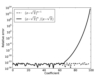
(a)

(b)

Figure 2.1: Accumulation of rounding error in the coefficients when the polynomial $p(x)$ is deflated by $(x-a)$, $a$ being a root.

Within the error bound of Theorem 2.1, there are two different mechanisms for large rounding errors. These two mechanisms are illustrated in Figure 2.1. Figure 2.1a shows the relative errors in the coefficients of $(x-\sqrt{2})^{99}$ computed in two ways. The first computation begins with $(x-\sqrt{2})^{100}$ and then divides by $x-\sqrt{2}$. In the second computation, $99$ factors $x-\sqrt{2}$ are multiplied. In the first computation, it is seen that the relative errors are initially small but begin to explode after the half way mark. In contrast, the relative errors remain small throughout in the second computation.

The error bound in Theorem 2.1 corresponds to the exact formula $c_{k}=-\sum_{j=0}^{k}b_{j}/a^{k+1-j}$. The relative error in $c_{k}$ will be large if some of the terms of this sum are much larger than $c_{k}$. In the binomial expansion, the coefficients at the edges are much smaller than the ones in the middle. Thus deflation, using the method of Theorem 2.1, leads to large errors once we get past the middle. This is the first mechanism for large rounding errors.

The Chebyshev polynomial $T_{n}(x)$ is defined as $\cos(n\arccos x)$ for $x\in[-1,1]$. All its $n$ roots are in the interval $[-1,1]$. Figure 2.1b shows the errors in the coefficients of $T_{n}(x)/(x-a)$, where $a$ is a root close to $0$ and when $a$ is a root close to $1$. The errors grow explosively for $a\approx 0$ ($k=53$ in the plot), but are quite mild when $a\approx 1$ ($k=3$ in the plot). Here too, as indicated by Theorem 2.1, there must be cancellations between the terms of $-\sum_{j=0}^{k}b_{j}/a^{k+1-j}$ for large relative errors. The cancellations can be particularly severe when $a$ is small. This is the second mechanism for large rounding errors.

One of the methods for computing spectral differentiation matrices [13, 14] suffers from an instability related to the second mechanism. This instability has been completely fixed [9], yet we explain exactly how it comes about. In the original formulation [13, 14], the connection to polynomials and root deflation is not transparent.

Equation (7) of [14], which is the heart of the algorithm in that paper, reads as follows:

$$\left(D_{p+1}\right)_{k,j}=\frac{p+1}{x_{k}-x_{j}}\left(\frac{c_{k}}{c_{j}}\left(D_{p}\right)_{k,k}-\left(D_{p}\right)_{k,j}\right).$$

Here $\left(D_{p}\right)_{k,j}$ denotes the coefficient at $x_{j}$ of the $p$-th derivative at $x_{k}$. The grid points $x_{0},x_{1},\ldots,x_{n}$ are assumed to be distinct. The $c_{i}$ are normalizing constants extraneous to the discussion here and will be ignored.

Let $l_{j}(x)$ denote the Lagrange cardinal function which is equal to $1$ at $x_{j}$ and $0$ at the other grid points. The coefficients of $u^{p}$ and $u^{p+1}$ in the polynomial $l_{j}(u+x_{k})$

$$\frac{\left(u+x_{k}-x_{1}\right)\left(u+x_{k}-x_{2}\right)\cdots\left(u+x_{k}-x_{n}\right)}{u+x_{k}-x_{j}},$$

multiplied by normalizing constants which we ignore, are equal to the $p$-th and $(p+1)$-st derivatives of the Lagrange cardinal function $l_{j}(x)$ evaluated at $x_{k}$, respectively (see [9]). Similarly, the coefficient of $u^{p+1}$ of $\prod_{i=1}^{n}\left(u+x_{k}-x_{i}\right)$, multiplied by a normalizing constant which we ignore, is equal to the $p$-th derivative of the Lagrange cardinal function $l_{k}(x)$ evaluated at $x_{k}$[9]. Finite difference weights are nothing but the coefficients of Lagrange cardinal functions, suitably normalized. It follows that equation (7) of [14] is using exactly the same recurrence as in Theorem 2.1 and is therefore susceptible to the instability exhibited above.

Root deflation is a part of polynomial root finding algorithms such as Jenkins-Traub [6]. In these applications, the equations (2.1) are solved for $c_{i}$ in the order $c_{n-1},c_{n-2},\ldots,c_{0}$. The bound in the following theorem is proved in much the same way as the bound in Theorem 2.1.

Theorem 2.2.

If the equations (2.1) are solved for $c_{i}$ in the order $c_{n-2},c_{n-1},\ldots,c_{0}$ (bottom to top in (2.1)), the error in the computed quantity $\hat{c}_{k}$ satisfies the bound

$$\big{|}\hat{c}_{k}-c_{k}\bigr{|}\leq|b_{k+1}|\gamma_{1}+|ab_{k+2}|\gamma_{3}+\cdots+|a|^{n-k-1}\gamma_{2n-2k+1}.$$

The computation in Theorem 2.2 corresponds to the formula $c_{k}=a^{n-k-1}+\sum_{j=k+1}^{n-1}b_{j}a^{j-k-1}$. This appears a safer method because it is not vulnerable to the second mechanism when $a\approx 0$, and if the coefficients are well-scaled we may assume that the roots $a$ are not too large. However, it is still vulnerable to the first mechanism. For example, if this algorithm is applied to deflate a factor of $\left(x-a\right)^{n}$, large errors in the coefficients will occur for powers lower than $x^{n/2}$.

In the computation of finite difference weights, both instability mechanism are avoided by the method of partial products [9]. In that method the operation of deflating a polynomial by a factor is not employed. Going by analogy, it is natural to make the suggestion that polynomial root finding algorithms that avoid root deflation may be more accurate for each individual root. The operation count may be higher, but the polynomial root finding problems are puny compared to the power of modern computers. Thus accuracy is of greater consequence.

2.2 Inversion of a quadratic

In a quadratic $ay^{2}+by+c$ with $ac\neq 0$, we may make the change of variables $x=sy$ and choose the scale factor $s$ to make the coefficients of $x^{2}$ and $x$ equal in magnitude. If the coefficient of $x^{2}$ is factored out we are left with a quadratic of the form $x^{2}+bx\pm 1$. The operations of factoring out the leading coefficient and rescaling the variable induce minimal relative error in the computed coefficients. Therefore as far as the accumulation of error in the coefficients of the inverse is concerned, we are left with only two cases:

$$\frac{1}{x^{2}+bx\pm 1}=\pm 1+c_{1}x+c_{2}x^{2}+\ldots$$

In the $-1$ case, we have $c_{1}=-b$, $c_{2}=bc_{1}-1$, and $c_{n+1}=bc_{n}+c_{n-1}$. It follows that $c_{i}$ has the opposite sign to $b$ if $i$ is odd and is negative if $i$ is even. There are no cancellations and all coefficients are computed with excellent relative accuracy. Both roots of the quadratic equation $x^{2}+bx-1=0$ are real.

The other case is with $+1$. In this case, we have

$$c_{1} = -b$$

$$c_{2} = b^{2}-1$$

$$c_{3} = -b^{3}+2b$$

$$\vdots$$

In general, $c_{n+1}=-bc_{n}-c_{n-1}$. Each $c_{n}$ is a polynomial in $b$: $c_{n}=F_{n}(b)$ where $F_{n}$ is a polynomial of degree $n$. If $\alpha$ and $\beta$ are the two distinct roots of $x^{2}+bx+1=0$ it follows that

$$c_{n}=F_{n}(b)=\frac{1}{\beta-\alpha}\left(\frac{1}{\beta^{n+1}}-\frac{1}{\alpha^{n+1}}\right).$$ (2.2)

To keep the discussion simple we omit the cases $b=\pm 2$ with repeated roots. The polynomials $F_{n}$ are a version of Fibonacci polynomials [5]. An easy induction argument using the recurrence $c_{n+1}=-bc_{n}-c_{n-1}$ proves that the polynomial $c_{2n}=F_{2n}(b)$ has only even degree terms and that the coefficients alternate in sign beginning with $b^{2n}$. Similarly, $c_{2n+1}=F_{2n+1}(b)$ has only odd degree terms and the coefficients alternate in sign beginning with $-b^{2n+1}$.

If we write $c_{n-1}=F_{n-1}(b)=\sum_{k=0}^{n-1}C_{n-1,k}b^{k}$, we may inductively assume that the computed quantity $\hat{c}_{n-1}$ is given by $\sum_{k=0}^{n-1}C_{n-1,k}b^{k}(1+\theta_{2n-2})$. Likewise, we may inductively assume that $\hat{c}_{n}=\sum_{k=0}^{n}C_{n,k}b^{k}(1+\theta_{2n})$. The recurrence $c_{n+1}=-bc_{n}-c_{n-1}$ implies that $C_{n+1,k}b^{k}=-\left(C_{n,k-1}b^{k-1}\right)b-C_{n-1,k}b^{k}$, where crucially $C_{n,k-1}$ and $C_{n-1,k}$ have the same sign, thanks to the pattern in the signs of the coefficients of $F_{n}(b)$ and $F_{n-1}(b)$. Therefore we may infer that $\hat{c}_{n+1}=\sum_{k=0}^{n+1}C_{n+1,k}b^{k}(1+\theta_{2n+2})$, completing the induction.

The error bound

$$\frac{|c_{n}-\hat{c}_{n}|}{|c_{n}|}\leq\frac{|F_{n}|\left(|b|\right)}{\Bigl{|}F_{n}(b)\bigr{|}}\gamma_{2n},$$

where $|F_{n}|$ is the polynomial with all coefficients of $F_{n}$ replaced by their absolute values, follows immediately. If we go back to formula (2.2) for $c_{n}$, we get a sense of when the relative errors in the computed coefficients may be large. If $|b|<2$, both roots $\alpha$ and $\beta$ of $x^{2}+bx+1$ are complex of magnitude $1$ and conjugates of each other. For certain values of $n$, the arguments of $\alpha^{n+1}$ and $\beta^{n+1}$ will differ very nearly by a multiple of $2\pi$ and formula (2.2) implies a cancellation making $F_{n}(b)$ much smaller in magnitude than $|F_{n}|\left(|b|\right)$. The corresponding coefficients $c_{n}$ will have large relative errors.

2.3 Connection to pseudozeros

Let $p=p_{0}+p_{1}z+p_{n-1}z^{n-1}+z^{n}$ be a monic polynomial and let $Z(p)=\{a_{1},a_{2},\dots,a_{n}\}$ be the set of roots of $p$. We assume $p_{0}\neq 0$. We shall connect the errors in computing the inverse series $q(z)=1/p(z)$ to the pseudozeros of $p(z)$. The analysis here is of conditioning not of rounding errors. We consider another monic polynomial $\hat{p}$ close to $p$ and bound the errors in $\hat{q}=1/\hat{p}$ using the pseudozero sets of $p$. The subscripted variable $p_{i}$ denotes the coefficient of $z^{i}$ in $p(z)$. Similarly $q_{i}$ denotes the coefficient of $z^{i}$ in $q(z)$.

Pseudozero sets have been defined using the infinity norm [7] or more general norms [11]. Here we define pseudozero sets using the maximum coefficient-wise relative error. Our definition is close to that of [7]. Let

$$e(\hat{p}):=\max_{i,p_{i}\neq 0}\frac{|p_{i}-\hat{p}_{i}|}{|p_{i}|}$$

be the maximum coefficient-wise error in $\hat{p}$ relative to $p$. The $\epsilon$-pseudozero set of $p$ in the complex plane is given by

$$Z_{\epsilon}(p):=\{z\in\mathbb{C}\;:\;z\in Z(\hat{p}),\;e(\hat{p})\leq\epsilon\}.$$

An argument in [7] (also see [11]) implies that

$$Z_{\epsilon}(p)=\left\{z\in\mathbb{C}\;:\;\frac{|p(z)|}{|p|(|z|)}\leq\epsilon\right\}$$

where $|p|$ is the polynomial with all coefficients of $p$ replaced by their absolute values.

Suppose $\hat{a}\in Z_{\epsilon}(p)$ and let $a\in Z(p)$, with $a=a_{i}$ for some $i$, be the root closest to $\hat{a}$. All the roots $a_{i}$ of $p(x)=0$ are assumed to be distinct, to avoid technicalities of no value for the discussion here. Then

$$|a-\hat{a}|^{n}\leq\prod_{i,p(a_{i})=0}|\hat{a}-a_{i}|=|p(\hat{a})|\leq\epsilon|p|(|\hat{a}|)$$

since $p$ is a monic polynomial. We have

$$|a-\hat{a}|\leq\sqrt[n]{\epsilon|p|(|\hat{a}|)},$$

but this bound on the error is highly pessimistic. This bound is reasonably good only if $|\hat{a}-a|\approx|\hat{a}-a_{i}|$ for every $i$, which is very seldom the case.

Condition numbers of polynomials roots [2, 11] may be used to derive better and less pessimistic bounds. If $a_{j}$ is a simple root of $p$ we may define

$$\kappa(a_{j},p):=\lim_{e(\hat{p})\to 0}\sup_{\hat{p}}\frac{|a_{j}-\hat{a}_{j}|}{e(\hat{p})}$$

where $\hat{a}_{j}$ is the root of $\hat{p}$ corresponding to $a_{j}$ and $e(\hat{p})$ is the maximum relative coefficient-wise distance of $\hat{p}$ from $p$ defined earlier. If $e(\hat{p})<\epsilon$ and $\epsilon\to 0$, we have,

$$\frac{p(\hat{a}_{j})}{p^{\prime}(a_{j})(\hat{a}_{j}-a_{j})}=\frac{(\hat{a}_{j}-a_{1})\cdots(\hat{a}_{j}-a_{j-1})(\hat{a}_{j}-a_{j+1})\cdots(\hat{a}_{j}-a_{n})}{(a_{j}-a_{1})\cdots(a_{j}-a_{j-1})(a_{j}-a_{j+1})\cdots(a_{j}-a_{n})}\to 1$$

implying $\hat{a}_{j}-a_{j}\approx p(\hat{a}_{j})/p^{\prime}(a_{j})$. Therefore, we have

$$\kappa(a_{j},p)=\lim_{\epsilon\to 0}\sup_{\hat{p},e(\hat{p})\leq\epsilon}\frac{|p(\hat{a}_{j})|/|p^{\prime}(a_{j})|}{e(\hat{p}_{j})}=\frac{|p|(|a_{j}|)}{|p^{\prime}(a_{j})|}$$

noting that the inequality $|p(\hat{a})|\leq\epsilon|p|(|\hat{a}|)$ is sharp for some polynomial $\hat{p}$ with $e(\hat{p})=\epsilon$ (see [7]).

If $p$ has only distinct roots as assumed, we have

$$q(z)=\frac{\text{Res}(q,a_{1})}{(z-a_{1})}+\cdots+\frac{\text{Res}(q,a_{n})}{(z-a_{n})}$$

where the residue of $q$ at one of its simple poles $a_{j}$ is given by $\text{Res}(q,a_{j})=1/[(a_{j}-a_{1})\cdots(a_{j}-a_{j-1})(a_{j}-a_{j+1})(a_{j}-a_{n})]$. We may expand $q$ as

$$q(z)=\sum_{j=1}^{n}\text{Res}(q,a_{j})\left(\frac{-1}{a_{j}}\right)\sum_{k=0}^{\infty}\left(\frac{z}{a_{j}}\right)^{k}=\sum_{k=0}^{\infty}\left(\sum_{j=1}^{n}\frac{-\text{Res}(q,a_{j})}{a_{j}^{k+1}}\right)z^{k}.$$

Let $\hat{q}=1/\hat{p}$, where $e(\hat{p})\leq\epsilon$, and let $Z(\hat{p})=\{\hat{a}_{1},\dots,\hat{a}_{n}\}$ with $\hat{a}_{i}$ corresponding to $a_{i}$, with $\epsilon$ assumed small enough that the correspondence may be set up. The error in the coefficient of $z^{k}$ is

$$(q-\hat{q})_{k}=\sum_{j=1}^{n}\left(\frac{\text{Res}(\hat{q},\hat{a}_{j})}{\hat{a}_{j}^{k+1}}-\frac{\text{Res}(q,a_{j})}{a_{j}^{k+1}}\right).$$

A perturbative calculation of error, assuming $\epsilon$ so small that $\Delta a_{i}=\hat{a}_{i}-a_{i}$ satisfies $|\Delta a_{i}|\ll|a_{j}-a_{k}|$ for any $i,j,k$, follows. The perturbative calculation is based on

$$\text{Res}(\hat{q},\hat{a}_{j})=\text{Res}(q,a_{j})\left(1-\sum_{i\neq j}\frac{\Delta a_{j}-\Delta a_{i}}{a_{j}-a_{i}}\right)+\mathcal{O}(\Delta a^{2})$$

and

$$\frac{1}{\hat{a}_{j}^{k+1}}=\frac{1}{a_{j}^{k+1}+ka_{j}^{k}\Delta a_{j}+\mathcal{O}(\Delta a_{j}^{2})}=\frac{1}{a_{j}^{k+1}}-\frac{\left(k+1\right)a_{j}^{k}\Delta a_{j}}{a_{j}^{2\left(k+1\right)}}+\mathcal{O}(\Delta a_{j}^{2}).$$

These complete the first order perturbative calculation by implying

$$(q-\hat{q})_{k}=-\sum_{j=1}^{n}\frac{\text{Res}(q,a_{j})}{a_{j}^{k+1}}\left(\frac{(k+1)\Delta a_{j}}{a_{j}}+\sum_{i\neq j}\frac{\Delta a_{j}-\Delta a_{i}}{a_{j}-a_{i}}+\mathcal{O}(\Delta a^{2})\right).$$ (2.3)

Turning to condition number of roots of $p(z)=0$, we get the asymptotic bound

$$|(q-\hat{q})_{k}|\lesssim\epsilon\sum_{j=1}^{n}\left|\frac{\text{Res}(q,a_{j})}{a_{j}^{k+1}}\right|\left(\frac{(k+1)\kappa(a_{j},p)}{|a_{j}|}+\sum_{i\neq j}\frac{\kappa(a_{i},p)+\kappa(a_{j,}p)}{|a_{j}-a_{i}|}\right).$$ (2.4)

This bound suggests that the error in the $k$-th coefficient is dominated by the root closest to $0$ in the limit $k\rightarrow\infty$. In the transient phase, it suggests that some of the exterior roots may dominate the error if they are sufficiently ill-conditioned. The latter suggestion is not well-founded for a reason that will be presently explained.

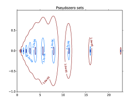
(a)

(b)

(c)

(d)

Figure 2.2: Pseudozero sets and plots of relative error vs. coefficient for a well-conditioned polynomial ((a) and (b)) and an ill-conditioned one ((c) and (d)), both of degree $13$. The bound (2.4) bounds absolute errors. It is converted to a bound on relative errors in the plots.

Figure 2.2 compares the bound (2.4) (dashed line) to actual errors (solid line) for two examples. The first example is $\prod_{i=-3}^{9}\left(x-2^{i/2}\right)$, implying well-conditioned roots, and the second example is $\prod_{i=1}^{13}(x-i\sqrt{2})$, implying ill-conditioned roots. Both examples are based on [16]. In both examples, the bound (2.4) suggests transient errors at the beginning which never materialize. The bound is highly pessimistic for the ill-conditioned example.

Part of the problem with the bound (2.4) is that the condition numbers $\kappa(a_{j},p)$ can overestimate the perturbation to the roots. But a more serious problem is that the errors $\Delta a_{i}$ in the first order error estimate (2.3) are highly correlated and this correlation is lost when they are bounded using $\kappa(a_{j},p)$. Since $p$ and $\hat{p}$ are both monic polynomials, the negative sums of their roots must equal $p_{n-1}$ and $\hat{p}_{n-1}$, respectively. Therefore no matter how large each perturbation $\Delta a_{i}$ may be, their sum $\sum\Delta a_{i}$ must be of the order of machine precision, implying correlation between the errors.

Such correlation between the errors $\Delta a_{i}$ is lost in the asymptotic bound $|\Delta a_{i}|\lesssim\kappa(a_{i},p)$. Whether the pseudozero plots contain information about correlations in the errors is unknown.

It is reasonable to expect a numerically stable algorithm for finding roots to reproduce symmetric functions, such as the sum of all the roots or the product of all the roots, accurately. However the algorithms in current use progress from root to root, deflating the polynomial every time a root is found. Perhaps for that reason they do not seem to have this property. In particular algorithms that deflate using the method of Theorem 2.2 will reproduce the sum of the roots with accuracy but not the product of the roots.

3 Error bounds and numerical stability

The analysis given in this section uses techniques pioneered by Wilkinson [15] and refined by Higham [3, 4]. The application of the techniques is specialized to the inversion of power series. Near the end of the section, we discuss the work of Stewart [10] when comparing the errors that are realized with the error bounds.

3.1 Rounding error analysis

To invert a power series as in

$$\frac{1}{1+b_{1}x+b_{2}x^{2}+\cdots}=1+c_{1}x+c_{2}x^{2}+\cdots$$

the coefficients $c_{i}$ may be computed using

$$c_{1} = -b_{1}$$

$$c_{2} = -b_{2}-c_{1}b_{1}$$

$$\vdots$$

$$c_{k} = -b_{k}-c_{1}b_{k-1}-\cdots-c_{k-1}b_{1}$$ (3.1)

The subtractions here are assumed to be left to right associative, unlike Wilkinson’s analysis of triangular back-substitution [15] which assumes the opposite. Left to right associativity has the advantage of preserving the Toeplitz structure of the matrices that arise in error bounds.

If we define $C_{n}$ and $T_{n}$ as

$$C_{n}=\left(\begin{array}[]{c}1\\ c_{1}\\ c_{2}\\ \vdots\\ c_{n}\end{array}\right),T_{n=}\left(\begin{array}[]{ccccc}1\\ b_{1}&1\\ b_{2}&b_{1}&1\\ \vdots&\vdots&\vdots&\ddots\\ b_{n}&b_{n-1}&b_{n-2}&\ldots&1\end{array}\right)\,\,\text{then}\,\,T_{n}^{-1}=\left(\begin{array}[]{ccccc}1\\ c_{1}&1\\ c_{2}&c_{1}&1\\ \vdots&\vdots&\vdots&\ddots\\ c_{n}&c_{n-1}&c_{n-2}&\ldots&1\end{array}\right).$$ (3.2)

Here $T_{n}^{-1}$ is, like $T_{n}$, a Toeplitz matrix. In addition, we have $T_{n}C_{n}={\bf e}_{1}$ where ${\bf e}_{1}$ is the vector whose first component is $1$ and all others are $0$. In the recursion (3.1) for computing $c_{k}$, the last $c_{k-1}b_{1}$ term participates in only two arithmetic operations, namely, the multiplication of $c_{k-1}$ and $b_{1}$ and the subtraction of that product. Earlier terms participate in more subtractions and the second term, which is $-c_{1}b_{k-1}$, participates in $k$ subtractions. If the computed quantity is denoted $\hat{c}_{k}$, we may write

$$\hat{c}_{k}=-b_{k}\left(1+\theta_{k+1}\right)-\hat{c}_{1}b_{k-1}\left(1+\theta_{k}\right)-\cdots-\hat{c}_{k-1}b_{1}\left(1+\theta_{2}\right).$$

In other words, if $\hat{C}_{n}$ is the vector made up of $\hat{c}_{1},\ldots,\hat{c}_{n}$, we have $\left(T_{n}+\Delta T_{n}\right)\hat{C}_{n}={\bf e}_{1}$ with $\bigl{|}\Delta T_{n}\bigr{|}\leq E_{n}$, where

$$E_{n}=\left(\begin{array}[]{ccccc}0\\ \gamma_{2}|b_{1}|&0\\ \gamma_{3}|b_{2}|&\gamma_{2}|b_{1}|&0\\ \vdots&\vdots&\vdots&\ddots\\ \gamma_{n+1}|b_{n}|&\gamma_{n}|b_{n-1}|&&\ldots&0\end{array}\right).$$ (3.3)

The identity

$$\left(\hat{C}_{n}-C_{n}\right)=-T_{n}^{-1}\Delta T_{n}\left(\hat{C}_{n}-C_{n}\right)-T_{n}^{-1}\Delta T_{n}C_{n}$$ (3.4)

is the basis of the error bounds.

We may take norms of either side of (3.4) and get

$$|\hat{c}_{n}-c_{n}|\leq\bigl{|}\bigl{|}C_{n}-\hat{C}_{n}\bigr{|}\bigr{|}\leq\frac{\Bigl{|}\Bigl{|}|T_{n}^{-1}|\>E_{n}\>|C_{n}|\Bigr{|}\Bigr{|}_{\infty}}{1-\Bigl{|}\Bigl{|}|T_{n}^{-1}|\>E_{n}\Bigr{|}\Bigr{|}_{\infty}}.$$ (3.5)

However, this bound is very poor. The coefficients of power series are typically scaled badly, with terms increasing or decreasing at a rapid rate. Norm-wise bounds are not of much use.

To get a component-wise bound, we go back to (3.4) and take absolute values of both sides.

$$\left|\hat{C}_{n}-C_{n}\right| \leq \left|T_{n}^{-1}\right|\,E_{n}\,\left|\hat{C}_{n}-C_{n}\right|+\left|T_{n}^{-1}C_{n}\right|\,E$$

$$\left(I-\left|T_{n}^{-1}\right|\,E_{n}\right)\left|\hat{C}_{n}-C_{n}\right| \leq \left|T_{n}^{-1}C_{n}\right|\,E_{n}.$$

Noting that the matrix $\left(I-\left|T_{n}^{-1}\right|\,E_{n}\right)$ is lower triangular with a non-negative inverse, we have the following theorem.

Theorem 3.1.

If a power series is inverted using the recurrence (3.1) and left to right associativity, we have the error bound

$$\left|\hat{C}_{n}-C_{n}\right|\leq\left(I-\left|T_{n}^{-1}\right|\,E_{n}\right)^{-1}\left|T_{n}^{-1}C_{n}\right|\,E_{n}.$$ (3.6)

3.2 Condition analysis and numerical stability

If $p$ is a power series, $|p|$ denotes the power series with coefficients replaced by their absolute values. Let $p$ and $q$ be power series with constant terms equal to $1$ and

$$pq=1.$$

If $p$ is perturbed to $p+\Delta p$, where the constant term of $\Delta p$ is $0$, suppose that $q$ gets perturbed to $q+\Delta q$. We have

$$(p+\Delta p)(q+\Delta q)=1.$$

It follows that

$$p\Delta q = -q\Delta p-\Delta p\Delta q$$

$$\Delta q = -q^{2}\Delta p-q\Delta p\Delta q$$

$$|\Delta q| \leq |q^{2}\Delta p|+|q\Delta p|\,|\Delta q|$$

$$\left(1-|q|\Delta p|\right)|\Delta q| \leq |q^{2}\Delta p|$$

All the coefficients of the power series $1/(1-|q\Delta p|)$ are positive. Therefore we may multiply by that power series to get the bound

$$|\Delta q|\leq\frac{|q^{2}\Delta p|}{1-|q\Delta p|}\leq\frac{|q^{2}|\,|\Delta p|}{1-|q|\,|\Delta p|}.$$ (3.7)

We may take $|\Delta p$| to be

$$\sum_{j=1}^{\infty}u|p_{j}|x^{j},$$ (3.8)

where $u$ is the unit round-off, to obtain a bound on each entry of $q$ using (3.7). Here it is significant that the constant term of $\Delta p$ is zero. The conditioning bound (3.7), with $|\Delta p|$ given by (3.8), is sharp up to first order for each coefficient of $\Delta q$ with a suitable choice of the signs of the coefficients of $|\Delta p|$.

Armed with this conditioning bound, we may consider the numerical stability of the inversion of power series using the recurrence (3.1). Theorem 3.6 states that

$$\left|\hat{C}_{n}-C_{n}\right|\leq\left(I-\left|T_{n}^{-1}\right|\,E_{n}\right)^{-1}\left|T_{n}^{-1}C_{n}\right|\,E_{n}.$$

From the definitions of $C_{n}$ and $T_{n}^{-1}$ in (3.2) as well as that of $E_{n}$ in (3.3), we get

$$\bigl{|}C_{n}-\hat{C}_{n}\bigr{|}\leq\frac{2(n+1)|q^{2}|\,|\Delta p|}{1-2(n+1)|q||\Delta p|}.$$

Here we have used $\gamma_{k}<\gamma_{n+1}$ for $k\leq n$ and $\gamma_{n+1}\leq 2(n+1)u$, which assumes $(n+1)u<1/2$. This bound differs from the conditioning bound (3.7) for each coefficient by only a polynomial factor in $n$. Therefore inversion of power series using back substitution is numerically stable.

3.3 Numerical examples

(a)

(b)

(c)

(d)

Figure 3.1: Rounding error bounds and actual rounding errors for four examples. The bound of Theorem 3.6 is on absolute error. That bound is converted to a bound on relative error for bound 1 in each of the plots. Likewise, the bound of (3.7), with $|\Delta p|$ given by (3.8), is converted to bound 2. Each plot graphs relative error in the $n$-th coefficient vs. $n$.

Figure (3.1) shows that the bounds of Section 3.1 and 3.2 do quite well on four different examples. The bounds themselves were computed using extended precision of $100$ digits. The actual relative error was computed by comparing the double precision answers with extended precision answers. For inversion of cosine, $1/\cos x$ in Figure (3.1)b, the odd terms were ignored. It may be noted that the inverse cosine series is one of the ways of defining Euler numbers. In the “randn” series, each $b_{i}$ in $p(x)=1+\sum_{i=1}^{\infty}b_{i}x^{i}$ is an independent standard normal variable.

Error bounds for inversion of triangular matrices are similar to that of Theorem 3.6. However, they often overestimate the error greatly [15]. In particular, for many triangular matrices the relative error in the inverse appears independent of the condition number. Here we discuss the work of Stewart [10] and connect it to the inversion of power series.

Consider the upper triangular matrix

$$\left(\begin{array}[]{cc}R&r\\ 0&\delta\end{array}\right).$$ (3.9)

If $\sigma$ is its smallest singular value, suppose $\sigma\geq\beta\delta$, where $\beta\in[0,1]$ must hold. If $\beta$ is not too tiny, the matrix is rank-revealing in the sense of Stewart. The last row of this matrix may be rescaled to get

$$\left(\begin{array}[]{cc}R&r\\ 0&1\end{array}\right),$$

whose least singular value is denoted $\hat{\rho}$. If the least singular value of $R$ is $\rho$, Stewart [10] has proved that

$$\hat{\rho}\geq\frac{\beta\rho}{\sqrt{\beta^{2}+\rho^{2}}}.$$

This bound may be interpreted as follows. If the matrix (3.9) is rank-revealing with a $\beta$ that is not too tiny, any significant fall in the least singular value when we move from $R$ to that matrix must be due to the smallness of $\delta$. The smallness of $\delta$ can be easily eliminated by rescaling the last row to get a matrix whose condition number $\hat{\rho}$ is only moderately smaller than $\rho$ the condition number of $R$. On the other hand, if the best possible $\beta$ is quite tiny, it may mean that the ill-conditioning of the matrix (3.9) is hidden within the correlations between rows in a way that may not be eliminated so easily. If each one of the principal submatrices of a matrix is rank revealing, any ill-conditioning is almost entirely removed by rescaling rows explaining Wilkinson’s observation.

Many triangular matrices are not rank-revealing. For example, random triangular matrices are not rank-revealing with probability $1$ as proved in [12]. However, Stewart [10] argues intuitively that the triangular matrices that arise in Gaussian elimination and QR factorization are likely to be rank revealing. His argument is that if a matrix is rank deficient, Gaussian elimination and QR will break down with a $0$ on the diagonal. If it is nearly rank deficient, continuity suggests that a very small entry must appear on the diagonal indicating its rank deficiency. Pivoting makes either factorization more apt to be rank revealing.

To connect Stewart’s analysis to power series, we shall assume that $p(x)=1+\sum b_{i}x^{i}$ has a radius of convergence $R$ equal to $1$. Any finite radius of convergence can be turned into $1$ by the change of variables $x\leftarrow x/R$. Assuming $R=1$, the matrix $T_{n}$ of (3.2) is rank-revealing if and only if its least singular value is $\mathcal{O}(1)$. The least singular value of $T_{n}$ is $\mathcal{O}\left(1\right)$ if and only if the greatest singular value of $T_{n}^{-1}$is $\mathcal{O}(1)$, which is true if and only if the entries $c_{i}$ of $T_{n}^{-1}$ in (3.2) are $\mathcal{O}(1)$. Since $c_{i}$ are the coefficients of the power series of $1/p(x)$, we have that $T_{n}$ is rank revealing in the sense of Stewart if and only if the radius of convergence of $1/p(x)$ is $1$ or greater.

If the equation $p(z)=0$ has a solution with $|z|<1$ in the complex plane, the matrix $T_{n}$ will not be rank-revealing. The example of Figure 3.1d, $p(z)=1+\log(1+z)$ has a zero at $z=1-1/e$ and the corresponding matrix $T_{n}$ is not rank-revealing. If in fact the radius of converge of $p(z)$ is $1$ and there is no zero with $|z|<1$, the matrix $T_{n}$ will be rank-revealing but its condition number will be $\mathcal{O}(1)$. Within the scope of the analysis given by Stewart, the situation where the actual relative errors are much smaller than the conditioning bound appears unlikely. The good agreement between the bounds and the actual errors in Figure 3.1 is the rule rather than the exception.

4 Conclusions

In this article, we have considered the inversion of power series with particular attention to the special case of inverting polynomials. Essential background is provided by the classic work of Wilkinson [15] on inversion of triangular systems.

We found and explicated a subtle numerical instability that arises when factors corresponding to known roots are deflated from polynomials. This instability has occurred in the computation of spectral differentiation matrices. The suggestion that polynomial root finding algorithms such as Jenkins-Traub may be more accurate without the deflation step merits further investigation.

The rounding error analysis and the condition analysis of power series inversion imply numerical stability. In addition, the error bounds that result from the analysis are not unduly pessimistic, as happens for certain other triangular systems.

5 Acknowledgements

This research was partially supported by NSF grants DMS-1115277 and SCREMS-1026317.

References

- [1] J.C. Butcher, R.M. Corless, L. Gonzalez-Vega, and A. Shakoori. Polynomial algebra for Birkhoff interpolants. Numerical Algorithms, 56:319–347, 2011.
- [2] W. Gautschi. Questions of numerical condition related to polynomials. In G.H. Golub, editor, Studies in Numerical Analysis, volume 24 of MAA Studies in Mathematics, pages 140–177. MAA, 1984.
- [3] N.J. Higham. The accuracy of solutions to triangular systems. SIAM J. Numer. Anal., 26(5):1252–1265, 1989.
- [4] N.J. Higham. Accuracy and Stability of Numerical Algorithms. SIAM, Philadelphia, 2nd edition, 2002.
- [5] V.E. Hoggatt Jr. and M Bicknell. Roots of Fibonacci polynomials. Fibonacci Quarterly, 11(3):271–274, 1973.
- [6] M.A. Jenkins and J.F. Traub. A three stage variable-shift iteration for polynomial zeros and its relation to generalized Rayleigh iteration. Numer. Math., 14:252–263, 1970.
- [7] R.G. Mosier. Root neighborhoods of a polynomial. Mathematics of Computation, 47(175):265–273, 1986.
- [8] B. Sadiq and D. Viswanath. Barycentric Hermite interpolation. SIAM J. Sci. Comput., 35(3):A1254–A1270, 2013.
- [9] B. Sadiq and D. Viswanath. Finite difference weights, spectral differentiation, and superconvergence. Mathematics of Computation, 83:2403–2427, 2014.
- [10] G.W. Stewart. The triangular matrices of Gaussian elimination and related decomposition. IMA Journal of Numerical Analysis, 17:7–16, 1997.
- [11] K.-C. Toh and L.N. Trefethen. Pseudozeros of polynomials and pseudospectra of companion matrices. Numer. Math., 68:403–425, 1994.
- [12] D. Viswanath and L.N. Trefethen. Condition numbers of random triangular matrices. SIAM Journal on Matrix Analysis and Applications, 19:564–581, 1998.
- [13] J.A.C. Weideman and S.C. Reddy. A MATLAB differentiation matrix suite. ACM Transactions on Mathematical Software, 26(4):465–519, 2000.
- [14] B.D. Welfert. Generation of pseudospectral differentiation matrices I. SIAM Journal on Numerical Analysis, 34(4):1640–1657, 1997.
- [15] J.H. Wilkinson. Error analysis of direct methods of matrix inversion. J. Assoc. Comput. Mach., 8:281–330, 1961.
- [16] J.H. Wilkinson. The perfidious polynomial. In G.H. Golub, editor, Studies in Numerical Analysis, volume 24 of MAA Studies in Mathematics, pages 1–28. MAA, 1984.