Fast and Flexible Geometric Method For Enhancing MC Sampling of Compact Configurations For Protein Docking Problem

Abstract

EASAL (Efficient Atlasing and Sampling of Assembly Landscapes) is a geometric method for sampling and computing integrals over the potential energy landscape of small molecular assemblies. EASAL’s efficiency arises from the fact that small assembly landscapes permit the use of so-called Cayley (inter-atomic distance based) parameters for geometric representation and sampling of the assembly configuration space regions; this results in their isolation, convexification, customized sampling and systematic traversal using a comprehensive topological roadmap.

We define custom-designed measurements to investigate and compare various sampling characteristics of EASAL and the traditional Monte Carlo (MC) sampling, including (i) sampling speed, (ii) efficiency and accuracy of uniform grid coverage, (iii) accuracy of weighted coverage at covering low energy regions, (iv) ability to localize sampling to macrostates, and (v) flexibility in sampling distributions.

In particular, we compare the sampling characteristics of EASAL and MC in sampling the assembly landscape of 2 trans-membrane helices, with short-range pair-potentials. We demonstrate that EASAL provides a reasonable coverage of crucial but narrow regions of the energy landscape of low effective dimension, with much fewer samples and computational resources than MC sampling. Promising avenues for combining the complementary advantages of the two methods are discussed.

1 Introduction

To overcome the problem of incomplete sampling of relevant phase space when modeling protein assembly, in this paper, we use the geometric method EASAL (Efficient Atlasing of Assembly Landscapes)[1, 2, 3, 4]. In addition, we define custom-designed measurements to investigate and compare various sampling characteristics of EASAL and the traditional Monte Carlo (MC) sampling, including (i) sampling speed, (ii) efficiency and accuracy of uniform grid coverage, (iii) accuracy of weighted coverage at covering low energy regions, (iv) ability to localize sampling to macrostates, and (v) flexibility in sampling distributions.

In particular, we sample the energy landscape of two transmembrane helices assembling via short-range pair-potentials demonstrate that EASAL provides a reasonable coverage of crucial but narrow regions of the energy landscape of low effective dimension, with much fewer samples and computational resources than MC sampling. Promising avenues for combining the complementary advantages of the two methods are discussed.

EASAL partitions the energy landscape of transmembrane helices into nearly equipotential energy regions called active constraint regions or macrostates and organizes them into a query-able structure called the atlas. Each macrostate is a maximal, contiguous, nearly-equipotential-energy conformational region. In addition, EASAL uses the novel Cayley parameters, which are a distance-based internal coordinate representation of assembly configurations, to represent active constraint regions, yielding convex Cayley regions, a feature unique to assembly energy landscapes (as opposed to folding landscapes). Convexity of the Cayley regions improves sampling efficiency since sampling stays within the macrostates without having to explicitly enforce constraints. Convexity also avoids gradient descent and discarded and repeated samples which are common in other methods.

The EASAL methodology can quickly, without relying heavily on sampling, generate (1) a query-able atlas of local potential energy minima, their basin structure, and energy barriers between neighboring basins; (2) paths between a specified pair of basins, each path being a sequence of conformational regions or macrostates below a desired energy threshold; and (3) approximations of relative path lengths, basin volumes (configurational entropy), and path probabilities.

The theory and algorithms behind EASAL, including results for atlas generation decoupled from sampling, paths between basins, and approximate volume computation with minimal sampling appear in the papers[1, 2, 3] and are sketched in Section 2. Preliminary extensions of EASAL beyond dimer assemblies and viability of using EASAL for atlasing a wide variety of assembly systems including clusters of up to 24 assembling spherical particles is demonstrated in the paper[2]. The software implementation of EASAL (architecture and functionalities) is reported in [4]. The software has recently been employed to predict crucial inter-monomeric interface interactions for viral capsid assembly [5, 6].

In contrast, the primary focus of this paper is to illustrate sampling related features of EASAL through a variety of custom-designed measurements. This is important for EASAL’s performance in tasks that call for exact sampling, such as exact computation of basin volumes, path lengths and path probabilities. Specifically, we compare the performance of EASAL and MC with respect to the following sampling characteristics.

1. Speed: EASAL’s use of convexifying Cayley parameters allows it to avoid gradient descent which is used in MC to enforce constraints. In addition, it also reduces the number discarded samples, leading to high sampling speed. Results comparing the sampling speed of EASAL and MC are illustrated in Section 3.3.

2. Accuracy of uniform coverage: To measure the accuracy of coverage, we need to normalize the accuracy by the number of samples. In this paper this is measured by the $\varepsilon$-coverage (defined in Section 3.2). Results comparing the $\varepsilon$-coverage of MC and EASAL are illustrated in Section 3.3.

3. Efficiency of uniform coverage: When the goal of sampling is the coverage of the energy landscape, an efficient sampling algorithm should put as few points as possible in an $\varepsilon$-region, thereby reducing the number of repeated samples. Results comparing the efficiency of uniform coverage in EASAL and MC are illustrated in Section 3.3.

4. Accuracy of weighted coverage of lower energy regions: Certain applications may want lower energy regions to be sampled more densely, compared to higher energy regions. To compare the accuracy of sampling in such scenarios, we use the MultiGrid (defined in Section 3.1.4) as the reference grid for comparison. Results comparing MC and EASAL in terms of weighted coverage of lower dimensional regions are illustrated in Section 3.4.

5. Localized sampling of individual active constraint regions (macrostates): EASAL’s partitioning of the Energy landscape into active constraint regions and its use of convexifying Cayley parameters to represent these regions, allows it to localize sampling to individual active constraint regions or macrostates, of varying dimensions. EASAL can sample individual 5D, 4D, 3D, and 2D (with 1, 2, 3, and 4 active constraints respectively) regions of the energy landscape very fast, whereas MC has to sample the entire region to be able to locate these. Section 3.5 demonstrates EASAL’s flexibility at localized sampling of individual active constraint regions.

6. Flexibility of sampling distribution: EASAL’s sampling flexibility permits a variety of sampling distributions, from uniform Cayley parameter sampling, which is skewed towards lower energy regions, to uniform Cartesian sampling, which is essential for accurate computation of configurational entropy and other integrals. This is illustrated in Section 2.5, and for all the above sampling attributes, we compare MC with all the different variants of EASAL.

1.1 Motivation and Related Work

The problem of protein-protein assembly is an area of active research and development [7, 8, 9, 10, 11, 12, 13, 14]. Currently the most successful approach to docking two proteins together uses a direct exhaustive search of the whole configurational space. It is usually performed in the inverse space for translational moves on a cubic grid (using fast Fourier transforms (FFT)) [15]. The FFT algorithm makes the translation search very efficient, but it has to be repeated for all orientations of a molecule being docked resulting in thousands of FFT operations, each comprising millions of translations. The majority of the available software for molecular docking can only deal with two proteins (a dimer).

Several docking procedures are based on shape recognition and image segmentation techniques from Computer Vision [16]. The PatchDock algorithm [17] starts with a smooth representation of the molecular surface as a set of discrete points, but the set is restricted to critical points (convex caps, toroidal belts and concave pits), and the normal vectors at these points. A geometric hashing algorithm performs a very fast matching of the caps and pits with opposing normal directions on two surfaces, and collects all the rigid-body solutions that are geometrically acceptable after rejecting volume overlaps. Other geometric criteria can easily be incorporated in the procedure, for instance molecular symmetry in SymmDock [17], which allows building models of oligomeric proteins with up to twenty subunits. Unlike the goals of these methods, which is finding site-specific docking, the goal of EASAL and MC is sampling the entire configuration space of the assembly landscape.

A third class of methods, including Monte Carlo (MC) simulations and molecular dynamics (MD) are more prevalent in the study of protein folding and protein assembly than the other two. Both these techniques sample the system’s configuration space with probabilities corresponding to the Boltzmann distribution. Theoretically, such simulations can produce a probability density function for the whole phase space of the system. Absolute free energy and relative probabilities of various states in the phase space can then be estimated.

However, in practice, systems of interest are rarely ergodic, in the sense that their energy landscapes consist of an unknown number of energy minima separated by large energy barriers. Moreover, in tightly packed molecular systems, the majority of the phase space has high energy and low probability. In such conditions, most sampling procedures have a tendency to over sample local basins of the energy function, and have difficulty crossing over energy barriers. This results in uncertainty in both, i) relative probabilities of visited states, as well as ii) whether the range of low energy configurations visited during simulations is ever complete. Despite recent progress all currently existing methods of protein assembly are extremely computationally expensive.

In contrast to the more general applicability of MC and MD, the EASAL methodology applies only to assembly. However, it leverages geometric features unique to assembly (Cayley convexification, discussed in detail in Section 2.4) which gives it critical advantages when sampling assembly landscapes. In addition, the EASAL methodology comes with rigorously provable efficiency, accuracy, and tradeoff guarantees.

Organization: The rest of the paper is organized as follows. Section 2 briefly describes the EASAL methodology, highlighting its salient features and different sampling distributions. Section 3 compares the performance of EASAL and MC at sampling the potential energy landscape of the two assembling transmembrane helices. Section 4 discusses potential avenues to leverage the complementary strengths of both the methods. Section 5 gives conclusions and avenues for future work.

2 Materials and Methods

EASAL (Efficient Atlasing and Search of Assembly Landscapes) is a novel geometric methodology for analyzing free-energy and kinetics of assembly driven by short-range pair-potentials in an implicit solvent. The key concept of the new methodology is the atlas, which is a partition of the assembly landscape into nearly equipotential energy regions called active constraint regions or macrostates. The atlas is organized as a refinable, and query-able roadmap, which gives neighborhood relationships between active constraint regions. The active constraint regions have unique labels, which are graphs of active geometric constraints called active constraint graphs. The constraints are the pairwise Lennard-Jones potentials which drive assembly, along with sterics. Atom pairs (one from each transmembrane helix) are said to be an active constraint when the distance between their centers are in the Lennard-Jones’s well. The active constraint graphs are analyzed using geometric rigidity techniques, whereby the energy level of the active constraint region becomes a proxy for its dimension.

The EASAL methodology produces: (1) a query-able atlas of local potential energy minima, their basin structure, and energy barriers; and (2) approximations of basin volumes (configurational entropy). Leveraging its rigorous geometric underpinnings, EASAL can generate the topological roadmap of the energy landscape without relying heavily on sampling [2]. In addition, EASAL provides provable guarantees for tradeoffs between efficiency and accuracy.

The input to EASAL is an assembly system consisting of the following

1. A collection of $k$ rigid molecular components, each with at most $n$ atoms in them. The rigid molecular components are specified as the positions of atom-centers and atom radii, in a local coordinate system.

2. Pairwise component of the potential energy function, specified using Lennard-Jones potential energy terms (subsuming Hard-Sphere potential). The pairwise Lennard-Jones term for a pair of atoms, $i$ and $j$, one from each rigid molecular component, is given as a function of the distance $d_{i,j}$ between the centers of $i$ and $j$. The atom-center could, in some cases, be the representation for the average position of a collection of atoms in a residue.

3. A non-pairwise component of the potential energy function in the form of global potential energy terms that capture other factors including the implicit solvent (water or lipid bilayer membrane) effect [18, 19, 20]. These are specified as a function of the entire assembly configuration.

4. An optional set of constraints of interest, specified as a set of atom pairs, one from each rigid molecular component. When specified, only those configurations, which contain active constraints from the specified pairs of atoms are sampled.

5. The desired level of refinement of sampling is specified as the sampling step size $t$.

To sample the configuration space of an assembly system with input as described above, EASAL employs several key strategies including geometrization, stratification, recursive exploration of lower dimensional regions, and Cayley convexification. Each of these is described next.

2.1 Geometrization

The input Lennard-Jones pair potentials are geometrized, into distance constraints. For the inter-atomic short-range Lennard-Jones potential energy, the distance between the centers of atoms, are discretized into 3 main regions, large distances at which Lennard-Jones potentials are no longer relevant, short distances where inter-atomic repulsion kicks in and the interval between the two known as the Lennard-Jones’ well.

2.2 Stratification

EASAL partitions the energy landscape of the assembling transmembrane helices into active constraint regions. The active constraint regions are organized as a roadmap that captures their boundary relationships. In particular, the active constraint graph of a region is a subgraph of the active constraint graph of its children boundary regions. The children of a given region are 1 lower dimensional regions obtained when one additional constraint becomes active.

Configurations with more active constraints have lower potential energy and the lowest potential energy is attained at the bottoms of the potential energy basins. This leads to a dimensional stratification of the active constraint regions called a Thom-Whitney Stratification [21]. Intuitively, the active constraint regions are put in strata, one for each dimension and each stratum consists of active constraint regions of the same effective dimension. Figure 1 shows a screenshot from the EASAL software, depicting an atlas.

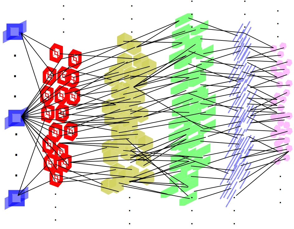
Figure 1: A portion of the stratified roadmap for the input molecules shown at the bottom right. The Active constraints regions of various dimensions are shown in different colors, 5D (blue), 4D (red), 3D (yellow), 2D (green), 1D (purple), 0D (pink). Edges indicate containment in a parent region one dimension higher. See Section 2.2.

2.3 Recursive exploration of lower dimensional active constraint regions

EASAL uses a recursive method that starts exploration from the interiors of higher dimensional regions and searches for the presence of boundary regions of exactly one lesser dimension (with exactly one extra active constraint). Searching for boundaries one dimension less at every stage, has a higher chance of success than looking for the lowest dimensional active constraint regions directly.

When a new child region is discovered, all its higher dimensional ancestor regions are immediately discovered since they correspond to active constraint regions with a subset of the active constraints. So, even if a small (hard-to-find) region is missed at some stage (due to the sampling step size being too large), if any of its descendants are found at a later stage, say via a larger (easy-to-find) sibling, the originally missed region is discovered. This feature is especially useful when dealing with large molecules with intricate topologies, since finding these missed regions would otherwise involve sampling with a smaller step size, thereby increasing the atlasing time.

2.4 Convexification

To find lower dimensional boundaries, EASAL uses the theory of convex Cayley (distance-based) parameterization [22]. EASAL efficiently maps (many to one) a $d$-dimensional active constraint region to a convex region of $\mathbb{R}^{d}$ called the Cayley space of the region (see Figure 2). Sampling in a convex space is more efficient as it alleviates the need for gradient-descent search to enforce constraints, which is required in MC and other prevalent methods. This significantly reduces the number of repeated and discarded samples and is one of the main reasons for EASAL’s atlasing efficiency. In addition, it is extremely easy to compute the inverse map from the samples in the Cayley space to their corresponding finitely many configurations in the Cartesian space. This parameterization leverages geometric features that are unique to assembly (as opposed to protein folding).

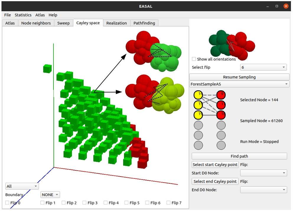
Figure 2: A screenshot of the EASAL software. The main screen shows the Cayley configuration space of an active constraint region, whose active constraint graph is shown on the bottom right. Green points represent valid configurations and the red points represent configurations that have streic collisions. We show two Cartesian configurations of the same Cayley point. The solid edges on the shown Cartesian configurations represent active constraints between the atoms they connect and the dotted edges represent the chosen Cayley parameters. See Section 2.4.

2.5 EASAL Variants and their Sampling Distributions

EASAL’s flexibility is demonstrated with a variety of sampling distributions in the Cayley space, which translates to sampling variants in the Cartesian space. EASAL-1 samples the Cayley space uniformly, skewing the distribution towards lower dimensional or lower energy regions. EASAL-2 uses a step size inversely proportional to the Cayley parameter value, resulting in more dense sampling in the interiors of active constraint regions. EASAL-3 uses a step size linearly proportional to the Cayley parameter value, resulting in dense sampling close to the boundaries of active constraint regions. EASAL-Jacobian uses a sophisticated Cayley sampling method [3] to force uniform sampling in the Cartesian space. It recursively and adaptively computes the next Cayley step size and direction using a computation of the Jacobian of the Cartesian-Cayley map to achieve this goal. Figure 3 shows the effect of sampling using different variants of EASAL on a typical randomly chosen 2D active constraint region.

(a) EASAL-1

(b) EASAL-2

(c) EASAL-3

(d) EASAL-Jacobian

(e) EASAL-1

(f) EASAL-2

(g) EASAL-3

(h) EASAL-Jacobian

Figure 3: Comparison of sampling distribution in Cayley (top row) v/s. Cartesian space (bottom row) in variants of EASAL for a 2D active constraint region in the atlas with the example in Figure 1 as input. The axes in the top figures are the two Cayley parameters. In the bottom figures, the projection is on the $xy$ coordinates of the centroid of the second point-set with the centroid of the first point-set fixed at the origin. See Section 2.5.

3 Results

Section 3.1 describes the experimental setup. Section 3.2 discusses the key measurements used to compare the different sampling algorithms in this paper. Section 3.3 discusses the performance of the sampling algorithms at uniform coverage, in terms of their speed, efficiency and accuracy. Section 3.4 discusses their performance at accurately covering lower dimensional regions. Section 3.5 illustrates the advantages of EASAL’s flexibility in terms of being able to restrict sampling to specified macrostates.

3.1 Experimental Setup

We compare the performance of five sampling algorithms, MC, EASAL-1, EASAL-2, EASAL-3, and EASAL-Jacobian with two identical transmembrane helices, each with 11 residues and 20 atoms as input (see Figure 1).

3.1.1 Metropolis Monte Carlo Experimental Setup

Metropolis Monte Carlo (MC) is an importance sampling method that generates an ensemble according to the Boltzmann factor. MC simulations were performed in order to explore the conformational space that is accessible by translational and rotational random steps of rigid helices. In all simulations reported, protein transmembrane alpha-helices were held rigid. The rigid body MC simulation was implemented in the HARLEM program [23] on a machine with Intel(R) Core(TM) i5-2540 CPU.

Move Sets: Trial conformations of rigid bodies are generated by a basic move set of a small translational and rotational displacement. The maximum step size for both types of displacements follow a well known criterion of the MC acceptance ratio. This criterion establishes that for optimum sampling the acceptance ratio should be around 50% of the trial moves. However, from our experience this high ratio of acceptance generates random structures with small conformational fluctuations. In order to overcome high energy barriers we implemented a move set based on the exponential distribution of the maximum step size of translation and rotation. The purpose of this move set is to randomly generate trial conformations with higher probability to jump over the energy barrier.

Moreover, analyzing MC trajectories showed that low energy conformations of different energy basins are conformationally different by the rotation around the principal axis of a rigid helix. Using this information we included in our MC implementation a move set in which a helix is randomly rotated around its principal axis.

Scoring Energy: The inter-molecular energy $E_{int}$ of a structure model in this work is calculated as follows:

$$E_{int}=w_{1}E_{pairwise}+w_{2}E_{steric}+w_{3}E_{mem}+w_{4}E_{vol}+w_{5}E_{solvation}$$ (1)

where $E_{pairwise}$ is the pairwise distance-based potential of the mean force of interaction between two residues, $E_{steric}$ is the steric overlap energy, $E_{mem}$ is the energy term that constrains the transmembrane helices to the membrane plane, $E_{vol}$ prevents the helix mass center from sampling farther than a radius of 15 Å, and $E_{solvation}$ accounts for the interaction of amino acids in different regions of the lipid bilayer.

3.1.2 EASAL Experimental Setup

With $d_{ij}$, the distance between the centers of atoms $i$ and $j$, and $r_{i}$ and $r_{j}$, the radii of atoms $i$ and $j$ respectively, we set the input pairwise distance component, for EASAL, as follows. For all atom pairs $(i,j)$ belonging to different rigid molecular components, the steric collision distance was set to $d_{ij}>0.8*(r_{i}+r_{j})$, the distance beyond which Lennard-Jones interactions are no longer relevant was set to $d_{ij}<r_{1}+r_{2}+0.9$, and the distance between these two is the Lennard-Jones well. The EASAL results were generated using its the curated opensource, software implementation, [4] (software available at http://bitbucket.org/geoplexity/easal, see also video https://cise.ufl.edu/~sitharam/EASALvideo.mpeg, and user guide https://bitbucket.org/geoplexity/easal/src/master/CompleteUserGuide.pdf). The EASAL experiments were run on an Intel(R) Core(TM) 2 Quad Q9450 @ 2.66GHz CPU with 3.9 GB of RAM. With this setup, sampling with EASAL1 took 3 hours 8 minutes, EASAL2 took 4 hours 24 minutes, EASAL3 took 10 hours 20 minutes, and EASAL-Jacobian took 14 hours 22 minutes.

3.1.3 Reference Grid for Uniform Coverage

In our experiments, uniform coverage is measured over a uniform grid in the Cartesian space. The angle parameters in the Cartesian space are represented in Euler angles (ZXZ). The grid is bounded along the 6 different Cartesian directions as follows, $X,Y:[-20$\mathrm{\SIUnitSymbolAngstrom}$,20$\mathrm{\SIUnitSymbolAngstrom}$]$, $Z:[-3.5$\mathrm{\SIUnitSymbolAngstrom}$,3.5$\mathrm{\SIUnitSymbolAngstrom}$]$ $\phi,\psi:[-\pi,\pi]$, and the inter principal-axis angle $\theta:[0^{\circ},30^{\circ}]$, where $\theta=a\cos(uv)$ with $u$ and $v$ the principal axis of the two helices.

3.1.4 MultiGrid: A Reference Grid for Weighted Coverage

To compare the performance of the sampling algorithms at being able to densely sample lower energy regions, we define a new reference grid, called MultiGrid. In MultiGrid, each grid point with $l$ active constraints (pairs of atoms in the Lennard-Jones’ well) is weighted by $l$, thus favoring lower dimensional, lower energy regions.

3.2 Key Measurements

We describe the key measurements used to compare MC with EASAL variants for the different sampling characteristics described in the introduction.

3.2.1 Measurements for Uniform Coverage

We measure the accuracy, efficiency, and speed of the sampling algorithms for covering the uniform grid described in Section 3.1.3. To measure the speed, we use the number of samples required by the sampling algorithms.

The accuracy of the different sampling algorithms at uniform coverage is measured using the epsilon coverage. An $\varepsilon$-cube is a cube centered around a grid point with a range of $2\varepsilon$ in each of the 6 dimensions (see Figure 4). The accuracy of uniform coverage is the percentage of $\varepsilon$-cubes covered by at least one sample point.

Since each of the sampling algorithms uses different number of samples, accuracy measures need to be normalized by the number of samples. We do this by defining the $\varepsilon$-cube for a sampling algorithm based on the number of samples. The value of $\varepsilon$ is set to:

$$\varepsilon:=\lceil\frac{\sqrt[6]{\frac{\Gamma}{\sigma}}}{2}\rceil$$

where $\Gamma$ is the total number of grid points and $\sigma$ is the number of EASAL/MC sample points. To compute $\varepsilon$-coverage, we assign each EASAL/MC sample to its closest grid point. Call those grid points EASAL/MC-mapped grid points. We say that a grid point $p$ is covered by EASAL/MC if there is at least one EASAL/MC -mapped grid point within the $\varepsilon$-cube centered around $p$. The better sampling algorithm will have greater $\varepsilon$-coverage.

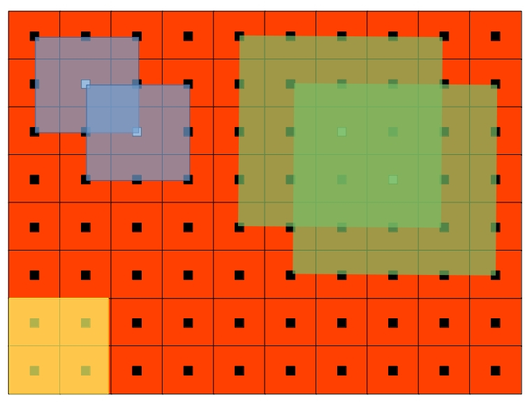
Figure 4: Illustration of epsilon cubes on a 2 dimensional grid. Black dots represent grid points, each of which is one step size away from its neighbor in every dimension. Red squares around the grid points are grid cubes. The shaded blue and green areas represent $\varepsilon$-cube and $\varepsilon+1$-cubes respectively, centered around the grid point in the middle of the cube (highlighted in white instead of black). The $\varepsilon$ and the $\varepsilon+1$ cubes extend 1 and 2 step sizes respectively from the center grid point in every dimension. As can be seen, there is significant overlap between epsilon cubes of neighboring points. The shaded yellow area represents a coarse grid cube. See Section 3.2.1

Efficient coverage requires sampling algorithms to minimize repeated samples by using as few samples as possible to cover an $\varepsilon$-cube (ideally only 1). We define two measures of efficiency. The first $\mu_{1}$, is the ratio of $\varepsilon$-cubes sampled efficiently (with exactly 1 sample) to the ratio of $\varepsilon$-cubes sampled inefficiently (with more than 1 samples). The second $\mu_{2}$, is the ratio of the number of $\varepsilon$-cubes sampled efficiently (with exactly 1 sample) to the total number of samples in all other cubes.

We measure the speed of the different sampling algorithms using the number of samples required to achieve a certain $\epsilon$-coverage. The better algorithm uses fewer number of samples.

3.2.2 Measurements for Weighted Coverage of Lower Energy Regions

To measure the accuracy of weighted coverage with respect to lower energy regions, we compare the distribution of samples in the different sampling algorithms to the distribution of samples in the reference MultiGrid.

A key measure here is the distribution ratio of an active constraint region, which is the ratio of the number of samples in the region to the total number of samples in all regions in the atlas. We compare the distribution ratios of EASAL variants and MC to MultiGrid.

3.2.3 Measurements for Localized Sampling of Individual Constraint Regions

To demonstrate EASAL’s sampling flexibility which allows individual active constraint regions to be sampled quickly, we compare the number of samples required to sample a macrostate to the total number of samples in all macrostates. Since MC does not have the ability to restrict sampling to macrostates, in the worst case, it may need to sample the entire energy landscape to sample a single macrostate.

Let $s_{1}$ be the number of samples in a specific but randomly chosen three-dimensional region and $s_{2}$ be the number of samples in all ancestor regions with one active constraint that lead to the three-dimensional region. The ratio percentage is $\frac{s_{1}}{s_{2}}\times 100$. Ratio percentage is a measure of the percentage of samples in an ancestor 5-dimensional node that will end up in a given 3-dimensional active constraint region.

3.3 Uniform Coverage: Accuracy, Efficiency, and Speed

In this experiment, we compare the performance of the different sampling algorithms at covering the uniform grid described in Section 3.1.3. The best method should have the highest epsilon coverage with the fewest number of samples. Table 1 summarizes the coverage results, in terms of speed and accuracy for MC and 4 EASAL variants. MC gives the best coverage at $99.96\%$, but requires 100 million samples to do the same. Compare this to EASAL-Jacobian, which gives similar coverage with $99.53\%$ with a hundredth the number of samples as MC. EASAL-2 gives a very good coverage of 92.42% with only 40k samples (0.04% of MC).

Table 1: Comparison of MC with EASAL variants for speed and accuracy of uniform coverage, with the two transmembrane helices shown in Fig. 1 as input. See Section 3.3.

sampling method	EASAL-1	EASAL-2	EASAL-3	EASAL-Jacobian	MC	Grid	MultiGrid
$\varepsilon$ value	$\lceil 0.97\rceil$	$\lceil 1.14\rceil$	$\lceil 1.20\rceil$	$\lceil 0.66\rceil$	$\lceil 0.31\rceil$	N/A	N/A
$\varepsilon$ coverage	92.06%	92.42%	74.08%	99.53%	99.96%	N/A	N/A
Number of Samples	100k	40k	30k	1 million	100 million	6 million	12 million

To compare the sampling algorithms in terms of efficiency at covering the uniform grid, Figure 5 plots the number of sample points $\nu$ (from the different sampling algorithms) that lie in an $\varepsilon$-cube against the number of $\varepsilon$-cubes having $\nu$ EASAL/MC-mapped, sample points in them. A good sampling algorithm (one that minimizes repeated samples) should have the fewest number of sample points per $\varepsilon$-cube mapped to the same epsilon cube. In the plot, this would appear as a histogram skewed heavily to the left. As can be seen, EASAL-1, EASAL-2, and EASAL-3 have peaks at the left-most part of the histogram, indicating that they minimize discarded samples better than MC and EASAL-Jacobian.

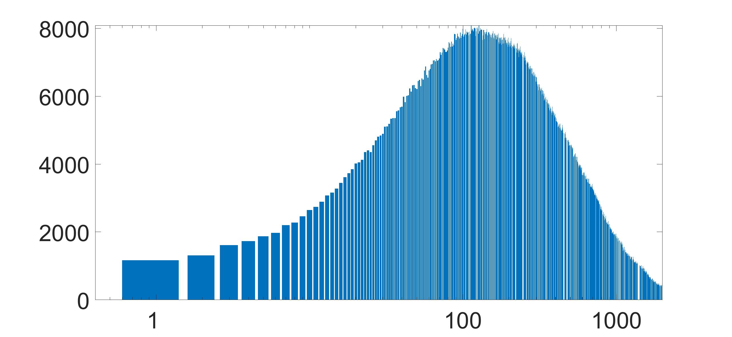
(a) MC

(b) EASAL-Jacobian

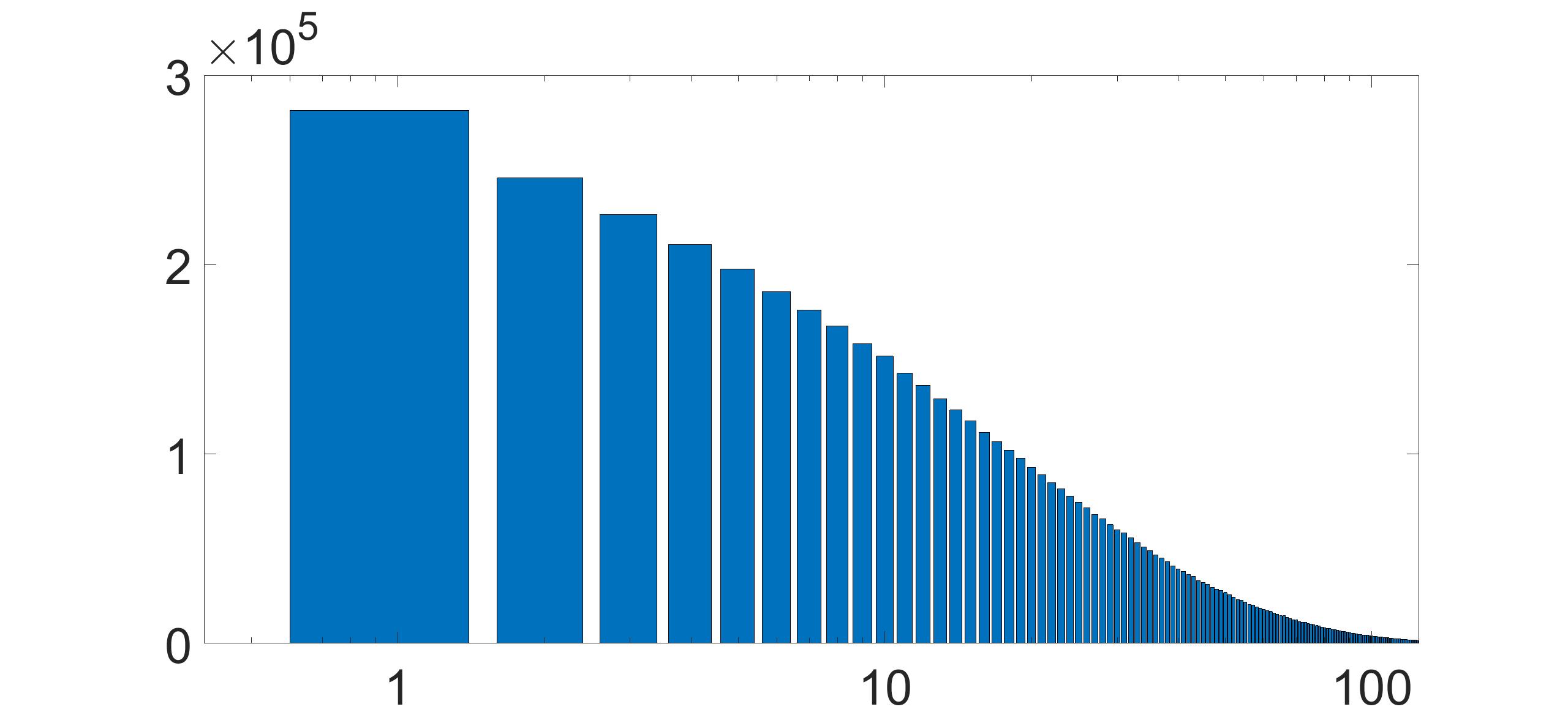
(c) EASAL-1

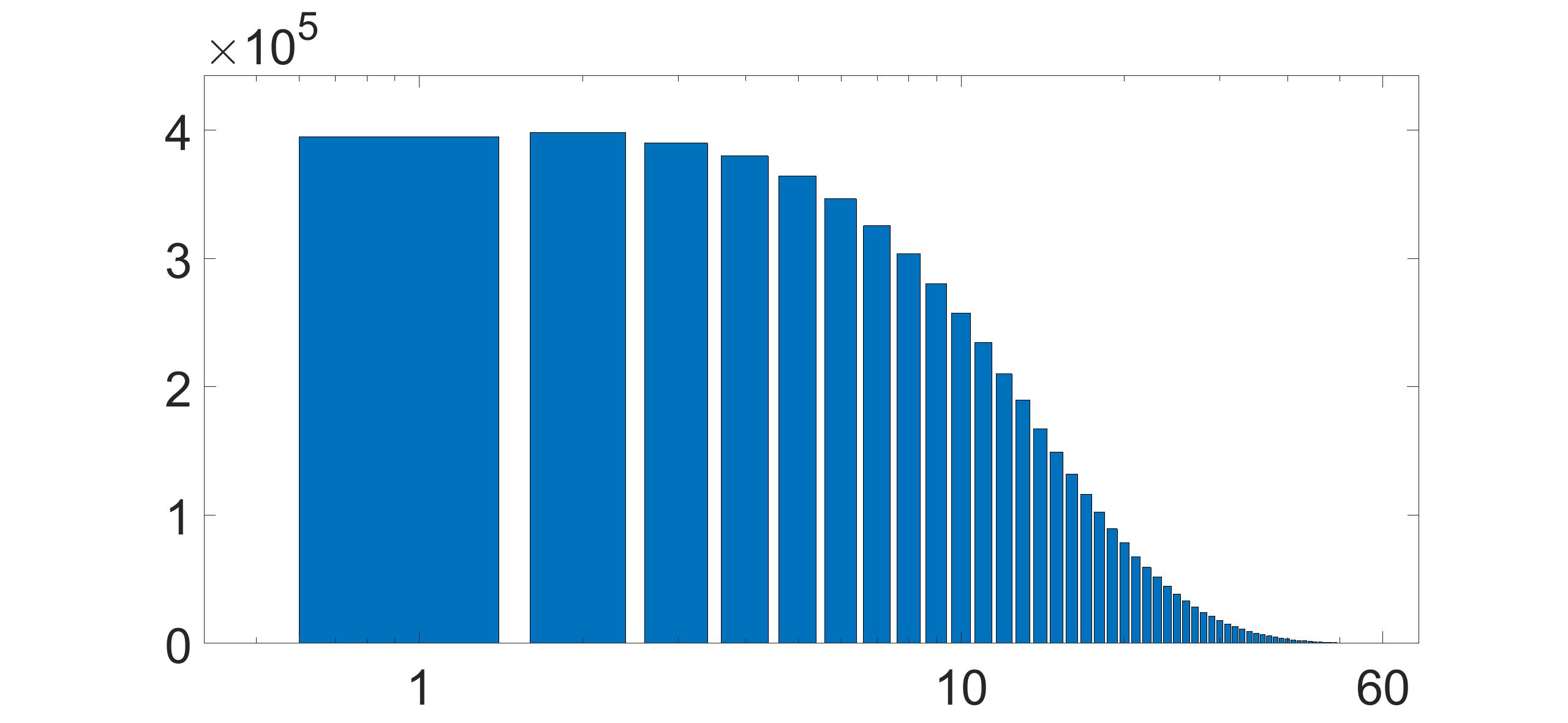
(d) EASAL-2

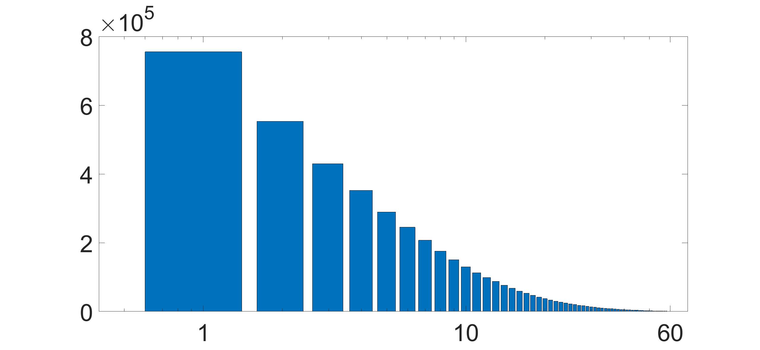
(e) EASAL-3

Figure 5: The horizontal axis shows the number of sample points $\nu$ that lie in $\varepsilon$-cubes, and the vertical axis shows the number of $varepsilon$-cubes having $\nu$ EASAL/MC-mapped points inside of them. See Section 3.3.

The next step is trying to find an $\varepsilon$ for which we get denser coverage from all the sampling algorithms. Figure 6 plots the number of sample points $\nu$ (from the different sampling algorithms) that lie in an $\varepsilon+1$-cube against the number of $varepsilon+1$-cubes having $\nu$ EASAL/MC-mapped, sample points in them. As can be seen, expanding the size of the $\varepsilon$ cube results in much denser coverage from all the sampling algorithms, with EASAL-3 still being judicious with the number of samples per $\varepsilon$ cube.

(a) MC

(b) EASAL-Jacobian

(c) EASAL-1

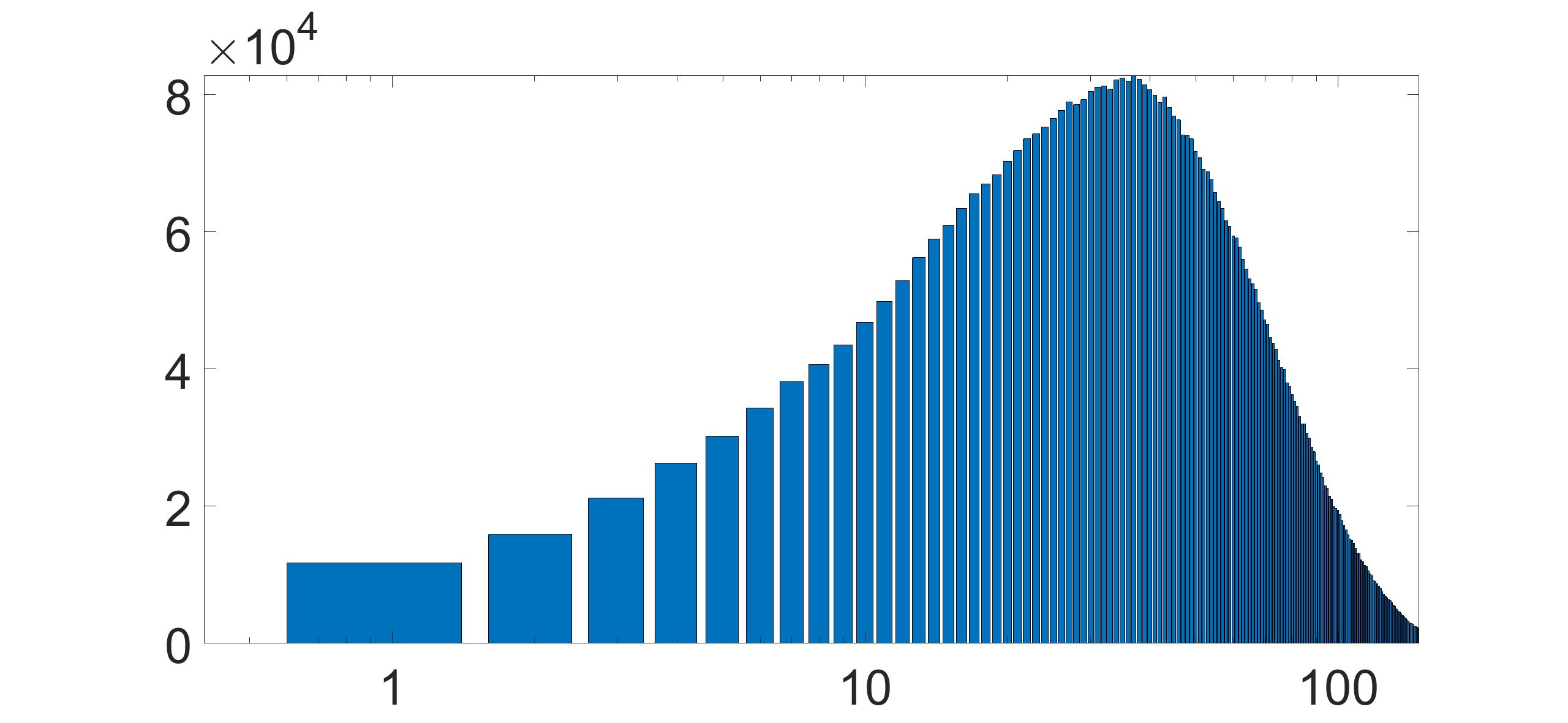
(d) EASAL-2

(e) EASAL-3

Figure 6: The horizontal axis shows the number of sample points $\nu$ that lie in $\varepsilon+1$-cubes, and the vertical axis shows the number of $\varepsilon+1$-cubes having $\nu$ EASAL/MC-mapped points inside of them. See Section 3.3.

Table 2: Comparison of MC with EASAL variants for efficiency of uniform coverage, with the two transmembrane helices shown in Fig. 1 as input. We show the efficiency at both $\varepsilon$-coverage and $\varepsilon+1$-coverage. See Section 3.3.

Sampling Algorithm	$\varepsilon$-coverage		$\varepsilon+1$-coverage
	$\mu_{1}$	$\mu_{2}$	$\mu_{1}$	$\mu_{2}$
MC	0.0002	0	0.00001	0
EASAL-1	0.04	2.81	0.008	0.14
EASAL-2	0.06	9.87	0.002	0.29
EASAL-3	0.01	25.1	0.02	5.1
EASAL-Jacobian	0.002	0.001	0.00001	0.00007

Next, we use the two efficiency measures $\mu_{1}$ and $\mu_{2}$ described in Section 3.2.1, to compare the sampling algorithms in terms of their efficiency at covering the uniform grid. Table 2 summarizes the results for coverage of $\varepsilon$ and $\varepsilon+1$ cubes. EASAL variants have have better coverage efficiency in terms of both measures.

3.4 Accuracy of Weighted Coverage

The objective of this experiment is to compare the performance of the sampling methods at covering low energy regions. Figure 7 shows a 2-dimensional projection of the Cartesian configuration space of the input transmembrane helices described in the experimental setup as sampled by different methods. The projection is on the $xy$ coordinates of the centroid of the second helix with the centroid of the first helix fixed at the origin. There are no samples on the outer rim since since we have set the inter helical angle to be less than $30^{\circ}$. There are also no samples in the center of the plots because the configurations in this area have steric collisions due to the helix mass center of the molecules being close to each other.

The sampling algorithm that covers lower energy region better, should have a distribution of samples that resembles the MultiGrid figure closely. Notice that EASAL-Jacobian and EASAL-2 approximate MultiGrid better than MC.

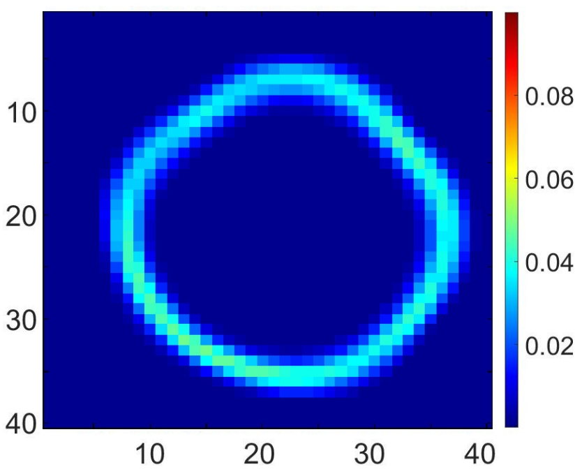
(a) Grid

(b) MC

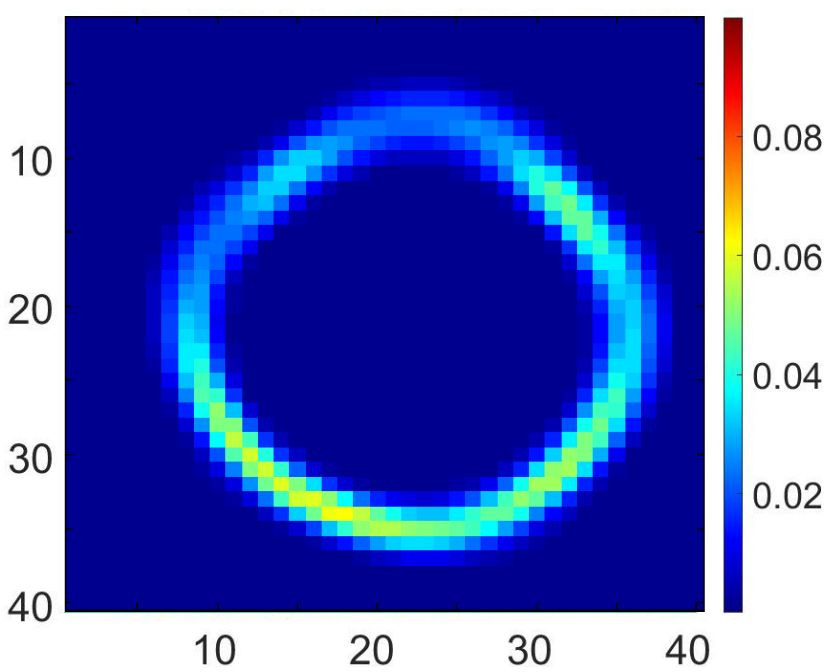
(c) MultiGrid

(d) EASAL-Jacobian

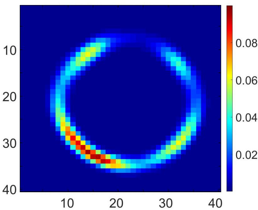
(e) EASAL1

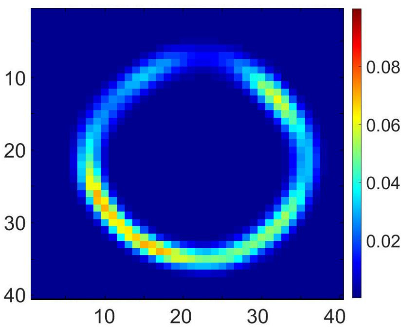
(f) EASAL2

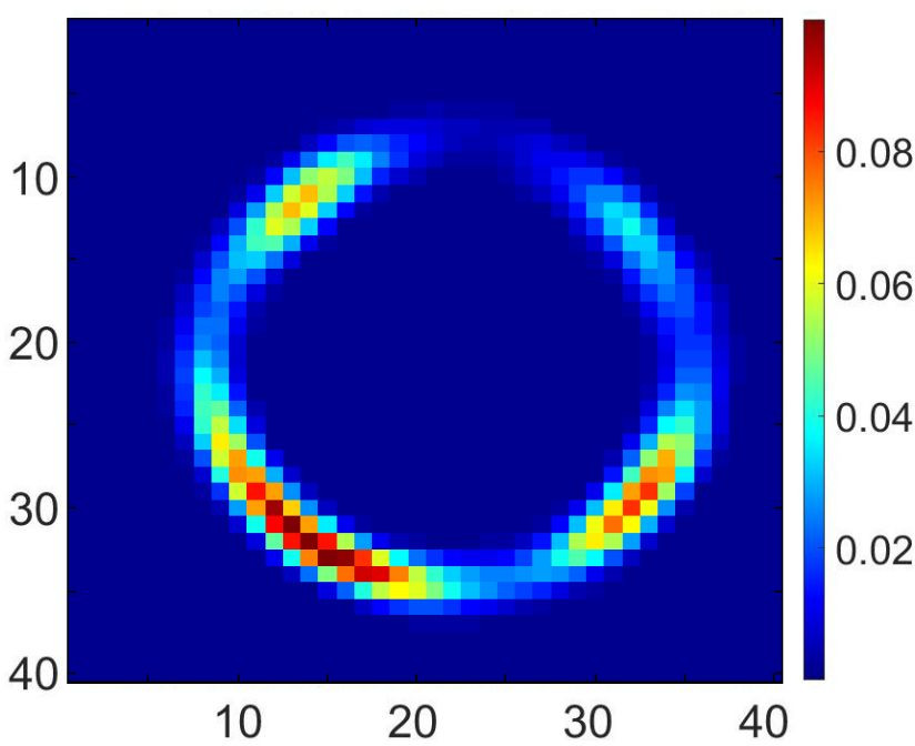
(g) EASAL3

Figure 7: Projection in $R^{2}$ of a configuration space for the example helices described in Section 3.1, as sampled by different methods. The projection is on the $xy$ coordinates of the centroid of the second helix, with the centroid of the first helix fixed in the center. The color scale on the right of each figure corresponds to the number of sampled points in a $\varepsilon$-sized cube centered around the grid point $(x,y)$. See Section 3.4.

In the next plot, we still take the $xy$ projection as before, but on a coarser grid with 100 grid cubes (10 by 10) instead of the original 1600 grid cubes (40 by 40 used in Figure 7). Figure 8 plots the percentage of samples in an $xy$-cube. The percentage of samples is computed by summing all samples of subregions with a specific $x,y$ and dividing it by the total number of samples.

Since MultiGrid densely samples lower energy regions, the portions of the MultiGrid plot with darker spots are the lower energy regions. As can be seen, the EASAL variants sample these lower energy regions much denser than MultiGrid. In contrast, MC and Grid, which are similar to each other, sample these areas sparsely.

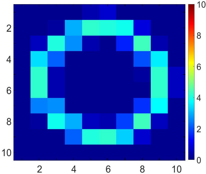
(a) Grid %

(b) MC %

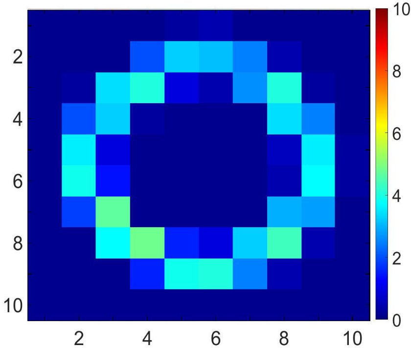
(c) MultiGrid %

(d) EASAL_Jacobian %

(e) EASAL1 %

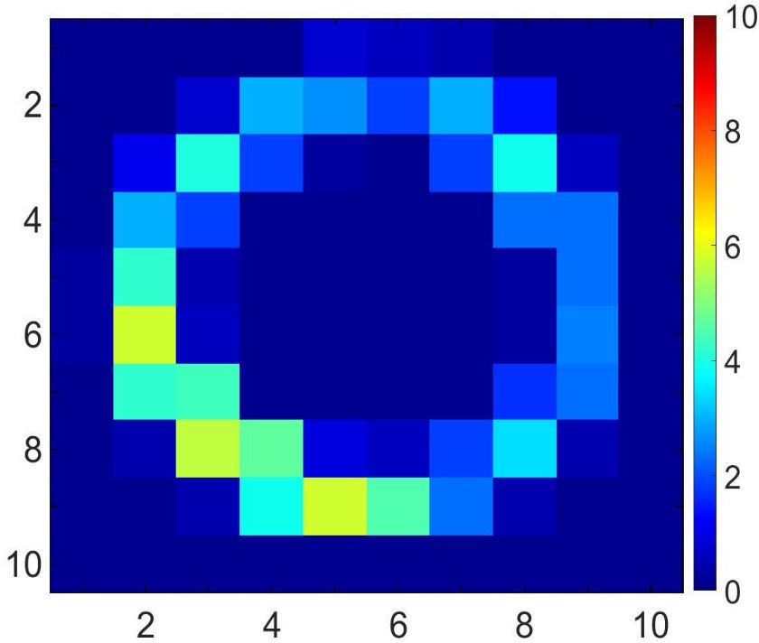
(f) EASAL2 %

(g) EASAL3 %

Figure 8: Projection in $R^{2}$ of a configuration space for the example helices described in Section 3.1, as sampled by different methods. The projection is on the $xy$ coordinates of the centroid of the second helix, with the centroid of the first helix fixed in the center. We use a coarse $xy$ grid as described in the text. The color scale on the right of each figure corresponds to the percentage of samples in the coarse $xy$ region. The percentage of samples is computed by summing all samples of subregions with a specific $x,y$ and dividing it by the total number of samples. See Section 3.4.

Figure 9 plots the distribution of samples across different active constraint regions or atlas nodes. The atom indices of the two helices are shown as the rows and columns of a matrix. The $(row_{1},column_{1})$ entry represents a 5D active constraint region, where the active constraint is between the atom number $row_{1}$ on the first molecule and atom number $column_{1}$ on the second molecule. The color code gives the distribution ratio. The plot of atlas MultiGrid has higher distribution ratios for active constraint regions with where there are more lower energy configurations. Note that EASAL variants resemble distribution ratios of MultiGrid more than grid and MC distributions.

(a) Atlas MC

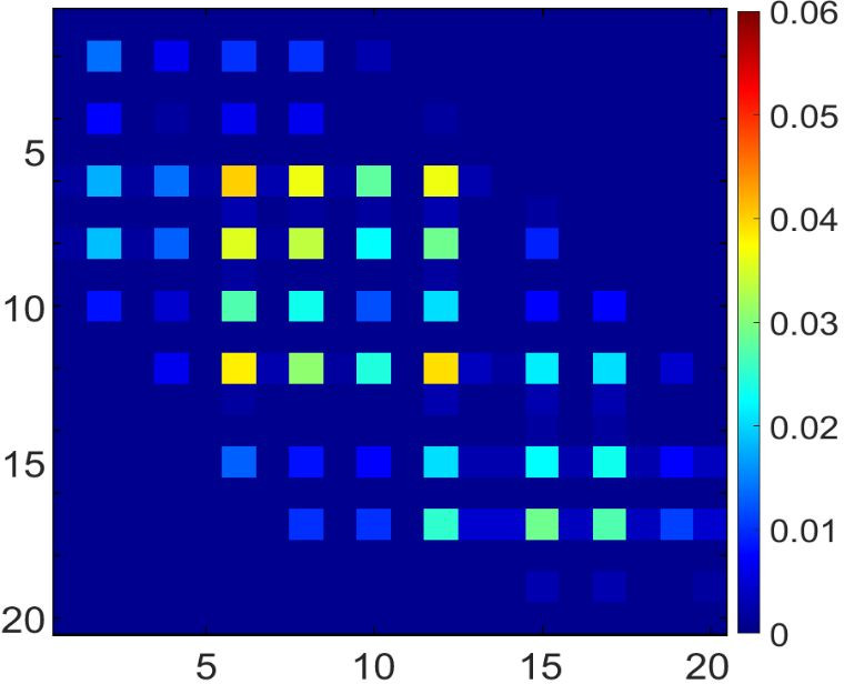
(b) Atlas Grid

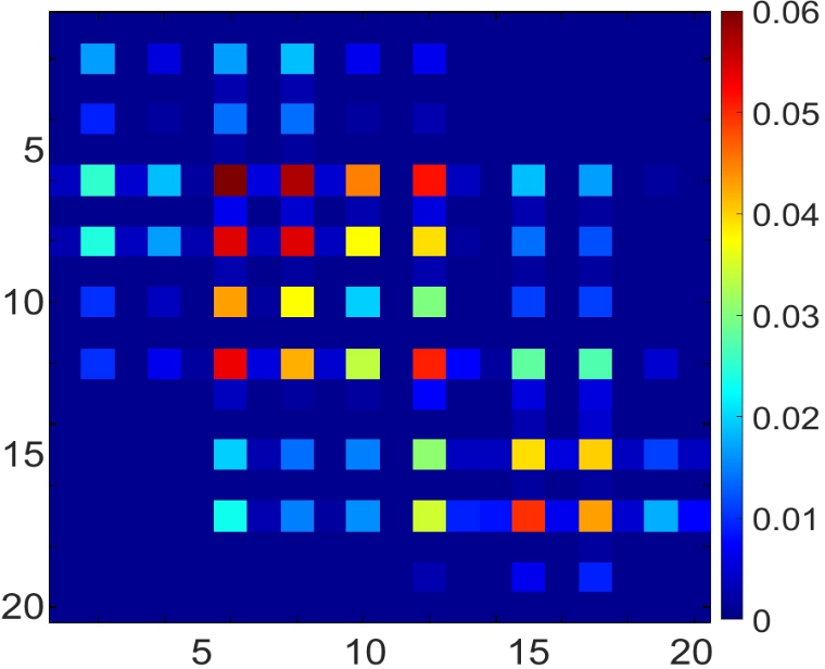
(c) Atlas MultiGrid

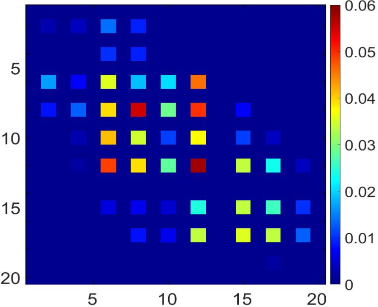
(d) EASAL-Jacobian

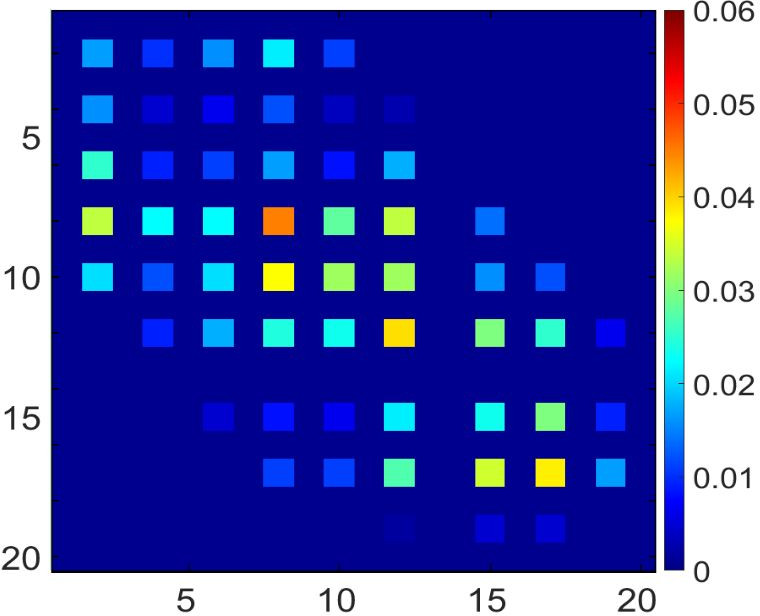
(e) EASAL-1

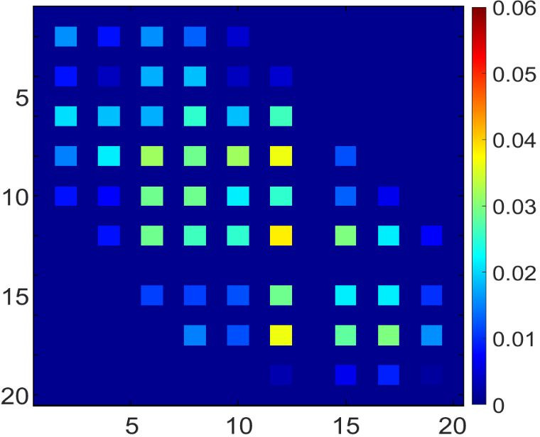
(f) EASAL-2

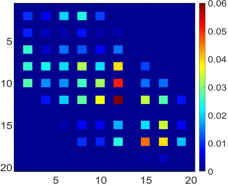
(g) EASAL-3

Figure 9: The atom indices of the two helices are shown as the rows and columns of a matrix. The $(row_{1},column_{1})$ entry represents a 5D active constraint region, where the active constraint is between the atom number $row_{1}$ on the first molecule and atom number $column_{1}$ on the second molecule. The color code gives the distribution ratio. The plot of atlas MultiGrid has higher distribution ratios for active constraint regions with where there are more lower energy configurations. Note that EASAL variants resemble distribution ratios of MultiGrid more than grid and MC distributions. See Section 3.5.

3.5 Localized Sampling of Individual Active Constraint Regions (macrostates)

The goal of this experiment is to demonstrate EASAL’s ability to restrict sampling to specified macrostates.

Table 3: Comparison of MC with EASAL variants in terms of ratio percentages. See Section 3.5.

Sampling method	EASAL-1	EASAL-2	EASAL-3	EASAL-Jacobian	MC
Ratio percentage	3.56%	5.17%	2.97%	3.45%	1.29%

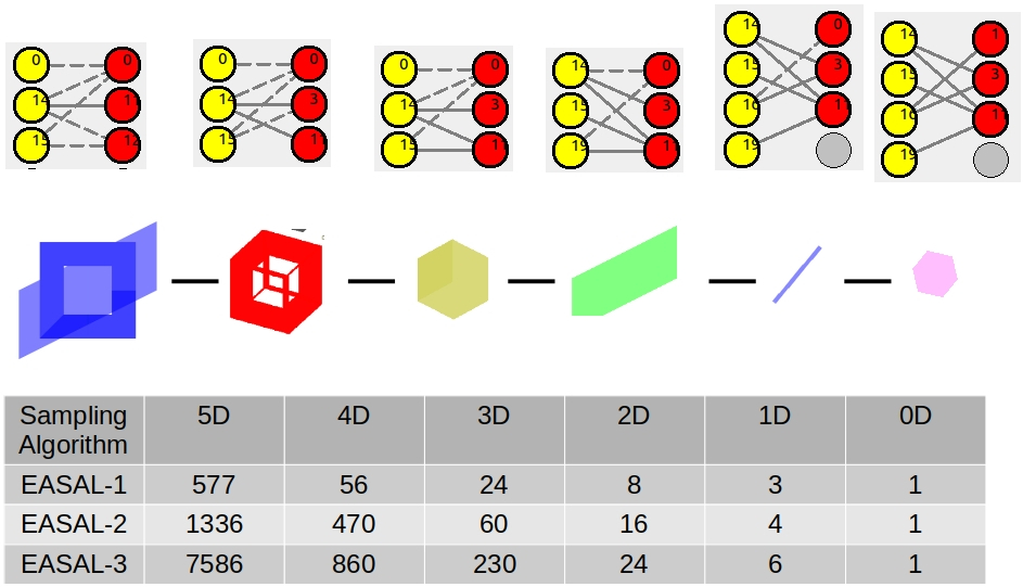
Figure 10: A path in a the EASAL atlas from a 5D to a 0D node, showing the active constraint graphs of each node and the number of samples required to sample each region with different variants of EASAL. See Section 3.5.

Table 3 summarizes the ratio percentages of MC and EASAL variants for sampling the two transmembrane helices described in the experimental setup. The ratio percentage gives a measure of the percentage of samples required to directly sample a 3D region as compared to trying to sampling the entire energy landscape. For instance, EASAL-1 has ratio percentage of 3.56%, this means that EASAL-1 would need only 3.56% of samples to sample a 3D active constraint region or macrostate directly, as compared to compared to sampling portion of the configuration space starting with a 5D active constraint region and reaching the given 3D region. EASAL’s ability to localize sampling reduces the number of samples required to sample particular macrostates.

This is further illustrated in Figure 10 with a concrete example. We show a path in the EASAL atlas from a 5D to a 0D active constraint region along with the number of samples required to sample each of them using different EASAL variants. The table in Figure 10 shows how being able to localize sampling to a particular macrostate can reduce the number of samples required, especially when sampling the lower dimensional regions. For instance, if we are interested in only sampling the 3D region shown in the figure, the EASAL variants would need 24, 60, and 230 samples. However, in the absence of this ability, we would have to sample the entire configuration space to sample just this region, which is the case with MC.

However, as shown in the paper [2], EASAL gives the best accuracy when starting sampling from 5D active constraint regions. When the starting dimension of sampling goes down, EASAL’s accuracy in terms of the number of 0D regions discovered goes down. Despite this, EASAL is still able to discover a respectable number of 0D active constraint regions even with a very coarse sampling step size and starting from the 3D region shown in Table 4.

Table 4: The number of 0D regions discovered with EASAL-1 sampling, when starting sampling from the 3D region shown in Figure 10 with varying step sizes.

Step size	0D regions discovered
0.4	144
0.8	122
1.2	82
1.6	72
2	60

4 Discussion

The uniform grid described earlier, can be sampled by brute force to get good coverage. However, this uses a large number of samples and over 90% of these are typically discarded since they are high energy configurations (no active constraints). This method also finds it difficult to sample low energy (more than 1 active constraint) regions.

In the case of MC, the simulation has a tendency to sample around a localized sub-set of low energy configurations that are located close to each other. To ensure coverage, one needs to compensate for the lack of ergodicity by computationally intensive use of a large number of samples.

EASAL has flexibility in sampling distributions, but in all cases guarantees reasonable coverage of low energy regions even if they have low effective dimension. It tends to over-sample these lower energy regions (i.e, regions where more pairs of atoms are in their Leonard-Jones well). Hence EASAL can help MC to find high energy barriers and force the MC simulations to move to the locations of low energy basins. Macrostates with lower energy, which MC misses due to broken ergodicity, can be sampled using EASAL and used as a seed for MC in order to generate the free energy profile for the whole configuration space.

More precisely, we expect EASAL to be used to help evaluate/improve MC with the following path.

1. Run a coarse-grained version of MC with the usual energy function and a relatively small number of samples

2. Run EASAL with constraints extracted from the MC energy function, verify that the space sampled by EASAL encompasses the relevant space.

3. List description of macrostates that MC missed, and give an estimate of the volume of the regions.

4. Compute energy on these regions, and if low, then run MC seeded on these (lower volume) regions (from which larger volume regions can be reached), in order to generate the free energy profile for the whole configuration space.

5. Compare new trajectories with old MC trajectories.

5 Conclusion

We compare the sampling characteristics of the EASAL methodology to the traditional MonteCarlo sampling, using custom-designed measurements, for sampling the the assembly landscape of 2 transmembrane helices, with short-range pair-potentials. We demonstrate that variants of EASAL provide good coverage of narrow regions of low potential energy and low effective dimension with much fewer samples and computational resources than MC.

We provide promising avenues for combining the complementary advantages of the two methods, which can significantly improve the current state of the art of free energy and other integral computations, specifically for small assemblies. EASAL is tailored for such assemblies and can be used to improve accuracy and ergodicity guarantees for Monte Carlo trajectories. It can also help explain the behavior of MC trajectories by using EASAL to infer geometric and topological features of the configuration space.

EASAL can help MC find high energy barriers and force the simulations to move to the locations of low energy basins. Finally, lower energy regions located by EASAL can be used as seeds for MC trajectories, to speed up traversal of the entire configuration space.

References

- [1] Aysegu Ozkan and Meera Sitharam. Easal: Efficient atlasing, analysis and search of molecular assembly landscapes. In Proceedings of the ISCA 3rd International Conference on Bioinformatics and Computational Biology, BICoB-2011, 2011.
- [2] Rahul Prabhu, Meera Sitharam, Aysegul Ozkan, and Ruijin Wu. Atlasing of Assembly Landscapes using Distance Geometry and Graph Rigidity, 2020. Preprint on arXiv https://arxiv.org/abs/1203.3811.
- [3] Aysegul Ozkan and Meera Sitharam. Best of Both Worlds: Uniform sampling in Cartesian and Cayley Molecular Assembly Configuration Space, 2014. Preprint on arxiv https://arxiv.org/abs/1409.0956.
- [4] Aysegul Ozkan, Rahul Prabhu, Troy Baker, James Pence, Jorg Peters, and Meera Sitharam. Algorithm 990: Efficient atlasing and search of configuration spaces of point-sets constrained by distance intervals. ACM Trans. Math. Softw., 44(4):48:1–48:30, July 2018.
- [5] Ruijin Wu, Aysegul Ozkan, Antonette Bennett, Mavis Agbandje-Mckenna, and Meera Sitharam. Robustness measure for an adeno-associated viral shell self-assembly is accurately predicted by configuration space atlasing using easal. In Proceedings of the ACM Conference on Bioinformatics, Computational Biology and Biomedicine, BCB ’12, pages 690–695, New York, NY, USA, 2012. ACM.
- [6] Ruijin Wu, Rahul Prabhu, Antonette Bennett, Aysegul Ozkan, Mavis Agbandje-McKenna, and Meera Sitharam. Prediction of Crucial Interaction for Icosahedral Capsid Self-Assembly by Configuration Space Atlasing using EASAL, 2020. Preprint available on arXiv: https://arxiv.org/abs/2001.00316.
- [7] Dina Duhovny, Ruth Nussinov, and Haim J. Wolfson. Efficient unbound docking of rigid molecules. In Roderic Guigó and Dan Gusfield, editors, Algorithms in Bioinformatics, pages 185–200, Berlin, Heidelberg, 2002. Springer Berlin Heidelberg.
- [8] Garland R. Marshall and Ilya A. Vakser. Protein-Protein Docking Methods, pages 115–146. Springer US, Boston, MA, 2005.
- [9] Nelly Andrusier, Ruth Nussinov, and Haim J. Wolfson. Firedock: Fast interaction refinement in molecular docking. Proteins: Structure, Function, and Bioinformatics, 69(1):139–159, 2007.
- [10] Nelly Andrusier, Efrat Mashiach, Ruth Nussinov, and Haim J. Wolfson. Principles of flexible protein–protein docking. Proteins: Structure, Function, and Bioinformatics, 73(2):271–289, 2008.
- [11] Sandor Vajda and Dima Kozakov. Convergence and combination of methods in protein-protein docking. Current Opinion in Structural Biology, 19(2):164 –170, 2009.
- [12] David W. Ritchie. Recent progress and future directions in protein-protein docking. Current Protein and Peptide Science, 9:1–15, 2008. doi:10.2174/138920308783565741.
- [13] Joel Janin. Protein-protein docking tested in blind predictions: the capri experiment. Mol. BioSyst., 6(12):2351–2362, 2010.
- [14] Juan Fernández-Recio and Michael J. E. Sternberg. The 4th meeting on the critical assessment of predicted interaction (capri) held at the mare nostrum, barcelona. Prot.Struct.Func.Bioinfo., 78(15):3066, 2010. 3065.
- [15] E. Katchalskikatzir, I. Shariv, M. Eisenstein, A. A. Friesem, C. Aflalo, and I. A. Vakser. Molecular-surface recognition - determination of geometric fit between proteins and their ligands by correlation techniques. Proceedings of the National Academy of Sciences of the United States of America, 89(6):2195–2199, 1992. Hj053 Times Cited:484 Cited References Count:29.
- [16] Sergei Bespamyatnikh, Vicky Choi, Herbert Edelsbrunner, and Johannes Rudolph. Accurate protein docking by shape complementarity alone. Manuscript, Duke Univ., Durham, NC, 2004.
- [17] D. Schneidman-Duhovny, Y. Inbar, R. Nussinov, and H. J. Wolfson. PatchDock and SymmDock: servers for rigid and symmetric docking. Nucleic Acids Res., 33(Web Server issue):W363–367, Jul 2005.
- [18] T Lazaridis and M Karplus. Effective energy function for proteins in solution. Proteins, 35(2):133–152, 1999.
- [19] Themis Lazaridis. Effective energy function for proteins in lipid membranes. Proteins, 52(2):176–192, 2003.
- [20] Wonpil Im, Michael Feig, and Charles L Brooks. An implicit membrane generalized born theory for the study of structure, stability, and interactions of membrane proteins. Biophysical Journal, 85(5):2900–2918, 2003.
- [21] Tzee-Char Kuo. On thom-whitney stratification theory. Mathematische Annalen, 234:97–107, 1978. 10.1007/BF01420960.
- [22] M. Sitharam and H.Gao. Characterizing graphs with convex cayley configuration spaces. Discrete and Computational Geometry, 2010.
- [23] IV Kurnikov, K Speranskiy, and MG Kurnikova. Harlem (hamiltonians to research large molecules). software package, 2001. https://crete.chem.cmu.edu/index.php/software/harlem-software.