Bayesian Lattice Filters for Time-Varying Autoregression and Time-Frequency Analysis
Wen-Hsi Yang111CSIRO Computational Informatics, Ecosciences Precinct, GPO Box 2583, Brisbane QLD 4001, Australia, Wen-Hsi.Yang@csiro.au, Scott H. Holan222(To whom correspondence should be addressed) Department of Statistics, University of Missouri, 146 Middlebush Hall, Columbia, MO 65211-6100, holans@missouri.edu, Christopher K. Wikle333Department of Statistics, University of Missouri, 146 Middlebush Hall, Columbia, MO 65211-6100, wiklec@missouri.edu
Abstract
Modeling nonstationary processes is of paramount importance to many scientific disciplines including environmental science, ecology, and finance, among others. Consequently, flexible methodology that provides accurate estimation across a wide range of processes is a subject of ongoing interest. We propose a novel approach to model-based time-frequency estimation using time-varying autoregressive models. In this context, we take a fully Bayesian approach and allow both the autoregressive coefficients and innovation variance to vary over time. Importantly, our estimation method uses the lattice filter and is cast within the partial autocorrelation domain. The marginal posterior distributions are of standard form and, as a convenient by-product of our estimation method, our approach avoids undesirable matrix inversions. As such, estimation is extremely computationally efficient and stable. To illustrate the effectiveness of our approach, we conduct a comprehensive simulation study that compares our method with other competing methods and find that, in most cases, our approach performs superior in terms of average squared error between the estimated and true time-varying spectral density. Lastly, we demonstrate our methodology through three modeling applications; namely, insect communication signals, environmental data (wind components), and macroeconomic data (US gross domestic product (GDP) and consumption).
Keywords: Locally stationary; Model selection; Nonstationary; Partial autocorrelation; Piecewise stationary; Sequential estimation; Time-varying spectral density.
1 Introduction
Recent advances in technology have lead to the extensive collection of complex high-frequency nonstationary signals across a wide array of scientific disciplines. In contrast to the time-domain, the time-varying spectrum may provide better insight into important characteristics of the underlying signal (e.g., Holan et al.,, 2010, 2012; Rosen et al.,, 2012; Yang et al.,, 2013, and the references therein). For example, Holan et al., (2010) demonstrated that features in the time-frequency domain of nonstationary Enchenopa treehopper mating signals may describe crucial phenotypes of sexual selection.
In general, time-frequency analyses can either proceed using a nonparametric or model-based (parametric) approach. The most common nonparametric approach is the short-time Fourier transform (i.e., windowed Fourier transform) which produces a time-frequency representation characterizing local signal properties (Gröchenig,, 2001; Oppenheim and Schafer,, 2009). Another path to time-frequency proceeds using smoothing splines (Rosen et al.,, 2009, 2012) or by parameterizing the spectral density to estimate the local spectrum via the Whittle likelihood (Everitt et al.,, 2013). Similarly, time-frequency can be achieved by applying smooth localized complex exponential (SLEX) functions to the observed signal (Ombao et al.,, 2001). In contrast to window based approaches, the SLEX functions are produced using a projection operator and are, thus, simultaneously orthogonal and localized in both time and frequency. Alternatively, one can use the theory of frames and over-complete bases to produce a time-frequency representation. For example, continuous wavelet transforms (Vidakovic,, 1999; Percival and Walden,, 2000; Mallat,, 2008) or Gabor frames (Wolfe et al.,, 2004; Feichtinger and Strohmer,, 1998; Fitzgerald et al.,, 2000) could be used. By introducing redundancy into the basis functions, these representations may provide better simultaneous resolution over both time and frequency.
Model-based approaches typically proceed through the time-domain in order to produce a time-frequency representation for a given nonstationary signal. In this setting common approaches include fitting piecewise autoregressive (AR) models as well as time-varying autoregressive (TVAR) models. The former approach assumes that the nonstationary signal is piecewise stationary. Consequently, the estimation procedure attempts to identify the order of the AR models along with the location of each piecewise stationary series. For example, Davis et al., (2006) propose the AutoPARM method using minimum description length (MDL) in conjunction with a genetic algorithm (GA) to automatically locate the break points and AR model order within each segmentation. In addition to providing a time-frequency representation, this approach also locates changepoints. Wood et al., (2011) propose fitting mixtures of AR models within each segment via Markov chain Monte Carlo (MCMC) methods. Their approach selects a common segment length and then divides the signal into these segments prior to implementation of the fitting procedure. Although such approaches may accommodate signals with several piecewise stationary structures, they lack the capability of capturing momentary shocks to the system (i.e., changes to the evolutionary structure that only occur over relatively few time points).
For many processes, TVAR models may provide superior resolution within the time-frequency domain for both large and small scale features through modeling time-varying parameters. To estimate the TVAR model coefficients, Kitagawa and Gersch, (1996) and Kitagawa, (2010) treat the coefficients as a stochastic process and model them using difference equations under the assumption of a maximum fixed order of the TVAR model. Their estimation procedure for the coefficients is then based on state-space models with smoothness priors. In this context, the innovation variances are treated as constant and estimated using a maximum likelihood approach. Subsequently, West et al., (1999) propose a fully Bayesian TVAR framework that simultaneous models the coefficients and the innovation variances using random walk models. Alternatively, by assuming a constant innovation variance, Prado and Huerta, (2002) model the coefficients and order of the TVAR model using random walk models. Further, to make the TVAR models stable, the constraint that the roots of the characteristic polynomial lie within the unit circle could be imposed. However, such an added condition makes estimation more complicated and computationally expensive.
To avoid these issues, we instead work with the partial autocorrelation coefficients (i.e., in the partial correlation (PARCOR) coefficient domain) and then use the Levinson recursion to connect the PARCOR coefficients and TVAR model coefficients (Kitagawa and Gersch,, 1996; Godsill et al.,, 2004). Godsill et al., (2004) model the PARCOR coefficients and innovation standard deviations using a truncated normal first-order autoregression and a log Gaussian first-order autoregression, respectively, with a given constant order. To estimate these values, a sequential Monte Carlo algorithm is used. Alternatively, as previously alluded to, by assuming a constant innovation variance, Kitagawa and Gersch, (1996) implement the smoothness prior within a lattice filter to estimate the PARCOR coefficients. After the PARCOR coefficients have been estimated, a constant innovation variance is estimated using a maximum likelihood approach. However, the former approach is computationally expensive and may suffer from the degeneracy problem (i.e., the collapse of approximations of the marginal distributions) when TVAR model order is large. In addition, certain hyperparameter values (i.e., the TVAR coefficients associated with the two latent models) may be sensitive to starting values and may require prior knowledge or expert supplied subjective information to achieve convergence (Godsill et al.,, 2004). Although the latter takes advantage of the lattice form to estimate the PARCOR coefficients, estimation of the innovation variance is achieved outside of the lattice structure; that is, the estimation procedure is a two-stage method. Importantly, this approach is designed for a constant innovation variance and cannot deal with time-dependent innovation variances. As such, we propose a novel approach that addresses these issues within a fully Bayesian context.
Kitagawa, (1988) and Kitagawa and Gersch, (1996) constitute the first attempts at utilizing the lattice structure to estimate the coefficients of a TVAR model when the innovations follow a Gaussian distribution with mean zero and constant variance. At each stage of the lattice filter, they assume that the residual at each time between the forward and backward prediction errors follows a Cauchy distribution, and that the PARCOR coefficient is modeled as a Gaussian random walk. This produces a non-Gaussian state space model at each stage and thus, a numeric algorithm is conducted for estimation. Moreover, the assumptions of their approach ignore an implicit connection between the innovation term of the TVAR model and the residual term between the forward and backward prediction errors. That is, the distribution of residual term should be a Gaussian distribution rather than a Cauchy distribution. Consequently, their approach leads to a TVAR model with innovation terms following a Cauchy distribution; hence the innovation variances do not exist. In contrast, our approach assumes the residual term follows a Gaussian distribution.
We propose a fully Bayesian approach to efficiently estimate the TVAR coefficients and innovation variances within the lattice structure. One novel aspect of our approach is that we model both the PARCOR coefficients and the TVAR innovation variances within the lattice structure and then estimate them simultaneously. This is different from the frequentist two-stage method of Kitagawa, (1988) and Kitagawa and Gersch, (1996). Another novel aspect is that we take advantage of dynamic linear model (DLM) theory (West and Harrison,, 1997; Prado and West,, 2010) to regularize the PARCOR coefficients instead of using truncated distributions. Thus, our method provides marginal posterior distributions with standard forms for both the PARCOR coefficients and innovation variances. Since our approach takes advantage of the lattice structure, the computational efficiency of our approach is not affected by the order of the TVAR model; that is, our approach avoids having to calculate higher dimensional inverse matrices. To select the TVAR model, we provide both a visual and a numerical method. Importantly, the simulation study we provide demonstrates that our approach leads to superior performance in terms of estimating the time-frequency representation of various nonstationary signals, as measured by average squared error. Thus, our approach provides a stable and computationally efficient way to fit TVAR models for time-frequency analysis.
The remainder of this paper is organized as follows. Section 2 briefly introduces the lattice structure and describes our methodology along with prior specification. Section 3 presents a comprehensive simulation study that illustrates the effectiveness of our approach across an expansive array of nonstationary processes. Subsequently, in Section 4, our methodology is demonstrated through three modeling applications; namely, insect communication signals, environmental data (i.e., wind components), and macroeconomic data (i.e., US gross domestic product (GDP) and consumption). Lastly, Section 5 concludes with discussion. For convenience of exposition, details surrounding the estimation algorithms and additional figures are left to an Appendix.
2 Methodology
2.1 Time-Varying Coefficient Autoregressive Models
The TVAR model of order for a nonstationary univariate time series , , can be expressed as
| (1) |
where and are the TVAR coefficients associated with time lag at time and the innovation at time , respectively. Typically, the innovations are assumed to be uncorrelated mean-zero Gaussian random variables (i.e., , with time-varying variance ). Therefore, the TVAR model corresponds to a nonstationary AR model with the AR coefficients and variances evolving through time. In such settings, the model is locally stationary but nonstationary globally. As will be illustrated, the assumption of local stationarity is not required for our approach; that is, the forward and backward partial autocorrelations (defined in Section 2.2) need not be equal. Because this model generally allows both slow and rapid changes in the parameters, it can flexibly model the stochastic pattern changes often exhibited by complex nonstationary signals.
2.2 Lattice Structures
The Levinson-Durbin algorithm yields a unique correspondence between the PARCOR coefficients and the AR coefficients (Shumway and Stoffer,, 2006; Kitagawa,, 2010). Therefore, a disciplined approach to fitting AR models can be achieved through estimation of the PARCOR coefficients. The lattice structure described below provides a direct way of associating the PARCOR coefficients with the observed time series (see Hayes, (1996, Page 225) and the Supplementary Appendix for additional discussion). As such, the lattice structure provides an effective path to AR model estimation. In fact, the Levinson-Durbin algorithm for a stationary time series can be derived using the lattice structure (see Kitagawa,, 2010, Appendix B).
Let and denote the prediction error at time for a forward and backward AR() model, respectively, where
Then, the -th stage of the lattice filter can be characterized by the pair of input-output relations between the forward and backward predictions,
| (2) | ||||
| (3) |
with the initial condition, , and where and are the lag forward and backward PARCOR coefficients, respectively. Equation (2) shows that the forward PARCOR coefficient of lag is a regression coefficient of the forward prediction error regressed on the backward prediction error and the residual term is the forward prediction error of the forward AR() model. Similarly, (3) shows that the backward PARCOR coefficient of lag is a regression coefficient of the backward prediction error regressed on the forward prediction error and the residual term is the backward prediction error of the backward AR() model. Using (2) and (3) recursively, we can derive the PARCOR coefficients for a given lag. In the stationary case, the forward and backward PARCOR coefficients are equivalent; i.e., .
Example:
To illustrate and on the right hand side of (2) and (3) are the prediction errors of the forward and backward AR models, respectively, we consider an example when . In this case, we first derive that the difference between and of (2) is equal to the forward prediction errors of an AR(2) model as follows
The above derivation shows that the difference between and is equal to the prediction errors of the forward AR(2). It can also be shown that (3) is true. Moreover, when the signal is stationary, the forward and backward PARCOR coefficients are equal (i.e., ). In such cases, we can change the second term of the third row to .
The PARCOR coefficients are equal to the last component of the coefficients of the forward AR() model; i.e., . Using the Levinson-Durbin algorithm, the remainder of the AR coefficients and the innovation variance can be obtained as follows
| (4) |
This equation implies that once the PARCOR coefficient is estimated, then all of the other coefficients are immediately determined as well.
2.3 The Lattice Structure of the TVAR model
Given the assumption of second-order stationarity, the forward and backward PARCOR coefficients are constant over time (i.e., shift-invariant). However, since most real-world signals are nonstationary, the shift-invariant PARCOR coefficients are typically inappropriate. In such cases we can modify (2) and (3) as follows
| (5) | ||||
| (6) |
with both the forward and backward PARCOR coefficients and now time dependent. Note that for notational simplicity, and here denote the prediction error at time of the forward and backward TVAR(). For locally stationary signals, we may impose the constraint that at each time . However, for general nonstationary cases, and may not be identical at each time . Therefore, our approach will proceed without this constraint. Also, the residual terms, and , are assumed to follow zero-mean Gaussian distributions, and , respectively. Importantly, when the true process is TVAR(), the variance is equal to the innovation variance . To verify this statement, we use the fact that PARCOR coefficient of AR() is equal to zero when the lag is larger than . This property can be applied to TVAR models since TVAR models correspond to AR models at each time . Using such property, of (5) is equal to zero for . Consequently, for . The forward prediction error is identical to ; i.e., and are identically distributed. Therefore, as mentioned in Section 1, the Gaussian distribution provides a more reasonable assumption for the target model (1) than the Cauchy distributions used by Kitagawa, (1988) and Kitagawa and Gersch, (1996).
For each stage of the lattice structure, we construct the following equations to obtain the coefficients, and , of the forward and backward TVAR models (Hayes,, 1996; Kitagawa and Gersch,, 1996; Haykin,, 2002)
| (7) | ||||
| (8) |
with and . Equations (7) and (8) describe the relationship between the coefficients of the forward and backward TVAR models. In particular, these relations illustrate that the forward coefficients at the current stage are a linear combination of the forward and backward coefficients of the previous stage, with the weights equal to the PARCOR coefficients. Importantly, such a combination also includes the stationary and locally stationary cases. For the stationary case, since are constant over time, the general equations (7) and (8) can be reduced to (4). For locally stationary cases, since at time , (7) and (8) are identical.
2.4 Model Specification and Bayesian Inference
Since both the forward and backward PARCOR coefficients of (5) and (6) as well as the corresponding innovation variances require time-varying structures, we consider random walk models for their evolutions. In such cases, the following two hierarchical components are added to (5) and (6). The evolution of the forward and backward PARCOR coefficients are modeled, respectively, as follows:
| (9) | ||||
| (10) |
where and are time dependent system variances. These system variances are then defined in terms of hyperparameters and , so called discount factors with range , respectively (West and Harrison,, 1997); see the Appendix for further details. Usually, we treat at each stage . These two equations also imply a sequential update form that the PARCOR coefficient at time is equal to the sum of the PARCOR coefficient at time plus a correction.
Similarly, both the evolution innovation variances, and , are modeled through multiplicative random walks as follows
| (11) | ||||
| (12) |
where and are hyperparameters (i.e., discount factors on the range (0,1)), and the multiplicative innovations, and follow beta distributions with parameters, and , respectively (West et al.,, 1999). These parameters are defined at each time by the discount factors, and , as detailed in the Appendix. In many cases, we also assume that at each stage . The series of stochastic error terms , , , and are mutually independent, and independent of the forward and backward innovations, and of (5) and (6).
We specify conjugate initial priors for and at each stage as follows
| (13) | ||||
| (14) |
where denotes the information set at the initial time , is the gamma distribution, and are the mean and variance for a normal distribution, and and are the shape and scale parameters for a gamma distribution. Usually, we treat the starting values , , , and as common constants over stage . Typically, we choose and to be zero and one, respectively. In addition, to set and , we first fix and calculate the sample variance of the initial components of the signal. Given these two values, we can obtain through the formula for the expectation of the gamma distribution. In such prior settings, the DLM sequential filtering and smoothing algorithms provide the necessary components for the marginal posterior distributions (West and Harrison,, 1997). Specifically, for , with the information set up to time , the marginal posterior distributions and are the -distribution and gamma distribution, respectively. Analogous to and , the same conjugate initial priors for and are specified at each stage . Details of the sequential filtering and smoothing for the PARCOR coefficients and innovation variances for each stage are discussed in the Appendix.
2.5 Model Selection
Selection of the model order and set of discount factors is essential for our approach. First, one can assume and , for . Then, the analysis will proceed using a set of various pre-specified combinations of . Since is related to the variability of the PARCOR coefficients, it also affects the variability of the TVAR coefficients. Hence, one can model the variance of the time-varying coefficients and the innovation variances of the TVAR models using discount factors and , respectively (West et al.,, 1999). Note that, in our context, the discount factors are a function of (the lattice filter stage), whereas the West et al., (1999) setting does not make use of the lattice filter and, thus, there is only one set of discount factors that need to be estimated. However, estimation of using the approach of West et al., (1999) entails repeatedly having to calculate inverse matrices in the sequential filtering process. Our approach allows and to vary by stage. Thus, we first specify a potential maximum value of and a set of combinations of for each stage . Given a value of , we search for the combination of maximizing the log likelihood of (5) at stage one. Using the selected and , we can obtain the corresponding series and , for , as well as the value, , of log maximum likelihood of (5). We then, repeat the above search procedure for stage two using the output and obtained from implementing the selected hyperparameters and . In turn, this produces a new series of and , for , as well as a value . We repeat the procedure until the set of , , has been selected.
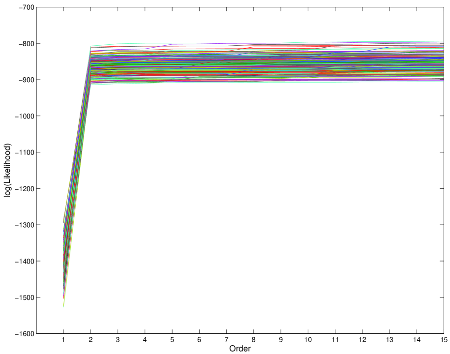
Here, we provide both a visual and numerical method to select the order. Similar to the scree plot widely used in multivariate analysis (Rencher,, 2002), we can plot against the order . When the observed series follows an AR or TVAR model, the values of will stop increasing after a specific lag, this lag can be chosen as the order for the estimated model. Henceforth, this plot is referred to as “BLF-scree.” This type of visual order determination can be directly quantified through the relative change of . Specifically, we provide a numerical method of order selection based on calculating the percent change in going from to with respect to ,
| (15) |
Based on simulation of various TVAR models, we choose with reflecting the “best” value for the order. That is, we have found that provides an effective cut-off for choosing the order. Although this approach provides a good guide to order selection, other model selection methods could be considered (e.g., shrinkage through Bayesian variable selection, reversible jump MCMC, or by minimizing an information criteria). Development of alternative model selection approaches in this setting constitutes an area of future research.
We now summarize our approach for fitting TVAR models. Given a set of hyperparameters , the procedure starts by setting , for . Next, plugging and into (5) and (6) and using sequential filtering and smoothing algorithms, we obtain a series of estimated parameters , , , and , as well as the new series of forward and backward prediction errors, and , for . We then repeat the above procedure until , , , and have been obtained. Then, recursively plugging the estimates of and , from into (7) and (8), we obtain the estimated time-varying coefficients of (1). As part of this algorithm, the series of estimated innovation variances are equal to . Finally, for , the time-frequency representation associated with the TVAR() model can be obtained by the following equation
| (16) |
where (Kitagawa and Gersch,, 1996). Plugging the estimated values , , and into (16) yields the estimated time-varying AR() time-frequency representation . See the Appendix for further discussion.
3 Simulation Studies
In this section, we simulate various nonstationary time series in order to compare the performance of our approach with four other approaches used to estimate the time-frequency representation. The first approach is AdaptSPEC proposed by Rosen et al., (2012). This approach adaptively segments the signal into finite pieces and then estimates the time-frequency representation using smoothing splines to fit local spectra via the Whittle likelihood approximation. The size of a segment and the number of the spline basis functions are two essential parameters for this approach. To reduce any subjectivity in our comparisons, we choose settings for these two parameters similar to those considered in Rosen et al., (2012) (with their ), as well as the same settings for MCMC iterations and burn-in. However, rather than using 10 spline basis functions we use 15, as this provides slightly better results along with superior computational stability. We note that the approach of Everitt et al., (2013) is not considered here due to the fact that the parameterization of the spectral density through the Wittle likelihood requires subjective knowledge.
The second approach is the AutoPARM method (Davis et al.,, 2006). Although this approach combines the GA and MDL to automatically search for potential break points along with the AR orders for each segment, four parameters are crucial for the GA: the number of islands, the number of chromosomes in each island, the number of generations for migration, and the number of chromosomes replaced in a migration; see Davis et al., (2006) for a comprehensive discussion. All of these parameters were chosen identical to those used in Davis et al., (2006).
The third approach is the AutoSLEX method (Ombao et al.,, 2001). Given a fixed value for the complexity penalty parameter of the cost function, AutoSLEX can automatically segment a given signal and choose a smoothing parameter. Following the suggestion of Ombao et al., (2001), we set this parameter equal to one. The last method we consider is the approach of West et al., (1999), referred to as WPK1999. This approach requires specification of three parameters: the TVAR order and two discount factors – one associated with the variance of the time-varying coefficients and the other with the innovation variances. In general, the discount factor values are in the range (West et al.,, 1999). Therefore, for our simulations, we give each discount factor a set of values from to (with equal spacing of ) and, further, a set of values for the TVAR order from to . Given these values, we choose the combination that achieves the maximum likelihood (West et al.,, 1999).
Our approach uses the two selection methods discussed in Section 2.5 to search for the TVAR order with appropriate discount factor values. The selected combination of with and held fixed over all stages of the Bayesian lattice filter is referred to as BLFFix. The selected combination of (), for , is referred to as BLFDyn. Again, the candidate space of parameters for both discount factors are from to (with equal spacing of ), along with orders from to .
We consider four types of nonstationary signals: 1) TVAR of order with constant innovation variance; 2) TVAR of order with constant innovation variance; 3) a piecewise AR process with constant innovation variance; and 4) simulated signals based on an Enchenopa treehopper communication signal (Holan et al.,, 2010); see Section 4.1. Each simulation consists of realizations. To evaluate the performance in estimating the various time-frequency representations, we calculate the average squared error (ASE) for each realization as follows (Ombao et al.,, 2001)
| (17) |
where , , and denotes the length of the simulated series. Lastly, we denote . For each simulation study, Table 1 summarizes the mean values and standard deviations for .
In the case of the AutoSLEX method the number of frequencies in (17) differs from the other approaches considered. In particular, the AutoSLEX approach dyadically segments the signal up to a given maximum scale such that is less than signal length, . Subsequently, AutoSLEX automatically determines whether a segment at a particular scale will be included in final segmentation. Once this has been completed, the frequency resolution for the AutoSLEX approach is equal to where is the scale of the largest segment included in the final segmentation.
3.1 Time-Varying AR(2) Process
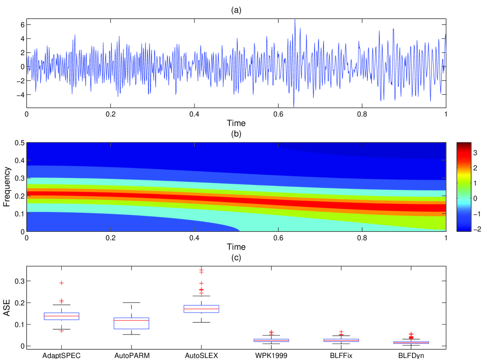
We simulate signals from the same time-varying AR(2) process (TVAR2), used in Davis et al., (2006) and Rosen et al., (2009, 2012), which is defined as follows
where and . Figure 1 shows the BLF-scree plot, suggesting that order two is the appropriate choice for all 200 realizations. Since the time-varying coefficient , varies slowly with time, this process naturally exhibits a slowly evolving time-varying spectrum (Figure 2). The box-plots of the ASE values in Figure 2 show that the group of TVAR-based models (i.e., WPK1999, BLFFix, and BLFDyn) perform superior to the group of non-TVAR-based models (i.e., AdaptSPEC, AutoPARM, and AutoSLEX), with BLFDyn performing the best. In particular, there is a significant percent reduction in for BLFDyn relative to the other methods considered (Table 1).
3.2 Time-Varying AR(6) Process
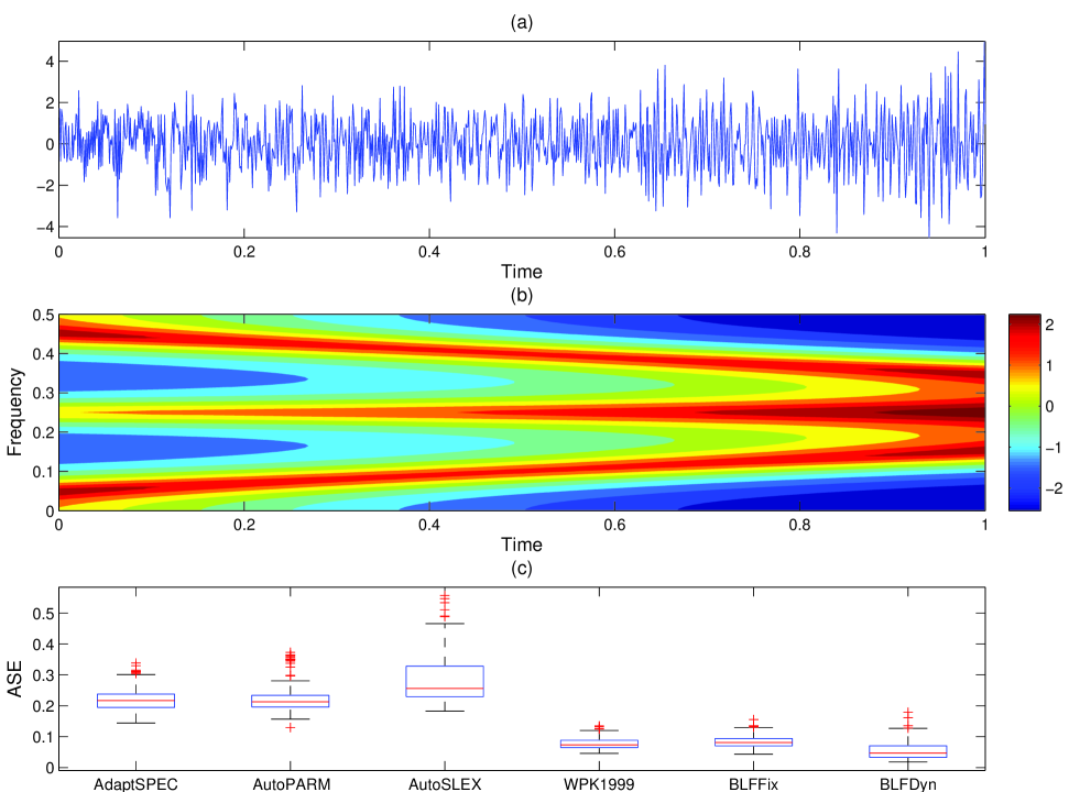
We consider signals from the same time-varying AR(6) process of order six (TVAR6) used in Rosen et al., (2009). This time-varying AR(6) process can be compactly expressed as , , in terms of a characteristic polynomial function , with and the backshift operator (i.e., ). The characteristic polynomial function for this process can be factorized as
where the superscript denotes the complex conjugate. Also, for , let , where the s are defined by
with and the values of , , and equal to , , and , respectively.
The BLF-scree plot (not shown) suggests that order six is the appropriate choice for all 200 realizations. The TVAR(6) contains three pairs of time-varying conjugate complex roots. Figure 3 illustrates that the TVAR(6) has a time-varying spectrum with three peaks. Similar to the TVAR(2) analysis (Section 3.1), the TVAR-based models outperform the group of non-TVAR-based models, with BLFDyn performing superior to the others. Again, the percent reduction in is significant relative to the other approaches considered (Table 1).
3.3 Piecewise Stationary AR Process
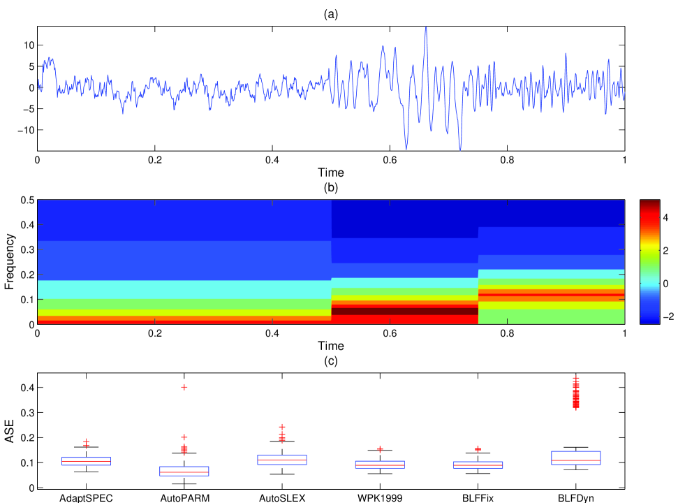
The signals simulated here are based on the same piecewise stationary AR process, used by Davis et al., (2006) and Rosen et al., (2009, 2012) and is defined as follows
where . These generated signals are referred to as PieceAR. Since it is difficult to choose the order for some realizations visually using the BLF-scree plot, we use (15), with , to choose the order. The numerical method suggests order two for some realizations and order three for the others. The true process includes three segments, with each of the segments mutually independent. The piecewise nature of this process is clearly depicted by its time-varying spectrum (Figure 4b). The box-plot (Figure 4c) shows that AutoPARM exhibits superior performance in terms of the smallest median ASE. However, WPK1999 and BLFFix may perform more robustly (i.e., less outlying ASE values). Although we see a 23.78% reduction in for AutoPARM versus BLFFix, we find that BLFFix performs superior to the remainder of the approaches and has the smallest standard deviation across the 200 simulations. Table 1 summarizes the mean values and standard deviations for this simulation. The findings here are not surprising as AutoPARM is ideally suited toward identifying and estimating piecewise AR processes. For our approach, taking fixed is advantageous for processes that are not slowly-varying.
3.4 Simulated Insect Communication Signals
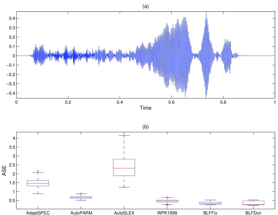
The signals considered in this simulation are formulated such that they exhibit the same properties as an Enchenopa treehopper mating signal; see Section 4.1 for a complete discussion. Specifically, we fit a TVAR(6) model to the signal , , to obtain time-varying AR coefficients and innovation variances. Typically, with these type of nonstationary signals, the innovation variances are time dependent, which is markedly different from the previous examples where the innovation variance was constant. The signals generated by these parameters are referred to as SimBugs. As expected, the BLF-scree plot (not shown) suggests that order six may be an appropriate choice for all 200 realizations. Figure 5a illustrates one realization of the SimBugs, whereas Figure 5b provides box-plots that characterize the distribution of over the 200 simulated signals. Specifically, from Figure 5b, we see that BLFFix and BLFDyn perform better than the other approaches, in terms of median ASE. Further, we find that BLFFix and BLFDyn are similar, in terms of , although the median of BLFDyn (0.2675) is smaller than that of BLFFix (0.3176).
Table 1 summarizes the mean values and standard deviations for this simulation. From this table we see that the reduction in for BLFDyn is 6.01% over BLFFix and that both exhibit a substantial percent reduction in over the other methods considered.
4 Case Studies
4.1 Animal Communication Signals
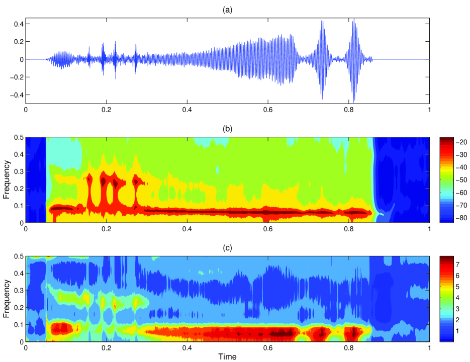
Understanding the dynamics of populations is an important component of evolutionary biology. Many organisms exhibit complex characteristics that intricately relate to fitness. For example, the mating signal of the Enchenopa treehopper represents a phenotype of the insect that is used in mate selection. During the mating season, males in competition deliver their vibrational signals through stems of plants to females (see Cocroft and McNett,, 2006, and the references therein). The data considered here comes from an experiment that was previously analyzed in Cocroft and McNett, (2006) and Holan et al., (2010). The experiment was designed with the goal of reducing potential confounding effects between environmental and phenotypical variation. In this experiment, males signals were recorded one week prior to the start of mating. Figure 6a displays a typical signal of from a successful mater, with length 4,739 downsampled from registered signals of length 37,912. Justification for the appropriateness of downsampling the original signal, in this context, can be found in Holan et al., (2010). Also, as discussed in Holan et al., (2010), this signal shows a series of broadband clicks preceding a frequency-modulated sinusoidal component, followed by a series of pulses.
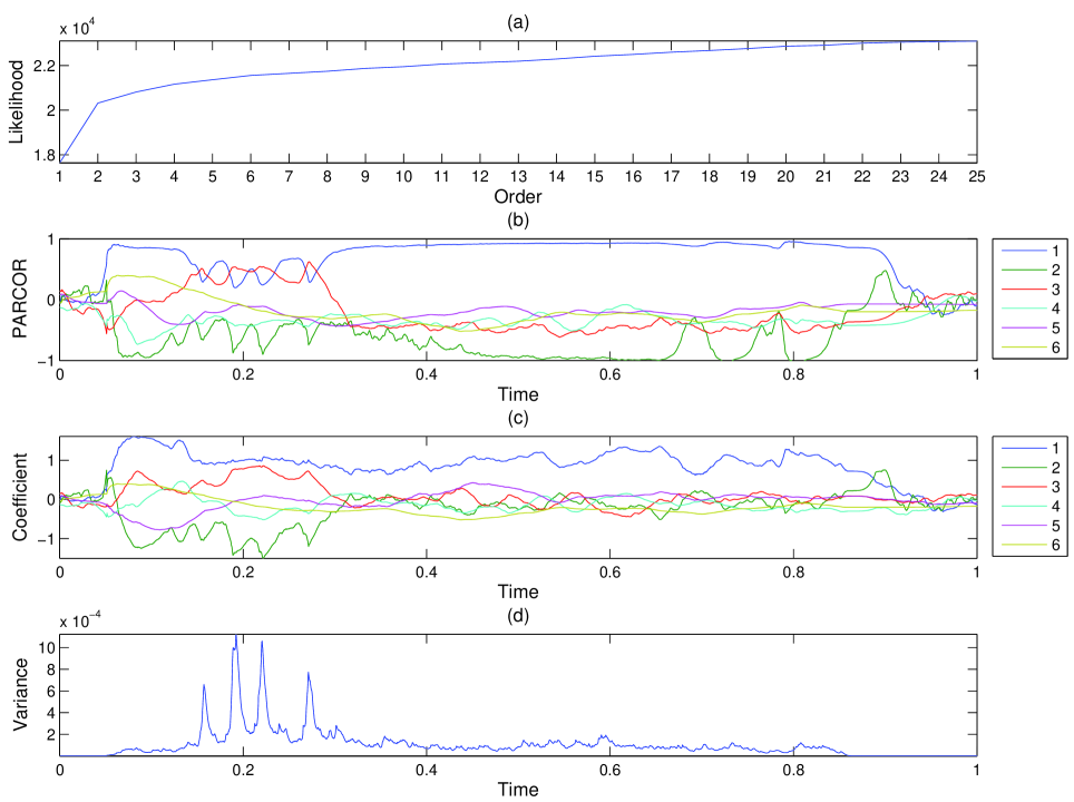
For this analysis, we used the BLFDyn approach to search for a model having both discount factors in the range of to (with equal spacing of ) and an order between and . Figure 7a shows an increase in along with the order, which is different from the simulated TVAR(6) model in Section 3.4. Hence, we use (15) with the model order chosen by . This rule yields a TVAR(6) model. In Figure 7b, the PARCOR coefficients of lag larger than two are close to zero following time around (where the time axis has been normalized such that ). Thus, the last four TVAR coefficients after time are close to zero (Figure 7c). Such phenomena suggests that the period before time has a more complex dependence structure. Figure 7d illustrates that the innovation variance exhibits higher volatility at the beginning signal. These bursts in the innovation variance are related to the series of broadband clicks at the beginning of the signal. Finally, Figure 6b presents the time-frequency representation of the treehopper signal using the TVAR(6) model and corroborates the significance of the broadband clicks at the beginning of the signal. Figure 6c shows the posterior standard deviation of the time-frequency representation using 2,000 MCMC samples from 210,000 MCMC iterations by discarding the first 10,000 iterations as burn-in and keeping every 100-th iteration of the remainder.
4.2 Wind Components
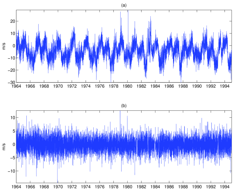
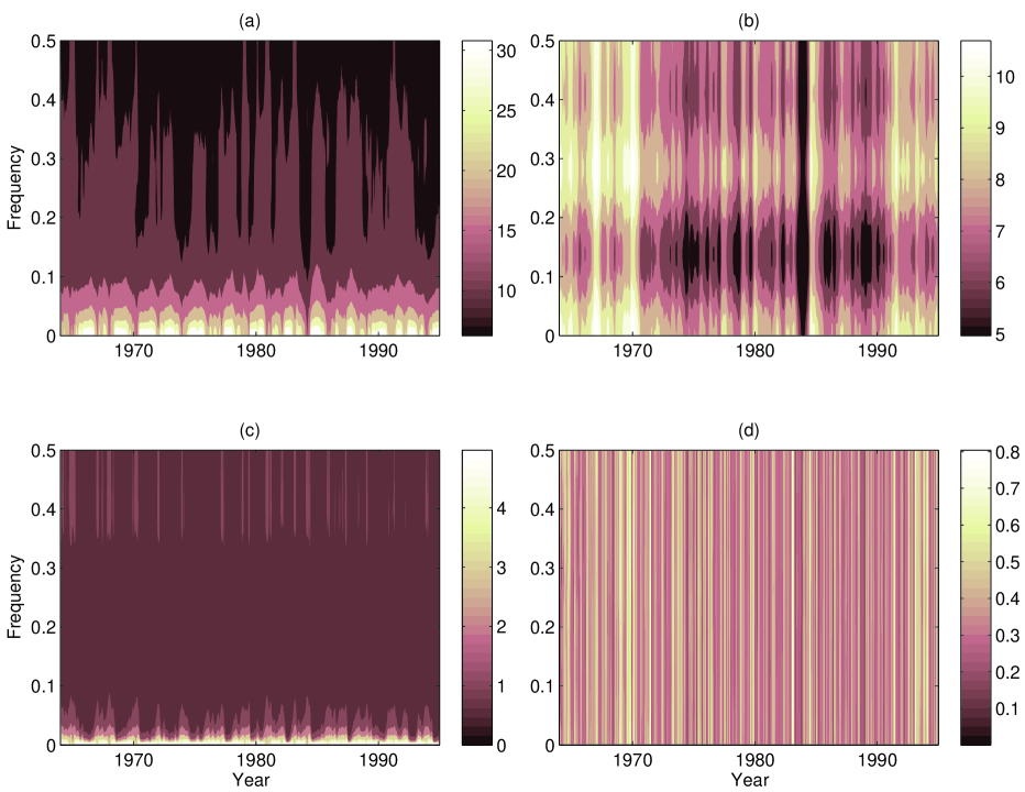
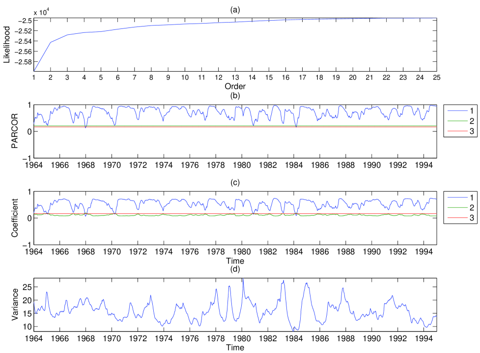
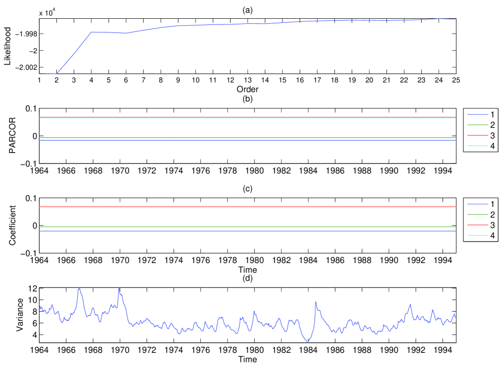
We study the time-frequency representations of the east/west and north/south wind components, recorded daily at Chuuk Island in the tropical Pacific during the period of 1964 to 1994 (see Cressie and Wikle,, 2011, Sections 3.5.3 and 3.5.4). The data studied are at the level of 70 hPa, which is important scientifically due to the likely presence of westward and eastward propagating tropical waves, and the presence of the quasi-biennial oscillation (QBO) (Wikle et al.,, 1997). Figure 8 shows the two wind component time series from which we can discern visually that the east/west series clearly exhibits the QBO signal, but no discernible smaller-scale oscillations are present in either series. Our interest is then whether the time-varying spectra for these series suggest the presence of time-varying oscillations, which are theorized to be present.
We consider the same search space for the model order and discount factors as that used for the treehopper communication signal (Section 4.1). The BLF-scree plot for the east/west component shows an increase of along with the order. Therefore, we use (15) with and choose the order equal to three. The PARCOR coefficient of lag one depends on time but the PARCOR coefficient of lag two and three appear to be constant. The innovation variances of TVAR(3) model are time dependent. On the other hand, the BLF-scree plot for the north/south component shows a turning point at order four so that we choose the order equal to four. The PARCOR coefficients are time independent but the innovation variances of the TVAR(4) model are time dependent. The preceding findings are illustrated in Figures 13 and 14 of the Appendix. Figures 9a and 9b show the estimated time-frequency representations of the wind east/west and north/south components. Figures 9c and 9d present the associated posterior standard deviations of the time-frequency representation using 2,000 MCMC samplers from 210,000 MCMC iterations by discarding the first 10,000 iterations as burn-in and keeping every 100-th iteration of the remainder. The east/west component time-varying spectrum does suggest that the QBO intensity varies considerably as evidenced by the power in the low-frequencies. Perhaps more interesting is the suggestion of time-varying equatorial waves in the north/south wind component time-varying spectrum. In particular, the lower-frequency (Kelvin and Rossby) waves with frequencies between 0.1 and 0.2 show considerable variation in duration of wave activity, as well as intensity. One also sees time-variation in the likely mixed-Rossby gravity waves in the frequency band between 0.2 and 0.35. Interestingly, in some cases these are in phase with the lower-frequency wave activity but more often act in opposition. We also note the almost complete collapse of the equatorial wave activity centered on 1984.
4.3 Economic Index
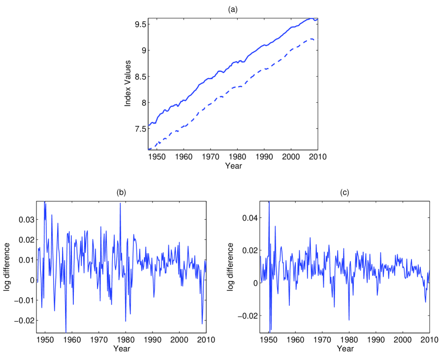
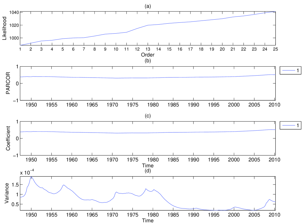
Koopman and Wong, (2011) study the time-frequency representation of the log difference of the US gross domestic product (GDP), consumption, and investment from the first quarter of 1947 to the first quarter of 2010. For comparison, we obtained the series from the Federal Reserve Bank of St. Louis http://research.stlouisfed.org/fred2. Since the investment series is unavailable from the website, we only consider the GDP and consumption in our study. Figure 10a illustrates the trend of the logarithm of the GDP and consumption series. Similar to Koopman and Wong, (2011), we analyzed the log difference of these two series (Figures 10b and 10c).
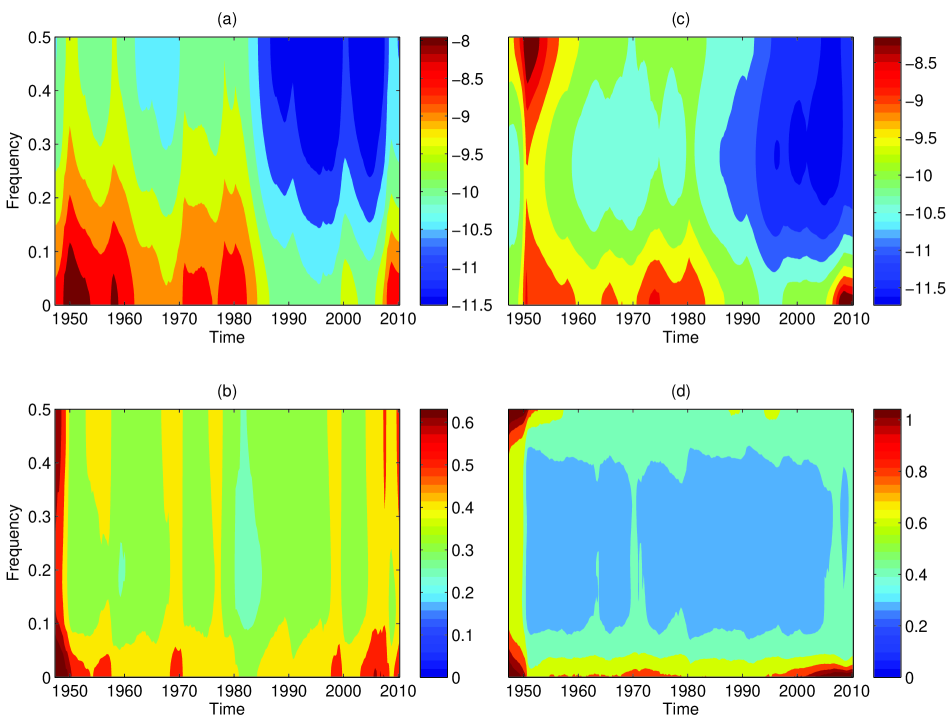
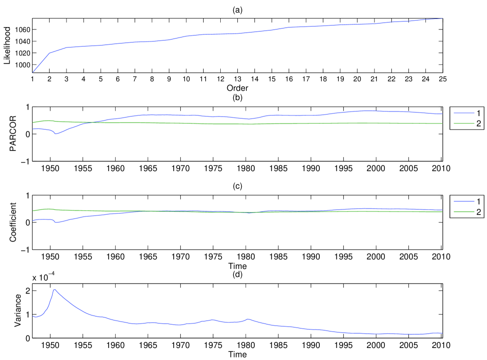
We consider the same search space for the model order and discount factors as that used for the treehopper communication signal (Section 4.1). By using (15) with , we choose TVAR(1) for the log difference of GDP and TVAR(2) for the log difference of consumption. Figures 11a and 11b show the estimated time-frequency representations and the associated standard deviations of the log difference of GDP and consumption series, respectively. Similar to the results of Koopman and Wong, (2011), both the US macroeconomic indices exhibit relatively larger spectra (or fluctuations) for the early period around 1950. Then, due to the oil crisis, another fluctuation comes out in the period of 1970–1980. The fluctuation at the end of the sample reflects the 2008–2009 worldwide financial crisis. See Koopman and Wong, (2011) for further discussion. Using the same MCMC iterations as Section 4.1, Figures 11c and 11d present the associated posterior standard deviations.
5 Discussion
This paper develops a computationally efficient method for model-based time-frequency analysis. Specifically, we consider a fully Bayesian lattice filter approach to estimating time-varying autoregressions. By taking advantage of the partial autocorrelation domain, our approach is extremely stable. That is, the PARCOR coefficients and the TVAR innovation variances are specified within the lattice structure and then estimated simultaneously. Notably, the full conditional distributions arising from our approach are all of standard form and, thus, facilitate easy estimation.
The framework we propose extends the current model-based approaches to time-frequency analysis and, in most cases, provides superior performance, as measured by the average squared error between the true and estimated time-varying spectral density. In fact, for slowly-varying processes we have demonstrated significant estimation improvements from using our approach. In contrast, when the true process comes from a piecewise AR model the approach of Davis et al., (2006) performed best, with our approach a close competitor and performing second best. This is not unexpected as the AutoPARM method is a model-based segmented approach and more closely mimics the behavior of a piecewise AR.
In addition to a comprehensive simulation study we have provided three real-data examples, one from animal (insect) communication, one from environmental science, and one from macro-economics. In all cases, the exceptional time-frequency resolution obtained using our approach helps identify salient features in the time-frequency surface. Finally, as a by-product of taking a fully Bayesian approach, we are naturally able to quantify uncertainty and, thus, use our approach to draw inference.
Acknowledgments
This research was partially supported by the U.S. National Science Foundation (NSF) and the U.S. Census Bureau under NSF grant SES-1132031, funded through the NSF-Census Research Network (NCRN) program. The authors would like to thank the Reginald Cocroft lab for use of the insect communication data analyzed in Section 4.1. The authors would like to thank Drs. Richard Davis, Hernando C. Ombao, and Ori Rosen for providing their codes. Finally, we also thank Dr. Mike West for generously providing his code online.
| () | ||||||
|---|---|---|---|---|---|---|
| AdaptSPEC | AutoPARM | AutoSLEX | WPK1999 | BLFFix | BLFDyn | |
| TVAR2 | 0.1383 (0.0275) | 0.1085 (0.0302) | 0.1735 (0.0333) | 0.0268 (0.0093) | 0.0269 (0.0093) | 0.0170 (0.0084) |
| TVAR6 | 0.2195 (0.0351) | 0.2233 (0.0439) | 0.2885 (0.0796) | 0.0771 (0.0171) | 0.0841 (0.0191) | 0.0543 (0.0276) |
| PieceAR | 0.1070 (0.0227) | 0.0702 (0.0392) | 0.1141 (0.0296) | 0.0931 (0.0218) | 0.0921 (0.0205) | 0.1607 (0.1107) |
| SimBugs | 1.4760 (0.2237) | 0.6711 (0.0725) | 2.3993 (0.6078) | 0.4627 (0.0796) | 0.3444 (0.0659) | 0.3237 (0.1075) |
Appendix A: Sequential Updating and Smoothing
To complete the Bayesian estimation of the forward and backward PARCOR coefficients, as well as the time-varying innovation variances, we use dynamic linear models (DLMs) (see, West and Harrison,, 1997; Prado and West,, 2010). Specifically, we provide the details and formulas for analysis of and . The analysis of and follow similarly.
For , given the values of and at stage , recall (5) of Section 2.3 gives
with . Modeling of and proceeds using (9) and (11):
with (see West and Harrison,, 1997, Section 6.3) and the scale parameter of the marginal -distribution of given the information up to time . Moreover, , and (see West and Harrison,, 1997, Section 10.8), where the shape parameter of the marginal gamma distribution of given the information up to time (see Section A.1). Then, given specified values for the two discount factors and , as well as conditional on assuming conjugate initial priors (13) and (14), we can specify the corresponding sequential updating and smoothing algorithms using DLM theory.
A.1 Sequential Updating
Using similar notation to West and Harrison, (1997) and West et al., (1999), we first sequentially update the joint posterior distributions of over Since the initial priors have the conjugate normal/gamma forms, also has the normal/gamma form. Therefore, the marginal posterior distribution of is a -distribution; i.e., , with degrees of freedom , location parameter , and scale parameter . The marginal posterior distribution of is a gamma distribution , with shape parameter and scale parameter . We summarize the sequential updating equations of parameters for , as follows:
and
where
Importantly, since , we can reduce to .
A.2 Smoothing
After the sequential updating process, we can use a retrospective approach to specify the smoothing joint distribution of , for , given all the information up to time (West and Harrison,, 1997; West et al.,, 1999). We summarize the equations for the parameters of both marginal distributions, , with degrees of freedom , location parameter , and scale parameter . Moreover, , with shape parameter and scale parameter . It is important to note that when , we have , , , and from the results of sequential updating. Additionally, the point estimate of at time is . Then, for , we can summarize the equations as follows:
A.3 Algorithm for Fitting TVAR Models
We summarize the algorithm of our approach to fitting a TVAR() model as follows:
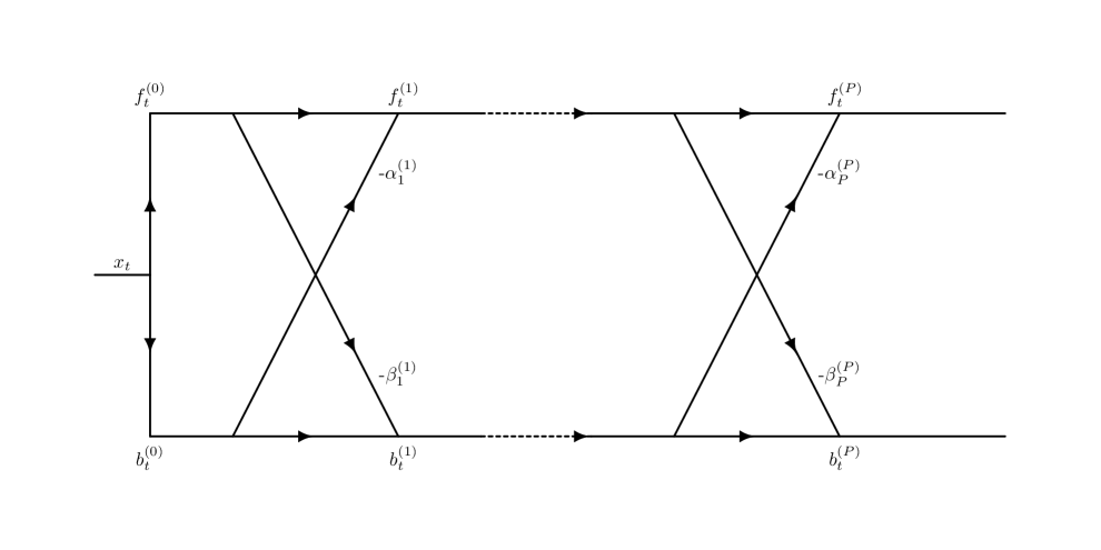
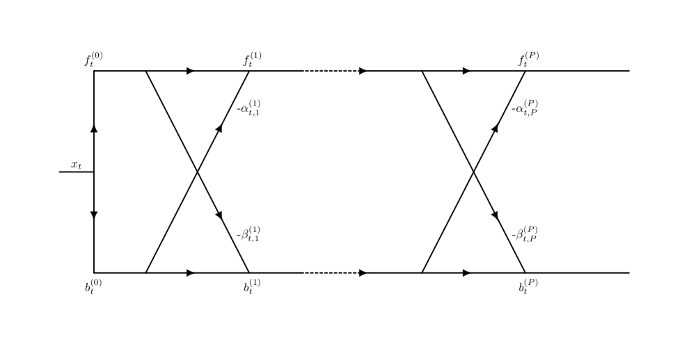
Appendix B: Lattice Filter Structure
Figure 12a illustrates the lattice structure for an AR() model. Given and , , recursive use of (2) and (3) can produce forward and backward prediction errors for the forward and backward AR() models (i.e., and ). Alternatively, Figure 12b illustrates the lattice structure for a TVAR() model. Different from Figure 12a, the forward and backward PARCOR coefficients are time dependent. Given and , , this case presents recursive use of (5) and (6) to produce forward and backward prediction errors for the forward and backward TVAR() model.
| (a) |
 |
| (b) |
 |
Appendix C: Supplemental Figures for Case Studies
This section contains supplemental figures associated with Section 4 of the main text (Case Studies). These figures are not strictly necessary to illustrate the intended applications. Nevertheless, we include them here for further potential scientific insight.
Figures 13a and 14a provide BLF-scree plots associated with the east/west and north/south components of the wind signal. The first three time-varying estimated PARCOR coefficients of the east/west and north/south components of the wind signal are provided in Figures 13b and 14b. The estimated time-varying coefficients of the TVAR(3) model for the east/west component are given in Figures 13c and 13d whereas the estimated time-varying coefficients of the TVAR(4) model for the north/south component are given in Figures 14c and 14d. Finally, the BLF-scree plot, time-varying estimated PARCOR coefficients and time-varying innovation variances for the difference of the logarithm GDP and Consumptions series are provided in Figures 15 and 16.
References
- Cocroft and McNett, (2006) Cocroft, R. B. and McNett, G. D. (2006). “Vibrational communication in treehoppers (Hemiptera: Membracidae).” In Insect Sounds and Communication: Physiology, Ecology and Evolution, S. Drosopoulos and M. F. Claridge (Eds.), 305–317. Taylor & Francis.
- Cressie and Wikle, (2011) Cressie, N. and Wikle, C. K. (2011). Statistics for Spatio-Temporal Data. John Wiley & Sons.
- Davis et al., (2006) Davis, R. A., Lee, T. C. M., and Rodriguez-Yam, G. A. (2006). “Structural break estimation for nonstationary time series models.” Journal of the American Statistical Association, 101, 473, 223–239.
- Everitt et al., (2013) Everitt, R. G., Andrieu, C., and Davy, M. (2013). “Online Bayesian inference in some time-frequency representations of non-stationary processes.” IEEE Transactions of Signal Processing, 61, 5755–5766.
- Feichtinger and Strohmer, (1998) Feichtinger, H. G. and Strohmer, T. (1998). Gabor Analysis and Algorithms: Theory and Applications. Birkhauser.
- Fitzgerald et al., (2000) Fitzgerald, W. J., Smith, R. L., Walden, A. T., and Young, P. C. (2000). Nonlinear and Nonstationary Signal Processing. Cambridge University Press.
- Godsill et al., (2004) Godsill, S. J., Doucet, A., and West, M. (2004). “Monte Carlo smoothing for nonlinear time series.” Journal of the American Statistical Association, 99, 465, 156–168.
- Gröchenig, (2001) Gröchenig, K. (2001). Foundations of Time-Frequency Analysis. Birkhauser.
- Hayes, (1996) Hayes, M. H. (1996). Statistical Digital Signal Processing and Modeling. John Wiley & Sons.
- Haykin, (2002) Haykin, S. (2002). Adaptive Filter Theory (4th ed). Pearson.
- Holan et al., (2010) Holan, S. H., Wikle, C. K., Sullivan-Beckers, L. E., and Cocroft, R. B. (2010). “Modeling complex phenotypes: generalized linear models using spectrogram predictors of animal communication signals.” Biometrics, 66, 3, 914–924.
- Holan et al., (2012) Holan, S. H., Yang, W.-H., Matteson, D. S., and Wikle, C. K. (2012). “An approach for identifying and predicting economic recessions in real-time using time-frequency functional models.” Applied Stochastic Models in Business and Industry, 28, 485–499.
- Kitagawa, (1988) Kitagawa, G. (1988). “Numerical approach to non-Gaussian smoothing and its applications.” In Proceedings of the 20th Symposium on the Interface, ed. J. M. E.J. Wegman, D.T. Gantz. Interface Foundation of North America.
- Kitagawa, (2010) — (2010). Introduction to Time Series Modeling. Chapman & Hall/CRC.
- Kitagawa and Gersch, (1996) Kitagawa, G. and Gersch, W. (1996). Smoothness Priors Analysis of Time Series. Springer.
- Koopman and Wong, (2011) Koopman, S. and Wong, S. (2011). “Kalman filtering and smoothing for model-based signal extraction that depend on time-varying spectra.” Journal of Forecasting, 30, 147–167.
- Mallat, (2008) Mallat, S. G. (2008). A Wavelet Tour of Signal Processing: The Sparse Way. Academic Press.
- Ombao et al., (2001) Ombao, H., Raz, J., Von Sachs, R., and Malow, B. (2001). “Automatic statistical analysis of bivariate nonstationary time series.” Journal of the American Statistical Association, 96, 454, 543–560.
- Oppenheim and Schafer, (2009) Oppenheim, A. V. and Schafer, R. W. (2009). Discrete-Time Signal Processing. Prentice Hall Signal Processing.
- Percival and Walden, (2000) Percival, D. B. and Walden, A. T. (2000). Wavelet Methods for Time Series Analysis. Cambridge University Press.
- Prado and Huerta, (2002) Prado, R. and Huerta, G. (2002). “Time-varying autogressions with model order uncertainty.” Journal of Time Series, 23, 5, 599–618.
- Prado and West, (2010) Prado, R. and West, M. (2010). Time series: modeling, computation, and inference. CRC Press.
- Rencher, (2002) Rencher, A. C. (2002). Methods of Multivariate Analysis (2nd ed). John Wiley & Sons.
- Rosen et al., (2009) Rosen, O., Stoffer, D. S., and Wood, S. (2009). “Local spectral analysis via a Bayesian mixture of smoothing splines.” Journal of the American Statistical Association, 104, 485, 249–262.
- Rosen et al., (2012) Rosen, O., Wood, S., and Stoffer, D. S. (2012). “AdaptSPEC: Adaptive spectral estimation for nonstationary time series.” Journal of the American Statistical Association, 107, 500, 1575–1589.
- Shumway and Stoffer, (2006) Shumway, R. H. and Stoffer, D. S. (2006). Time Series Analysis and Its Applications (2nd ed). Springer.
- Vidakovic, (1999) Vidakovic, B. (1999). Statistical Modeling by Wavelets. John Wiley & Sons.
- West and Harrison, (1997) West, M. and Harrison, J. (1997). Bayesian Forecasting and Dynamic Models (2nd ed). Springer.
- West et al., (1999) West, M., Prado, R., and Krystal, A. D. (1999). “Evaluation and comparison of EEG traces: latent structure in nonstationary time series.” Journal of the American Statistical Association, 94, 446, 375–387.
- Wikle et al., (1997) Wikle, C. K., Madden, R. A., and Chen, T.-C. (1997). “Seasonal variation of upper tropospheric lower stratospheric equatorial waves over the tropical Pacific.” Journal of the Atmospheric Sciences, 54, 1895–1909.
- Wolfe et al., (2004) Wolfe, P. J., Godsill, S. J., and Ng, W. J. (2004). “Bayesian variable selection and regularization for time–frequency surface estimation.” Journal of the Royal Statistical Society: Series B (Statistical Methodology), 66, 3, 575–589.
- Wood et al., (2011) Wood, S., Rosen, O., and Kohn, R. (2011). “Bayesian mixtures of autoregressive models.” Journal of Computational and Graphical Statistics, 20, 1, 174–195.
- Yang et al., (2013) Yang, W.-H., Wikle, C. K., Holan, S. H., and Wildhaber, M. L. (2013). “Ecological prediction with nonlinear multivariate time-frequency functional data models.” Journal of Agricultural, Biological, and Environmental Statistics, 18, 3, 450–474.